Adsorption of solutes at liquid-vapor interfaces: Insights from lattice gas models

Abstract

The adsorption behavior of ions at liquid-vapor interfaces exhibits several unexpected yet generic features. In particular, energy and entropy are both minimum when the solute resides near the surface, for a variety of ions in a range of polar solvents, contrary to predictions of classical theories. Motivated by this generality, and by the simple physical ingredients implicated by computational studies, we have examined interfacial solvation in highly schematic models, which resolve only coarse fluctuations in solvent density and cohesive energy. Here we show that even such lattice gas models recapitulate surprising thermodynamic trends observed in detailed simulations and experiments. Attention is focused on the case of two dimensions, for which approximate energy and entropy profiles can be calculated analytically. Simulations and theoretical analysis of the lattice gas highlight the role of capillary wave-like fluctuations in mediating adsorption. They further point to ranges of temperature and solute-solvent interaction strength where surface propensity is expected to be strongest.

I Introduction

Experiments and computer simulations have demonstrated that certain small ions preferentially adsorb at liquid-vapor interfaces Jungwirth and Tobias (2006, 2002); Petersen and Saykally (2004); Noah-Vanhoucke and Geissler (2009); Otten et al. (2012), contrary to expectations from classic theories of ion solvation Onsager and Samaras (1934). Efforts to explain this behavior have focused primarily on accounting for effects of solute polarizability and the thermodynamic cost of excluding volume in bulk solution Jungwirth and Tobias (2006); Archontis and Leontidis (2006); Levin (2009); Levin et al. (2009); Markin and Volkov (2002). For small excluded volumes, this cost is primarily entropic and reflects constraints on the available arrangements of nearby solvent molecules. Huang and Chandler (2002). From this perspective the adsorption of a non-polarizable ion is expected to be opposed energetically (through loss of dielectric polarization energy) and favored entropically (through recovered freedom of local solvent arrangements). Very recent work has shown, however, that these thermodynamic driving forces generally follow the opposite trend, with energy and entropy both exhibiting minima when an ion resides near the interface Otten et al. (2012); Caleman et al. (2011); Iuchi et al. (2009). In these studies we and others also revealed important driving forces governing ion adsorption that had been largely ignored in discussions of interfacial solvation.

The interface between a dense polar liquid and its coexisting vapor is a region of high energy density (relative to that of the bulk liquid), due to incomplete or strained coordination of solvent molecules. The liquid’s boundary can nonetheless be quite soft, with substantial wavelike shape fluctuations even on molecular length scales. These generic facts appear from simulations to have important consequences for the thermodynamics of ion adsorption. In particular, moving a solute from bulk solution to the interface effects more than reduced coordination of the ion (which is exclusively emphasized in classic theories). An adsorbed solute also occupies volume in the high-energy region, effectively returning solvent density to the bulk environment Stuart and Berne (1996); Vaitheeswaran and Thirumalai (2006); Otten et al. (2012). The consequence of this simple but often overlooked accounting is a substantially favorable energetic contribution. For ions of modest size it is sufficient to render adsorption energies negative Stuart and Berne (1996); Vaitheeswaran and Thirumalai (2006); Otten et al. (2012); Caleman et al. (2011); Iuchi et al. (2009). Although electrostatic forces clearly figure prominently in this mechanism, their long spatial range is not manifested by the dominant energetic changes accompanying adsorption Otten et al. (2012). Instead, a spatially local approximation, which expresses the total energy in terms of the populations of different solvent regions (bulk, interface, and solute coordination zone),

$$U_{local}=\epsilon_{bulk}n_{bulk}+\epsilon_{interface}n_{interface}+\epsilon_{coord}n_{coord}\,,$$ (1)

was found to be quite accurate for systems with non-polarizable ions Otten et al. (2012). Here, $\epsilon_{\gamma}$ is the energy per molecule of solvent in region $\gamma$, and $n_{\gamma}$ is the corresponding number of molecules in that region.

Softness of the interface, also neglected by conventional theories, is implicated by these simulations to significantly influence the entropy of adsorption Otten et al. (2012). A solute that substantially attracts solvent, such as an ion in water, tends to suppress surface undulations when it resides near the interface. The entropic cost of this suppression can be considerable, opposing adsorption by many $k_{\rm B}T$. Harmonic analysis of capillary wave-like fluctuations in the adsorbed and non-adsorbed states was found to roughly account for observed entropy profiles Otten et al. (2012).

The two physical ingredients speculated in Ref. Otten et al. (2012) to be key for ion adsorption, namely surface shape fluctuations and heterogeneous energy density near the liquid’s boundary, are so generic as to be described by the very simplest microscopic models of the liquid state. Motivated by this apparent generality, we examine in this paper the classic reduced model of liquid-vapor coexistence, suitably adapted to address questions of solvation. Specifically, we consider a two-dimensional lattice gas, with a solute that occupies a single lattice cell and attracts only its nearest neighbors. Presenting results of both theory and simulation, we demonstrate that the unexpected thermodynamic trends revealed by recent atomistic simulations can indeed be captured by such a simple model. The very limited microscopic detail in the case of a lattice gas allows unambiguous conclusions regarding the source of energy and entropy changes as the solute moves through the interface. It allows as well crude predictions for the varying propensity ions exhibit for liquid-vapor interfaces.

The rest of the paper is organized as follows. In Sec. II, we describe our lattice gas model for solvation. We present results of Monte Carlo simulations in Sec. III. In Sec. IV we develop a theory for the behavior of this model based on the so-called solid-on-solid simplification and compare its predictions with numerical results. We conclude in Sec. V with a discussion of specific implications for three-dimensional molecular systems.

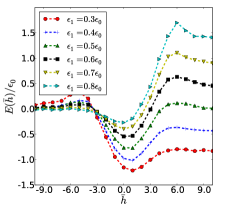
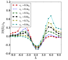
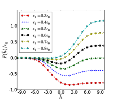
Figure 1: Profiles of (a) energy $E(\bar{h})$, (b) entropy $S(\bar{h})$, and (c) free energy $F(\bar{h})$, as a function of the height of the solute, $\bar{h}$, for various values of $\epsilon_{1}$ at $T=\epsilon_{0}/3k_{B}$. The height of $\bar{h}=0$ coincides with the GDS. These profiles were obtained from Monte Carlo simulations of the lattice gas.

II Lattice gas model

We consider a two-dimensional $L\times L$ lattice gas system with a single solute, that occupies one lattice cell. Cells are indexed by a horizontal coordinate $x$ ranging from 1 to $L$ and a vertical coordinate $y$ ranging from $-(L-1)/2$ to $(L-1)/2$ . The x-coordinate of the solute is constrained to $x=(L+1)/2$. The solute interacts only with the 4 nearest neighbor cells. It additionally excludes volume, so that a cell may not be simultaneously occupied by both solvent and solute. This system is described by the Hamiltonian

$$H=H_{0}-\epsilon_{1}\sum_{i,j\in nn}n^{s}_{i}n_{j},$$ (2)

where

$$H_{0}\equiv-{\epsilon_{0}}\sum_{i,j\in nn}n_{i}n_{j}-\mu\sum_{i}n_{i}$$ (3)

describes the pure solvent. The occupation variables $n$ and $n_{i}^{s}$ are binary: $n_{i}=1$ if the $i^{th}$ lattice site is occupied by a solvent and zero otherwise, $n^{s}_{i}=1$ if the $i^{th}$ lattice site is occupied by a solute and zero otherwise. $\sum_{i,j\in nn}$ denotes a sum over all nearest neighbor lattice pairs $i$, $j$. The coupling constant $\epsilon_{0}>0$ describes attraction between neighboring solvent cells; $\epsilon_{1}$ is the solvent-solute coupling constant.

For both theory and simulation we work with a grand canonical ensemble, in which the number of solvent cells can fluctuate subject to chemical potential $\mu$. (The number of solute cells is fixed.) Conditions of liquid-vapor coexistence are imposed by setting $\mu=-2\epsilon_{0}$, and applying boundary conditions that favor liquid in $y<0$ and vapor in $y>0$. Specifically, lattice cells with $y=-(L-1)/2$ are constrained to be occupied by solvent; those with $y=(L-1)/2$ are constrained to be unoccupied (i.e., vapor).

The mean interface position, or the Gibbs Dividing Surface (GDS), is fixed at $y=0$ by constraining as well the state of lattice cells with $x=1$ and $x=L$; those with $y<0$ are occupied, and those with $y>0$ are unoccupied.

We will examine values of $\epsilon_{1}$ between 0 and 1. By symmetry (see Appendix A), a solute with $\epsilon_{1}=\epsilon_{0}/2$ is equally likely to reside in a cell well within the liquid phase as in a cell well within the vapor phase. Judging by the free energy of transfer from liquid to vapor, one would therefore consider solutes with $\epsilon_{1}<\epsilon_{0}/2$ to be solvophobic, and those with $\epsilon_{1}>\epsilon_{0}/2$ to be solvophilic (although the latter may attract solvent significantly less strongly than adjacent solvent cells attract each other).

Using theory and simulation, we have determined the free energy $F$, average energy $E$, and the entropy $S$ as functions of the height $\bar{h}$ of the solute (i.e., its $y$-coordinate).

III Monte Carlo Simulations

We present results of Monte Carlo simulations at temperature $T=\epsilon_{0}/3k_{\rm B}$ (well below the critical temperature $T_{c}\approx\epsilon_{0}/1.764k_{\rm B}$) for a lattice with linear dimension $L=30$. Trial moves included (i) changing the state of a cell from solvent to vapor, (ii) changing a cell from vapor to solvent, and (iii) translating the solute along the $y$ axis from a lattice cell $s$ to a cell $s^{\prime}$. In the case of solute displacements, two different trial moves were used, distinguished by their treatment of solvent occupation in the cell $s$ vacated by the solute. In one move, cell $s$ adopts the previous state of $s^{\prime}$, i.e., $n_{s}^{trial}=n_{s^{\prime}}$. In another move, cell $s$ adopts the complementary state of $s^{\prime}$, i.e., $n_{s}^{trial}=1-n_{s^{\prime}}$. In all cases detailed balance was ensured through appropriate Metropolis acceptance criteria, preserving the Boltzmann distribution $p(\{n_{i},n_{i}^{s}\})\propto e^{-\beta H}$, where $\beta=1/k_{\rm B}T$ is inverse temperature.

We obtained estimates of $F(\bar{h})$ by computing the equilibrium probability $p(\bar{h})\propto\exp[-\beta F(\bar{h})]$ that the solute resides at height $\bar{h}$. The average energy $E(\bar{h})$ was estimated directly from simulations, while estimates of the entropy $S(\bar{h})$ were calculated from $TS(\bar{h})=E(\bar{h})-F(\bar{h})$.

The profiles of $F(\bar{h})$, $E(\bar{h})$, and $S(\bar{h})$ obtained from simulations with $\epsilon_{1}/\epsilon_{0}=\{0.3,0.4,0.5,0.6,0.7,0.8\}$, are plotted in Figs. 1. These results echo several nontrivial thermodynamic trends observed in molecular simulations. In particular, free energy profiles for $\epsilon_{1}=\{0.4\epsilon_{0},0.5\epsilon_{0},0.6\epsilon_{0},0.7\epsilon_{0}\}$ exhibit minima near $\bar{h}=0$. These solutes adsorb to the interface, i.e., their density at $\bar{h}=0$ is higher than in either bulk phase. Entropy minima at the same values of $\epsilon_{1}$ indicate that this adsorption reduces the diversity of accessible solvent configurations. The driving force for surface propensity is instead energetic, as evidenced by strong minima in $E(\bar{h})$ near $\bar{h}=0$. Interestingly, adsorption is strongest for the case $\epsilon_{1}=\epsilon_{0}/2$, at the crossover between solvophobic and solvophilic regimes.

These trends were also observed in simulations with smaller and larger system sizes ($L=\{20,30,40,50,60,70\}$), and for various temperatures in the range $\epsilon_{0}/5k_{B}\leq T\leq\epsilon_{0}/2k_{B}$. In all cases, profiles of free energy, energy, and entropy exhibit minima when the solute is at the interface, and maximum adsorption occurs at $\epsilon_{1}=\epsilon_{0}/2$.

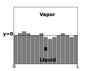
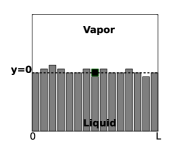
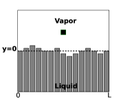
Figure 2: Illustration of three configurational subensembles in the RSOS model. The fully solvated in state (a) features a liquid vapor interface entirely above the solute. In the pinned state subensemble (b), this interface directly contacts the solute. In the unsolvated state out state, (c), the interface lies below the solute.

IV Theory

The 2-d lattice gas model of solvation described by Eq. 2, within approximations that are well justified for $T\ll T_{c}$, is sufficiently simple to permit an analytical solution. This section presents our mathematical analysis, which draws heavily on results from theoretical studies of surface roughening in Ising-like models. Weeks (1977); Chui and Weeks (1981); Abraham (1980); Fisher (1984) Our key assumptions are that the liquid-vapor interface is well defined and that the solute does not significantly alter fluctuations within either phase. More specifically, we restrict attention to the so-called “solid-on-solid” (SOS) limit Nelson et al. (2004); Temperley (1952), in which: (1) all cells in the liquid phase are occupied by solvent (except the cell occupied by the solute when it is present), (2) all cells in the vapor phase are unoccupied (except the solute cell), and (3) the boundary between liquid and vapor is a single-valued function of $x$. With this neglect of bubbles, islands, and overhangs, a configuration can be specified through the heights of $L$ columns representing the instantaneous domain of the liquid phase.

Under conditions of coexistence, the Hamiltonian describing the solvent is then given by Nelson et al. (2004); Safran (2003)

$$\bar{H_{0}}=\frac{\epsilon_{0}}{2}\sum_{i,j\in nn}|h_{i}-h_{j}|\,,$$ (4)

where $h_{i}$ denotes the height of the liquid in the $i^{th}$ column. Boundary conditions described in Sec. II fix the heights of the first and last columns, $h_{1}=0$ and $h_{L}=0$. They also bound the range of column height fluctuations, $-L/2<h_{i}<L/2$. As an added simplification, we work with the Restricted SOS (RSOS) model Chui and Weeks (1981) where the height difference between neighboring columns is constrained to be at most 1, $|h_{i}-h_{i+1}|\leq 1$. A few allowed configurations of the RSOS model are illustrated in Fig 2. Previous work has shown that fluctuations of the neat liquid-vapor interface of a two-dimensional lattice gas are well described by the RSOS model for temperatures $T\ll T_{c}$ Chui and Weeks (1981); Fisher (1984). As in that work, the restriction on height fluctuations is necessary to derive simple closed form expressions for thermodynamic quantities of interest.

The liquid-vapor interface of the RSOS model supports shape fluctuations akin to capillary waves. It has been shown in particular that long-wavelength Fourier modes are Gaussian distributed to a good approximation. For a 2-d RSOS interface of length $M$, whose boundaries are fixed at $h_{1}=p$ and $h_{M}=q$, the partition function is given by  Chui and Weeks (1981); Fisher (1984); Kardar (2007)

$$Z^{1,M}(p,q)\approx\frac{e^{2aM}}{\sqrt{4\pi aM}}\exp\left[{\frac{-(p-q)^{2}}{4aM}}\right]\,,$$ (5)

in the limit $Ma>>1$, where $a\equiv\exp(-\beta\epsilon_{0}/2)$. This result is strictly valid only in the low temperature limit, where terms of order $O(a^{2})$ can be neglected. Empirically, however, the thermodynamic properties we compute using Eq. 5 agree well with those obtained from lattice gas simulations even at moderate temperatures.

To construct a theory for interfacial solvation from Eq. 5, we first partition the ensemble of solvent fluctuations consistent with a given solute height $\bar{h}$. We classify configurations in which the interface lies entirely above the solute as belonging to a completely solvated class, denoted in. Immersion in this sense requires $h_{s}>\bar{h}$, where $s$ is the solute’s $x$-coordinate. Configurations in which the solute makes no contact with the liquid phase, $h_{s}<\bar{h}-1$, we classify as out. In the remaining configurations, which we classify as pinned, the solute resides at the interface, $h_{s}=\bar{h}-1$, in effect pinning local height fluctuations.

Defining $Z_{in}(\bar{h})$, $Z_{out}(\bar{h})$, and $Z_{pinned}(\bar{h})$ as the partition functions for these three subensembles, we can reconstruct the total partition function for a given solute height simply as

$$Z(\bar{h})=Z_{in}(\bar{h})+Z_{out}(\bar{h})+Z_{pinned}(\bar{h})\,.$$ (6)

Each of the three configurational classes corresponds to a constrained ensemble of pure liquid-vapor configurations, reweighted by solvent-solute interactions. We will calculate their partition functions in turn.

The out subensemble is simplest, since solvent and solute do not interact. The partition function for this case is given by

$$Z_{out}(\bar{h})=\mathop{\sum\dots\sum}_{h_{1}=0\,,h_{L}=0\,,h_{s}<\bar{h}-1}e^{-\beta\bar{H}_{0}}=\sum_{h_{s}<\bar{h}-1}Z^{1,s}(0,h_{s})Z^{s,L}(h_{s},0)\,,$$ (7)

where the notation $\mathop{\sum\dots\sum}_{h_{1}=0\,,h_{L}=0\,,h_{s}<\bar{h}-1}$ implies a sum over all configurations of the RSOS system subject to the constraints $\{h_{1}=0\,,h_{L}=0\,,h_{s}<\bar{h}-1\}$. To obtain a closed-form expression, we convert sums to integrals in the limit $L>>1$, and set the solute’s horizontal position at $s=(L+1)/2$, yielding,

$$\begin{split}Z_{out}(\bar{h})&\approx\frac{e^{2aL}}{2\pi aL}\int_{-(L-1)/2}^{\bar{h}-1}dh_{s}e^{-h_{s}^{2}/aL}\approx\frac{e^{2aL}}{2\pi aL}\int_{-\infty}^{\bar{h}-1}dh_{s}e^{-h_{s}^{2}/aL}\\ &\quad=\sqrt{\frac{aL}{4}}\left[{\rm erf}\left(\frac{\bar{h}-1}{\sqrt{aL}}\right)+1\right]\end{split}$$ (8)

Computing the energy $\bar{H}_{in}$ of a fully solvated configuration (belonging to the in state) requires accounting for direct interactions between solvent and solute, as well as counting broken solvent-solvent bonds and the thermodynamic consequences of removing a solvent cell to accommodate the solute. The four solvent-solute bonds contribute an energy $-4\epsilon_{1}$. Loss of 4 solvent-solvent interactions is partially offset by the reversible work $\mu=-2\epsilon_{0}$ of returning one solvent cell to the bath, yielding a total energy

$$\bar{H}_{in}={\bar{H}_{0}}-4(\epsilon_{1}-\epsilon_{0}/2)\,.$$ (9)

The corresponding partition function can therefore be written as

$$Z_{in}(\bar{h})=\mathop{\sum\dots\sum}_{h_{1}=0\,,h_{L}=0\,,h_{s}>\bar{h}}e^{-\beta\bar{H}_{0}}e^{\beta 4(\epsilon_{1}-\epsilon_{0}/2)}$$ (10)

Again, using Eq. 5 in the limit $L>>1$, and rewriting the sums as integrals, we obtain

$$\begin{split}Z_{in}(\bar{h})&\approx e^{\beta 4(\epsilon_{1}-\epsilon_{0}/2)}\frac{e^{2aL}}{2\pi aL}\int^{(L-1)/2}_{\bar{h}}dh_{s}e^{-h_{s}^{2}/aL}\approx e^{\beta 4(\epsilon_{1}-\epsilon_{0}/2)}\frac{e^{2aL}}{2\pi aL}\int^{\infty}_{\bar{h}}dh_{s}e^{-h_{s}^{2}/aL}\\ &\quad=e^{\beta 4(\epsilon_{1}-\epsilon_{0}/2)}\sqrt{\frac{aL}{4}}{\rm erfc}\left(\frac{\bar{h}}{\sqrt{aL}}\right)\end{split}$$ (11)

Statistics of the pinned state are complicated by variation in the solvent-solute interaction energy. Within the RSOS model, allowed heights of columns $s-1$ and $s+1$ are $\bar{h}$, $\bar{h}-1$, and $\bar{h}-2$. Only in the first case does the solute interact with an adjacent liquid column. Since it is not necessary to break solvent-solvent bonds or remove solvent cells in this case, the corresponding energy function can be written as

$$\bar{H}_{pinned}=\bar{H}_{0}+\Delta H(h_{s-1},h_{s+1};\bar{h}),$$ (12)

where

$$\Delta H(h_{s-1},h_{s+1};\bar{h})=-\epsilon_{1}(1+\delta_{h_{s-1},\bar{h}}+\delta_{h_{s+1},\bar{h}}).$$ (13)

Summation over the column heights $h_{2},h_{3},\ldots,h_{s-2}$ and $h_{s+2},h_{s+3},\ldots,h_{L-1}$ may now be performed using Eq. 5:

$$\begin{split}&Z_{pinned}=\sum_{h_{s-1}=\bar{h}-2}^{\bar{h}}\sum_{h_{s+1}=\bar{h}-2}^{\bar{h}}Z^{(1,s-1)}(0,h_{s-1})\exp[-\beta\Delta H(h_{s-1},h_{s+1};\bar{h})]\times\\ &\quad\times\exp\left[{-\beta\epsilon_{0}\over 2}\left(|h_{s-1}-(\bar{h}-1)|+|h_{s-1}-(\bar{h}-1)|\right)\right]Z^{(s+1,L)}(h_{s+1},0)\,.\end{split}$$ (14)

The constraint $h_{s}=\bar{h}-1$ defining the pinned state, together with the locality of inter-column interactions, decouples fluctuations to the left and right of the solute. As a result, summations over $h_{s-1}$ and $h_{s+1}$ can be carried out independently; with the choice $s=(L+1)/2$ they yield identical contributions in the $L\gg 1$ limit. We then obtain

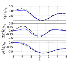
(a) $\,\,\epsilon_{1}=5\epsilon_{0}/12$

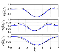
(b) $\,\epsilon_{1}=\epsilon_{0}/2$

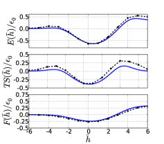
(c) $\,\epsilon_{1}=7\epsilon_{0}/12$

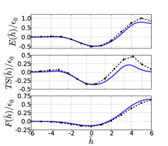
(d) $\,\epsilon_{1}=8\epsilon_{0}/12$

Figure 3: Profiles of the energy, entropy, and the free energy as a function of $\bar{h}$ for various values of $\epsilon_{1}$ at $T=\epsilon_{0}/3.6k_{B}$. The blue lines were calculated from Eq. 6, while the dashed black lines with squares were obtained from simulations.

$$Z_{pinned}(\bar{h})\approx b^{2}\frac{e^{2aL}}{2\pi aL}e^{-(\bar{h}-1)^{2}/aL}\,,$$ (15)

where

$$b\equiv e^{-2a}\left[e^{\beta(3\epsilon_{1}/2-\epsilon_{0}/2)}e^{(-2\bar{h}+1)/(2aL)}+e^{\beta(\epsilon_{1}/2)}+e^{\beta((\epsilon_{1}-\epsilon_{0})/2)}e^{(2\bar{h}-3)/(2aL)}\right]\,,$$ (16)

Using Eqs. 6,8,11,15, we can readily obtain profiles of free energy $F(\bar{h})=-\beta^{-1}\ln Z(\bar{h})$, energy $E(\bar{h})=-(\partial\ln Z(\bar{h})/\partial\beta)_{L}$, and entropy $S(\bar{h})=(E-F)/T$. These analytical results are plotted in Fig. 3 for a lattice of size $L=30$, at temperature $T=\epsilon_{0}/3.6k_{\rm B}$, and for various values of $\epsilon_{1}/\epsilon_{0}$. They agree very well with simulation results. In particular, the depth of minima at $\bar{h}=0$ are accurately predicted. In Fig. 4 we focus on these adsorption properties, $\Delta g_{ads}\equiv g(0)-g(-(L-1)/2)$ for thermodynamic property $g$, for the specific case $\epsilon_{1}=\epsilon_{0}/2$ . Theoretical predictions are plotted as functions of temperature at $L=30$ alongside results of Monte Carlo simulations.

Agreement is very good for temperatures in the range $\epsilon_{0}/6k_{B}<T<\epsilon_{0}/3k_{B}$ for $L=30$.

The failure of our theory at high temperature stems from neglect of contributions to $Z$ from terms of order $O(a^{2})$ and higher. At high temperature ruggedness of the interface can also render the RSOS model a poor proxy for the SOS model. At higher temperatures still, neglect of bulk inhomogeneities in the SOS model is itself not justified. At low temperatures a different prerequisite for the validity of Eq. 5 is violated, namely, $aL$ is no longer a large number. For the RSOS fluid with $L=30$ columns, $aL\approx 1$ when $T\approx 0.147\epsilon_{0}/k_{B}$. For temperatures around or lower than this value, height fluctuations in the RSOS fluid are no longer Gaussian to a good approximation.

Success of the SOS approximation in the temperature range $\epsilon_{0}/6k_{B}<T<\epsilon_{0}/3k_{B}$ reveals clearly the source of entropy variations observed in our lattice gas simulations. Absent density fluctuations in the liquid or vapor phase (which are neglected in the SOS description), fluctuations in interfacial shape provide the sole source of entropy in these schematic models. The minimum in $S(\bar{h})$ near $\bar{h}=0$ thus directly indicates suppression of capillary fluctuations when the solute resides at the liquid-vapor interface. Similarly, local maxima of $S(\bar{h})$ just above and below $\bar{h}=0$ signify enhancement of surface undulations when the solute pulls the interface a few lattice spacings away from its natural equilibrium position.

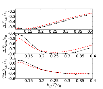
Figure 4: Free energy, energy, entropy of adsorption as a function of $T$ for $\epsilon_{1}=\epsilon_{0}/2$, with $L=30$. The red line is calculated from theory, while the black line with circles is obtained from simulations.

Interfacial pinning is strongest for a solute with coupling constant $\epsilon_{1}\approx\epsilon_{0}/2$. In simulations this conclusion is suggested by the depth of entropy minima at $\bar{h}=0$, which are most pronounced at intermediate coupling. It can be drawn more directly in our RSOS theory from the statistical weight $P_{pinned}(\bar{h})=Z_{pinned}(\bar{h})/Z(\bar{h})$ of the pinned subensemble. For a given value of $\epsilon_{1}$, $P_{pinned}(\bar{h})$ is always greatest at $\bar{h}=0$, where pinning does not require deforming the interface. (See Fig. 5) $P_{pinned}(0)$ should clearly increase with $\epsilon_{1}$ in the strongly solvophobic regime, where weak attraction to solvent is insufficient to offset the entropic price of suppressing capillary-like waves. It is also clear that $P_{pinned}(0)$ should decrease with $\epsilon_{1}$ in the strongly solvophilic regime, where extremely favorable solvation encourages the fluctuating interface to deform above a solute at $\bar{h}=0$ (i.e., to remain in the in state). Fig 5 bears out the resulting expectation that pinning is most effective at intermediate $\epsilon_{1}$, very close to $\epsilon_{1}=\epsilon_{0}/2$.

Subensemble weights $P_{\alpha}(\bar{h})\equiv Z_{\alpha}(\bar{h})/Z(\bar{h})$, where $\alpha=\{in,out,pinned\}$ , also shed light on the nature of entropy maxima at values of $\bar{h}$ a few lattice spacings above and below the GDS. In the RSOS model the total entropy can be decomposed by subensemble:

$$S(\bar{h})=\sum_{\alpha}S_{\alpha}(\bar{h})P_{\alpha}(\bar{h})-k_{B}\sum_{\alpha}P_{\alpha}(\bar{h})\ln P_{\alpha}(\bar{h})\,,$$ (17)

where $S_{\alpha}=(E_{\alpha}-F_{\alpha})/T$ characterizes fluctuations within each subensemble. The final term in Eq. 17 is an entropy of mixing associated with fluctuations between in, out, and pinned states. Plots of $P_{\alpha}(\bar{h})$ in Fig. 5 show that in and pinned states become about equally probable near $\bar{h}=-2$, contributing a mixing entropy of roughly $k_{\rm B}\ln 2$. This gain is partially offset by the intrinsically low entropy of the pinned state, and by decreasing $S_{in}$ as the requirement $h_{s}>\bar{h}$ becomes a nonnegligible constraint on interfacial fluctuations in the solvated state. The residual increase in entropy is a signature of spontaneous switching from the pinned state to an unpinned state, and vice versa. Analogous switching between pinned and unsolvated states is responsible for the entropy maximum at $\bar{h}=+4$.

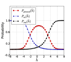
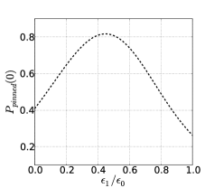
Figure 5: (a) Probabilities of the pinned, in, and out states as a function of $\bar{h}$ for $T=\epsilon_{0}/3.6k_{B}$, $\epsilon_{1}/\epsilon_{0}=1/2$ and (b) probability of the pinned state at $\bar{h}=0$ as a function of $\epsilon_{1}$ for $T=\epsilon_{0}/3.6k_{B}$. When the solute is near the GDS at $\bar{h}=0$, most of the configurations are in the pinned state.

Energy can also be decomposed by subensemble:

$$E(\bar{h})=\sum_{\alpha}E_{\alpha}(\bar{h})P_{\alpha}(\bar{h})\,,$$ (18)

where $E_{\alpha}(\bar{h})$ is the average energy in subensemble $\alpha$ when the solute is held at $\bar{h}$. Eqs 4, 9, 12, allow rough estimates of $E_{\alpha}(\bar{h})$ and thus simple predictions for energies of adsorption. For $\bar{h}\gg 0$ the unsolvated state dominates ($P_{out}=1$), giving $E(\infty)\approx E_{out}\approx E_{0}$, where $E_{0}$ is the average energy of the solute-free system. For $\bar{h}\ll 0$ the solvated state dominates ($P_{in}=1$), giving $E(-\infty)\approx E_{in}\approx E_{0}-4(\epsilon_{1}-\epsilon_{0}/2)$ from Eq. 9. To the extent that pinning dominates at $\bar{h}=0$, we have $E(0)\approx E_{pinned}(0)\approx E_{0}+\Delta H(h_{s-1},h_{s+1};\bar{h})$. At temperatures low enough to safely set $h_{s-1}=h_{s+1}=\bar{h}$ for the pinned state, we have $E(0)\approx E_{0}-3\epsilon_{1}-\epsilon_{0}$. Interfacial adsorption of the solute from the liquid phase therefore produces an energy change $E(0)-E(-\infty)\approx\epsilon_{1}-\epsilon_{0}$, accounting roughly for replacing a solvent-solute bond with a solvent-solvent bond. For a modestly solvophilic solute ($\epsilon_{0}/2<\epsilon_{1}<1)$, adsorption is energetically favorable, and the energetic driving force strengthens with decreasing $\epsilon_{1}$. This force is stronger still in the solvophobic regime ($\epsilon_{1}<\epsilon_{0}/2$), but these solutes reside primarily in the vapor phase. The strongest relevant energy of adsorption from the liquid phase is thus obtained for $\epsilon_{1}\approx\epsilon_{0}/2$, for which $\Delta E_{ads}\approx-\epsilon_{0}/2$.

These crude predictions are consistent at low temperatures (below $T=0.15\,\epsilon_{0}/k_{B}$ for $L=30$) with results from our simulations and detailed theoretical analysis (see Fig. 4). At temperatures above $T=0.15\,\epsilon_{0}/k_{B}$ for a lattice of size $L=30$, interfacial fluctuations modify $\Delta E_{ads}$ significantly. Reduced coordination at a rough interface enhances the energetic driving force for adsorption, effectively increasing the number of solvent-solute and solvent-solvent bonds exchanged when the solute moves to the surface (see Fig. 4). At the same time, however, the opposing entropic forces discussed above become more pronounced as temperature increases. It is not obvious from our simple estimates how this competition plays out, though the sign and magnitude of $\Delta S_{ads}$ ensures that net surface propensity decreases smoothly with increasing temperature (see Fig. 4). Regardless of temperature, adsorption is always strongest when $\epsilon_{1}=\epsilon_{0}/2$ (see Fig. 6).

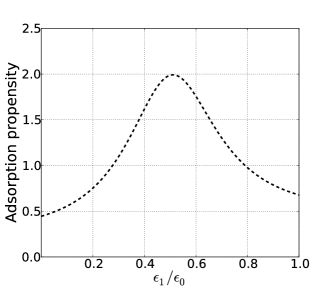
Figure 6: Adsorption propensity defined as $\frac{Z(0)}{Z({-(L-1)}/{2})+Z({(L-1)}/{2})}$ as a function of $\epsilon_{1}$ for $T=\epsilon_{0}/3.6k_{B}$. These estimates were calculated using Eq. 6.

V Conclusions

Among models that resolve microscopic fluctuations of the liquid-vapor interface, the two-dimensional lattice gas we have studied may be the simplest from which mechanisms of solute surface propensity might be learned. Any insight it offers into the behavior of real molecular systems is no doubt schematic. But the fact that it captures thermodynamic trends which elude celebrated theories of solvation encourages a detailed view of its conclusions in the context of more realistic molecular models.

Any such comparison requires assigning interaction parameters $\epsilon_{0}$ and $\epsilon_{1}$ to systems with much more complicated energetics. We do so through the local approximation of Eq. 1, which for simulations accurately describes the potential energy of a non-polarizable ion in water at a level of detail akin to that of a lattice gas. For a three-dimensional lattice gas model of bulk solvent, the total energy could be calculated by attributing to each liquid cell half of the interactions with its 6 neighboring liquid cells, so that $\epsilon_{bulk}=-3\epsilon_{0}$ (neglecting solvent density inhomogeneities). Similarly, since solvent cells at an ideally flat liquid-vapor interface engage in one fewer interaction than in bulk, we estimate $\epsilon_{interface}\approx-(5/2)\epsilon_{0}$. From the value of $\epsilon_{interface}-\epsilon_{bulk}=6.52$ kJ/mol computed from atomistic simulations of water Otten et al. (2012), we thus infer a coarse-grained solvent-solvent attraction strength $\epsilon_{0}\approx 13.04$ kJ/mol. Within the local approximation, solvent cells adjacent to the solute would be assigned half of their solvent-solvent interactions as well as a single solute bond. For a solute well within bulk solution, we then have $\epsilon_{coord}=-\epsilon_{1}-(5/2)\epsilon_{0}$ in the absence of solvent density inhomogeneities (i.e., within the SOS approximation). From the value $\epsilon_{coord}-\epsilon_{bulk}=-4.44$ kJ/mol determined for a fractionally charged non-polarizable Iodine ion in water, I^-0.8, by simulation Otten et al. (2012) we finally obtain $\epsilon_{1}=10.96$ kJ/mol, or $\epsilon_{1}/\epsilon_{0}\approx 0.84$.

From a lattice gas perspective, the simulated solute I^-0.8 (aq) therefore falls within the hydrophilic regime $\epsilon_{1}/\epsilon_{0}>1/2$. Further reducing the magnitude of the solute’s charge should certainly weaken solute-solvent attractions. Decreasing $\epsilon_{1}$ by a small amount in this way should bring the solute closer to conditions of maximum adsorption, $\epsilon_{1}=\epsilon_{0}/2$, where the scales of adsorption energy and entropy are both largest. Based on results we have presented, we thus expect that changing the ion’s charge from $-0.8e$ to $-0.75e$ would deepen the interfacial minima of energy and entropy profiles. Using the same molecular simulation techniques described in Ref. Otten et al. (2012), we find this prediction to indeed hold true.

In drawing this comparison we have assumed that basic interfacial solvation properties of the lattice gas are insensitive to dimensionality $d$. Although scaling behavior of a lattice gas near the critical point is famously sensitive to $d$, there is good reason to expect that the essence of our conclusions regarding solvation will be unchanged when moving from $d=2$ to $d=3$. The liquid-vapor interface of a three-dimsional lattice gas similarly supports capillary wave-like fluctuations for temperatures in the range $T_{R}<T<T_{c}$, where $T_{R}$ denotes the so-called roughening transition temperature Weeks et al. (1973). Furthermore, these surface undulations are Gaussian distributed to a good approximation at long wavelengths Vaikuntanathan et al. (2012); Weeks (1977), just as in Eq. 5. Partition functions of the in, out, and pinned states should therefore have similar forms in $d=3$. In qualitative terms, only the scale of height fluctuations governing $Z_{in}$, $Z_{out}$, and $Z_{pinned}$ will change, growing with system size only as $\sqrt{\ln L}$ rather than $\sqrt{L}$  Safran (2003). Preliminary simulation results for the $d=3$ case bear out these expectations.

We conclude that lattice gas models of interfacial solvation are a promising starting point for scrutinizing essential effects of surface roughness and energetic heterogeneity on solute adsorption. For the especially interesting case of charged solutes in highly polar solvents, a more realistic treatment of electrostatics is clearly in order. Given the success of lattice models for dielectric response  Song and Chandler (1998), this improvement appears quite feasible. An ability to treat solutes of varying size and geometry would also greatly aid connections with experiment. These developments are underway.

Appendix A Appendix

Here we present arguments underlying the assertion that a solute with coupling constant $\epsilon_{1}=\epsilon_{0}/2$ is equally likely to reside in either bulk phase. Consider a pair of configurations $\{n_{i},n_{i}^{s}\}$ and $\{n_{i}^{\prime},n_{i}^{s}\}$ related by a global transformation that swaps liquid and vapor phases. Specifically, the configuration $\{n_{i}^{\prime},n_{i}^{s}\}$ is obtained from $\{n_{i},n_{i}^{s}\}$ by changing the solvent occupation state of all lattice cells not occupied by the solute, $n_{i}^{\prime}=(1-n_{i}^{s})(1-n_{i})$. Repeating this transformation, $n_{i}=(1-n_{i}^{s})(1-n_{i}^{\prime})$, we recover the original configuration $\{n_{i},n_{i}^{s}\}$. In simple terms, if the solute resides in the liquid phase in $\{n_{i},n_{i}^{s}\}$, then it resides in the vapor phase in $\{n_{i}^{\prime},n_{i}^{s}\}$, and vice versa.

With an accompanying transformation of the solute-solvent coupling $\epsilon_{1}$, the energies of configurations $\{n_{i},n_{i}^{s}\}$ and $\{n_{i}^{\prime},n_{i}^{s}\}$ can be directly related. Defining $E(\{n_{i},n_{i}^{s}\};\{\epsilon_{0},\epsilon_{1}\})$ as the energy of configuration $\{n_{i},n_{i}^{s}\}$ with solvent-solvent coupling $\epsilon_{0}$, and solvent-solute coupling $\epsilon_{1}$, we have

$$\begin{split}E(\{n_{i}^{\prime},n^{s}_{i}\};\{\epsilon_{0},\epsilon_{1}\})&=-{\epsilon_{0}}\sum_{i,j\in nn}n_{i}^{\prime}n_{j}^{\prime}-\mu\sum_{i}n_{i}^{\prime}-\epsilon_{1}\sum_{i,j\in nn}n^{s}_{i}n_{j}^{\prime}\quad\\ &=-{\epsilon_{0}}\sum_{i,j\in nn}n_{i}n_{j}-\mu\sum_{i}n_{i}-(\epsilon_{0}-\epsilon_{1})\sum_{i,j\in nn}n^{s}_{i}n_{j}+4(\epsilon_{1}-\epsilon_{0}/2)\\ &=E(\{n_{i},n^{s}_{i}\};\{\epsilon_{0},\epsilon_{0}-\epsilon_{1}\})+4(\epsilon_{1}-\epsilon_{0}/2).\end{split}$$ (19)

When $\epsilon_{1}=\epsilon_{0}/2$, the energy of the two configurations are the same. Thus for every configuration in which the solute is in the liquid phase, there exists a configuration with the same statistical weight in which the solute is in the vapor phase and vice versa. Hence solutes with $\epsilon_{1}=\epsilon_{0}/2$ exhibit equal preference for the liquid and vapor phases.

References

- Jungwirth and Tobias (2006) P. Jungwirth and D. J. Tobias, Chem. Rev., 2006, 106, 1259–1281.
- Jungwirth and Tobias (2002) P. Jungwirth and D. Tobias, The Journal of Physical Chemistry B, 2002, 106, 6361–6373.
- Petersen and Saykally (2004) P. Petersen and R. Saykally, Chemical Physics Letters, 2004, 397, 51–55.
- Noah-Vanhoucke and Geissler (2009) J. Noah-Vanhoucke and P. Geissler, Proceedings of the National Academy of Sciences, 2009, 106, 15125–15130.
- Otten et al. (2012) D. Otten, P. Shaffer, P. Geissler and R. Saykally, Proceedings of the National Academy of Sciences, 2012, 109, 701–705.
- Onsager and Samaras (1934) L. Onsager and N. Samaras, The Journal of Chemical Physics, 1934, 2, 528.
- Archontis and Leontidis (2006) G. Archontis and E. Leontidis, Chemical Physics Letters, 2006, 420, 199–203.
- Levin (2009) Y. Levin, Physical Review Letters, 2009, 102, 147803.
- Levin et al. (2009) Y. Levin, A. P. D. Santos and A. Diehl, Physical Review Letters, 2009, 103, 257802.
- Markin and Volkov (2002) V. Markin and A. Volkov, The Journal of Physical Chemistry B, 2002, 106, 11810–11817.
- Huang and Chandler (2002) D. M. Huang and D. Chandler, The Journal of Physical Chemistry B, 2002, 106, 2047–2053.
- Caleman et al. (2011) C. Caleman, J. Hub, P. van Maaren and D. van der Spoel, Proceedings of the National Academy of Sciences, 2011, 108, 6838.
- Iuchi et al. (2009) S. Iuchi, H. Chen, F. Paesani and G. A. Voth, The Journal of Physical Chemistry B, 2009, 113, 4017–4030.
- Stuart and Berne (1996) S. Stuart and B. Berne, The Journal of Physical Chemistry, 1996, 100, 11934–11943.
- Vaitheeswaran and Thirumalai (2006) S. Vaitheeswaran and D. Thirumalai, Journal of the American Chemical Society, 2006, 128, 13490–13496.
- Weeks (1977) J. Weeks, The Journal of Chemical Physics, 1977, 67, 3106.
- Chui and Weeks (1981) S. Chui and J. Weeks, Phys. Rev. B, 1981, 23, 2438.
- Abraham (1980) D. B. Abraham, Phys. Rev. Lett., 1980, 44, 1165–1168.
- Fisher (1984) M. Fisher, Journal of Statistical Physics, 1984, 34, 667–729.
- Nelson et al. (2004) D. Nelson, T. Piran and S. Weinberg, Statistical Mechanics of Membranes and Surfaces, World Scientific Pub., 2004.
- Temperley (1952) H. N. V. Temperley, Mathematical Proceedings of the Cambridge Philosophical Society, 1952, 683–697.
- Safran (2003) S. Safran, Statistical Thermodynamics Of Surfaces, Interfaces, And Membranes, Westview Press, 2003.
- Kardar (2007) M. Kardar, Statistical Physics of Fields, Cambridge University Press, 2007.
- Weeks et al. (1973) J. Weeks, G. Gilmer and H. Leamy, Physical Review Letters, 1973, 31, 549–551.
- Vaikuntanathan et al. (2012) S. Vaikuntanathan, P. Shaffer and P. L. Geissler, Unpublished, 2012.
- Song and Chandler (1998) X. Song and D. Chandler, The Journal of Chemical Physics, 1998, 108, 2594–2600.