Symmetry-breaking Effects for Polariton Condensates in Double-Well Potentials

Abstract

We study the existence, stability, and dynamics of symmetric and anti-symmetric states of quasi-one-dimensional polariton condensates in double-well potentials, in the presence of nonresonant pumping and nonlinear damping. Some prototypical features of the system, such as the bifurcation of asymmetric solutions, are similar to the Hamiltonian analog of the double-well system considered in the realm of atomic condensates. Nevertheless, there are also some nontrivial differences including, e.g., the unstable nature of both the parent and the daughter branch emerging in the relevant pitchfork bifurcation for slightly larger values of atom numbers. Another interesting feature that does not appear in the atomic condensate case is that the bifurcation for attractive interactions is slightly sub-critical instead of supercritical. These conclusions of the bifurcation analysis are corroborated by direct numerical simulations examining the dynamics of the system in the unstable regime.

I Introduction

Over the past few years, a novel direction in the study of Bose-Einstein condensation has captured a considerable amount of attention. This concerns the observation of exciton-polariton Bose-Einstein condensates (BECs) in semiconductor microcavities kasp1_and_more ; balili ; lai ; deng . A fundamental feature of these exciton-polariton BECs is that, upon confinement, the excitons (bound pairs of electrons and holes) couple strongly to the incident light creating the polariton quasi-particles micro_cavity_polaritons . The resulting exciton-polariton BEC possesses a number of remarkable properties that we briefly touch upon below.

The radiative lifetime of the polaritons is the shorter relaxation time scale of the system being of the order of 1–10 ps benoit . On the other hand, the light mass of the exciton-polaritons provides this system with a significantly higher condensation temperature. The photonic component of the exciton-polaritons is responsible for their short lifetime which, in turn, does not allow thermalization; instead, it produces a non-equilibrium condensate, wherein the presence of external pumping from an exciton reservoir is critical towards a counter-balance of the polariton loss. In such genuinely non-equilibrium condensates, numerous remarkable features have been not only theoretically predicted but also experimentally established; these include the flow without scattering (analog of the flow without friction) amo1 , the existence of vortices lagou1 (see also Ref. roumpos for vortex dipole dynamics and Ref. roumpos1 for observations thereof), the collective dynamics amo2 , as well as remarkable applications such as spin switches amo3 and light emitting diodes amo4 operating even near room temperatures.

Perhaps the most customary approach to modeling exciton-polariton BECs involves the coupling of the evolution of the polaritons to that of the exciton reservoir which enables their production (and which features diffusive spatial dynamics of the excitons); this way, the model takes the form of two coupled complex Ginzburg-Landau (cGL) equations describing the evolution of exciton and photon wavefunctions polar1 ; polar2 ; cc05 . Nevertheless, it has been proposed in Refs. berloff1 ; kbb ; review_nb that a single cGL equation for the macroscopically occupied polariton state can also be used in a way consistent with experimental observations nbb_nature . A similar approach was followed in Ref. magnons where a BEC of magnon quasi-particles, incorporating a source term rather than an amplification of the field, was shown to be phenomenologically described by a system two nonlinearly coupled cGL-type equations. In the context of the single cGL model for the polaritons, there exists a localized (pumping) region of gain and a nonlinear saturating loss term, in addition to all the standard terms (quantum pressure, external parabolic trapping and repulsive interatomic interaction) that one encounters in atomic BECs emergent . Furthermore, it should be pointed out that the prototypical setting where experiments have been conducted is two-dimensional in nature. Yet, highly anisotropic traps (similar to what has been done in atomic BECs emergent ) can be envisioned which reduce the effective dynamics to a quasi one-dimensional (1D) setting 1d_polaritons1 ; 1d_polaritons2 ; 1d_polaritons3 ; 1d_polaritons4 ; 1d_polaritons5 ; 1d_polaritons6 . Moreover, recent experimental advances have enabled the use of thin microwires in order to guide the condensates along the direction of the wire Amo:10 . In this setting, the recent analysis of Ref. augusto presented a number of striking characteristics due to the interplay of gain and loss terms with the standard ones of atomic BECs. Prominent examples included the destabilization of the nodeless state of the system and the creation of stability inversions (where states with nodes would be more robust), as well as the existence of bubble-like and sawtooth-like solutions in the system.

A very interesting research direction in the physics of atomic and polariton BECs concerns the dynamics of the condensates in a double-well potential. The latter can be created in atomic BEC experiments through the combination of a parabolic trap and a periodic (so-called optical lattice) potential generated through the interference of laser beams illuminating the BEC Morsch . Relevant experiments in atomic BECs markus1 ; markus2 have paved the way towards the exploration of numerous features such as tunneling and Josephson oscillations for small numbers of atoms in the condensate, and macroscopic quantum self-trapped states, as well as symmetry-breaking effects for large atom numbers. On the other hand, double-well potentials can also be created in polariton BEC experiments in microcavities by applying stress balili ; balapl , by employing photolithographic techniques 1d_polaritons1 ; 1d_polaritons2 , or allowing natural formation during the sample growth lagdw . Importantly, the latter technique was used for the study of a “polariton Josephson junction” lagdw , in the spirit of earlier studies on “bosonic Josephson junctions” rudi in the context of atomic BECs. Importantly, a large volume of theoretical studies has accompanied these developments, first in the context of atomic BECs, through investigations related to finite-mode reductions and symmetry-breaking bifurcations smerzi ; kiv2 ; mahmud ; bam ; Bergeman_2mode ; infeld ; todd ; TKF06 , quantum effects carr , and nonlinear variants of the double-well potential pseudo , and more recently in the context of polariton condensates, especially as concerns Josephson oscillations therein polardw . It should be mentioned in passing that similar (spontaneous symmetry breaking) effects have been monitored in the realm of nonlinear optics: in this context, formation of asymmetric states in dual-core fibers fibers , self-guided laser beams in Kerr media HaeltermannPRL02 , and optically-induced dual-core waveguiding structures in photorefractive crystals zhigang have been reported.

It is the aim of the present work to combine these two themes, namely the focus on the exciton-polariton BEC with pumping and loss and the fundamental interest in the understanding of double-well trapping potentials in a spirit similar to the proposal of Ref. polar1 . In particular, we will consider the single-component model of Refs. berloff1 ; kbb ; review_nb combined with a double-well potential in a quasi-1D (e.g., microwire) setting. We will attempt a systematic (Galerkin) finite-dimensional reduction of the system via projection to the two principal eigenstates of the potential, and will derive a damped-driven system of ordinary differential equations (ODEs) that have been shown in the Hamiltonian case to capture the essence of the statics kirr and dynamics marzuola of double-well potentials. We will then examine the bifurcation structure of the resulting ODEs and compare it to that of the original partial differential equation (PDE) model. This already provides us with a number of interesting features that distinguish this system from its Hamiltonian analog. For instance, in the case of attractive interatomic interactions (which is studied together with that of repulsive interactions) the relevant symmetry-breaking pitchfork bifurcation is subcritical instead of supercritical as in the Hamiltonian case. Furthermore, both branches that emerge from the pitchfork bifurcations, the stable asymmetric one and the (now) unstable “parent” branch, both appear to become destabilized in this polariton BEC setting for slightly larger nonlinearities, posing the natural question of what is the stable dynamics for larger values of the nonlinearity. These questions will in part be addressed via direct numerical simulations.

Our presentation will be structured as follows. First, in Section II, we will present the model and its theoretical study via the Galerkin analysis. In Section III, we will study the model numerically and compare the results of the numerical bifurcation analysis with the prediction of the Galerkin approximation. We will also complement these results with direct numerical simulations of the original model. Finally, in section IV, we summarize our results and present our conclusions.

II Model setup and analytical predictions

In our analysis below, we adopt the model of Refs. berloff1 ; kbb ; review_nb . It has been argued in these works that the original exciton-polariton system given by a set of two coupled equations can be effectively reduced to a single cGL equation with a nonlinear saturating loss term. This reduction can be used when the reservoir mean-field potential is negligible and the spot size is large compared with the condensate size (i.e., if we can consider that the spot width is the same of the spatial extent of the system). In particular, the amplification of the existing field introduces a gain and hence acts as a generator of polaritons. Then the loss term saturates this gain beyond a certain threshold. These two terms are analogous to the pumping of polaritons from the excitons and to the natural decay of the polaritons. This reduced model can be expressed in dimensionless form as follows:

$$i\partial_{t}u=-\partial_{x}^{2}u+s|u|^{2}u+V(x)u-\mu u+i\left[\chi(x)-\sigma|u|^{2}\right]u.$$ (1)

The above model is actually a complex Ginzburg-Landau equation aranson for the complex order parameter $u(x,t)$, which is assumed to evolve in the presence of the effectively-1D double-well potential $V(x)$. Equation (1) can be applied to both the contexts of atomic and polariton BECs: in the first case, the two last terms in the right-hand side of Eq. (1) are absent, and the model —known as the Gross-Pitaevskii equation emergent — describes the evolution of the macroscopic wavefunction for the cold atoms and $\mu$ is the chemical potential; in the second case, $u(x,t)$ denotes the polariton wavefunction, and the last two terms in the right-hand side are included in the model. More specifically, in the context of polariton condensates, Eq. (1) incorporates (a) the spatially dependent gain term of the form

$$\chi(x)=\alpha\Theta(x_{m}-|x|),$$ (2)

where $\Theta$ is the step function generating a symmetric pumping spot of “radius” $x_{m}$ and strength $\alpha$ for the gain, and (b) a nonlinear saturation loss term, characterized by its strength $\sigma$. As concerns the parameter $s\equiv\pm 1$, it sets the type of nonlinearity (i.e., the type of interactions between atoms or polaritons): for $s=+1$ the nonlinearity is defocusing (i.e., the interactions are repulsive), while for $s=-1$ the nonlinearity is focusing (i.e., the interactions are attractive). In the context of atomic BECs, the value of $s$ depends on the atom species (e.g., $s=+1$ for ⁸⁷Rb or ²³Na, while $s=-1$ for ⁷Li or ⁸⁵Rb atoms). On the other hand, in the context of polariton condensates, the sign of the effective mass of polaritons [i.e., the sign of the first term in the right-hand side of Eq. (1)] may become either positive or negative, depending on the values of transverse momentum: in fact, the transition from positive to negative mass is associated with the inflection point of the energy-momentum diagram dvs . Here, we will consider both cases of $s=\pm 1$ to take into regard that the effective polariton mass may be positive or negative, respectively. We finally note that the relevant physical time and space scales, as well as physically relevant parameter values associated with Eq. (1), can be found in Ref. berloff1 .

In what follows, we will use the Galerkin (few mode truncation) approach of Ref. TKF06 . We start by considering the corresponding linear eigenproblem which reads:

$$Hu\equiv-\partial_{x}^{2}u+V(x)u=\omega u,$$ (3)

whose spectrum consists of a ground state, $u_{0}(x)$, and excited states, $u_{i}(x)$ (with $i\geq 1$). Then, in the weakly nonlinear regime, we consider a superposition of the two lowest linear eigenmodes,

$$u(x,t)=c_{0}(t)u_{0}(x)+c_{1}(t)u_{1}(x),$$ (4)

where $c_{0,1}(t)$ are unknown time-dependent complex prefactors; obviously, the above ansatz is relevant for values of the chemical potential $\mu$ such that higher order modes can be safely ignored. Substituting this ansatz into Eq. (1) we obtain:

$$i\left(\dot{c_{0}}u_{0}+\dot{c_{1}}u_{1}\right)=(\omega_{0}-\mu)u_{0}c_{0}+(\omega_{1}-\mu)u_{1}c_{1}+s|u|^{2}\left(c_{0}u_{0}+c_{1}u_{1}\right)+i\left[\chi(x)-\sigma|u|^{2}\right]\left(c_{0}u_{0}+c_{1}u_{1}\right),$$ (5)

where the $|u|^{2}$ has not been expanded only for reasons of compactness but should actually be thought as expanded according to Eq. (4). Next, projecting on $u_{0}$ and $u_{1}$ (i.e., multiplying the above equation by $u_{0}$ and $u_{1}$ and integrating over $x$), and using the orthogonality of the states $u_{i}$, we respectively derive the following equations:

$$i\dot{c_{0}}=(\omega_{0}-\mu+i\alpha_{0})c_{0}+(s-i\sigma)\left\{A_{0}|c_{0}|^{2}c_{0}+\left(c_{0}^{2}c_{1}^{*}+2|c_{0}|^{2}c_{1}\right)\Gamma_{0}+\left(2|c_{1}|^{2}c_{0}+c_{1}^{2}c_{0}^{*}\right)B+|c_{1}|^{2}c_{1}\Gamma_{1}\right\},$$ (6)

and

$$i\dot{c_{1}}=(\omega_{1}-\mu+i\alpha_{1})c_{1}+(s-i\sigma)\left\{\Gamma_{0}|c_{0}|^{2}c_{0}+\left(c_{0}^{2}c_{1}^{*}+2|c_{0}|^{2}c_{1}\right)B+\left(2|c_{1}|^{2}c_{0}+c_{1}^{2}c_{0}^{*}\right)\Gamma_{1}+|c_{1}|^{2}c_{1}A_{1}\right\}.$$ (7)

In the above equations, overdots denote time derivatives, the involved constants (depending on the eigenbasis $\{u_{i}\}$) take the values $A_{0}=\int u_{0}^{4}dx$, $A_{1}=\int u_{1}^{4}dx$, $B=\int u_{0}^{2}u_{1}^{2}dx$, $\Gamma_{0}=\int u_{1}u_{0}^{3}dx$, and $\Gamma_{1}=\int u_{0}u_{1}^{3}dx$, while the effective gain coefficients read: $\alpha_{0}=\int\chi(x)u_{0}^{2}dx$ and $\alpha_{1}=\int\chi(x)u_{1}^{2}dx$. We now use amplitude and phase variables for the time-dependent prefactors, i.e., $c_{i}=\rho_{i}e^{i\phi_{i}}$ (with the amplitudes $\rho_{i}$ and phases $\phi_{i}$ being real functions), to derive a set of four equations for the unknown functions $\rho_{0,1}$ and $\phi_{0,1}$. Introducing the relative phase of the first two modes as $\varphi\equiv\phi_{1}-\phi_{0}$, the above mentioned set of equations takes the following form:

$$\begin{split}\dot{\rho}_{0}=&\alpha_{0}\rho_{0}-\sigma\left(A_{0}\rho_{0}^{3}+2B\rho_{1}^{2}\rho_{0}\right)+s\left(\Gamma_{1}\rho_{1}^{3}+\Gamma_{0}\rho_{0}^{2}\rho_{1}\right)\sin\varphi\\ &+sB\rho_{1}^{2}\rho_{0}\sin 2\varphi-\sigma\left(\Gamma_{1}\rho_{1}^{3}+3\Gamma_{0}\rho_{0}^{2}\rho_{1}\right)\cos\varphi-\sigma B\rho_{1}^{2}\rho_{0}\cos 2\varphi,\end{split}$$ (8)

$$\begin{split}\dot{\phi_{0}}=&-(\omega_{0}-\mu)-s\left(A_{0}\rho_{0}^{2}+2B\rho_{1}^{2}\right)-\sigma\left(\Gamma_{0}\rho_{0}\rho_{1}+\Gamma_{1}{\rho_{1}^{3}}/{\rho_{0}}\right)\sin\varphi\\ &-\sigma B\rho_{1}^{2}\sin 2\varphi-s\left(3\Gamma_{0}\rho_{0}\rho_{1}+\Gamma_{1}{\rho_{1}^{3}}/{\rho_{0}}\right)\cos\varphi-sB\rho_{1}^{2}\cos 2\varphi,\end{split}$$ (9)

$$\begin{split}\dot{\rho}_{1}=&\alpha_{1}\rho_{1}-\sigma\left(A_{1}\rho_{1}^{3}+2B\rho_{0}^{2}\rho_{1}\right)-s\left(\Gamma_{0}\rho_{0}^{3}+\Gamma_{1}\rho_{1}^{2}\rho_{0}\right)\sin\varphi\\ &-sB\rho_{0}^{2}\rho_{1}\sin 2\varphi-\sigma\left(\Gamma_{0}\rho_{0}^{3}+3\Gamma_{1}\rho_{1}^{2}\rho_{0}\right)\cos\varphi-\sigma B\rho_{0}^{2}\rho_{1}\cos 2\varphi,\end{split}$$ (10)

and

$$\begin{split}\dot{\phi_{1}}=&-(\omega_{1}-\mu)-s\left(A_{1}\rho_{1}^{2}+2B\rho_{0}^{2}\right)+\sigma\left(\Gamma_{1}\rho_{1}\rho_{0}+\Gamma_{0}{\rho_{0}^{3}}/{\rho_{1}}\right)\sin\varphi\\ &+\sigma B\rho_{0}^{2}\sin 2\varphi-s\left(3\Gamma_{1}\rho_{1}\rho_{0}+\Gamma_{0}{\rho_{0}^{3}}/{\rho_{1}}\right)\cos\varphi-sB\rho_{0}^{2}\cos 2\varphi.\end{split}$$ (11)

Subtracting Eq. (9) from Eq. (11), we can readily obtain an equation for $\varphi$, namely:

$$\begin{split}\dot{\varphi}=&-\Delta\omega-s\left(A_{1}\rho_{1}^{2}-A_{0}\rho_{0}^{2}\right)-sB\left[2+\cos 2\varphi\right]\left(\rho_{0}^{2}-\rho_{1}^{2}\right)-s\frac{\cos\varphi}{\rho_{0}\rho_{1}}\left(\Gamma_{0}\rho_{0}^{2}(\rho_{0}^{2}-3\rho_{1}^{2})+\Gamma_{1}\rho_{1}^{2}(3\rho_{0}^{2}-\rho_{1}^{2})\right)\\ &+\sigma\frac{\sin\varphi}{\rho_{0}\rho_{1}}\left(\Gamma_{0}\rho_{0}^{2}(\rho_{0}^{2}+\rho_{1}^{2})+\Gamma_{1}\rho_{1}^{2}(\rho_{0}^{2}+\rho_{1}^{2})\right)+\sigma B\sin 2\varphi(\rho_{0}^{2}+\rho_{1}^{2}),\end{split}$$ (12)

where $\Delta\omega\equiv\omega_{1}-\omega_{2}$. This way, we have arrived to a system of three equations [cf. Eqs. (8), (10) and (12)] for the unknown functions $\rho_{0,1}$ and $\varphi$. These equations are subject to an additional constraint stemming from the balance condition $dN/dt=0$, where $N\equiv\int_{-\infty}^{+\infty}|u|^{2}dx$ is the number of polaritons (mathematically the squared $L^{2}$ norm). The evolution of the latter, can readily be found by multiplying Eq. (1) by $u^{*}$, the complex conjugate of Eq. (1) by $u$, and then adding and integrating the resulting equations. It is straightforward to find that the condition for equilibrium is:

$$\int_{-\infty}^{+\infty}\left(\chi(x)-\sigma|u|^{2}\right)|u|^{2}dx=0.$$ (13)

Substituting Eq. (4) into Eq. (13), also using the polar decomposition for $c_{i}(t)$ [and assuming a definite —even in our considerations— parity for the function $\chi(x)$], we find that the balance condition (13) takes the form:

$$\begin{split}\left(\alpha_{0}\rho_{0}^{2}+\alpha_{1}\rho_{1}^{2}\right)&-\sigma\left(A_{0}\rho_{0}^{4}+\rho_{1}^{4}A_{1}+4\rho_{0}^{2}\rho_{1}^{2}B\right)-4\sigma\left(\rho_{0}^{3}\rho_{1}\Gamma_{0}+\rho_{1}^{3}\rho_{0}\Gamma_{1}\right)\cos\varphi-2\sigma\rho_{0}^{2}\rho_{1}^{2}B\cos 2\varphi=0,\end{split}$$ (14)

which essentially fixes $\rho_{1}$ once $\rho_{0}$ and $\varphi$ are found and thus reducing the effective number of degrees of freedom for our approximations to only two ($\rho_{0}$ and $\varphi$).

Below, we will consider the case of a symmetric double-well potential, for which $\Gamma_{1}=\Gamma_{0}=0$. In this case, Eqs. (8), (10) and (12) are reduced to the following simpler form,

$$\begin{split}\dot{\rho}_{0}&=\alpha_{0}\rho_{0}-\sigma\left(A_{0}\rho_{0}^{3}+2B\rho_{1}^{2}\rho_{0}\right)+sB\rho_{1}^{2}\rho_{0}\sin 2\varphi-\sigma B\rho_{1}^{2}\rho_{0}\cos 2\varphi,\end{split}$$ (15)

$$\begin{split}\dot{\rho}_{1}&=\alpha_{1}\rho_{1}-\sigma\left(A_{1}\rho_{1}^{3}+2B\rho_{0}^{2}\rho_{1}\right)-sB\rho_{0}^{2}\rho_{1}\sin 2\varphi-\sigma B\rho_{0}^{2}\rho_{1}\cos 2\varphi,\end{split}$$ (16)

$$\begin{split}\dot{\varphi}&=-\Delta\omega-s\left(A_{1}\rho_{1}^{2}-A_{0}\rho_{0}^{2}\right)-sB\left[2+\cos 2\varphi\right]\left(\rho_{0}^{2}-\rho_{1}^{2}\right)+\sigma B\sin 2\varphi(\rho_{0}^{2}+\rho_{1}^{2}),\end{split}$$ (17)

while the equilibrium condition is accordingly simplified as:

$$\begin{split}\left(\alpha_{0}\rho_{0}^{2}+\alpha_{1}\rho_{1}^{2}\right)&-\sigma\left(A_{0}\rho_{0}^{4}+\rho_{1}^{4}A_{1}+4\rho_{0}^{2}\rho_{1}^{2}B\right)-2\sigma\rho_{0}^{2}\rho_{1}^{2}B\cos 2\varphi=0.\end{split}$$ (18)

We can now turn to the study of stationary solutions (i.e., $\dot{\rho}_{0}=\dot{\rho}_{1}=\dot{\varphi}=0$) resulting from the Galerkin truncation analysis. Particularly, from Eq. (15) we obtain two possible solutions:

$$\begin{cases}i)\quad\rho_{0}=0,\\ ii)\quad\alpha_{0}-\sigma\left(A_{0}\rho_{0}^{2}+2B\rho_{1}^{2}\right)+sB\rho_{1}^{2}\sin 2\varphi-\sigma B\rho_{1}^{2}\cos 2\varphi&=0,\end{cases}$$ (19)

while from Eq. (16) we obtain:

$$\begin{cases}i)\quad\rho_{1}=0\\ ii)\quad\alpha_{1}-\sigma\left(A_{1}\rho_{1}^{2}+2B\rho_{0}^{2}\right)-sB\rho_{0}^{2}\sin 2\varphi-\sigma B\rho_{0}^{2}\cos 2\varphi&=0.\end{cases}$$ (20)

Next, multiplying the nontrivial equilibria of Eq. (19) by $\rho_{0}^{2}$, the one from Eq. (20) by $\rho_{1}^{2}$, and adding the resulting equations, we obtain:

$$\cos 2\varphi=\frac{(\alpha_{0}\rho_{0}^{2}+\alpha_{1}\rho_{1}^{2})-\sigma\left(A_{0}\rho_{0}^{4}+A_{1}\rho_{1}^{4}+4B\rho_{0}^{2}\rho_{1}^{2}\right)}{2\sigma B\rho_{0}^{2}\rho_{1}^{2}},$$ (21)

while subtracting Eq. (20) from Eq. (19) yields:

$$\sigma\left(A_{1}\rho_{1}^{4}-A_{0}\rho_{0}^{4}+2B(\rho_{0}^{2}-\rho_{1}^{2})+B(\rho_{0}^{2}-\rho_{1}^{2})\cos 2\varphi\right)+sB(\rho_{0}^{2}+\rho_{1}^{2})\sin 2\varphi+(\alpha_{0}-\alpha_{1})=0.$$ (22)

Combining now Eq. (22) with Eq. (17) we finally obtain the result:

$$(\rho_{0}^{2}+\rho_{1}^{2})\sin 2\varphi=\frac{\sigma\Delta\omega-s(\alpha_{0}-\alpha_{1})}{B(\sigma^{2}+s^{2})}.$$ (23)

Let us now focus again on Eqs. (15) and (16): it is clear that if Eq. (16) is satisfied for $\rho_{1}=0$ then $\rho_{0}^{2}=\frac{\alpha_{0}}{\sigma A_{0}}$, and if Eq. (15) is satisfied with $\rho_{0}=0$ then $\rho_{1}^{2}=\frac{\alpha_{1}}{\sigma A_{1}}$. Aside from these trivial symmetric and anti-symmetric solutions, past the critical point for the symmetry breaking bifurcation, an asymmetric solution is expected to exist which possesses non-vanishing $\rho_{0}$ and $\rho_{1}$ (as well as a non-zero relative phase between them), which can be computed from Eq. (21). It is anticipated that the presence of loss and gain will not (generically) modify the nature of the bifurcations in comparison to the Hamiltonian case TKF06 . Namely, an asymmetric solution will bifurcate from the symmetric one in the focusing nonlinearity case of $s=-1$, due to a non-vanishing contribution of the anti-symmetric part in the solution, while on the contrary, an asymmetric mode will emanate from the anti-symmetric one in the defocusing nonlinearity setting of $s=1$ (due to a symmetric contribution within the solution). These results are detailed for a particular case example potential in what follows and compared to full numerical results.

III Numerical results

In our theoretical approximations, the double-well potential is constructed by placing a localized barrier at the center of the parabolic trap potential of strength $\Omega$. Particularly, the double-well potential is assumed to be of the form:

$$V(x)=\frac{1}{2}\Omega^{2}x^{2}+V_{0}\,\mathrm{sech}\left(\frac{x}{w}\right),$$ (24)

where $w$ is the width of the barrier and $V_{0}$ its height. The results presented below are for the potential parameters $\Omega^{2}=0.1$, $V_{0}=5$, and $w=0.2$; we have checked that other parameter values lead to quantitatively similar results . For the gain we consider a strength $\alpha=0.2$ and a spot size of $x_{m}=2.0$. The damping parameter $\sigma$ is used to vary the number of atoms, $N$, in order to do the continuation. For the above double-well potential, the values of the linear eigen-energies are $\omega_{0}=0.515729$ and $\omega_{1}=0.677697$. The potential setting under consideration is depicted in Fig. 1.

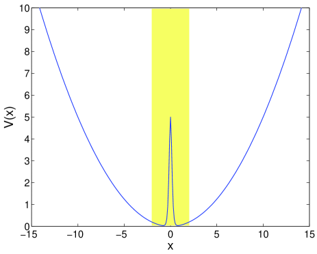
Figure 1: (Color online) The parabolic trapping potential and the localized barrier creating the double-well potential configuration. The parameter values used are: $\Omega^{2}=0.1$, $w=0.2$, and $V_{0}=5$; the shaded area corresponds to the region where the pumping acts, i.e., $|x|<x_{m}=2$.

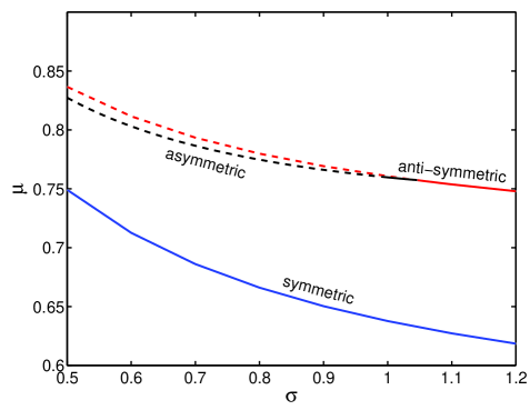
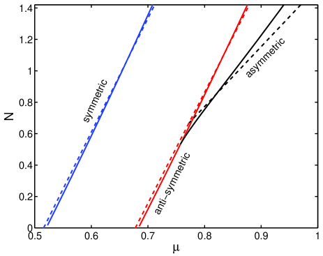
Figure 2: (Color online) Bifurcation diagrams for the symmetric, anti-symmetric and asymmetric branches for defocusing (repulsive) nonlinearity ($s=1$). Left: Dependence of the chemical potential on the damping parameter. Right: Dependence of the (normalized) number of polaritons on the chemical potential. Unstable solutions are depicted by dashed lines on the left panel. On the right solid lines display numerical results obtained by a nonlinear (Newton-Raphson) solver of the steady state equations of the model of Eq. (1), while dashed lines display analytical results of our Galerkin approach. The linear modes are located at $\mu=0.5157$ and $\mu=0.6667$.

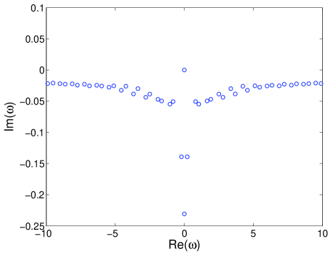
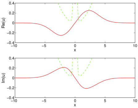
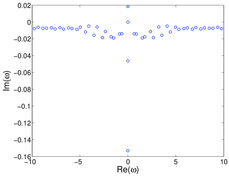
Figure 3: (Color online) (Left) Real and imaginary part of the wavefunction profile for a symmetric (top) and anti-symmetric (bottom) solution. (Right) Their corresponding stability eigenvalues. In all cases $\sigma=1$ and the interactions are repulsive ($s=+1$).

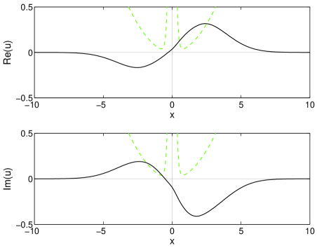
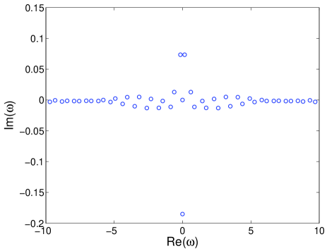
Figure 4: (Color online) (Left) Real and imaginary part of the wavefunction profile for an asymmetric solution with $\sigma=0.5$. (Right) Their corresponding stability eigenvalues. All cases correspond to the repulsive interaction case ($s=+1$).

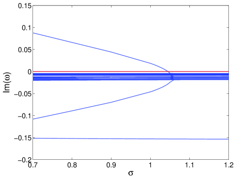
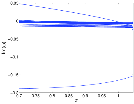
Figure 5: (Color online) Dependence of the imaginary part of the stability eigenvalues with respect to $\sigma$ for the anti-symmetric (left) and asymmetric solutions (right) in the repulsive interaction case ($s=+1$).

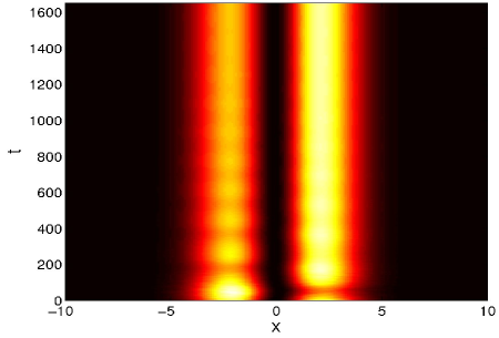
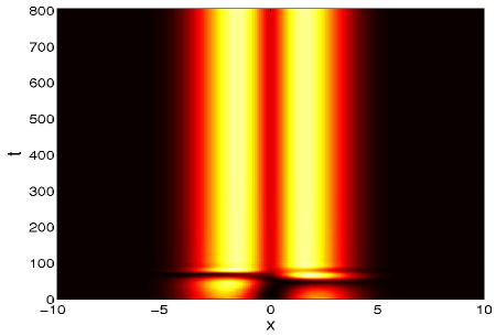
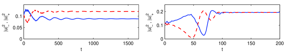
Figure 6: (Color online) Top: Evolution of a perturbed anti-symmetric soliton for $\sigma=1$ (left) and $\sigma=0.8$ (right) in the repulsive case ($s=+1$). The former case relaxes to the asymmetric stationary state, while the latter to the symmetric ground state. Bottom: Respective time series for the density at the bottom of the left (solid blue line) and right (dashed red line) wells.

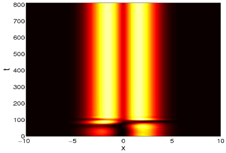
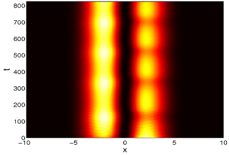
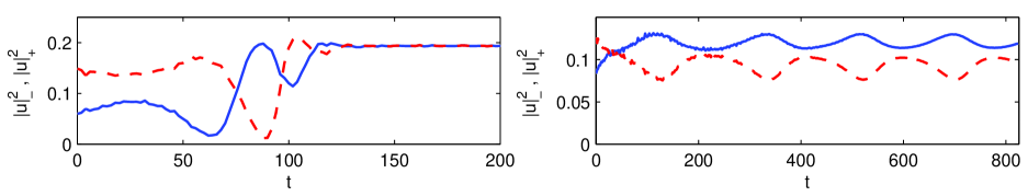
Figure 7: (Color online) Top: Evolution of a perturbed asymmetric soliton with $\sigma=0.8$ (left) and $\sigma=0.98$ (right) in the repulsive case ($s=+1$). In the former case, perturbation leads to the symmetric ground state attractor, while in the latter case, it relaxes to a non-stationary (quasi-periodic) solution. Bottom: Respective time series for the density at the bottom of the left (solid blue line) and right (dashed red line) wells.

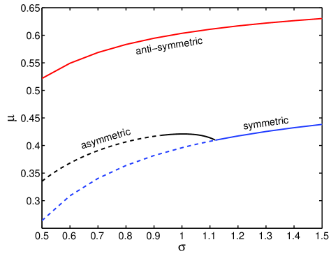
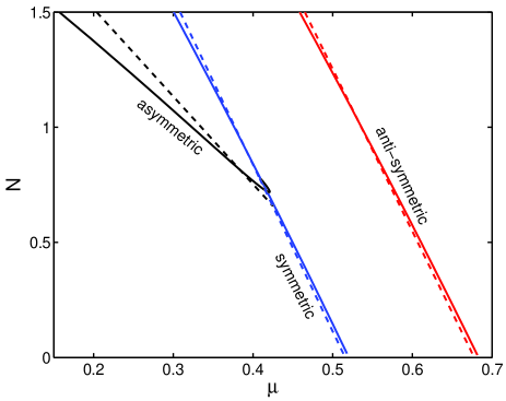
Figure 8: (Color online) Bifurcation diagrams for the symmetric, anti-symmetric and asymmetric branches for focusing (attractive) nonlinearity ($s=-1$). Left: Dependence of the chemical potential on the damping parameter. Right: Dependence of the (normalized) number of polaritons on the chemical potential. Unstable solutions are depicted by dashed lines on the left panel. On the right panel solid lines display numerical (Newton-Raphson) results, while dashed lines display analytical (Galerkin) results.

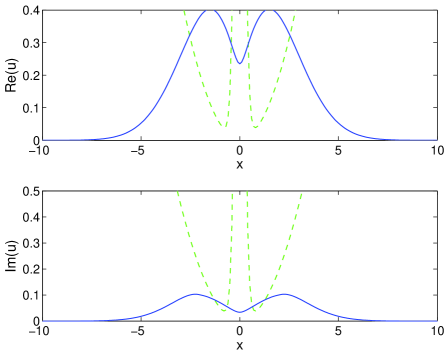
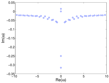
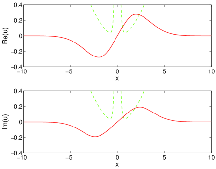
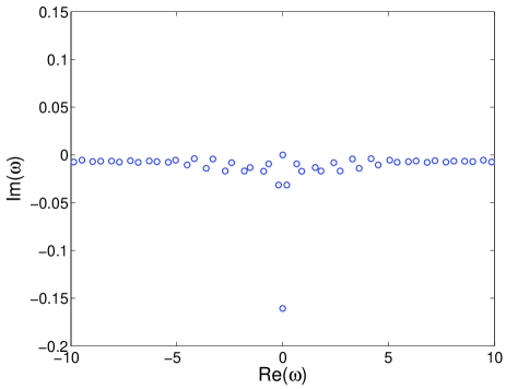
Figure 9: (Color online) (Left) Real and imaginary part of the wavefunction profile for a symmetric (top) and anti-symmetric (bottom) solution. (Right) Their corresponding stability eigenvalues. In all cases $\sigma=1$ and the nonlinearity is attractive ($s=-1$).

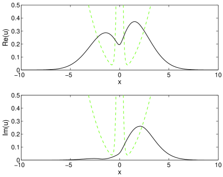
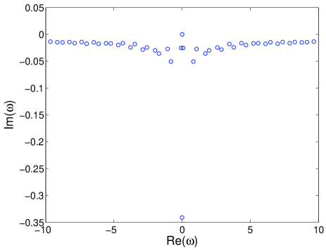
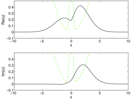
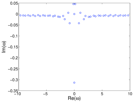
Figure 10: (Color online) (Left) Real and imaginary part of the wavefunction profile for an asymmetric solution with $\sigma=1$ (top) and $\sigma=0.7$ (bottom). (Right) Their corresponding stability eigenvalues. Notice the Hopf bifurcations and the associated oscillatory instabilities through two complex pairs which have occurred in the latter case. Here, the nonlinearity is attractive ($s=-1$).

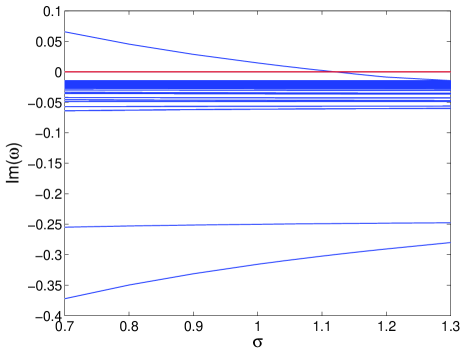
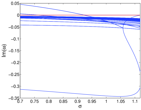
Figure 11: (Color online) Dependence of the imaginary part of the stability eigenvalues with respect to $\sigma$ for symmetric (left) and asymmetric solutions (right). Here, again, the nonlinearity is attractive ($s=-1$).

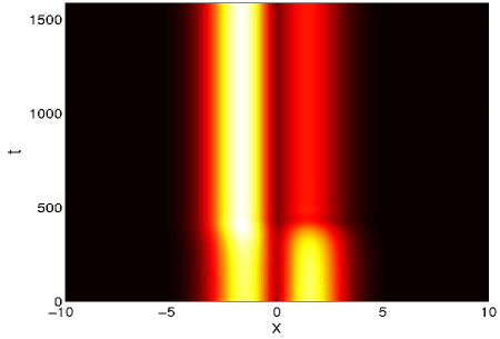
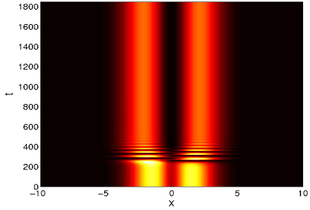
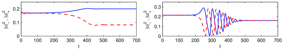
Figure 12: (Color online) Top: Evolution of perturbed symmetric solitons with $\sigma=1$ (left) and $\sigma=0.82$ (right) for attractive nonlinearity ($s=-1$). Bottom: Respective time series for the density at the bottom of the left (solid blue line) and right (dashed red line) wells.

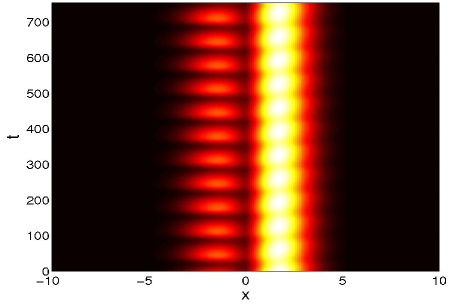
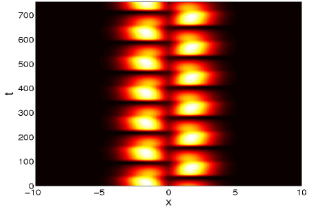
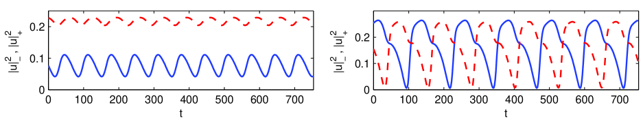
Figure 13: (Color online) Top: Dynamical evolution of the density of the non-stationary asymmetric solution branch found for attractive nonlinearity ($s=-1$) in two cases: $\sigma=0.9$ (left) and $\sigma=0.8$ (right). Bottom: Respective time series for the density at the bottom of the left (solid blue line) and right (dashed red line) wells.

We have performed a continuation of symmetric, anti-symmetric and asymmetric states in both cases of repulsive and attractive interactions. The continuations have been performed by increasing the damping parameter $\sigma$, which is tantamount to decreasing the norm or chemical potential. It is important to note that the chemical potential is no longer a free parameter in the present setting in sharp contrast to what is the case in the Hamiltonian regime of atomic BECs (see also the discussion of Refs. berloff1 ; augusto ). Similar results can be obtained by decreasing the pumping parameter $\alpha$. However, a crucial realization that emerges from considering variations of the different parameters is that the spot size $x_{m}$ must be chosen in a very limited range in order for the three above mentioned nonlinear modes to co-exist and be potentially stable; outside this range, instabilities lead to breathing multi-bump coherent structures. In what follows, the values of $x_{m}=2$ and $\alpha=0.2$ have been used unless explicitly indicated otherwise.

III.1 Repulsive case

We start by considering the case of the repulsive interaction with $s=+1$ (and vary $\sigma$ as mentioned above). The family of symmetric solutions is found to be always stable. As expected, on the other hand, and in agreement to our expectation from the realm of atomic BECs, the anti-symmetric solutions are exponentially unstable for small $\sigma$, which is tantamount to large polariton population numbers $N$. They become stable after the symmetry-breaking pitchfork bifurcation occurring at $\sigma=1.045$ (i.e., for $\mu<\mu_{cr}=0.7574$ and for $N<N_{cr}=0.5333$). The asymmetric branch that emerges through this bifurcation is stable for $\mu<0.7603$ and $N<0.5509$, i.e., for a narrow parametric interval past the bifurcation critical point. However, past this secondary critical point, the asymmetric solutions are prone towards an oscillatory instability emerging through a Hopf bifurcation (the critical loss strength in this case is $\sigma=0.989$). The relevant bifurcation diagrams are presented in Fig. 2, which shows the dependence of $\mu$ on $\sigma$, as well as the dependence of $N$ on $\mu$ (note that the latter form of the bifurcation diagram is more commonly used in relevant studies). The latter graph also contains the results of the theoretical analysis for the symmetric branch of Eq. (20) and for the anti-symmetric one of Eq. (19), as well as for the asymmetric branch which is theoretically predicted for the parameters of our double-well potential to bifurcate from the anti-symmetric solution for $\mu>0.7722$ and $N>0.6661$. As can be seen (also from Fig. 2), there is good agreement between theoretical predictions and numerical findings.

Some case examples of solution profiles for the different branches, together with the results of their corresponding linear stability analysis as performed by means of the Bogolyubov-de Gennes (BdG) ansatz emergent are shown in Figs. 3 and 4, The BdG analysis is represented by the spectral plane of the linearization eigenfrequencies $\omega={\rm Re}(\omega)+i{\rm Im}(\omega)$. Contrary to what is the case in the Hamiltonian setting of Ref. TKF06 (where the spectrum is chiefly on the imaginary axis), here the spectrum contains predominantly decaying modes with ${\rm Im}(\omega)<0$. For the stable symmetric ground state in Fig. 3, all modes are decaying except for the symmetry mode associated with $\omega=0$, while for the unstable anti-symmetric mode of the bottom panel the eigenfrequency associated with the growth is purely imaginary with ${\rm Im}(\omega)>0$. On the other hand, for the asymmetric modes of Fig. 4, it is evident that shortly past the critical point for their emergence, a genuine (now that the system is dissipative, in nature) Hopf bifurcation arises through the crossing of a complex conjugate pair through the axis of ${\rm Im}(\omega)=0$. Additional Hopf bifurcations happen for smaller values of $\sigma$ (larger values of $N$), a case example of which is evident in the bottom panel of Fig. 4. The dependence of the imaginary part of the relevant eigenvalues for the anti-symmetric and asymmetric solutions with respect to $\sigma$ is shown in Fig. 5, illustrating, respectively, the relevant pitchfork (left panel) and multiple Hopf bifurcations (right panel). Naturally, the Hopf bifurcation of the asymmetric branch is anticipated to give rise to a limit cycle attractor within the dynamics [the relevant solution is expected to be periodic in the squared modulus of the wavefunction, hence quasi-periodic in the original field $u(x,t)$].

Two examples of the dynamics of unstable anti-symmetric solutions are illustrated in Fig. 6. It is observed that the unstable solutions generically tend to the stable attractors. However, interestingly, in the $\sigma=1$ case, the attractor of relevance consists of an asymmetric steady state, while in the $\sigma=0.8$ case it consists of a symmetric one (the ground state of the system). The symmetry and asymmetry of the configurations can be easily seen from the time series of the densities $|u|_{-}^{2}$ and $|u|_{+}^{2}$ measured, respectively, at the bottom of the left and right wells. These time series are depicted in the lower panels of the figure. The relevance of the asymmetric attractor, especially for larger values of $N$ (smaller values of $\sigma$, where the only stable steady state is the symmetric one) is confirmed by the simulation shown in the left panel of Fig. 7, where the dynamics of an unstable asymmetric solution is traced, leading indeed to the same attractor. The right panel of Fig. 7 shows the evolution of a perturbed asymmetric state close to the Hopf bifurcation; in that case, it is observed that the soliton relaxes to a quasi-periodic asymmetric solution. [Recall that these solutions have a quasi-periodic evolution for the wavefunction (due to the periodic evolution of the phase through $e^{-i\mu t}$) but the evolution in density is periodic as the panels show]. That quasi-periodic branch is observed to exist in the range $\sigma\in[0.970,0.990]$.

III.2 Attractive case

In the case of attractive interactions ($s=-1$), the scenario is similar in nature, except for the origin of the symmetry breaking bifurcation. More specifically, now, the asymmetric solutions, which stabilizes at $\sigma=0.923$ ($\mu=0.4182$ and $N=0.7199$), bifurcates from the symmetric solutions branch at $\sigma=1.118$ ($\mu=0.4101$ and $N=0.7741$). Figures 8 and 11 are the equivalent to Figs. 2 and 5, respectively, but for $s=-1$. Nevertheless, we observe that both the dependence of the chemical potential $\mu$ on the nonlinear saturation parameter $\sigma$ and that of $N$ on $\mu$ is, in fact, non-monotonic for this example in the case of the bifurcating asymmetric branch. This clearly indicates (see the right panel of Fig. 8) that the relevant bifurcation is subcritical (as the chemical potential $\mu$ is decreased, which is the natural direction of variation off of the linear limit). This is contrary to the corresponding supercritical expectation of its Hamiltonian analog TKF06 ; kirr . It should be noticed, however, that other examples where such subcritical bifurcations have been previously reported in Refs. sacch ; kirr2 although in neither case was the nonlinearity purely cubic as was the case here (and they did not contain driving/damping effects). Importantly, it should also be pointed out that the analytical prediction of the Galerkin approach suggests a supercritical scenario for $\mu<0.4247$ and $N>0.6590$. Despite the inability of the approximation to capture the short subcritical segment of the bifurcating branch, we nevertheless see that the Galerkin method is a useful tool for obtaining an estimate of the relevant critical point.

An additional feature worth pointing out concerns the nature of the instabilities of the different branches as detailed in Figs. 9 and 10. While the symmetric branch becomes unstable at the relevant critical point by developing an imaginary eigenfrequency with ${\rm Im}(\omega)>0$ (the rest of the spectrum has ${\rm Im}(\omega)<0$), the anti-symmetric state remains dynamically robust. On the other hand, the asymmetric branch emerges as stable at the critical point of the symmetry breaking but shortly thereafter (for $\sigma<0.923$), it becomes subject to a Hopf bifurcation through the crossing of the axis with ${\rm Im}(\omega)=0$ of a complex eigenvalue pair. In fact, for $\sigma<0.74$, a secondary Hopf bifurcation has occurred and is mirrored in the two complex pairs with ${\rm Im}(\omega)>0$ shown in Fig. 10. This phenomenology is enforced by Fig. 11 which illustrates the dependence of the relevant stability eigenvalues on the nonlinear loss parameter $\sigma$ (see the right panel for the sequence of Hopf bifurcations, while the left panel highlights the symmetry-breaking induced crossing of a single eigenfrequency pair for the symmetric branch). As in the repulsive case, the Hopf bifurcation of the asymmetric branch is anticipated to give rise to a limit cycle attractor within the dynamics.

The dynamics of Figs. 12 and 13 naturally reflects the above conclusions. In particular, the evolution of the symmetric state in the double-well potential of the left panel of Fig. 12 gives rise to the asymmetric state as the latter is stable and indeed an attractor for the value of $\sigma=1$. The right panel of the figure displays the evolution of a perturbed symmetric solution tending to an anti-symmetric one; in that case, the asymmetric solution is unstable and no longer a dynamical attractor.

On the other hand, Fig. 13 shows different case examples of the (unstable via the Hopf) asymmetric branch for different values of $\sigma$. In those cases, the asymmetric branch is no longer a stable stationary state and as a result the dynamics becomes periodic in the modulus (quasi-periodic in the original field) for $\sigma\in[0.74,0.92]$. It is interesting to follow the changes in the dynamics for these periodic states as $\sigma$ is decreased below the bifurcating point from the asymmetric branch. In particular, close to bifurcation point, the periodic evolution remains proximal to the state from which it emanates, namely the asymmetric state as it can be seen in the left panels of Fig. 13. However, as $\sigma$ is decreased further from the bifurcation point, the instability of the asymmetric state is stronger and the departure from the asymmetric solution is more significant. In particular, it is interesting to notice that for smaller values of $\sigma$, the solution tends to display strong oscillations of the densities resembling the symmetric tunneling of matter from one well to the other. An example of this evolution for $\sigma=0.8$ is depicted in the right panels of Fig. 13 where it is evident that the oscillations in the two wells become similar to each other but with a phase shift between them, leading to an effective re-symmetrization of the dynamics.

It is also interesting to highlight here the difference between the repulsive case of Figs. 6 and 7 and the attractive case of Figs. 12 and 13. In the former case, when the emerging asymmetric branch is unstable the dynamics typically is found to lead to the stable ground state of the system (the symmetric one). On the other hand, for the attractive case, when both the symmetric and the asymmetric branch are destabilized, the dynamics does not resort to the excited (yet stable) anti-symmetric state. Instead, it leads to periodic oscillations in the density between the two wells.

Finally, we have considered the effect of varying the spot size fixing $\sigma=1$. In the repulsive case, the symmetric branch is stable for $x_{m}\in[0.9,5.7]$; out of this range, the instabilities are caused by a Hopf bifurcation cascade and develop into non-stationary multi-dark soliton waveforms, similar to the states that were previously reported in Ref. augusto (but for a purely parabolic trap). The anti-symmetric branch, which is unstable for every $x_{m}$ (for this value of $\sigma$), experiences a bifurcation cascade for $x_{m}\leq 2.0$ and $x_{m}\geq 5.3$. The instabilities at $x_{m}\in(2.0,5.3)$ are the exponential ones previously explored. However, considering higher values of $\sigma$, a stability range appears which is enlarged for growing $\sigma$. A similar effect is observed for the asymmetric branch, i.e., there is a small stability interval $x_{m}\in[1.9,2.0]$ that is enlarged when $\sigma$ is decreased. Outside this range, the branch experiences Hopf bifurcation cascades.

The above mentioned scenario is almost equivalent for the attractive case, except that the symmetric and anti-symmetric branches are interchanged. In that case, the anti-symmetric branch is stable for $x_{m}\in[2.0,4.8]$; the symmetric branch is now stable for $x_{m}\in[1.0,1.9]$, starting the Hopf cascade at $x_{m}=4.5$. The asymmetric branch is stable for $x_{m}\in[1.0,2.0]$, while being oscillatorily unstable for other values of $x_{m}$.

IV Conclusions and Future Challenges

In the present work, we studied the existence of solutions, their spectral stability and nonlinear dynamics for the case of a polariton condensate confined in a quasi-1D double well potential. Motivated by recent developments for the study of polaritons in such settings 1d_polaritons1 ; 1d_polaritons2 ; 1d_polaritons3 ; 1d_polaritons4 ; 1d_polaritons5 ; 1d_polaritons6 ; Amo:10 ; polardw , and by the work of Ref. polar1 which proposed a two-well model, we presented a systematic Galerkin analysis for the model with the gain over a localized spot and nonlinear saturation loss formulated in Refs. berloff1 ; kbb ; review_nb . It was theoretically predicted that nonlinear states emanate from the corresponding linear ones of the potential and that bifurcations are expected to arise, similarly to the Hamiltonian analog of this setting studied earlier in the context of atomic BECs. Such symmetry breaking pitchfork events emerge from the anti-symmetric, first excited state in the case of the repulsive interactions, while they arise from the symmetric ground state branch in the case of attractive ones. Despite the similarities with the atomic BEC case, nontrivial differences exist as well. One of them concerns the nature of the bifurcation, which in the attractive case was found to be weakly subcritical (instead of supercritical) upon decrease of the chemical potential. Importantly also, the resulting asymmetric branches aside from narrow intervals of stability are generically found to be unstable due to genuine Hopf bifurcations, which, in turn, give rise to periodic orbits (in the density). While in the repulsive case, the dynamics of anti-symmetric and asymmetric branches is found to be attracted to the ground state when both of them are unstable, the periodic orbits are essential to the evolution in the case of attractive interactions as they seem to constitute the robust dynamical attractor.

This is merely the first step in the examination of the similarities (but also the differences) of the polariton BECs and their atomic counterparts within a setting that contains the interplay of a double-well potential and nonlinear interactions. Yet, our study paves the way for a number of potential future avenues. On the one hand, one can consider the more detailed model of Refs. polar1 ; polar2 ; cc05 and examine whether the inclusion of the diffusive dynamics of the exciton population induces any qualitative differences in the features reported herein. On the other hand, and bearing in mind the predominantly two-dimensional nature of the polariton dynamics, one can envision generalizations of the potential considered herein in a 2D realm. Relevant possibilities may include not only the straightforward generalization of a double well encompassing two quasi-one-dimensional tracks, but also that of a genuinely two-dimensional four well potential that has recently been examined in detail in atomic BECs chenyu_2d . Even in the context of the present model, there are further possibilities to explore, including the systematic investigation of the emergent periodic orbits and their Floquet spectral stability analysis. Such studies are currently in progress and will be reported in future publications.

References

- (1) J. Kasprzak, M. Richard, S. Kundermann, A. Baas, P. Jeambrun, J. Keeling, F.M. Marchetti, M.H. Szymańska, R. André, J.L. Staehli, V. Savona, P.B. Littlewood, B. Deveaud, and L.S. Dang, Nature 443, 409 (2006).
- (2) R. Balili, V. Hartwell, D. Snoke, L. Pfeiffer, and K. West, Science 316, 1007 (2007).
- (3) W. Lai, N.Y. Kim, S. Utsunomiya, G. Roumpos, H. Deng, M.D. Fraser, T. Byrnes, P. Recher, N. Kumada, T. Fujisawa, and Y. Yamamoto, Nature 450, 529 (2007).
- (4) H. Deng, G.S. Solomon, R. Hey, K.H. Ploog, and Y. Yamamoto, Phys. Rev. Lett. 99, 126403 (2007).
- (5) G. Björk, S. Machida, Y. Yamamoto, and K. Igeta, Phys. Rev. A 44, 669 (1991); C. Weisbuch, M. Nishioka, A. Ishikawa, and Y. Arakawa, Phys. Rev. Lett. 69, 3314 (1992).
- (6) B. Deveaud (Ed.), The Physics of Semiconductor Microcavities (Wiley-VCH, Weinheim, 2007).
- (7) A. Amo, J. Lefrère, S. Pigeon, C. Abrados, C. Ciuti, I. Carusotto, R. Houdré, E. Giacobino, and A. Bramati, Nature Physics 5, 805 (2009).
- (8) K.G. Lagoudakis, M. Wouters, M. Richard, A. Baas, I. Carusotto, R. André, L.S. Dang, and B. Deveaud-Plédran, Nature Physics 4, 706 (2008).
- (9) M.D. Fraser, G. Roumpos, and Y. Yamamoto, New J. Phys. 11, 113048 (2009).
- (10) G. Roumpos, M.D. Fraser, A. Loffler, S. Höffling, A. Forchel, Y. Yamamoto, Nature Phys. 7, 129 (2011).
- (11) A. Amo, D. Sanvitto, F.P. Laussy, D. Ballarini, E. del Valle, M.D. Martin, A. Lemaitre, J. Bloch, D.N. Krizhanovskii, M.S. Skolnick, C. Tejedor, and L Viña, Nature 457, 291 (2009).
- (12) A. Amo, T.C.H. Liew, C. Adrados, R. Houdré, E. Giacobino, A.V. Kavokin, and A. Bramati, Nature Photonics 4, 361 (2010).
- (13) S.I. Tsintzos, N.T. Pelekanos, G. Konstantinidis, Z. Hatzopoulos and P.G. Savvidis, Nature 453, 372 (2008).
- (14) M. Wouters and I. Carusotto, Phys. Rev. Lett. 99, 140402 (2007).
- (15) M. Wouters, I. Carusotto, and C. Ciuti, Phys. Rev. B 77, 115340 (2008).
- (16) C. Ciuti and I. Carusotto, Phys. Stat. Sol. (b) 242, 2224 (2005).
- (17) J. Keeling and N.G. Berloff, Phys. Rev. Lett. 100, 250401 (2008).
- (18) M.O. Borgh, J. Keeling, and N.G. Berloff, Phys. Rev. B 81, 235302 (2010).
- (19) J. Keeling and N.G. Berloff, Contemporary Phys. 52, 131 (2011).
- (20) G. Tosi, G. Christmann, N.G. Berloff, P. Tsotsis, T. Gao, Z. Hatzopoulos, P.G. Savvidis, and J.J. Baumberg, Nature Phys. 8, 190 (2012).
- (21) B.A. Malomed, O. Dzyapko, V.E. Demidov, and S.O. Demokritov, Phys. Rev. B 81, 024418 (2010).
- (22) C.J. Pethick and H. Smith, Bose-Einstein condensation in dilute gases (Cambridge University Press, Cambridge, 2002); L.P. Pitaevskii and S. Stringari, Bose-Einstein Condensation (Oxford University Press, Oxford, 2003); P.G. Kevrekidis, D.J. Frantzeskakis, and R. Carretero-González (eds.), Emergent Nonlinear Phenomena in Bose-Einstein Condensates: Theory and Experiment (Springer-Verlag, Heidelberg, 2008).
- (23) R. Idrissi Kaitouni, O. El Daïf, A. Baas, M. Richard, T. Paraïso, P. Lugan, T. Guillet, F. Morier-Genoud, J.D. Ganière, J.L. Staehli, V. Savona, and B. Deveaud, Phys. Rev. B 74, 155311 (2006).
- (24) O. El Daïf, A. Baas, T. Guillet, J.-P. Brantut, R.I. Kaitouni, J.L. Staehli, F. Morier-Genoud, and B. Deveaud, Appl. Phys. Lett. 88, 061105 (2006).
- (25) D. Bajoni, E. Peter, P. Senellart, J.L. Smirr, I. Sagnes, A. Lemaître, and J. Bloch, Appl. Phys. Lett. 90, 051107 (2007).
- (26) D. Bajoni, P. Senellart, E. Wertz, I. Sagnes, A. Miard, A. Lemaître, and J. Bloch, Phys. Rev. Lett. 100, 047401 (2008).
- (27) R. Cerna, D. Sarchi, T.K. Paraïso, G. Nardin, Y. Léger, M. Richard, B. Pietka, O. El Daïf, F. Morier-Genoud, V. Savona, M.T. Portella-Oberli, and B. Deveaud-Plédran, Phys. Rev. B 80, 121309(R) (2009);
- (28) M. Wouters, T.C.H. Liew, and V. Savona Phys. Rev. B 82, 245315 (2010).
- (29) E. Wertz, L. Ferrier, D.D. Solnyshkov, R. Johne, D. Sanvitto, A. Lemaître, I. Sagnes, R. Grousson, A.V. Kavokin, P. Senellart, G. Malpuech and J. Bloch, Nature Physics 6, 860 (2010).
- (30) J. Cuevas, A.S. Rodrigues, R. Carretero-González, P.G. Kevrekidis, and D.J. Frantzeskakis, Phys. Rev. B 83, 245140 (2011).
- (31) O. Morsch and M.K. Oberthaler, Rev. Mod. Phys. 78, 179 (2006).
- (32) M. Albiez, R. Gati, J. Fölling, S. Hunsmann, M. Cristiani, and M.K. Oberthaler, Phys. Rev. Lett. 95, 010402 (2005).
- (33) T. Zibold, E. Nicklas, C. Gross, and M.K. Oberthaler Phys. Rev. Lett. 105, 204101 (2010).
- (34) R.B. Balili, D.W. Snoke, L. Pfeiffer, and K. West, Appl. Phys. Lett. 88, 031110 (2006).
- (35) K.G. Lagoudakis, B. Pietka, M. Wouters, R. André, and B. Deveaud-Plédran, Phys. Rev. Lett. 105, 120403 (2010).
- (36) R. Gati and M.K. Oberthaler, J. Phys. B: At. Mol. Opt. Phys. 40 R61 (2007).
- (37) S. Raghavan, A. Smerzi, S. Fantoni, and S.R. Shenoy, Phys. Rev. A 59, 620 (1999); S. Raghavan, A. Smerzi, and V.M. Kenkre, Phys. Rev. A 60, R1787 (1999); A. Smerzi and S. Raghavan, Phys. Rev. A 61, 063601 (2000).
- (38) E.A. Ostrovskaya, Yu.S. Kivshar, M. Lisak, B. Hall, F. Cattani, and D. Anderson, Phys. Rev. A 61, 031601(R) (2000).
- (39) K.W. Mahmud, J.N. Kutz, and W.P. Reinhardt, Phys. Rev. A 66, 063607 (2002).
- (40) V.S. Shchesnovich, B.A. Malomed, and R.A. Kraenkel, Physica D 188, 213 (2004).
- (41) D. Ananikian and T. Bergeman, Phys. Rev. A 73, 013604 (2006).
- (42) P. Ziń, E. Infeld, M. Matuszewski, G. Rowlands, and M. Trippenbach, Phys. Rev. A 73, 022105 (2006).
- (43) T. Kapitula and P.G. Kevrekidis, Nonlinearity 18, 2491 (2005).
- (44) G. Theocharis, P.G. Kevrekidis, D.J. Frantzeskakis and P. Schmelcher, Phys. Rev. E 74, 056608 (2006).
- (45) D.R. Dounas-Frazer, A.M. Hermundstad, and L.D. Carr, Phys. Rev. Lett. 99, 200402 (2007).
- (46) T. Mayteevarunyoo, B.A. Malomed, and G. Dong. Phys. Rev. A 78, 053601 (2008).
- (47) I.A. Shelykh, D.D. Solnyshkov, G. Pavlovi, and G. Malpuech, Phys. Rev. B 78, 041302 (2008); D.D. Solnyshkov, R. Johne, and G. Malpuech, Phys. Rev. B 80, 235303 (2009); C. Zhang and G. Jin, Phys. Rev. B 84, 115324 (2011); W.L. Zhang and Y.J. Rao, Chaos, Solitons and Fractals 45, 373 (2012).
- (48) A. Sigler and B.A. Malomed, Physica D 212, 305 (2005); C. Paré and M. Florjańczyk, Phys. Rev. A 41 , 6287 (1990); A.I. Maimistov, Kvant. Elektron. 18, 758 (1991) [In Russian; English translation: Sov. J. Quantum Electron. 21, 687]; W. Snyder, D.J. Mitchell, L. Poladian, D.R. Rowland, and Y. Chen, J. Opt. Soc. Am. B 8, 2102 (1991); P.L. Chu, B.A. Malomed, and G.D. Peng, J. Opt. Soc. Am. B 10, 1379 (1993); N. Akhmediev, and A. Ankiewicz, Phys. Rev. Lett. 70, 2395 (1993); B.A. Malomed, I. Skinner, P.L. Chu, and G.D. Peng, Phys. Rev. E 53, 4084 (1996).
- (49) C. Cambournac, T. Sylvestre, H. Maillotte , B. Vanderlinden, P. Kockaert, Ph. Emplit, and M. Haelterman, Phys. Rev. Lett. 89, 083901 (2002).
- (50) P.G. Kevrekidis, Z. Chen, B.A. Malomed, D.J. Frantzeskakis, and M.I. Weinstein, Phys. Lett. A 340, 275 (2005).
- (51) E. Kirr, P.G. Kevrekidis, E. Shlizerman and M.I. Weinstein, SIAM J. Math. Anal. 40, 566 (2008)
- (52) J.L. Marzuola and M.I. Weinstein, Discr. Cont. Dyn. Sys. 28, 1505 (2010).
- (53) I.S. Aranson and L. Kramers, Rev. Mod. Phys. 74, 99 (2002).
- (54) H.M. Gibbs, G. Khitrova, and S.W. Koch, Nature Photonics 5, 273 (2011); M. Sich, D.N. Krizhanovskii, M.S. Skolnick, A.V. Gorbach, R. Hartley, D.V. Skryabin, E.A. Cerda-Mèndez, K. Biermann, R. Hey, and P.V. Santos, Nature Photonics 6, 50 (2012).
- (55) A. Sacchetti, Phys. Rev. Lett. 103, 194101 (2009)
- (56) E. Kirr, P.G. Kevrekidis, D.E. Pelinovsky, Comm. Math. Phys. 308, 795 (2011).
- (57) C. Wang, G. Theocharis, P.G. Kevrekidis, N. Whitaker, K.J.H. Law, D.J. Frantzeskakis, and B.A. Malomed Phys. Rev. E 80, 046611 (2009).