Edge States, Entanglement Spectra, and Wannier Functions in Haldane’s Honeycomb Lattice Model and its Bilayer Generalization

Abstract

We study Haldane’s honeycomb lattice model and a bilayer generalization thereof from the perspective of edge states, entanglement spectra, and Wannier function behavior. For the monolayer model, we obtain the zigzag edge states analytically, and identify the edge state crossing point $k_{\rm c}$ with where the $f={\textstyle{1\over 2}}$ entanglement occupancy and the half-odd-integer Wannier centers occur. A continuous interpolation between the entanglement states and the Wannier states is introduced. We then construct a bilayer model by Bernal stacking two monolayers coupled by interlayer hopping. We analyze a particular limit of this model where an extended symmetry, related to inversion, is present. The band topology then reveals a break-down of the correspondence between edge and entanglement spectrum, which is analyzed in detail, and compared with the inversion-symmetric $\mathbb{Z}_{2}$ topological insulators which show a similar phenomenon.

I Introduction

Haldane’s honeycomb lattice modelHaldane (1988) has provided a fertile paradigm for topological band structures in the absence of net magnetic flux. Prior to Haldane’s work, Thouless et al.Thouless et al. (1982) (TKNN) showed how a tight binding model with uniform rational flux per plaquette, i.e. the Hofstadter model, yields a topological band structure in which each energy band $n$ is classified by an integer topological invariant $C_{n}$, known in mathematical parlance as a Chern number. (In the continuum limit, where the flux per plaquette is infinitesimal, the TKNN bands become dispersionless Landau levels.) The essence of the Haldane model lies in its inclusion of complex second-neighbor hopping amplitudes, so that the model breaks time-reversal ($\mathcal{T}$) symmetry even though the net magnetic flux per plaquette vanishes, which allows for the existence of topological phase with band Chern indices $\pm 1$.

One of their hallmarks of topological phases is the existence of gapless edge modes interpolating the bulk gap in the presence of an open boundary. The number of such edge spectral flows as functions of the momentum parallel to the boundary is the same as the total Chern index of the bands below the gap, as first elucidated by HatsugaiHatsugai (1993). Kane and Mele Kane and Mele (2005a) later generalized Haldane’s model by introducing spin and treating the (now purely imaginary) second neighbor hopping as a spin-orbit coupling. $\mathcal{T}$-preserving perturbations are also allowed. The Kane-Mele model is $\mathcal{T}$-invariant and cannot have a quantum Hall effect. The bulk topological property is instead described by a $\mathbb{Z}_{2}$ topological index Kane and Mele (2005b); Fu and Kane (2006). Remarkably, at half filling, while the total Chern index is zero, the gapless edge spectrum persists due to time-reversal symmetry. A topologically trivial band insulator, by contrast, would have no edge spectral flow at all.

The gapless edge spectral flow of topological insulators is one of the real space manifestations of their bulk topology. A similar spectral flow can be observed in the quantum entanglement spectrum of the many-body reduced density matrix obtained by partitioning the system along a translationally-invariant boundary Li and Haldane (2008); Haldane (2009). For noninteracting fermions, the spectrum of the reduced density matrix itself corresponds to that of a noninteracting ‘entanglement Hamiltonian’ determined by the one-body correlation matrix of the original system Cheong and Henley (2004); Peschel (2003). There are however exceptions to the entanglement and edge spectra correspondence. For example, the entanglement spectrum has protected midgap modes for systems with inversion ($\mathcal{I}$) symmetry even if the edge spectrum is gapped Turner et al. (2010); Hughes et al. (2011) by e.g. breaking the $\mathcal{T}$ symmetry in quantum spin Hall effect (QSH) systems. In certain cases, one also has to tune the boundary conditions for a system with nontrivial topology in order for its energy edge modes to be gapless Qi et al. (2006), while such tuning is not required to observe the entanglement spectral flow. We shall see similar differences in our study of the Haldane models. Thus in certain sense, the entanglement spectrum reveals the bulk topology better than the Hamiltonian’s edge spectrum.

The band topology can also be considered from a Wannier function Kohn (1959) point of view. While in higher dimensions, the construction of exponentially localized Wannier functions is precluded for band insulators with nonzero Chern numbers Brouder et al. (2007), the system is effectively one-dimensional if one specifies the momentum $\vec{k}^{\vphantom{\dagger}}_{\perp}$ along the edge/surface, for which the Wannier states are well defined. The Wannier functions are then localized along strips or planes parallel to the edge. Several recent studies of topological insulators Yu et al. (2011); Soluyanov and Vanderbilt (2011) have invoked the Wannier states in their analysis. The Wannier centers are shown to exhibit a spectral flow similar to that of the entanglement spectrum, and the topological information can be visually extracted from their flow pattern. Mathematically, the deviation of Wannier centers from the corresponding unit cells are eigenvalues of the Wilson loop operator $\hat{\mathcal{W}}$ Qi (2011). It is interesting that $\hat{\mathcal{W}}$ is an object derived purely from the bulk (for translationally invariant systems) and is hence faster to compute, yet its eigenvalues have a real space interpretation similar to the entanglement spectrum: when the Wannier centers migrate from one unit cell to its neighbor, there is a corresponding flow in the entanglement spectrum if the particular unit cell boundary is used as the entanglement cut. The entanglement spectrum is thus a coarse graining of the Wannier centers with an emphasis on the real space behavior near the entanglement cut Huang and Arovas (2012).

In this paper, we study the Haldane honeycomb lattice model and a bilayer generalization thereof, both from a real space perspective, combining the analysis of Hamiltonian edge states, entanglement spectra and Wannier center flow. We first present an analytical solution of the monolayer zigzag edge modes, identifying the $k$ point where the the two edge modes cross. This plays the role of one of the $\mathcal{T}$-invariant $k$ points in the QSH models. We find that at the same $k$ point, there is an entanglement occupancy mode fixed at $f={\textstyle{1\over 2}}$, and the corresponding Wannier centers reside exactly in the middle of two neighboring unit cells. We show that a common origin underlies this coincidence. We then extend to a bilayer model by Bernal-stacking two monolayers with vertical interlayer hopping, as in bilayer graphene. With a particular parameter choice, the bilayer model exhibits something similar to the $\mathbb{Z}_{2}$ inversion-symmetric topological insulators (ITI) in that the edge spectrum is gapped yet the entanglement spectrum has protected $f={\textstyle{1\over 2}}$ modes. However, it cannot be explained in the ITI framework due to the lack of $\mathcal{I}$ symmetry (the protected modes do not occur at the inversion-symmetric $k$ points). We show that the nontrivial topology is a consequence of a related $\mathcal{I^{*}}$ symmetry to be detailed in the text, and derive an expression to compute the topological index, which is the winding number of one branch of the Wannier centers. We further confirm this numerically by adding in $\mathcal{I^{*}}$-preserving perturbations to both the bilayer model and an ITI model studied in Ref. Hughes et al., 2011.

II Monolayer Haldane Model

We first briefly review the Haldane model, which is a tight binding model on the honeycomb lattice, described by the Hamiltonian

$$\mathcal{H}=-\sum_{i,j}t^{\vphantom{\dagger}}_{ij}\,c^{\dagger}_{i}\,c^{\vphantom{\dagger}}_{j}+\sum_{i}m^{\vphantom{\dagger}}_{i}\,c^{\dagger}_{i}c^{\vphantom{\dagger}}_{i}.$$ (1)

The hopping amplitudes $t^{\vphantom{\dagger}}_{ij}$ are nonzero only for nearest neighbor (NN) and next-nearest neighbor (NNN) hopping. For NN hops, $t_{ij}\equiv t$ is real. For NNN hops, $t_{ij}=t_{s}\,e^{\pm i\phi}$, where $s=1$ if the hopping is parallel to $\vec{a}_{1}$, $s=2$ if parallel to $\vec{a}_{2}$, and $s=3$ if parallel to $\vec{a}_{3}\equiv\vec{a}_{2}-\vec{a}_{1}$. The sign of the phase is according to the arrows in Fig. 1, and is taken to be positive for clockwise hops within each hexagonal unit cell. In Haldane’s original model, $t_{1}=t_{2}=t_{3}$. Setting these amplitudes to be different breaks the three-fold rotational symmetry. The Semenoff mass $m_{i}$ is $m$ and $-m$ for $A$ and $B$ sublattices respectively, which breaks inversion.

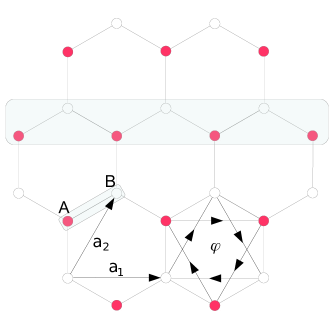
Figure 1: (Color online) Haldane’s model. $A$ (red) and $B$ (white) label sublattice sites, and the boxed pair represents a unit cell. Primitive lattice vectors are chosen to be $\vec{a}_{1}$ and $\vec{a}_{2}$ as shown. Second neighbor hopping between same sublattice sites picks up a phase of $+\phi$ along the arrowed directions and $-\phi$ in opposite directions. Horizontal box encloses a zigzag edge.

In the bulk, the Fourier transformed Hamiltonian is

$$H(\vec{k})=\omega(\vec{k})+\vec{B}(\vec{k})\cdot\vec{\sigma},$$ (2)

$\vec{\sigma}=(\sigma_{x},\sigma_{y},\sigma_{z})$ are the Pauli matrices in the “isospin” degree of freedom, where $A$ and $B$ are isospin up and down, respectively, and

$$B_{x} =-1-\cos k_{1}-\cos k_{2}$$ (3)

$$B_{y} =-\sin k_{1}-\sin k_{2}$$

$$B_{z} =m+2\sin\phi\bigl{[}t_{1}\sin k_{1}-t_{2}\sin k_{2}+t_{3}\sin(k_{2}-k_{1})\bigr{]}$$

$$\omega =-2\cos\phi\bigl{[}t_{1}\cos k_{1}+t_{2}\cos k_{2}+t_{3}\cos(k_{2}-k_{1})\bigr{]}$$

Here, $k_{i}=\vec{k}\cdot\vec{a}_{i}\in[0,2\pi]$ are the Bloch phases along the two primitive vectors. The bulk topology is characterized by the Chern number $C$ of the upper band, which is the winding number of the unit vector ${\hat{B}}({\hat{k}})$ over the Brillouin zone. That is to say, if by varying $(k_{1},k_{2})$ over the first Brillouin zone, $\hat{B}=\vec{B}/|B|$ covers the unit sphere once ($|C|=1$), then the system is in its topological phase, otherwise it is in its trivial phase. Equivalently, in the topological phase the origin is inside the surface swept out by $\vec{B}$, while in the nontopological phase it lies outside. The topological phase transition thus takes place when the origin is crossed by $\vec{B}$ at some $\vec{k}$ points, where the gap $\Delta=2|B|$ will vanish. Following eqn. 3, this can only happen at the graphene Dirac points, $(k_{1},k_{2})=\pm(2\pi/3,-2\pi/3)\equiv\vec{K}_{\pm}$, where $B_{x}=B_{y}=0$. The corresponding $B_{z}$ values necessarily have opposite signs in the topological phase (so that the origin is enclosed), i.e.Haldane (1988),

$$|m|-\sqrt{3}\left|(t_{1}+t_{2}+t_{3})\sin\phi\right|\begin{cases}<0&\text{topological}\\ >0&\text{trivial}\end{cases}.$$ (4)

In the trivial phase, the eigenstates just below the gap at both Dirac points are entirely concentrated on the same sublattice. In the topological phase, however, they are concentrated on opposite sublattices.

II.1 Zigzag edge states

One way of solving the edge spectrum of tight binding models is to use the transfer matrix formalism, following Hatsugai’s investigation Hatsugai (1993) of the Hofstadter problem Hofstadter (1976). It is worthwhile to first think about its application in the Haldane model. In the Hofstadter problem, the system is immersed in a uniform magnetic field with rational flux $2\pi p/q$ per (square, say) plaquette, and the lattice vector potential is periodic on the scale of the magnetic unit cell, which consists of $q$ structural cells. As a result, a $qN$-step transfer matrix $\mathcal{M}_{qN}$ can be broken up into a product of $N$ identical matrices each equal to a $q$-step transfer matrix, $\mathcal{M}_{qN}=(\mathcal{M}_{q})^{N}$, thus the solutions of $\mathcal{M}_{q}$ comprise a special set of the solutions of $\mathcal{M}_{qN}$. Physically this means the edge spectrum of a system with $qN-1$ structural cells in the open direction is identical to the full spectrum of a system with $q-1$ structural cells. Thus numerically, one only needs to diagonalize a $(q-1)\times(q-1)$ Hamiltonian to find the edge spectrum of a $(qN-1)\times(qN-1)$ Hamiltanion. Clearly the method is most efficient in a situation where the transfer matrix has such a decomposition, e.g., a graphene sheet in magnetic field Hatsugai et al. (2006). The Haldane model has no macroscopic magnetic field (an essential virtue of the model), thus the transfer matrix formalism yields little advantage over directly diagonalizing the full Hamiltonian. Still, one may employ it to analyze the Riemann sheet structure of the complex energy, which is studied in Ref. Hao et al., 2008, but that is not our focus here.

A useful feature of Hatsugai’s solution is that it can be written as a direct product of an $N$-component real space part, corresponding to the magnetic unit cell coordinate, and a $q$-component internal space part, corresponding to the lattice points within each magnetic unit cell. (See, e.g., the appendix of Ref. Huang and Arovas, 2012.) This is by no means a general form for edge states. All Bloch states on the other hand have such a decomposition. What we found for the Haldane model is that the edge states in the case of a zigzag edge can also be direct-product-decomposed, with the following caveats. First, while the real space part in the Hofstadter model has exact exponential dependence on the coordinate (equivalent to an imaginary Bloch wavevector), which is due to decomposition of the transfer matrix, this is not so in the Haldane model (nor is this surprising since the macroscopic magnetic field is zero). Second, the boundary condition used in the Hofstadter model corresponds to an open edge. In the Haldane model, the boundary condition must be tuned self-consistently to conform with the direct product Ansatz. Only those boundary conditions with vanishing magnitude will correspond to an edge state at an open boundary, as opposed to, say, an enhanced-tunneling boundary.

We now proceed to solve for the zigzag edge states.

II.1.1 Twisted-boundary Hamiltonian and gauge transformation

The zigzag edge is parallel to $\vec{a}_{1}$ (see the horizontal box in Fig. 1), hence $k_{1}=\vec{k}\cdot\vec{a}_{1}$ is a good quantum number. Assume there are $N$ unit cells in the $\vec{a}_{2}$ direction. At each $k_{1}$, the effective $1$-D system is described by the following Hamiltonian,

$$\mathcal{H}(k_{1})=\sum_{n,n^{\prime}=1}^{N}\Bigl{[}a_{n}^{\dagger}K^{(1)}_{n,n^{\prime}}a^{\vphantom{\dagger}}_{n^{\prime}}+b_{n}^{\dagger}K^{(2)}_{n,n^{\prime}}b^{\vphantom{\dagger}}_{n^{\prime}}\\ +a_{n}^{\dagger}R^{\vphantom{\dagger}}_{n,n^{\prime}}b^{\vphantom{\dagger}}_{n^{\prime}}+b_{n}^{\dagger}R^{\dagger}_{n,n^{\prime}}a^{\vphantom{\dagger}}_{n^{\prime}}\Bigr{]}$$ (5)

Here $a^{\dagger}_{n}$ and $b^{\dagger}_{n}$ are creation operators on the A and B site of the $n^{\rm th}$ unit cell, respectively. The coefficient matrices $K^{(i)}$ connect sites on the same sublattice, and $R$ connects different sublattices. Their nonzero matrix elements are given by

$$K^{(i)} =\begin{pmatrix}h_{i}&v_{i}&&&\tilde{v}_{i}^{*}\\ v_{i}^{*}&h_{i}&v_{i}\\ &\ddots&\ddots&\ddots\\ &&v_{i}^{*}&h_{i}&v_{i}\\ \tilde{v}_{i}&&&v_{i}^{*}&h_{i}\end{pmatrix}\ ,$$ (6)

$$R =\begin{pmatrix}p_{1}&&&&\tilde{v}_{21}^{*}\\ p_{2}&p_{1}\\ &\ddots&\ddots\\ &&p_{2}&p_{1}\\ \tilde{v}_{12}&&&p_{2}&p_{1}\end{pmatrix}\ .$$ (7)

The individual matrix elements can be obtained from Fourier transforming the bulk Hamiltonian eqn. 2,

$$h\equiv\sum_{k_{2}}H(k_{1},k_{2})=\begin{pmatrix}h_{1}&p_{1}\\ p_{1}^{*}&h_{2}\end{pmatrix},$$ (8)

$$v\equiv\sum_{k_{2}}H(k_{1},k_{2})e^{-ik_{2}}=\begin{pmatrix}v_{1}&0\\ p_{2}&v_{2}\end{pmatrix}$$ (9)

with

$$h_{1} =m-2t_{1}\cos(\phi+k_{1})\ ,$$ (10)

$$h_{2} =-m-2t_{1}\cos(\phi-k_{1})\ ,$$ (11)

$$v_{1} =-t_{2}e^{-i\phi}-t_{3}e^{i\phi}e^{-ik_{1}}\ ,$$ (12)

$$v_{2} =-t_{2}e^{i\phi}-t_{3}e^{-i\phi}e^{-ik_{1}}\ ,$$ (13)

$$p_{1} =-1-e^{-ik_{1}}\quad,\quad p_{2}=-1\ .$$ (14)

We note that swapping subscripts $1$ and $2$ on the left hand sides yields a Hamiltonian with the so-called bearded edge. The method we describe below applies to both types of edge.

The following gauge transformation makes both $p_{1}$ and $p_{2}$ real,

$$a_{n}(k_{1}) \rightarrow a_{n}(k_{1})\,e^{-i(n-1)k_{1}/2}\ ,$$

$$b_{n}(k_{1}) \rightarrow b_{n}(k_{1})\,e^{-ink_{1}/2}\ ,$$ (15)

by which $v_{i}\rightarrow v_{i}\,e^{ik_{1}/2}$ and $p_{1}\rightarrow p_{1}\,e^{ik_{1}/2}$, viz.,

$$v_{1}\rightarrow-(t_{2}+t_{3})\cos(\phi-{\textstyle{k_{1}\over 2}})+i(t_{2}-t_{3})\sin(\phi-{\textstyle{k_{1}\over 2}}),$$

$$v_{2}\rightarrow-(t_{2}+t_{3})\cos(\phi+{\textstyle{k_{1}\over 2}})-i(t_{2}-t_{3})\sin(\phi+{\textstyle{k_{1}\over 2}}),$$

$$p_{1}\rightarrow-2\cos{\textstyle{k_{1}\over 2}}.$$ (16)

In eqns. 6 and 7, a twisted boundary condition Qi et al. (2006) is used:

$$\tilde{v}\equiv\rho\,Uv=\begin{pmatrix}\tilde{v}_{1}&\tilde{v}_{12}\\ \tilde{v}_{21}&\tilde{v}_{2}\end{pmatrix}.$$ (17)

$\rho$ is a real number controlling the “tunnelling strength” between the two edges, and $U$ is a unitary $2\times 2$ matrix that describes an “isospin-dependent” phase twisting over the boundary. For an open boundary, $\rho\rightarrow 0$. For periodic boundary conditions, $\rho=1$ with $U=\mathbb{I}$ (without the gauge transformation of eqn. II.1.1) or $U=e^{-iNk_{1}/2}\,\mathbb{I}$ (with eqn. II.1.1), where $\mathbb{I}$ is the $2\times 2$ identity matrix. Introducing twisted boundary condition may seem to overcomplicate the situation, but as we shall see it allows us to make progress toward an analytical solution.

The eigenvalue problem can now be written as

$$K^{(1)}|\psi_{A}\rangle+R\,|\psi_{B}\rangle=\varepsilon\,|\psi_{A}\rangle\ ,$$

$$K^{(2)}|\psi_{B}\rangle+R^{\dagger}\,|\psi_{A}\rangle=\varepsilon\,|\psi_{B}\rangle\ ,$$ (18)

where $|\psi_{A}\rangle$ and $|\psi_{B}\rangle$ are the “wavefunctions” of the $A$ and $B$ sublattices, both of which are $N$-dimensional column vectors.

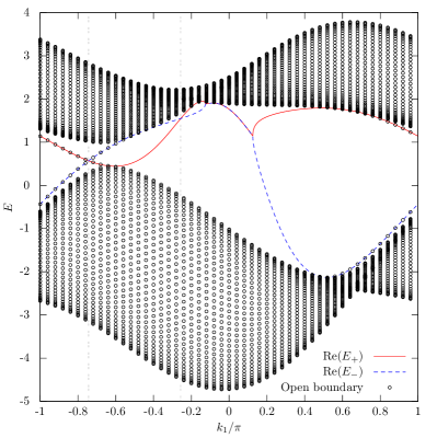
(a)  Ansatz vs. open boundary spectrum

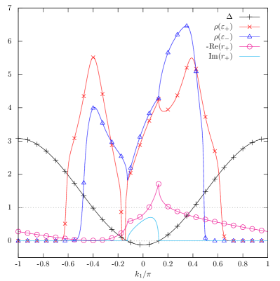
(b)  auxiliary quantities

Figure 2: (Color online) Zigzag edge modes for $[t_{1},t_{2},t_{3}]=[0.3,0.4,0.5]$, $m=1.4$, $\phi=0.3\pi$, $N=40$. (a) Circular dots are obtained from diagonalizing an open boundary Hamiltonian, eqn. 5 with $\rho=0$. Colored curves are Ansatz solutions, eqn. 24. Gray vertical lines mark the edge level crossing points given by eqn. 30. (b) Auxiliary quantities. $\Delta$ is the discriminant in eqn. 27, only $\Delta>0$ yields real solutions of edge energy $\varepsilon_{\pm}$ and is physical. $r_{+}$: the ratio of eqn. 21 corresponding to the $\varepsilon_{+}$ branch. It is real if $\Delta>0$. $r_{-}$ can be obtained from eqn. 96 and is not plotted here. $\rho(\varepsilon_{\pm})$: the inter-edge tunnelling strength as defined in eqn. 5. These are solved in a self-consist fashion in Appendix A. $\rho\rightarrow 0$ for open boundary, $\rho>1$ for “enhanced-tunnelling” boundary. The transition $\rho=1$ corresponds to bulk modes.

II.1.2 Edge state Ansatz and energy

We look for solutions of the form $|\psi_{A}\rangle=|\psi\rangle$ and $|\psi_{B}\rangle=\lambda|\psi\rangle$. In terms of the direct-product decomposition discussed earlier, $|\psi\rangle$ is the real space part and $\left(\begin{smallmatrix}1\\ \lambda\end{smallmatrix}\right)$ is the internal space part. Eqn. 18 now becomes

$$(K^{(1)}+\lambda R-\varepsilon)|\psi\rangle=0\ ,$$ (19)

$$(\lambda K^{(2)}+R^{\dagger}-\lambda\varepsilon)|\psi\rangle=0\ .$$ (20)

A sufficient condition for both equations to be satisfied is that the coefficient matrices are proportional element by element,

$${h_{1}+\lambda p_{1}-\varepsilon\over h_{2}+\lambda^{-1}p_{1}-\varepsilon}={v_{1}\over v_{2}+\lambda^{-1}p_{2}}={v_{1}^{*}+\lambda p_{2}\over v_{2}^{*}}\equiv r\ .$$ (21)

This gives, at each value of $k_{1}$, two equations (the ratio $r$ itself being yet undetermined) for the two unknowns $\lambda$ and $\varepsilon$. The solutions are

$$\lambda_{\pm}={v_{1}v_{2}^{*}-v_{2}v_{1}^{*}-p_{2}^{2}\pm\sqrt{d^{2}-4|v_{1}v_{2}|^{2}}\over 2p_{2}v_{2}}\ ,$$ (22)

$$r_{\pm}\equiv r(\lambda_{\pm})={d\pm\sqrt{d^{2}-4|v_{1}v_{2}|^{2}}\over 2|v_{2}|^{2}}\ ,$$ (23)

$$\varepsilon_{\pm}={r_{\pm}(p_{2}h_{2}-2p_{1}\textsf{Re}\,v_{2})-(p_{2}h_{1}-2p_{1}\textsf{Re}\,v_{1})\over p_{2}(r_{\pm}-1)}\ ,$$ (24)

where Re indicates the real part, $\pm$ denotes the branch of solution, and

$$d=v_{1}v_{2}^{*}+v_{2}v_{1}^{*}-p_{2}^{2}\in\mathbb{R}\ .$$ (25)

See Appendix  A for details regarding derivation.

Eqn. 23 becomes singular when $v_{2}=0$, which could happen for the zigzag edge if $t_{2}=t_{3}$ and $k_{1}=\pi-2\phi$. For this particular parameter set, one can readily verify, by Taylor expansion in $v_{2}$, that

$$\lambda_{+}=v_{1}\ ,\quad r_{+}=-v_{1}^{2}\ ,\quad\varepsilon_{+}={h_{2}v_{1}^{2}+2p_{1}v_{1}+h_{1}\over 1+v_{1}^{2}}\ ,$$

$$\lambda_{-}^{-1}=v_{2}\rightarrow 0\ ,\quad r_{-}^{-1}=-v_{2}^{2}\rightarrow 0\ ,\quad\varepsilon_{-}=h_{2}\ .$$ (26)

These results also hold both for graphene ($m=0$) and for boron nitride ($m\neq 0$). In both cases, second neighbor hoppings are turned off, rendering $v_{1}=v_{2}=0$. Clearly, $\lambda_{+}=r_{+}=\lambda_{-}^{-1}=r_{-}^{-1}=0$, and $\varepsilon_{\pm}=\pm m$. As will be shown in Appendix A, $\rho\rightarrow 0$ if $|k_{1}|>2\pi/3$, so solutions there correspond to edge modes with open boundary.

A natural question arises regarding the reality of the energy eqn. 24. As long as we can find wavefunctions complying with the Ansatz $|\psi_{B}\rangle=\lambda\,|\psi_{A}\rangle$, $\varepsilon_{\pm}$ will be eigenvalues of a Hermitian matrix, and hence real. This implies that $r_{\pm}$ are also real (cf. eqn. 98). Thus by eqn. 23, our Ansatz yields real solutions, with some choice of $\rho\,U$, provided the discriminant satisfies

$$\Delta=d^{2}-4|v_{1}v_{2}|^{2}\geq 0\ .$$ (27)

Note that this condition is valid for all $k_{1}$.

Although real solutions exist for all $k_{1}$ with $\Delta(k_{1})\geq 0$, they do not necessarily correspond to open boundaries. Normally, wavefunctions are solved after fixing boundary conditions ($\rho$ and $U$), but here, we enforced a particular form of solution, which will not be consistent with arbitrary $\rho\,U$. Instead, the matrix $\rho\,U$ is to be determined self-consistently from the Ansatz, and is in general $k_{1}$-dependent. This is discussed in detail in Appendix A. For now, we just note that only when $\rho\rightarrow 0$ will the solution be valid for open boundary. Clearly, as $\rho$ varies with $k_{1}$, the transition from an open boundary solution to that of an “enhanced tunnelling” boundary will happen when $\rho=1$, at which point the edge solution merges into the bulk ($|\psi\rangle$ becomes extended instead of localized).

Fig. 2 shows the Ansatz solutions (colored curves) comparing with the open boundary spectrum (circular dots) in 2(a), and auxiliary variables $\Delta$, $r(\varepsilon_{+})$ and $\rho(\varepsilon_{\pm})$ in 2(b). Parameters are chosen to exhibit most of the possible scenarios, $[t_{1},t_{2},t_{3}]=[0.3,0.4,0.5]$, $m=1.4$, $\phi=0.3\pi$, $N=40$:
(1) $\Delta<0$ for $|k_{1}|\lesssim 0.125$. In this region the Ansatz does not yield real energy solutions.
(2) For $|k_{1}|\gtrsim 0.125$, the Ansatz yields physical solutions. One then computes $\rho$ self-consistently; $\rho\ll 1$ means open boundary, whereas $\rho>1$ means enhanced-tunneling boundary. The transition happens when the open boundary edge modes merge with the bulk bands. The $\varepsilon_{+}$ branch (red curve) has open boundary for $k_{1}\in[-\pi,-0.62\pi]\cup[-0.17\pi,-0.14\pi]\cup[0.62\pi,\pi]$, while the $\varepsilon_{-}$ branch (blue curve) has open boundary for $k_{1}\in[-\pi,-0.48\pi]\cup[0.49\pi,\pi]$. In these regions, the Ansatz solutions overlap with the open-boundary numerics (filled circles). Note that the $\varepsilon_{+}$ branch briefly becomes open boundary in $[-0.17\pi,-0.14\pi]$. Without the Ansatz solution, one would have taken it to be part of the bulk spectrum.
(3) Within the physical regime ($\Delta>0$), the two branches cross twice, marked by the two vertical gray lines, one with $\rho(\varepsilon_{\pm})\rightarrow 0$ and the other with $\rho(\varepsilon_{\pm})>1$. In both cases $\rho(\varepsilon_{+})=\rho(\varepsilon_{-})$. These two edge crossing $k_{1}$ points are described by eqn. 30 which will be discussed in the next section. While only the one with $\rho\rightarrow 0$ is relevant for the open-boundary edge spectrum, we shall see in the next section that both have geometrical significance and will be reflected in the entanglement spectrum and Berry phase flow.

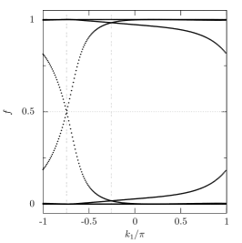
(a)  Periodic-boundary entanglement occupancy

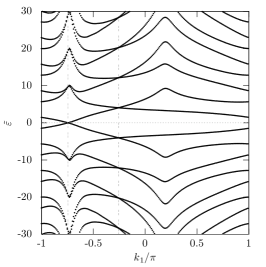
(b)  Periodic-boundary entanglement quasi-energy

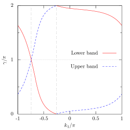
(c)  Deviation of Wannier centers from unit cell boundary

Figure 3: (Color online) Coincidence of level crossings in entanglement and Berry phase flows. (a): Entanglement occupancy. (b): Entanglement quasienergy. (c): Deviations of Wannier centers from their corresponding unit cell boundary; mathematically this is the Berry phase; plotted for both the occupied and unoccupied bands. Periodic boundary conditions are used. Parameters used here are the same as in Fig. 2: $[t_{1},t_{2},t_{3}]=[0.3,0.4,0.5]$, $m=1.4$, $\phi=0.3\pi$. Entanglement spectra are computed for the lower half system with $M=N/2=20$ unit cells in the $\vec{a}_{2}$ direction, where $N=40$ is the number of unit cells of the full system, and Fermi energy is placed in the gap, $E_{\textsf{F}}=0.6$. Berry phases are computed using $100$ steps in the $k_{2}$ integration. Notice the similarity between the entanglement occupancy and the Berry phases. This is due to the former being a coarse-grained version of the latter in the sense of Ref. Huang and Arovas, 2012. Notice that in all three plots, level crossings occur at the same $k_{\rm c}$ points given by eqn. 30. Although the open boundary edge modes only cross at one of the two $k_{\rm c}$, the entanglement spectra and the Berry phases cross at both $k_{\rm c}$, but with different $f$, $\tilde{\varepsilon}$ and $\gamma$ values. $f={\textstyle{1\over 2}}$, $\tilde{\varepsilon}=0$ and $\gamma=\pi$ at the open-boundary edge crossing point. At the other $k_{\rm c}$ point, $\gamma=0$. Notice also that in the quasienergy plot, level crossings are not restricted to the central two levels but extend all the way to big $|\gamma|$ values, and are pinned at the same $k_{\rm c}$ values.

II.2 Topological signatures in edge, entanglement and Wannier spectra

A gapless edge spectral flow is one of the most conspicuous real-space manifestation of nontrivial topology of band insulators. But as discussed in the introduction, it sometimes fails to reveal every topological difference a band insulator can have from its atomic limit Hughes et al. (2011), which the entanglement spectrum can capture. In the non-interacting fermion case, the entanglement occupancy spectrum is the eigenvalues of a submatrix $G$ of the one-body ground state projector $\mathcal{G}$ Cheong and Henley (2004); Peschel (2003), with the dimension of $G$ given by the entanglement cut. The eigenvalues of $\mathcal{G}$ itself are just $0$s and $1$s, but for a system with nontrivial topology, the eigenvalues of $G$ exhibit a spectral flow from $0$ to $1$, as a function of the momentum $\vec{k}^{\vphantom{\dagger}}_{\perp}$ along the entanglement cut. The reason why the entanglement cut would induce such a flow can be understood intuitively in terms of the Wannier states. One can always recombine the Bloch states that constitute $\mathcal{G}$ (assuming the system is periodic) into a set of spatially localized Wannier states. If a Wannier state resides in either half of the partition, it has almost perfect projection onto that half, and the corresponding entanglement occupancy is very near $0$ or $1$. If on the other hand the entanglement cut passes right through a Wannier state (the exact meaning of which we shall discuss in §II.2.3), then it has significant projection onto both halves, correspondingly the entanglement occupancy is near ${\textstyle{1\over 2}}$. In the topological phase, the Wannier states themselves flow with respect to $\vec{k}^{\vphantom{\dagger}}_{\perp}$ Qi (2011); Soluyanov and Vanderbilt (2011); Yu et al. (2011), thus when one such state passes through the entanglement cut, a corresponding entanglement flow arises. One can see that the position of the Wannier states, or the Wannier spectrum, is closely related to the entanglement spectrum, and that a nontrivial topology underlies the $f={\textstyle{1\over 2}}$ entanglement occupancy mode, and a half-odd-integer Wannier center. It is thus interesting to note that in the Haldane model, the edge crossing point, the half occupancy mode and the half-odd-integer Wannier center all coincide at the same $k_{1}$ point. See Fig. 3. In this section we shall study the reason underlying this coincidence. We mention that there are several other works Thonhauser and Vanderbilt (2006); Coh and Vanderbilt (2009) studying the charge polarization of the Haldane model, from the Wannier function perspective.

II.2.1 Edge modes crossing points

With the edge solution in §II.1, we can identify the exact location of these crossing points. The condition for $\varepsilon_{+}=\varepsilon_{-}$ is that

$$p_{2}(h_{1}-h_{2})+2p_{1}\textsf{Re}(v_{2}-v_{1})=0\;,$$ (28)

see Appendix A for derivation. For the zigzag edge, this implies

$$m+2\sin\phi\sin k_{\rm c}(t_{1}+t_{2}+t_{3})=0$$ (29)

whence

$$k_{\rm c}=\begin{cases}-\sin^{-1}\dfrac{m}{2(t_{1}+t_{2}+t_{3})\sin\phi}\\ \quad&\text{ or }\\ \pi+\sin^{-1}\dfrac{m}{2(t_{1}+t_{2}+t_{3})\sin\phi}\end{cases}$$ (30)

Here $k_{\rm c}$ denotes the values of $k_{1}$ where the two edge modes are energetically degenerate. The bearded edge solution is obtained by switching the $1$ and $2$ suffixes in $p_{i},h_{i}$ and $v_{i}$, for which eqn. 28 implies

$$(m+2t_{1}\sin\phi\sin k_{\rm c})\cos{\textstyle{k_{\rm c}\over 2}}\\ +(t_{2}+t_{3})\sin\phi\sin{\textstyle{k_{\rm c}\over 2}}=0.$$ (31)

This could be recast as a cubic equation for $\tan(k_{\rm c}/2)$, but this does not afford a particularly simple closed form solution.

One can see from Fig. 2 that only one of the two $k_{\rm c}$ has $\rho\rightarrow 0$ and corresponds to an open boundary edge mode. The other one is of an enhanced-tunnelling boundary; in some parameter settings it even lies in the region $\Delta<0$ where the Ansatz solution is complex. However, the enhanced-tunnelling $k_{\rm c}$ is still special in the entanglement and Wannier center flows, as can be seen in Fig. 3. What is the significance about these edge crossing points? Recall that the bulk Hamiltonian $H(k_{1},k_{2})$ maps each $\vec{k}$ to a $\vec{B}(\vec{k})$ vector. Fixing $k_{1}$ while varying $k_{2}$ will drive the $\vec{B}$ vector along a closed curve in $3$D. It turns out that at both $k_{\rm c}$, this curve lies on a plane passing through the origin. To see this, we note that at the edge crossing point, the $2\times 2$ blocks $h(k_{1})$ and $v(k_{1})$ are related via

$$h=\varepsilon_{\rm c}\,\mathbb{I}+{p_{1}\over p_{2}}\left(v+v^{\dagger}\right)$$ (32)

where $\varepsilon_{\rm c}=\varepsilon_{+}(k_{\rm c})=\varepsilon_{-}(k_{\rm c})$ (cf. eqn. 101). The bulk Hamiltonian at the edge crossing points is then

$$H(k_{\rm c},k_{2}) =h+v\,e^{ik_{2}}+v^{\dagger}\,e^{-ik_{2}}$$

$$=\left[v\left({p_{1}\over p_{2}}+e^{ik_{2}}\right)+{\rm H.c.}\right]+\varepsilon_{\rm c}\,\mathbb{I},$$ (33)

and the corresponding $\vec{B}(k_{\rm c},k_{2})$ is

$$B_{z}=\left({p_{1}\over p_{2}}+\cos k_{2}\right)\textsf{Re}\,(v_{1}-v_{2})-\sin k_{2}\,\textsf{Im}\,(v_{1}-v_{2})\;,$$

$$B_{x}=p_{1}+p_{2}\cos k_{2}\;,\quad B_{y}=p_{2}\sin k_{2}\;,$$ (34)

note in particular that all components are independent of $m$, which is the term that breaks the inversion of the two sublattices. It is then easy to check that

$$\vec{B}(k_{\rm c},k_{2})=B_{x}\left(\hat{x}-\textsf{Re}(q)\>\hat{z}\right)+B_{y}\left(\hat{y}-\textsf{Im}(q)\>\hat{z}\right)$$ (35)

where

$$q={v_{2}-v_{1}\over p_{2}}$$ (36)

is independent of $k_{2}$. The path of $\vec{B}(k_{\rm c},k_{2})$ is thus coplanar and normal to the vector

$$\vec{n}\equiv\textsf{Re}(q)\>\hat{x}+\textsf{Im}(q)\>\hat{y}+\hat{z}.$$ (37)

An unrestricted $(B_{x},B_{y})$ pair can describe any point on the plane. Clearly the origin itself is on the plane. The actual path of $\vec{B}(k_{\rm c},k_{2})$ is restricted to those allowed by eqn. 34.

An interesting observation is that in graphene, the bulk $2\times 2$ Hamiltonian is always off-diagonal, thus it is coplanar at any $k_{1}$ value. The origin is inside the path of $\vec{B}$ for $|k_{1}|>2\pi/3$, and outside otherwise, hence the well known result that its two zigzag edge modes are degenerate at $\varepsilon=0$ for $|k_{1}|>2\pi/3$. For the bearded edge, the degenerate edge modes connect the two Dirac points in the other way, namely with $|k_{1}|<2\pi/3$.

II.2.2 Integer and half-odd-integer Wannier centers

For a general one-dimensional periodic system, or higher-dimensional system with $\vec{k}^{\vphantom{\dagger}}_{\perp}$ specified, the Wannier centers can be defined as the nonvanishing eigenvalues of the band-projected real-space operator

$$\mathcal{G}(\vec{k}^{\vphantom{\dagger}}_{\perp})\,R\>\mathcal{G}(\vec{k}^{\vphantom{\dagger}}_{\perp})$$ (38)

where $\mathcal{G}(\vec{k}^{\vphantom{\dagger}}_{\perp})$ is the filled band projector (or sum of projectors for multiple bands) at $\vec{k}^{\vphantom{\dagger}}_{\perp}$, $R=\hat{Y}\!\otimes\!\mathbb{I}$ in which $\hat{Y}=\textsf{diag}(1,2,\ldots,N)$ measures real space (i.e., unit cell) coordinates, $N$ being the number of unit cells in the longitudinal direction, and $\mathbb{I}$ is the $q\times q$ unity acting on the $q$-dimensional internal space. The corresponding eigenstates are defined as the Wannier states Kivelson (1982). The monolayer Haldane model has only one band occupied at half filling. When $\mathcal{G}$ contains only one band, the eigenvalues of eqn. 38 are Qi (2011)

$$\lambda_{I}(\vec{k}^{\vphantom{\dagger}}_{\perp})={\gamma(\vec{k}^{\vphantom{\dagger}}_{\perp})\over 2\pi}+I\quad,\quad I=1,2,\ldots N$$ (39)

where $I$ labels the unit cell, and $\gamma(\vec{k}^{\vphantom{\dagger}}_{\perp})$ is the Berry phase of the band,

$$\gamma(\vec{k}^{\vphantom{\dagger}}_{\perp})=\int\limits_{0}^{2\pi}\!\!dk^{\vphantom{\dagger}}_{\parallel}A(k^{\vphantom{\dagger}}_{\parallel})\quad,\quad A(k^{\vphantom{\dagger}}_{\parallel})\equiv i\,\langle\psi|\,\partial_{k^{\vphantom{\dagger}}_{\parallel}}\,|\psi\rangle\;.$$ (40)

The $\vec{k}^{\vphantom{\dagger}}_{\perp}$ dependence of $A$ is suppressed. $A$ is the $k^{\vphantom{\dagger}}_{\parallel}$ component of the Berry connection vector at fixed $\vec{k}^{\vphantom{\dagger}}_{\perp}$. Thus the offset of the Wannier centers from the unit cell boundaries are uniform and are given by the Berry phaseZak (1989).

In the Haldane model, $\vec{k}^{\vphantom{\dagger}}_{\perp}=k_{1}$ and $k^{\vphantom{\dagger}}_{\parallel}=k_{2}$. The lower band projector is

$$\mathcal{G}(k_{1})=\sum_{k_{2}}|\Psi(\vec{k})\rangle\langle\Psi(\vec{k})|\;,$$ (41)

$$|\Psi(\vec{k})\rangle\equiv|k_{2}\rangle\otimes|\psi(k_{1},k_{2})\rangle\;,$$ (42)

where the internal part $|\psi(k_{1},k_{2})\rangle$ is the lower band eigenstate of the bulk Hamiltonian eqn. 2, and the real-space part $|k_{2}\rangle$ is the Bloch wave in the $\vec{a}_{2}$ direction, $\langle y|k_{2}\rangle=e^{ik_{2}y}/\sqrt{N}$. The upper band projector is similarly defined. We plot the Berry phase in Fig. 3(c), where the red and blue curve correspond to the lower and upper band, respectively. We will show below that coplanarity of $\vec{B}$ at $k_{\rm c}$ fixes the Berry phases there to be either $\pi$ or $0$, depending on whether or not the origin lies inside the path of $\vec{B}$. In fact, this holds for any two-band model with coplanar $k$ points. Recall $H(\vec{k})=\omega(\vec{k})\mathbb{I}+\vec{B}(\vec{k})\cdot\vec{\sigma}$. Let $\left(B(\vec{k}),\vartheta(\vec{k}),\varphi(\vec{k})\right)$ be the spherical coordinate of $\vec{B}(\vec{k})$, then the lower band eigenstate is

$$|\psi\rangle=\begin{pmatrix}-\sin{\textstyle{\vartheta\over 2}}\\ e^{i\varphi}\cos{\textstyle{\vartheta\over 2}}\end{pmatrix}\;,$$ (43)

whence

$$A(k_{2})=-{\textstyle{1\over 2}}(1+\cos\vartheta){\partial\varphi\over\partial k_{2}}$$ (44)

and

$$\gamma(k_{1})=-{\textstyle{1\over 2}}\!\!\!\!\int\limits_{\varphi(0)}^{\varphi(2\pi)}\!\!\!\!\!d\varphi\,(1+\cos\vartheta)\;,$$ (45)

where $\varphi(0)=\varphi(k_{1},k_{2}=0)$ and $\varphi(2\pi)=\varphi(k_{1},k_{2}=2\pi)$. At the edge crossing $k_{1}$, $\hat{B}$ is comprised of points on a great circle (since the origin is on the plane), so one can always rotate the internal space to a frame where the plane normal $\vec{n}$ (eqn. 37) coincides with the $\hat{z}$ axis, then $\cos\vartheta=0$ everywhere on the coplanar path which is now lying in the new $xy$ plane. The Berry phases at coplanar $k_{1}$ points are simply $2\pi$ times half the (negative) winding number $w$ of the path of $\vec{B}$,

$$\gamma(k_{\rm c})=-w\pi\quad,\quad w\equiv{\varphi(2\pi)-\varphi(0)\over 2\pi}\;.$$ (46)

Note that this rotation amounts to applying the following unitary transformation to the band projector $\mathcal{G}$ in eqn. 38,

$$\mathcal{G}\rightarrow\tilde{\mathcal{G}}=U\mathcal{G}\,U^{\dagger}\quad,\quad U=\mathbb{I}\otimes D(\hat{n})$$ (47)

where $D(\hat{n})$ is the aforementioned internal space rotation that depends only on $\hat{n}$. Since $UR\,U^{\dagger}=R$, both $\mathcal{G}R\,\mathcal{G}$ and $\tilde{\mathcal{G}}R\,\tilde{\mathcal{G}}$ have the same spectrum, so the resulting Wannier centers and Berry phases are independent of whether $\mathcal{G}$ or $\tilde{\mathcal{G}}$ is used.

For the Haldane model, the topological phase has Chern number $|C|=1$, so the winding number at any $k_{1}$ is at most $|w|=1$, hence $\gamma(k_{\rm c})$ is either $\pm\pi$ (origin inside) or $0$ (origin outside), which is what we see in Fig. 3(c). In the non-topological phase, $\gamma$ at both $k_{\rm c}$ will be $0$.

II.2.3 Entanglement Half Occupancy Mode

As discussed in the introduction, the entanglement spectrum can be associated with a coarse-graining of the Wannier centers. By coarse-graining, we mean replacing the real-space operator $R=\hat{Y}\otimes 1$ with the projector

$$P_{M}=f(\hat{Y},M)\otimes 1\;,$$ (48)

$$f(y,M)=\begin{cases}1&\text{if }y<M+{\textstyle{1\over 2}}\\ 0&\text{if }y>M+{\textstyle{1\over 2}}\ ,\end{cases}$$ (49)

where $M$ is an integer. In so doing, all Wannier center flows except those between unit cells $M$ and $M+1$ are suppressed. Since $\mathcal{G}$ and $P_{M}$ are both projectors, $\mathcal{G}P_{M}\mathcal{G}$ and $P_{M}\mathcal{G}P_{M}$ share the same spectrum (cf. Appendix D). The latter is nothing but the restricted correlation matrix whose eigenvalues are the entanglement occupancy spectrum, and the integer $M$ corresponds to the entanglement cut. The entanglement eigenstates, $|\tilde{\Psi}\rangle$, are projections of eigenstates $|\Psi\rangle$ of $\mathcal{G}P_{M}\mathcal{G}$ onto the half space $y\leq M$ by $P_{M}$, i.e. $|\tilde{\Psi}\rangle=P_{M}|\Psi\rangle$.

We found that at the edge crossing point $k_{\rm c}$, in the case of odd winding number, the periodic boundary entanglement occupancy spectrum has two modes intersecting at $f={\textstyle{1\over 2}}$ (Fig. 3(a)), which corresponds to a zero entanglement quasi-energy (Fig. 3(b)). It is evident from Fig. 3(b) that the entanglement quasi-energy spectrum has a particle-hole symmetry for all $k_{1}$. This is a consequence of the periodic boundary condition: there are two independent flows in Figs. 3(a) and 3(b) – one upward, one downward – because by using periodic boundary condition, an entanglement cut creates two new boundaries in each of the half systems. These two flows intersect at both $k_{\rm c}$ points. Had we started with a $\mathcal{G}$ for an open boundary system (in the $\vec{a}_{2}$ direction), then the entanglement cut would only create one new boundary to each of the half systems, and as a result, in each half system, only one of the two flows, which corresponds to the edge created by the entanglement cut, would survive. In that case, there would be no particle-hole symmetry in the entanglement quasi-energy spectrum for arbitrary $k_{1}$, but only at the edge crossing $k_{\rm c}$ points, where the entanglement spectrum still exhibits particle-hole symmetry, since switching the $\vec{a}_{2}$ boundary condition from periodic to open merely removes the double degeneracy at these points.

In fact, one can argue that in an open boundary system, the $f={\textstyle{1\over 2}}$ level is a consequence of this survival of entanglement particle-hole symmetry at the edge crossing point. Assume the number of unit cells in the full system is $N$ and $N$ is even. In an open boundary system, there are two edge levels, thus each bulk band has $N-1$ bulk levels. At the edge crossing point, both edge levels are either below or above the Fermi energy, so the rank of $\mathcal{G}$ is $N\pm 1$ which is always odd. We may always pick the one half of the bipartite whose size $M\geq\text{rank}(\mathcal{G})$, so that $\text{rank}(G)=\text{rank}(\mathcal{G})$. Thus with the entanglement particle-hole symmetry at the $k_{\rm c}$ point, there must be an odd number of entanglement levels fixed at $f={\textstyle{1\over 2}}$.

With a periodic boundary, the half occupancy modes will appear in the thermodynamic limit, and for small $N$, there is avoided crossing between the two flows. However, the degeneracy is exact for arbitrary even $N$ and $M=N/2$ when $t_{2}=t_{3}$. We prove this in Appendix B. Below, we wish to discuss it following the coarse-graining perspective.

The effect of inserting $R$ and $P_{M}$ in between two band projectors $\mathcal{G}$ is to resolve, in real space, the Bloch states that constitute $\mathcal{G}$. As a result, both the Wannier states and the entanglement states are spatially localized. In this respect, there exists a family of such real-space resolvers $R_{\beta}$, parameterized by an “inverse temperature” $\beta$, that smoothly interpolates between the Wannier and entanglement limits,

$$f_{\beta}(\hat{Y})\equiv{\tanh\left[{\textstyle{1\over 2}}\beta\left(\hat{Y}-{\textstyle{1\over 2}}(N+1)\right)\right]\over\tanh\left[{\textstyle{1\over 4}}\beta(N-1)\right]}\;,$$ (50)

$$R_{\beta}\equiv{\textstyle{1\over 2}}\!\left[(N-1)f_{\beta}(\hat{Y})+N+1\right]\otimes\mathbb{I}\;.$$ (51)

Here, $f_{\beta}$ is obtained by rescaling and shifting the Fermi distribution. The extremal cases are

$$R_{\beta\rightarrow 0}=\hat{Y}\;,$$ (52)

$${R_{\beta\rightarrow\infty}-\mathbb{I}\over N-1}=\mathbb{I}-P_{N/2}\;,$$ (53)

where $\mathbb{I}-P_{N/2}$ is a real space projector onto the $y>N/2$ half. Thus by varying $\beta$, the spectrum $\{r_{a}\}$ of $\mathcal{G}R_{\beta}\,\mathcal{G}$ morphs from the Wannier center spectrum to the entanglement spectrum, providing a one-to-one mapping between the Wannier states and the entanglement states.

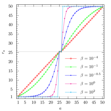
Figure 4: (Color online) Interpolation between Wannier spectrum (red) and entanglement spectrum (light blue) at the edge crossing point $k_{\rm c}$ with winding number $w=1$. $N=50$ unit cells in the $\vec{a}_{2}$ direction, with periodic boundary condition, is used. Other parameters are the same as those used in previous figures: $[t_{1},t_{2},t_{3}]=[0.3,0.4,0.5]$, $m=1.4$, $\phi=0.3\pi$. $\{r_{a}\}$ is the spectrum of $\mathcal{G}R_{\beta}\,\mathcal{G}$, where $a$ is the level index. Different lines correspond to different values of $\beta$. The red dots ($\beta\rightarrow 0$) correspond to the limit of Wannier center spectrum, therefore the vertical coordinates are pinned at half integers (recall the Berry phase is $\pi$). The light blue dots ($\beta\rightarrow\infty$) correspond to the entanglement spectrum (rescaled and shifted according to eqn. 53), by which the mid gap levels at $r_{a}=25.5$ translate to an occupancy of $f=0.5$, $r_{a}=1$ to $f=0$ and $r_{a}=50$ to $f=1$. All curves exhibit particle-hole symmetry (with respect to $r_{a}=25.5$) due to the coplanarity of $\vec{B}$ at $k_{\rm c}$. Notice the two levels pinned at $r_{a}=25.5$ for all $\beta$. Had we used open boundary condition in obtaining $\mathcal{G}$, there would be only one such level.

At the coplanar point $k_{\rm c}$ with winding number $w=1$, two $r_{a}$ levels are pinned at $(N+1)/2$ regardless of the value of $\beta$. This is shown in Fig. 4. The $\beta$-independence suggests a unifying physical origin underlying these levels. We have shown before that, mathematically, the reason for the Wannier spectrum ($\beta\rightarrow 0$) to exhibit such levels is because the Berry phase of the occupied band, which corresponds to the uniform deviation of all Wannier centers from the integers labeling their unit cells, is precisely $\pi$ at the $w=1$ coplanar point. It is instructive to reflect on the physical implication of this result. For convenience, let us rotate to the internal basis where the path of $\vec{B}$ lies in the $xy$ plane, cf. discussion leading to eqn. 46. The Berry connection and its cumulation along the $\vec{B}$ path are thus

$$A(k_{2})=-{1\over 2}\,{\partial\varphi\over\partial k_{2}},\ \int\limits_{0}^{k_{2}}\!\!dk\>A(k)=-{\textstyle{1\over 2}}\left(\bar{\varphi}(k_{2})+wk_{2}\right)$$ (54)

where $\bar{\varphi}(k_{2})\equiv\varphi(k_{2})-wk_{2}$ is the non-winding deviation of $\varphi(k_{2})$ from a pure winding term. The Wannier state corresponding to the $I^{\rm th}$ unit cell is a linear combination of the Bloch states belonging to the occupied band,

$$|\Phi_{I}\rangle=\sum_{k_{2}}f^{(I)}_{k_{2}}\,|\Psi(k_{2})\rangle\quad,\quad I=1,2,\ldots,N$$ (55)

where $|\Psi(k_{2})\rangle$ is the Bloch state defined in eqn. 42, and the coefficients $f$ are Qi (2011)

$$f^{(I)}_{k}={\textstyle{1\over\sqrt{N}}}\exp\left(-iIk-{\textstyle{i\over 2}}\,\bar{\varphi}(k)\right)\;.$$ (56)

Recall that in the rotated frame, the internal-space Bloch states of the occupied band are $|\psi(k_{2})\rangle={\textstyle{1\over\sqrt{2}}}\left(\begin{smallmatrix}-1\\ e^{i\varphi}\end{smallmatrix}\right)$, thus the Wannier wavefunction of the rotated $A$ and $B$ “sublattices” – which are linear combinations of the original $A$ and $B$ sublattices in the same unit cell – are

$$|\Phi_{I}^{(A)}\rangle=-{\textstyle{1\over\sqrt{2}}}\sum_{k_{2}}f^{(I)}_{k_{2}}\,|k_{2}\rangle=-{\textstyle{1\over\sqrt{2}}}\hat{S}^{\dagger}(\bar{\varphi})\,|I\rangle\;,$$ (57)

$$|\Phi_{I}^{(B)}\rangle={\textstyle{1\over\sqrt{2}}}\sum_{k_{2}}e^{i\varphi(k_{2})}f^{(I)}_{k_{2}}\,|k_{2}\rangle={\textstyle{1\over\sqrt{2}}}\hat{S}(\bar{\varphi})\,|I-w\rangle\;.$$ (58)

Here, $|I\rangle=e^{-iIk_{2}}|k_{2}\rangle/\sqrt{N}$ is the $I^{\rm th}$ real-space basis vector; the unitary profile operator $\hat{S}(\bar{\varphi})$ is

$$\hat{S}(\bar{\varphi})\equiv\sum_{k_{2}}|k_{2}\rangle\exp\left({\textstyle{i\over 2}}\bar{\varphi}(k_{2})\right)\langle k_{2}|$$ (59)

and its effect on $|I\rangle$ is to generate a wavepacket centered at the $I$, with its profile determined by the details of the fluctuation $\bar{\varphi}(k)$. We can then conclude that at the coplanar $k_{\rm c}$ points, the two sublattices of the Wannier states (in the rotated frame) are localized in different unit cells with a separation given by the winding number $w$ of the path of $\vec{B}$. The Wannier centers are spatial averages of the locations of the two sublattice wavefunctions, $\lambda_{I}=I-w/2$, thus for odd $w$, they are half-odd-integers. The double degeneracy as evidenced in Fig. 4 is due to the periodic boundary condition, because for $I=w=1$, $I-w$ is $N$ instead of zero, thus its Wannier center is at $(N+1)/2$ which is degenerate with the level of $I=N/2+1$. This is schematically shown in Fig. 5. As $\beta$ deviates from zero, the eigenstates of $\mathcal{G}R_{\beta}\,\mathcal{G}$ leak into neighboring Wannier states but are still dominated by the $\beta=0$ component, thus the physical picture stays the same. When $\beta$ is infinite, the two degenerate Wannier states become the entanglement half occupancy modes (before projecting onto half systems) since the entanglement cut assigns the two sublattice wavepackets into different half systems, leaving each half system with a “half electron”.

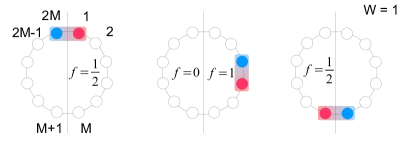
Figure 5: (Color online) Schematics of localization of the two sublattices at the edge crossing point with winding number $w=1$. $N\equiv 2M$ is the number of unit cells. Each empty dot represents a unit cell. Red and blue dots represent the $A$ and $B$ sublattice wavefunctions of a Wannier state, respectively. The $A$ sublattice is $w=1$ unit cell ahead of the $B$ sublattice. The Wannier state itself is represented as the box around the colored dots. The complete set of Wannier states is generated by shifting a given Wannier state by integer number of unit cells. Since the two sublattices are localized on neighboring unit cells, the Wannier center, which is their average spatial location, is a half odd-integer. The entanglement eigenstates are qualitatively the same as the Wannier states in terms of sublattice localization, although quantitatively the wavefunctions do have projections onto neighboring Wannier states. If the bipartition cut passes through the box (representing the dominant Wannier state projection of the entanglement eigenstate), then each half has only one sublattice manifesting as a $f={\textstyle{1\over 2}}$ occupancy mode. For periodic systems, there are two such modes, illustrated in the left and right panels. Clearly, only the right panel survives as entanglement $f={\textstyle{1\over 2}}$ mode for open boundary systems. The middle panel is a Wannier state whose localization does not cross the bipartition cut. Qualitatively, it represents an entanglement state close to $f=0$ for the left half system and $f=1$ for the right half system, cf. the light blue line in Fig. 4.

There is an interesting consequence in entanglement spectrum due to the $w$-separation between the sublattices. For a general $|w|\neq 1$, it is obvious from Fig. 5 that for each Wannier state, there are $w$ ways to place an entanglement cut that will assign the two sublattice wave packets into different halves, generating a half occupancy mode. Thus in the thermodynamic limit, there are $2w$ modes of $f={\textstyle{1\over 2}}$ with a periodic-boundary system, and $w$ such modes with an open-boundary system. We have confirmed this with hand-crafted $\varphi(k_{2})$ relations, e.g., $\varphi(k_{2})=w\sqrt{2\pi k_{2}}$. This agrees with the general observation that the number of entanglement spectral flows is given by the Chern index.

II.3 Armchair Edge

The armchair edge is more conveniently described by a new set of primitive vectors $\vec{a}_{i}^{\,\prime}$:

$$\vec{a}_{1}^{\,\prime}=\vec{a}_{1}+\vec{a}_{2}\quad,\quad\vec{a}_{2}^{\,\prime}=\vec{a}_{2}\ ,$$ (60)

and the associated Bloch phases $k_{i}^{\prime}=\vec{k}\cdot\vec{a}_{i}^{\,\prime}$ are

$$k_{1}^{\prime}=k_{1}+k_{2}\quad,\quad k_{2}^{\prime}=k_{2}\ .$$ (61)

The armchair edge is parallel to $\vec{a}_{1}^{\,\prime}$ and the corresponding open boundary Hamiltonian can be parameterized by $k_{1}^{\prime}$. The bulk Hamiltonian is still eqn. 3. When $k_{1}^{\prime}=0$, then $B_{y}=0$ and the path of $\vec{B}$ upon varying $k_{2}^{\prime}$ is on the $zx$ plane. Thus in the topological phase (origin inside the path), one can repeat the same analysis as done for the zigzag edge and conclude that at $k_{1}^{\prime}=0$, the Berry phase is $\pi$, and the entanglement occupancy is ${\textstyle{1\over 2}}$. We have confirmed these numerically. As for the energy edge modes, while there appear to be no explicit solution, we have confirmed numerically that they still cross at this coplanar point.

From eqn. 3, $B_{y}/(1+B_{x})=\tan(k_{1}^{\prime}/2)$, i.e., the projection of $\vec{B}$ onto the $xy$ plane is a line passing through the point $(B_{x},B_{y})=(-1,0)$, so the path of $\vec{B}$ is always coplanar for any fixed $k_{1}^{\prime}$, but only the one with $k_{1}^{\prime}=0$ has the origin on the same plane. Thus unlike the zigzag edge case, there exists no other $k_{1}^{\prime}$ points whose Berry phase can be related solely to the winding of a planar $\vec{B}$ path.

III Bilayer Haldane Model

A bilayer extension can be constructed by Bernal stacking two monolayers with a vertical interlayer hopping $t_{\perp}$, as shown in Fig. 6. $t_{\perp}$ couples any $A$ site with the $D$ site above it. The Haldane phases of the two layers, $\phi$ for $AB$ and $\chi$ for $CD$, are taken to be independent. Semenoff masses for the four sites are $m_{A}=-m_{B}=-m_{C}=m_{D}=m$. Both layers have the same second neighbor hoppings $t_{i},i=1,2,3$. The bulk Hamiltonian is thus

$$H(\vec{k})=\begin{pmatrix}H_{AB}(\vec{k})&\tilde{T}\\ \tilde{T}^{\rm T}&H_{CD}(\vec{k})\end{pmatrix}\quad,\quad\tilde{T}=\begin{pmatrix}0&t_{\perp}\\ 0&0\end{pmatrix}$$ (62)

where $H_{AB}$ and $H_{CD}$ are given by eqns. 2 and 3 with different parameters $H_{AB}=H(\phi,m)$ and $H_{CD}=H(\chi,-m)$. Superscript $t$ denotes matrix transposition. The two layers individually can have different Chern indices. Thus as long as the central gap does not close when $t_{\perp}$ is turned on, the total Chern number should be given by the sum of those of the individual layers. This is numerically verified, see Fig. 7, where we plot open boundary energy spectrum and entanglement occupancy spectrum.

An interesting case is when $\phi=-\chi$ (Fig. 7(d)). The bulk Hamiltonian is mapped to its complex conjugate under inversion,

$$\mathcal{I}\,H(\vec{k})\>\mathcal{I}=H^{*}(\vec{k})\quad,\quad\mathcal{I}\equiv\begin{pmatrix}&&&1\\ &&1\\ &1\\ 1\end{pmatrix}\ .$$ (63)

We shall refer to this as the $\mathcal{I^{*}}$ symmetry. If both layers are individually topological, their Chern numbers are opposite and there is no gapless edge mode. The entanglement occupancy spectrum also exhibits no spectral flow, but unlike the generic $\phi\neq-\chi$ case, there are protected half occupancy modes occuring at the $k_{1}$ very close to the edge crossing $k_{\rm c}$ point of the corresponding monolayer (clearly, they must be identical when $t_{\perp}=0$). This is reminiscent of the $\mathbb{Z}_{2}$ inversion-symmetric topological insulatorsHughes et al. (2011), which also shows protected $f={\textstyle{1\over 2}}$ entanglement modes without gapless edge modes in the energy spectrum. An essential difference is that there, they only occur at inversion-symmetric $k_{1}=0$ or $\pi$ points because inversion relates $H(\vec{k})$ to $H(-\vec{k})$.

Given the connection between entanglement spectrum and Wannier centers, the question naturally arises as to how the latter would behave in the presence of $\mathcal{I^{*}}$ symmetry. We shall address this question in this section.

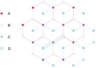
Figure 6: (Color online) Bilayer model. $A$,$B$, $C$ and $D$ label sublattice sites, where $A$ and $B$ are on the first layer (solid line lattice) and $C$ and $D$ on the second (dashed line lattice). Box represents a unit cell. Interlayer hopping is between $A$ and the $D$ on top of it.

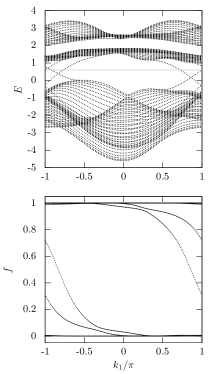
(a)  $\phi=0.3\pi$, $\chi=0.4\pi$

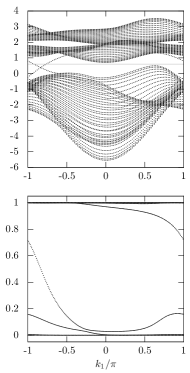
(b)  $\phi=0.3\pi$, $\chi=0.05\pi$

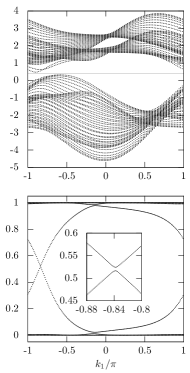
(c)  $\phi=0.3\pi$, $\chi=-0.4\pi$

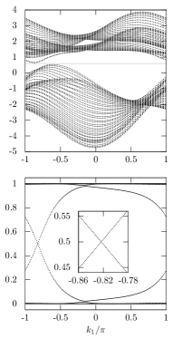
(d)  $\phi=0.3\pi$, $\chi=-0.3\pi$

Figure 7: Open boundary energy spectrum (upper panel) vs. entanglement occupancy spectrum (lower panel) of the bilayer model. Gray line indicates Fermi level. Parameters used are $[t_{1},t_{2},t_{3}]=[0.3,0.4,0.5]$, $m=1$, and $t_{\perp}=0.5$. The Haldane phases $\phi$ and $\chi$ for each case are given in the subfigure title. (a) Both layers have Chern number $C=1$, giving a total $\sum C=2$. The entanglement occupancy spectrum has two flowing branches, each taking about one $k_{1}$ cycle ($k_{1}\rightarrow k_{1}+2\pi$) to flow from $f\simeq 1$ to $f\simeq 0$. (b) $AB$ layer has $C=1$ and $CD$ layer has $C=0$, hense $\sum C=1$. Note the avoided crossing near $f\simeq 0.1$: If the two Haldane layers are not coupled, the crossing will not be avoided and one ends up having one flowing branch (which takes one $k_{1}$ cycle to flow from $f\simeq 1$ to $f\simeq 0$, see (a)) and another trivial branch. The avoided crossing effectively merges the two branches into a single branch which now takes about two $k_{1}$ cycles to flow from $f\simeq 1$ to $f\simeq 0$. (c) and (d): $AB$ and $CD$ individually have opposite Chern indices. (c) Generic case where $\phi$ and $\chi$ are not related. (d) $\mathcal{I^{*}}$-symmetric case with $\phi=-\chi$. Insets: details around half occupancy $f={\textstyle{1\over 2}}$. In (d), the crossing at $f={\textstyle{1\over 2}}$ is not lifted by the $t_{\perp}$ hopping. Crossings near $f=1$ and $0$ are avoided in both (c) and (d). Note that in all cases the number of gapless edge modes at a given boundary is given by $\sum C$, so is the number of entanglement spectral flows. (d) has no flow due to avoided crossing near $f=0$ and $1$.

III.1 Non-Abelian Wannier centers and Wilson loop phases

The Haldane bilayer has $\nu=2$ bands filled at half filling. For adiabatic evolution of $\nu$ bands, the concept of Berry connection (“geometrical vector potential”) generalizes to a $\nu\times\nu$ Berry connection matrix (“non-Abelian gauge field”)Wilczek and Zee (1984),

$$\hat{A}_{ab}=\langle\psi_{k}^{a}|\,i\,\partial_{k}\,|\psi_{k}^{b}\rangle$$ (64)

where $|\psi_{k}^{a}\rangle$ is the internal-space eigenstate at $k$ of the $a^{\rm th}$ band, etc. The Wilson loop, also a $\nu\times\nu$ matrix, is defined as

$$\hat{\mathcal{W}}={\raise 2.5pt\hbox{$\wp$}}\exp\left\{i\!\int\limits_{0}^{2\pi}\!\!dk\,\hat{A}(k)\right\}$$ (65)

where $\wp$ denotes path ordering. The phases of its eigenvalues play the role of Berry phase.

The Wannier states and Wannier centers can still be defined as the eigenstates and eigenvalues of the band-projected position operator eqn. 38, where $\mathcal{G}$ now consists of $\nu$ bands, $\mathcal{G}=\sum_{a=1}^{\nu}\sum_{k}|\Psi_{k}^{a}\rangle\langle\Psi_{k}^{a}|$, and $|\Psi_{k}^{a}\rangle~{}=~{}|k\rangle~{}\otimes~{}|\psi_{k}^{a}\rangle$ is eigenstate of the $a^{\rm th}$ band below Fermi level. One then finds that as the number of lattice sites $N\rightarrow\infty$, the Wannier centers are given by Qi (2011)

$$x_{w,I}={\gamma_{w}\over 2\pi}+I$$ (66)

where $I$ is an integer labeling the corresponding unit cell, and $\gamma_{w}$ is given by the phase of the $w^{\rm th}$ eigenvalue of $\hat{\mathcal{W}}$,

$$\hat{\mathcal{W}}\,\mathbf{g}_{w}=e^{i\gamma_{w}}\,\mathbf{g}_{w}\quad,\quad w=1,2,\ldots,\nu\ .$$ (67)

The $\nu$ bands recombine to yield $\nu$ Wannier functions associated with each unit cell. When $\nu=1$, this reduces to eqn. 39.

In the finite $N$ case, it is more convenient to replace the position operator $R=\hat{Y}\otimes\mathbb{I}$ with the $k$-space translation operator $\exp(i\hat{Y}\delta k)\otimes\mathbb{I}$ where $\delta k=2\pi/N$ is the $k$-space step Yu et al. (2011). The object of concern is instead (cf. derivation of eqn. 202)

$$\hat{\mathbb{W}}=P_{k^{\vphantom{\dagger}}_{N}}P_{k^{\vphantom{\dagger}}_{N-1}}P_{k^{\vphantom{\dagger}}_{N-2}}\cdots P_{k^{\vphantom{\dagger}}_{2}}P_{k^{\vphantom{\dagger}}_{1}}P_{k^{\vphantom{\dagger}}_{N}}\,.$$ (68)

where $k_{n}=n\,\delta k$ with $n=1,2,\ldots,N$, and $P_{k_{n}}=\sum_{a=1}^{\nu}|\psi_{k_{n}}^{a}\rangle\langle\psi_{k_{n}}^{a}|$ is the internal-space projector onto the occupied bands at $k$. Note that this object is basis-independent—in particular, it is oblivious to the phase choice of the $|\psi_{k}^{a}\rangle$ states, which is advantageous for numerics. Note also that the dimension of $P_{k}$ and hence of $\hat{\mathbb{W}}$ is the number of total bands $q$ whereas that of $\hat{\mathcal{W}}$ is $\nu$, the number of occupied bands. However, $\hat{\mathcal{W}}$ is essentially the nonzero block of $\hat{\mathbb{W}}$ (cf. eqn. 203), hence they have the same (complex) nonzero eigenvalues $\{\rho_{w}\,e^{i\gamma_{w}}\}$ where $w=1,2,\ldots,\nu$. The amplitudes $\rho_{w}$ will deviate from unity due to discretization. The phases $\gamma_{w}$ will be interpreted as the Wannier center offsets as in eqn. 66. See Appendix C for details.

$\hat{\mathbb{W}}$ in the form of eqn. 68 – as a product of occupied band projectors over the period of $k$ – is also known as a monodromy and has been used in analyzing e.g. inversion-symmetric $\mathbb{Z}_{2}$ topological insulators Hughes et al. (2011). One question is whether or not it matters to break up the Wilson loop at some $k$ point other than $k=0$. The answer is no. This is because the eigenvalues of a product of (possibly non-commuting) projectors are invariant under cyclic permution of these projectors. We prove it in Appendix D.

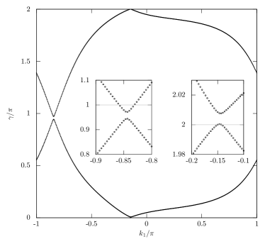
(a)  $\phi=0.3\pi$, $\chi=-0.4\pi$

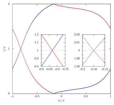
(b)  $\phi=0.3\pi$, $\chi=-0.3\pi$

Figure 8: (Color online) Non-abelian Wilson loop phases. Haldane phases are given in subfigure titles. Other parameters used are the same as in Fig. 7. Insets: details around $\gamma=\pi$ and $2\pi$. (a) has avoided crossings near both $\gamma=\pi$ and $2\pi$, but (b) has no avoided crossings. The red dots in (b) can be computed by eqn. 80. The blue dots are given by their negatives (shifted by $2\pi$).

III.2 Wilson loop phase of the $\mathcal{I^{*}}$-symmetric bilayer Haldane model

III.2.1 $\mathcal{I^{*}}$-symmetric bilayer eigenstates

Upon swapping the $C$ and $D$ rows and columns, the Hamiltonian eqn. 62 becomes (suppressing $k_{1}$ dependence)

$$H=\omega\,\mathbb{I}+\begin{pmatrix}M&T\\ T^{*}&M^{*}\end{pmatrix}$$ (69)

$$M=\vec{B}\cdot\vec{\sigma}\quad,\quad T=T^{*}=\begin{pmatrix}t_{\perp}&0\\ 0&0\end{pmatrix}\ ,$$ (70)

where $\omega$ and $\vec{B}$ are given by eqn. 3. The form of eqn. 69 means its eigenstates are of the form

$$|\psi\rangle=\begin{pmatrix}|u\rangle\\ |u^{*}\rangle\end{pmatrix}$$ (71)

where $|u\rangle=\bigl{(}\begin{smallmatrix}u_{1}\\ u_{2}\end{smallmatrix}\bigr{)}$ is a two-component column vector. The eigenvalue equation is thus

$$M|u\rangle+T|u^{*}\rangle=\varepsilon|u\rangle\ .$$ (72)

Since interlayer hopping is restricted to $A$ and $D$ sites, $T|u^{*}\rangle$ only depend on $u_{1}$, thus one may always adopt a phase choice of $|u\rangle$ such that $u_{1}$ is either real, in which case $T|u^{*}\rangle=T|u\rangle$, or imaginary, in which case $T|u^{*}\rangle=-T|u\rangle$. The eigenvalues of $H$ consequently comprise those of $2\times 2$ $H^{\pm}$ defined as

$$H^{\pm}\equiv\omega\,\mathbb{I}+M\pm T=\omega_{\pm}\,\mathbb{I}+\vec{B}_{\pm}\cdot\vec{\sigma}\ ,$$ (73)

$$\omega_{\pm}=\omega\pm{\textstyle{1\over 2}}t_{\perp}\ ,$$ (74)

$$\vec{B}_{\pm}=\bigl{(}B_{x},B_{y},B_{z}\pm{\textstyle{1\over 2}}t_{\perp}\bigr{)}=\big{(}|B_{\pm}|,\vartheta^{\pm},\varphi\big{)}$$ (75)

where $\big{(}|B_{\pm}|,\vartheta^{\pm},\varphi\big{)}$ are the spherical polar coordinates of $\vec{B}_{\pm}$. The role of $t_{\perp}$ is two-fold: by modifying $\omega$, it splits the two monolayer copies; by modifying $B_{z}$, it also changes the level splitting of each monolayer. Thus as $t_{\perp}$ is increased from $0$ adiabatically, it is possible to rearrange the order of the monolayer bands. Here we shall focus on the case where the central gap is never closed during $0\rightarrow t_{\perp}$, so that the occupied bands $|\psi^{\pm}(\vec{k})\rangle$ at half filling are generated by the isospin-down states of $H^{\pm}$, viz.,

$$|\psi^{+}\rangle={\textstyle{i\over\sqrt{2}}}D_{z}(\varphi)\begin{pmatrix}\phantom{+}|\vartheta^{+}\rangle\\ -|\vartheta^{+}\rangle\end{pmatrix}\ ,$$

$$|\psi^{-}\rangle={\textstyle{1\over\sqrt{2}}}D_{z}(\varphi)\begin{pmatrix}|\vartheta^{-}\rangle\\ |\vartheta^{-}\rangle\end{pmatrix}\ ,$$ (76)

where $D_{z}(\varphi)=\textsf{diag}(1,e^{i\varphi},1,e^{-i\varphi})$ and $|\vartheta^{\pm}\rangle=\begin{pmatrix}-\sin{\textstyle{\vartheta^{\pm}\over 2}}\\ \cos{\textstyle{\vartheta^{\pm}\over 2}}\end{pmatrix}$ are purely real. Note that $|\psi^{\pm}\rangle$ have the prescribed form $\begin{pmatrix}|u\rangle^{\phantom{*}}\\ |u^{*}\rangle\end{pmatrix}$ with $u_{1}$ imaginary for $|\psi^{+}\rangle$ and real for $|\psi^{-}\rangle$.

III.2.2 Wilson loop phases

Fig. 8 plots the Wilson loop phases of the Haldane bilayer where the two layers have opposite Chern indices. In the generic $\phi\neq-\chi$ case (Fig. 8(a)), both $\gamma_{w}$ levels exhibit no flow over the period of $k_{1}$ due to avoided crossings, which is similar to the corresponding entanglement spectrum (Fig. 7(c)). In the $\mathcal{I^{*}}$-symmetric case where $\phi=-\chi$, none of the crossings at $\gamma=0$ and $\pi$ are avoided, thus both $\gamma_{w}$ levels flow in opposite directions. This is different from the entanglement spectrum (Fig. 7(d)) where the crossing at $f={\textstyle{1\over 2}}$ is preserved, but the crossings near $f=1$ and $0$ are avoided. Unlike the monolayer case, the $f={\textstyle{1\over 2}}$ crossing does not coincide in $k_{1}$ with the $\gamma=\pi$ crossing, although they are very close. This is because one no longer has the analog of a coplanar $k_{1}$ point. We will come back to this point later.

Since the set $\{\gamma_{w}\}$ is periodic as $k_{1}\rightarrow k_{1}+2\pi$, their winding numbers $\bigl{[}\gamma_{w}(2\pi)-\gamma_{w}(0)\bigr{]}/(2\pi)$ must be integers. The question is how to extract them. From eqn. 76, one finds that the Berry connection matrix is purely off-diagonal,

$$\langle\psi^{+}|\partial_{k^{\vphantom{\dagger}}_{2}}|\psi^{+}\rangle =\langle\psi^{-}|\partial_{k^{\vphantom{\dagger}}_{2}}|\psi^{-}\rangle=0\,,$$ (77)

$$\langle\psi^{-}|\partial_{k^{\vphantom{\dagger}}_{2}}|\psi^{+}\rangle =-{\partial\varphi\over\partial k_{2}}\,\cos({\textstyle{1\over 2}}\vartheta^{+})\cos({\textstyle{1\over 2}}\vartheta^{-})\,,$$ (78)

hence

$$\hat{\mathcal{W}}(k_{1})=e^{i\tilde{\gamma}(k_{1})\,\sigma_{y}}\,$$ (79)

$$\tilde{\gamma}(k_{1})=-\!\!\!\int\limits_{\varphi(0)}^{\varphi(2\pi)}\!\!\!d\varphi\,\cos{\textstyle{\vartheta^{+}\over 2}}\cos{\textstyle{\vartheta^{-}\over 2}}\ .$$ (80)

Note that when $t_{\perp}=0$, $\vartheta^{+}=\vartheta^{-}$ and eqn. 80 reduces to eqn. 45. The Wilson loop phases are simply $\pm\tilde{\gamma}$. In Fig. 8(b), red curve corresponds to $+\tilde{\gamma}$ and blue to $-\tilde{\gamma}$.

While there are no inversion or time-reversal symmetries protecting the winding of this off-diagonal $\tilde{\gamma}$ (by fixing $\tilde{\gamma}=0$ and $\pi$ at $\mathcal{T}$ or $\mathcal{I}$ symmetric $k_{1}$ points), it is nontheless robust with respect to $t_{\perp}$ as long as the central gap remains open, and is thus given by the corresponding monolayer Chern number ($t_{\perp}=0$ case). To see this, we use the eigenstates of $\hat{\mathcal{W}}$ (cf. eqns. 193 and 194) to construct a set of states,

$$|\eta_{\pm}\rangle =g_{\pm}^{+}\,|\psi^{+}\rangle+g_{\pm}^{-}\,|\psi^{-}\rangle={\textstyle{1\over\sqrt{2}}}\big{\{}|\psi^{+}\rangle\pm i|\psi^{-}\rangle\big{\}}$$ (81)

$$={\textstyle{i\over 2}}D_{z}(\varphi)\begin{pmatrix}|\vartheta^{+}\rangle+|\vartheta^{-}\rangle\\ |\vartheta^{-}\rangle-|\vartheta^{+}\rangle\end{pmatrix}$$ (82)

where $\mathbf{g}_{\pm}=(g_{\pm}^{+},g_{\pm}^{-})^{\rm T}$ are the eigenstates of $\hat{\mathcal{W}}$, in this case, the eigenstates of $\sigma_{y}$. The Berry connection matrix $\hat{A}$ is diagonal in the $|\eta_{\pm}\rangle$ basis, i.e., $\tilde{\gamma}$ is the Berry phase (over $k_{2}$) of the $|\eta_{+}\rangle$ “band”. It is easy to verify that the two layers, $AB$ and $CD$, each contributes exactly one half to $\tilde{\gamma}$. One may thus construct a ficticious two-band model whose occupied band is given by the projection of say $|\eta_{+}\rangle$ onto the $AB$ layer,

$$|-\rangle={\textstyle{1\over\sqrt{2}}}\begin{pmatrix}1\\ &e^{i\varphi}\end{pmatrix}\bigl{(}|\vartheta^{+}\rangle+|\vartheta^{-}\rangle\bigr{)}\ ,$$ (83)

and the unoccupied band as

$$|+\rangle={\textstyle{1\over\sqrt{2}}}\begin{pmatrix}1\\ &e^{i\varphi}\end{pmatrix}\bigl{(}|\bar{\vartheta}^{+}\rangle-|\bar{\vartheta}^{-}\rangle\bigr{)}\ .$$ (84)

Here, $|\bar{\vartheta}\rangle=\begin{pmatrix}\cos(\vartheta/2)\\ \sin(\vartheta/2)\end{pmatrix}$ are the iso-spin up counterpart of $|\vartheta\rangle$. By construction, $\langle+|-\rangle=0$. The ficticious Hamiltonian is

$$\tilde{H}=\sum_{\vec{k},s=\pm}\varepsilon_{s}(\vec{k})\,|\vec{k}\rangle\langle\vec{k}|\otimes|s(\vec{k})\rangle\langle s(\vec{k})|$$ (85)

where $\varepsilon_{+}$ can be chosen as (say) the lower energy of the two unoccupied bilayer bands, and $\varepsilon_{-}$ as the higher energy of the two occupied bilayer bands. Then $\tilde{\gamma}(k_{1})$ is the Berry phase of $\tilde{H}$, and its winding number is the same as the monolayer Haldane model as long as $t_{\perp}$ does not collapse the bilayer central gap. The reason why the point of $\tilde{\gamma}=\pi$ is very close to but no longer coincide with where the $f={\textstyle{1\over 2}}$ entanglement mode occurs, which was the case for monolayers, is that if one maps the state of eqn. 83 back to a vector $\vec{B}$, with its azimuth as $\varphi$ and its polar angle being some sort of average of $\vartheta^{+}$ and $\vartheta^{-}$, then around the monolayer $k_{\rm c}$, the path of $\vec{B}$ comes close to coplanarity (yet never exactly so). Since the “temperature” $\beta$ is different for the entanglement and Wannier spectra (cf. eqn. 51), they need different distortions in the $\vec{B}$ path to balance $\beta$ in order to reach their special values.

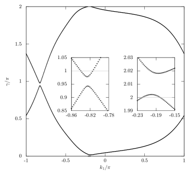
(a)  $\phi=0.3\pi,\chi=-0.4\pi,N_{2}=500$

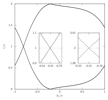
(b)  $\phi=0.3\pi,\chi=-0.3\pi,N_{2}=500$

(c)  $\phi=0.3\pi,\chi=-0.4\pi,N_{2}=10$

(d)  $\phi=0.3\pi,\chi=-0.3\pi,N_{2}=10$

Figure 9: Wilson loop phases of bilayer Haldane model with generic $\mathcal{I^{*}}$-preserving interlayer hopping, and the effect of $k_{2}$ undersampling. Parameters used are $t_{\perp}=0.5$, $\lambda=0.4$, other parameters are the same as in Fig. 7. Insets: details around $\gamma=\pi$ and $2\pi$. (a): $\phi\neq-\chi$, i.e., $\mathcal{I^{*}}$-non-symmetric. (b): $\phi=-\chi$, i.e., $\mathcal{I^{*}}$-symmetric. (c): same as (a) but only use $N_{2}=10$ projectors in eqn. 68. (d): same as (b) but with $N_{2}=10$. Notice that qualitative features do not depend on the number of $k_{2}$ discretization. In particular, $k_{2}$ undersampling does not lift the crossing in the $\mathcal{I^{*}}$-symmetric case.

III.3 Generic $\mathcal{I^{*}}$-preserving interlayer hopping

The reason why $\tilde{\gamma}$ can be extracted from the bilayer Haldane model is because the Berry connections $\hat{A}(\vec{k})$ are proportional to $\sigma_{y}$, and hence are mutually commuting at different $\vec{k}$. This in turn is because the interlayer hopping is only between $A$ and $D$ sites, so that $H$ decomposes into $H^{\pm}$ sectors. Thus while there is a matrix structure, the situation is nontheless Abelian. Still, the $\mathcal{I^{*}}$-symmetric bilayer provides an interesting example where the topological information is not obvious from the open-boundary energy spectrum. The role of the $\mathcal{I^{*}}$ symmetry is in prescribing the eigenstates to a particular form $\bigl{(}\begin{smallmatrix}|u\rangle^{\phantom{*}}\\ |u^{*}\rangle\end{smallmatrix}\bigr{)}$ (after swapping $C$ and $D$ labeling). One question to ask is if the crossings as seen in the Wilson loop phases of the $\mathcal{I^{*}}$-symmetric bilayer is a consequence solely of the $\mathcal{I^{*}}$ symmetry, or if it also depends on the interlayer hopping being restricted to $t_{\perp}$ only. The most general interlayer hopping that preserves $\mathcal{I^{*}}$ is

$$T=\begin{pmatrix}\lambda_{1}&\lambda_{2}\\ \lambda_{2}&\lambda_{3}\end{pmatrix}\quad,\quad\lambda_{i}\in\mathbb{C}\ .$$ (86)

instead of the one used in eqn. 70. In the bilayer stacking, the $B$ sites are surrounded by three “nearest-neighbor” $C$ sites on the other layer, $C$ by $A$, and $D$ by $B$, thus one example of such $T$ matrix is by treating the strength of all these interlayer hoppings as $\lambda$ in addition to the vertical $t_{\perp}$ between $A$ and $D$,

$$\lambda_{1}=t_{\perp}\ ,$$

$$\lambda_{2}=\lambda(1+e^{ik_{1}}+e^{ik_{2}})\ ,$$

$$\lambda_{3}=\lambda(e^{ik_{1}}+e^{ik_{2}}+e^{i(k_{1}+k_{2})})\ .$$ (87)

Although not important for our purpose here, these parameters can be connected to the SWMC model of grapheneNilsson et al. (2008).

$\mathcal{I^{*}}$ symmetry of the Hamiltonian is inherited by the internal-space projector of occupied bands, and hence their product $\hat{\mathbb{W}}$,

$$\mathcal{I}P(\vec{k})\,\mathcal{I}=P^{*}(\vec{k})\quad,\quad\mathcal{I}\,\hat{\mathbb{W}}(k_{1})\,\mathcal{I}=\hat{\mathbb{W}}^{*}(k_{1})\ .$$ (88)

So if $|g_{w}\rangle$ is an eigenstate of $\hat{\mathbb{W}}$ with eigenvalue $\rho_{w}\,e^{i\gamma_{w}}$, then $\mathcal{I}\,|g_{w}\rangle^{*}$ is also an eigenstate with eigenvalue $\rho_{w}\,e^{-i\gamma_{w}}$. Thus the eigenvalues of $\hat{\mathbb{W}}$ come in complex-conjugate pairs. For the bilayer with a general interlayer hopping eqn. 86, while there does not seem to be a way of tracking one of the two $\hat{\mathbb{W}}$ eigenstates (with nonzero $\rho_{w}$) analytically, we do find numerically that the $\{\gamma_{w}\}$ pair flow in opposite directions and cross at $\gamma=0$ and $\pi$ just like the case with $t_{\perp}$-only interlayer hopping, and that their winding numbers are given by the underlying monolayer as long as the bilayer central gap does not collapse when turning on $t_{\perp}$ and $\lambda$. Fig. 9(b) plots a $\mathcal{I^{*}}$-symmetric case with $T$ given by $t_{\perp}=0.5$ and $\lambda=0.4$. Compare with Fig. 9(a) where $\phi\neq-\chi$ and the flows are broken near $\gamma=\pi$ and $2\pi$.

An interesting observation made possible by expressing the Wilson loop as a product of projectors is how the topological and non-topological cases behave with an undersampling of $k^{\vphantom{\dagger}}_{\parallel}$, that is, when the number of projectors used in eqn. 68 is reduced. For example, if one were to reduce $N$ projectors to say $N/3$, it is equivalent to replacing every two out of three projectors in the monodromy by a unity operator, thereby allowing wavefunctions to leak into unoccupied states when “propagating” from $k_{i}$ to $k_{i-3}$. Of course $\hat{\mathcal{W}}$ ceases to be unitary due to the leakage, which is just the reason why $\rho_{w}<1$ in the finite $N$ case. A somewhat unexpected behavior is that the Wilson loop phases in the $\mathcal{I^{*}}$-symmetric case now become degenerate for an extended region of $k_{1}$ values at $\gamma=\pi$ and $0$, as opposed to crossing at discrete points in the $N\rightarrow\infty$ limit. The eigenvalues there are simply real numbers, which are their own conjugates and thus not ruled out by the $\mathcal{I^{*}}$ symmetry. Note however that the two real solutions are not required to be the same—indeed they are different for finite $N$ and only approaches $\pm 1$ as $N\rightarrow\infty$ per unitarity of $\hat{\mathcal{W}}$. No such phase degeneracy is observed for the generic $\mathcal{I^{*}}$-asymmetric cases, where the phase flows still exhibit avoided crossing. The topological signature is in this sense more prominent away from the thermodynamic limit, unlike e.g. the crossing of the monolayer energy edge states which in general is a thermodynamic limit result.

III.4 Relation with a $\mathbb{Z}_{2}$ inversion-symmetric TI

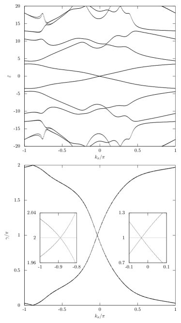
Figure 10: $\mathcal{I^{*}}$-symmetric HPB model with broken inversion. Top panel: periodic boundary entanglement quasi-energy. Bottom panel: Wilson loop phases. Parameters: $m=1.1$, $(\lambda_{1},\lambda_{2},\lambda_{3})=(0.7,0.5,0)$. Since the $\mathcal{I^{*}}$ symmetry is preserved, the model still retains its nontrivial topology: in the entanglement spectrum, although there is no spectral flow, the $\tilde{\varepsilon}=0$ mode, which now is slightly shifted away from $k_{x}=0$, is still robust with no avoided crossing; for the Wilson loop phases, the two branches still wind in opposite directions and intersect at $\gamma=0$ and $\pi$, but the crossings are no longer pinned at $k_{x}=0$ or $\pi$. Insets: details near $\gamma=\pi$ and $2\pi$.

Hughes et. al. studied a $\mathbb{Z}_{2}$ inversion-symmetric TI model (HPB model) Hughes et al. (2011),

$$H(\vec{k})=\sin k_{x}\Gamma_{1}+\sin k_{y}\Gamma_{2}+M(\vec{k})\Gamma_{0}+B_{x}\Gamma_{B}\ ,$$ (89)

$$M(k)\equiv 2-m-\cos k_{x}-\cos k_{y}\ ,$$ (90)

$$\Gamma_{1}=\sigma_{z}\otimes\tau_{x}\quad,\quad\Gamma_{2}=\mathbb{I}\otimes\tau_{y}\ ,$$ (91)

$$\Gamma_{0}=\mathbb{I}\otimes\tau_{z}\quad,\quad\Gamma_{B}=\sigma_{x}\otimes\left(\begin{smallmatrix}1\\ &0\end{smallmatrix}\right)\ .$$ (92)

Here, both $\sigma_{i}$ and $\tau_{i}$ are the Pauli matrices, $\sigma_{i}$ act on the spin indices and $\tau_{i}$ on the orbital indices. The HPB model is built from the BHZ quantum spin Hall model Bernevig et al. (2006) by adding the $\Gamma_{B}$ term which breaks time-reversal but preserves inversion: the inversion operation is defined as $\mathcal{P}\equiv\Gamma_{0}$ such that $\mathcal{P}H(\vec{k})\,\mathcal{P}=H(-\vec{k})$. The authors showed that it has a $\mathbb{Z}_{2}$ topological index protected by the $\mathcal{P}$-symmetry.

The HPB model is also $\mathcal{I^{*}}$-symmetric: $\mathcal{I}=\sigma_{x}\otimes\tau_{z}$ such that $\mathcal{I}H(\vec{k})\,\mathcal{I}=H^{*}(\vec{k})$. In fact this is the mirror symmetry as noted by the same authors in Ref. Hughes et al., 2011. The $\mathcal{T}$-breaking term $B_{x}$ plays the role of $t_{\perp}$ of the bilayer model, therefore the model can be cast into the form of eqn. 69 by rotating $(\tau_{x},\tau_{y})$ to $(\tau_{y},-\tau_{x})$. One can then solve it analytically and analyze its Wannier centers in the same way as the bilayer model. Its $\mathbb{Z}_{2}$ index is equivalent to the winding number of $\tilde{\gamma}$, and is inherited from the “monolayer” (individual spin species) as long as the central gap does not collapse.

It turns out for this particular model, one can choose to break either $\mathcal{P}$ or $\mathcal{I^{*}}$ (but not both) and still retain the nontrivial topology. Here we only consider breaking the $\mathcal{P}$, for as long as it is preserved, the proof of Ref. Hughes et al., 2011 applies. To break $\mathcal{P}$, we add in an $\mathcal{I^{*}}$-symmetric “spin-flipping” hopping. The most general form is to replace the $B_{x}\,\Gamma_{B}$ term in eqn. 89 by

$$\begin{pmatrix}\mathbf{0}&T\\ T^{\dagger}&\mathbf{0}\end{pmatrix}\quad,\quad T=\begin{pmatrix}\lambda_{1}&\lambda_{2}\\ -\lambda_{2}&\lambda_{3}\end{pmatrix}$$ (93)

where again $\lambda_{i}$ are complex numbers which could have $\vec{k}$ dependence. The extra “$-$” sign in $T$ as compared with the bilayer case (eqn. 86) will drop after the aformentioned $(\tau_{x},\tau_{y})\rightarrow(\tau_{y},-\tau_{x})$ rotation. One can easily verify that the condition for inversion symmetry to also hold is $(\lambda_{1},\lambda_{2},\lambda_{3})_{-\vec{k}}=(\lambda_{1},-\lambda_{2},\lambda_{3})_{\vec{k}}$.

Fig. 10 plots the entanglement spectrum and Wilson loop phases of an $\mathcal{I^{*}}$-symmetric HPB model with broken inversion symmetry, $m=1.1$, $(\lambda_{1},\lambda_{2},\lambda_{3})=(0.7,0.5,0)$. The topological signatures still persist: the entanglement quasi-energy spectrum exhibit robust zero modes, and the Wilson loop phases flow in opposite directions and cross at $\gamma=0$ and $\pi$. Since the $\lambda_{2}$ term explicitly breaks $\mathcal{P}$, the $k_{x}$ points where they occur are no longer pinned at symmetry-invariant points.

IV Summary

We have studied the monolayer and bilayer Haldane models and identified several topological signatures from the real space perspective. The monolayer zigzag edge modes can be analytically solved using the Ansatz that the wavefunctions of its $A$ and $B$ sublattices are proportional. This particular form poses restrictions on the boundary condition which can no longer be prescribed (as e.g. an open boundary) but must be solved self-consistenly, and the edge state is recognized as an open boundary one when the “tunnelling strength” $\rho$ of the two boundaries approaches zero in the thermodynamic limit. Using the edge solution, the transverse momentum $k_{1}=k_{\rm c}$ at which the two edge modes cross can be identified as the coplanar point of the $\vec{B}$ vector that generates the bulk Hamiltonian $H=\omega+\vec{B}\cdot\vec{\sigma}$—that is, at this point, varying the longitudinal momentum $k_{2}$ from $0$ to $2\pi$ will drive $\vec{B}$ in a closed path on a plane that passes through the origin. The problem of mapping the $2$-D Brillouin zone $(k_{1},k_{2})$ to the sphere $\vec{B}(k_{1},k_{2})$ is thus reduced to a $1$-D mapping from $k_{2}$ to the ring $\vec{B}(k_{\rm c},k_{2})$, and the bulk Chern index reduces to the winding number of the $\vec{B}$ ring around the origin.

Interestingly, at $k_{\rm c}$, both the entanglement spectrum and the Wannier centers exhibit crossings similar to the edge modes. If one treats the entanglement spectrum as the bipartition coarse graining of the Wannier centers, then there is a continuous parameterization $\beta$ such that the eigenvalues $\{r_{a}\}$ of a band-projected real space operator $\mathcal{G}R_{\beta}\,\mathcal{G}$ correspond to the entanglement spectrum at one limit $\beta\rightarrow\infty$, and to the Wannier centers at the other limit $\beta\rightarrow 0$. The crossing at $k_{\rm c}$ is universal in that for arbitrary $\beta$, there always exist $r_{a}$ levels fixed at $r_{a}=(N+1)/2$, where $N$ is the number of unit cells in the longitudinal direction $\vec{a}_{2}$. The special $r_{a}$ value translates to half occupancy $f={\textstyle{1\over 2}}$ in the entanglement case, and to a state localized right in the middle of the $N$-cell chain in the Wannier case. This universal crossing can be traced back to the $\vec{B}$ coplanarity because the two sublattices (after an internal rotation) are localized in different unit cells with the separation given by the winding number $w$ of the $\vec{B}$ ring, thus their average center is a half-odd-integer if $w$ is odd, giving rise to the special Wannier center, and an entanglement cut placed in between them will assign the two sublattices to different halves of the bipartite, yielding an $f={\textstyle{1\over 2}}$ entanglement occupancy in each half.

The Haldane bilayer is constructed by Bernal-stacking two monolayers and allow vertical interlayer hopping $t_{\perp}$. Without exception, the Chern index of bilayer at half filling is the sum of those of the individual monolayers, which also manifests as the number of entanglement spectral flows. A special case is when the two monolayers individually have nonvanishing Chern indices but are opposite to each other: the nontrivial topology survives in a sense if their parameters are exactly opposite such that the bilayer bulk Hamiltonian is mapped to its complex conjugate by inversion, $\mathcal{I}H(\vec{k}\mathcal{)}I=H^{*}(\vec{k})$ ($\mathcal{I^{*}}$ symmetry): while there is no gapless edge modes and no entanglement spectral flow, the entanglement spectrum does exhibit protected $f={\textstyle{1\over 2}}$ modes. It becomes more prominent in the Wannier center (Wilson loop phases) spectrum, where two branches start to flow in opposite directions with the magnitude of their winding number given by the monolayer Chern index. The flow is robust as long as the central gap of the bilayer does not collapse when $t_{\perp}$ is varied. The role of $\mathcal{I^{*}}$ symmetry is further confirmed numerically by adding in $\mathcal{I^{*}}$-preserving generic interlayer hopping. We also found that unlike the monolayer open boundary edge spectrum whose gapless crossing is a thermodynamic limit result, the crossing of the opposing Wilson loop phase flows are more prominent as the number of unit cells $N$ in the $\vec{a}_{2}$ direction is reduced: they are now degenerate for an extended region of $k_{1}$ instead of crossing at discrete points. This does not happen for the topologically trivial case where $\mathcal{I^{*}}$ is broken.

The flow-less entanglement spectrum with protected midgap modes is reminiscent of the $\mathbb{Z}_{2}$ inversion-symmetric topological insulators, with the essential difference that the midgap modes there are pinned at inversion-invariant $k$ points. We looked at one such model studied in Ref. Hughes et al., 2011. This particular model has both inversion ($\mathcal{P}$) and mirror symmetry. The latter coincides mathematically with the $\mathcal{I^{*}}$ symmetry, rendering the model solvable in the same way as the $t_{\perp}$-only bilayer. The nontrivial topology as captured by the $\mathbb{Z}_{2}$ index survives as long as either of $\mathcal{P}$ and $\mathcal{I^{*}}$ is preserved. The former case falls within the analysis of Ref. Hughes et al., 2011. We illustrated the latter by adding in $\mathcal{I^{*}}$-preserving perturbations that break $\mathcal{P}$. Such a perturbations shift the $f={\textstyle{1\over 2}}$ modes and the $\pi$ Wilson loop phases away from the $\mathcal{P}$-invariant $k$ points but does not generate any avoided crossing.

Both the BHZ quantum spin Hall model and the HPB inversion-symmetric TI model inherit their $\mathbb{Z}_{2}$ index from the Chern index of the underlying single spin species, and from the point of view of the Wilson loop phases, are topologically equivalent to the situations where the coupling between the two spin species are turned off, although for the HPB model this qualitatively changes the edge spectrum behavior. Mathematically the question becomes how the interspin coupling (or interlayer coupling in the bilayer case) influences the flow pattern of the Wilson loop phases, and what kind of coupling does not degenerate the pattern to the trivial case (e.g., that of a unity operator). The bilayer Haldane model shows that there are other types of coupling which break both time-reversal and inversion and yet still result in a nontrivial topology.

V Acknowledgments

This work was supported by the NSF through grant DMR-1007028.

Appendix A Details of Monolayer Zigzag Edge States

A.1 Edge solution

From 16, we note that as $k_{1}\rightarrow-k_{1}$,

$$\quad v_{1}(-k_{1})=v_{2}^{*}(k_{1})\quad,\quad p_{1}(-k_{1})=p_{1}(k_{1})$$ (94)

Eqn. 21 gives two equations (the ratio $r$ itself being yet undetermined) with two unknowns, $\lambda$ and $\varepsilon$, for each $k_{1}$ value. The second equality of eqn. 21 does not involve $\varepsilon$, and can be used to solve for $\lambda$,

$$p^{\vphantom{\dagger}}_{2}\,v^{\vphantom{\dagger}}_{2}\lambda^{2}+(v^{\vphantom{\dagger}}_{2}v_{1}^{*}-v^{\vphantom{\dagger}}_{1}v_{2}^{*}+p_{2}^{2})\,\lambda+p^{\vphantom{\dagger}}_{2}\,v_{1}^{*}=0,$$ (95)

This yields eqns. 22 and 23. Note that sending $\lambda\leftrightarrow\lambda^{-1}$ and $v_{1}\leftrightarrow v_{2}^{*}$ keeps eqn. 95 invariant, thus together with eqn. 94, one gets

$$d(k)=d(-k),$$ (96)

$$\lambda_{+}(k)=\lambda_{-}^{-1}(-k),\quad r_{+}(k)=r_{-}^{-1}(-k).$$ (97)

To solve for $\varepsilon$, we use a simple fact about ratios: if $r=x_{1}/y_{1}=x_{2}/y_{2}$, then $r$ is preserved by arbitrary linear combination of numerators and denominators, $r=(ax_{1}+bx_{2})/(ay_{1}+by_{2})$, except the unfortunate choice that makes $ax_{1}+bx_{2}=0$. Applying to eqn. 21, we get

$$r={p_{2}h_{1}-p_{2}\varepsilon-2p_{1}\textsf{Re}\,v_{1}\over p_{2}h_{2}-p_{2}\varepsilon-2p_{1}\textsf{Re}\,v_{2}}$$ (98)

where Re indicates real part. This gives the two solutions of $\varepsilon$, eqn. 24, in terms of $r_{\pm}$ as solved in eqn. 23. Similar to eqn. 96,

$$\varepsilon_{+}(m,k_{1})=\varepsilon_{-}(-m,-k_{1}).$$ (99)

The bulk spectrum has the same inversion property which is easily verified from eqn. 3.

In the text (eqn. 27) we mentioned that $r_{\pm}$ is real if the discriminant $\Delta$ is non-negative. The reality of $r_{\pm}$ (eqn. 27) in turn has the following implication: Using $r=r^{*}$ and eqn. 21,

$$r={v_{1}^{*}+\lambda p_{2}\over v_{2}^{*}}=r^{*}={\lambda^{*}v_{1}^{*}\over\lambda^{*}v_{2}^{*}+p_{2}}\implies r=-|\lambda|^{2},$$ (100)

which can also be checked explicitly using eqn. 23. Notice that this applies to the singular case, eqn. 26, as well.

That we can get eqn. 100 is actually fortunate, for otherwise there will be no twisted boundary consistent with the Ansatz. We will come back to this point later when deriving the eigenstates.

A.2 Edge crossing point

To derive the edge crossing point, we note that according to eqn. 23, the ratio $r$ depends on the branch: in general $r_{+}\neq r_{-}$. But eqn. 98 implies that at the edge crossing point(s), $r_{+}=r_{-}$. It would seem the latter is satisfied only when the discriminant $\Delta=0$, but one can easily verify from Fig. 2 that these do not correspond to the edge crossing points. In fact, there is a range of parameters in the topological phase where $\Delta$ is always positive, e.g., $t_{1}=t_{2}=t_{3}=0.3$, $m=\phi/\pi=0.5$. Recall that in deriving eqn. 98, we used linear combinations of denominators and numerators of the three ratios in eqn. 21, the validity of which requires these combinations to be non-singular (cf. discussion leading to eqn.98). Thus the only way for eqns. 23 and 98 to be consistent—the former implying $r_{+}\neq r_{-}$, the latter implying otherwise—is for the linear combinations of both the denominators and the numerators to be singular, viz.,

$$p_{2}(h_{1}-\varepsilon)-2p_{1}\textsf{Re}\,v_{1}=p_{2}(h_{2}-\varepsilon)-2p_{1}\textsf{Re}\,v_{2}=0.$$ (101)

This yields the edge-crossing condition eqn. 28.

A.3 Eigenstates

Eqns. 19 and 20 can be cast into the same Schrödinger equation,

$$a\,\psi_{n+1}+b\,\psi_{n}+c\,\psi_{n-1}=0\ ,$$ (102)

where $a$, $b$ and $c$ can either be the set of numerators or denominators in eqn. 21, e.g., $a=v_{1}$, $b=h_{1}+\lambda p_{1}-\varepsilon$, $c=v_{1}^{*}+\lambda\,p_{2}$. Note that these are already known once the edge solutions are obtained. Eqn. 102 is equivalent to

$$\psi_{n+1}-x_{1}\psi_{n}=x_{2}\,(\psi_{n}-x_{1}\psi_{n-1})\ ,$$ (103)

$$x_{1}+x_{2}=-{b\over a}\quad,\quad x_{1}\,x_{2}={c\over a}\ ,$$ (104)

i.e., $x_{1}$ and $x_{2}$ are solutions to

$$ax^{2}+bx+c=0\ .$$ (105)

Denote $\phi_{n}=\psi_{n}-x_{1}\psi_{n-1}$, then by eqn 103, $\phi_{n}=x_{2}^{n-1}\phi_{1}$, and

$$\psi_{n} =\phi_{n}+x_{1}\,\psi_{n-1}=\phi_{n}+x_{1}\,\phi_{n-1}+x_{1}^{2}\,\psi_{n-2}$$

$$=\cdots$$

$$=\phi_{n}+x_{1}\,\phi_{n-1}+x_{1}^{2}\,\phi_{n-2}+\cdots$$

$$\qquad+x_{1}^{n-2}\,\phi_{2}+x_{1}^{n-1}\underbrace{(\phi_{1}+x_{1}\psi_{0})}_{\psi_{1}}\ .$$ (106)

(1) If $x_{1}\neq x_{2}$, the geometric series can be summed,

$$\psi_{n}={x_{1}^{n}-x_{2}^{n}\over x_{1}-x_{2}}\>\phi_{1}+x_{1}^{n}\,\psi_{0}=f_{n}\,\psi_{1}-x_{1}\,x_{2}\,f_{n-1}\psi_{0}\ ,$$ (107)

$$f_{n}\equiv{x_{1}^{n}-x_{2}^{n}\over x_{1}-x_{2}}\ .$$ (108)

(2) If $x_{1}=x_{2}=x$, then

$$\psi_{n}=nx^{n-1}\psi_{1}-(n-1)x^{n}\psi_{0}\ ,$$ (109)

which is the same as applying L’Hospital’s rule on the previous case.
(3) If $ac=0$, one of the $x$, say $x_{2}$, is $0$, then

$$\psi_{n}=x_{1}^{n-1}\psi_{1}\ .$$ (110)

Thus in all cases we may proceed with eqn. 107. This yields

$$\psi^{\vphantom{\dagger}}_{N+1}=f^{\vphantom{\dagger}}_{N+1}\psi^{\vphantom{\dagger}}_{1}-x^{\vphantom{\dagger}}_{1}x^{\vphantom{\dagger}}_{2}f^{\vphantom{\dagger}}_{N}\psi_{0}\ ,$$ (111)

$$\psi^{\vphantom{\dagger}}_{N}=f^{\vphantom{\dagger}}_{N}\psi^{\vphantom{\dagger}}_{1}-x^{\vphantom{\dagger}}_{1}x^{\vphantom{\dagger}}_{2}f^{\vphantom{\dagger}}_{N-1}\psi^{\vphantom{\dagger}}_{0}\ .$$ (112)

We now come to the issue of boundary conditions. Eqn. 17 implies

$$v^{\dagger}\begin{pmatrix}\psi^{\vphantom{\dagger}}_{0}\\ \lambda\psi^{\vphantom{\dagger}}_{0}\end{pmatrix}=\rho\,v^{\dagger}U^{\dagger}\begin{pmatrix}\psi^{\vphantom{\dagger}}_{N}\\ \lambda\psi^{\vphantom{\dagger}}_{N}\end{pmatrix}\ ,$$ (113)

$$v\begin{pmatrix}\psi^{\vphantom{\dagger}}_{N+1}\\ \lambda\psi^{\vphantom{\dagger}}_{N+1}\end{pmatrix}=\rho\,Uv\begin{pmatrix}\psi^{\vphantom{\dagger}}_{1}\\ \lambda\psi^{\vphantom{\dagger}}_{1}\end{pmatrix}\ .$$ (114)

From eqn. 9,

$$v^{-1}={1\over v_{1}v_{2}}\begin{pmatrix}[r]v_{2}&0_{\phantom{1}}\\ -p_{2}&v_{1}\end{pmatrix}$$ (115)

which exists if $v_{1}v_{2}\neq 0$. The case $v_{1}v_{2}=0$ can be analyzed by Taylor expanding in the vanishing $v_{i}$ similar to the discussion leading to eqn. 26. The $v^{\dagger}$ can be dropped from eqn. 113. For eqn. 114, one gets from eqn. 21 that

$$v\begin{pmatrix}1\\ \lambda\end{pmatrix}={v_{1}\over r}\begin{pmatrix}r\\ \lambda\end{pmatrix}\ ,$$ (116)

thus the two boundary conditions eqns. 113 and 114 become

$$\psi_{0}\begin{pmatrix}1\\ \lambda\end{pmatrix}=\rho\,\psi_{N}U^{\dagger}\begin{pmatrix}1\\ \lambda\end{pmatrix},\quad\psi_{N+1}\begin{pmatrix}r\\ \lambda\end{pmatrix}=\rho\,\psi_{1}U\begin{pmatrix}r\\ \lambda\end{pmatrix}.$$ (117)

This implies both $\left(\begin{smallmatrix}1\\ \lambda\end{smallmatrix}\right)$ and $\left(\begin{smallmatrix}r\\ \lambda\end{smallmatrix}\right)$ are eigenstates of $U$,

$$U^{\dagger}\begin{pmatrix}1\\ \lambda\end{pmatrix}\equiv e^{-i\theta_{1}}\begin{pmatrix}1\\ \lambda\end{pmatrix},\quad U\begin{pmatrix}r\\ \lambda\end{pmatrix}\equiv e^{i\theta_{2}}\begin{pmatrix}r\\ \lambda\end{pmatrix}.$$ (118)

Thus, if $U\neq e^{i\theta}\mathbb{I}$, then $\left(\begin{smallmatrix}1\\ \lambda\end{smallmatrix}\right)$ and $\left(\begin{smallmatrix}r\\ \lambda\end{smallmatrix}\right)$ are either equivalent (if $\theta_{1}=\theta_{2}$), indicating $1=r$, or orthogonal (if $\theta_{1}\neq\theta_{2}$), indicating $r=-|\lambda|^{2}$. The latter is nothing but eqn. 100. The boundary conditions then reduce to

$$\psi_{0}=\rho\,e^{-i\theta_{1}}\psi_{N}\quad,\quad\psi_{N+1}=\rho\,e^{i\theta_{2}}\psi_{1}\ .$$ (119)

Substituting these in eqn. 107 yields the following condition,

$$\underbrace{{\textstyle{x_{1}x_{2}f_{N-1}\over f_{N+1}}}e^{i(\theta_{2}-\theta_{1})}}_{\equiv A}\rho^{2}\\ +\underbrace{\Bigl{[}\overbrace{{\textstyle{(x_{1}x_{2})^{N}\over f_{N+1}}}}^{\equiv B_{1}}e^{-i\theta_{1}}+\overbrace{{\textstyle{1\over f_{N+1}}}}^{\equiv B_{2}}e^{i\theta_{2}}\Bigr{]}}_{\equiv B}\rho-1=0$$ (120)

where one needs to tune $\theta_{1}$ and $\theta_{2}$ such that at least one solution of $\rho$ is real. A sufficient condition is for both $A$ and $B$ to be real. Here we make $A>0$ so that the solutions of $\rho$ are always real,

$$\theta_{2}-\theta_{1}=\arg\left({{f_{N+1}\over x_{1}x_{2}f_{N-1}}}\right)\quad,\quad A=\left|{x_{1}x_{2}f_{N-1}\over f_{N+1}}\right|,$$ (121)

then

$$B=B_{1}e^{-i\theta_{1}}+B_{2}e^{i\delta}e^{i\theta_{1}}$$ (122)

thus for $B$ to be real,

$$0=B-B^{*}=(B_{1}-B_{2}^{*}e^{-i\delta})e^{-i\theta_{1}}-(B_{1}-B_{2}^{*}e^{-i\delta})^{*}e^{i\theta_{1}}$$ (123)

$$\implies\theta_{1}=\arg\left(B_{1}-B_{2}^{*}e^{-i\delta}\right)+\left\{\begin{matrix}0\\ \pi\end{matrix}\right\}$$ (124)

where the freedom $\{\begin{smallmatrix}0\\ \pi\end{smallmatrix}\}$ can be used to switch the sign of $B$ (which has been made real). Then we have

$$\rho_{\pm}=-{|B|\over 2A}\pm{\sqrt{|B|^{2}+4A}\over 2A}$$ (125)

Since $|B|$ and $A$ are both $\geq 0$, the $\rho$ with smaller magnitude (which has a better chance of $\rightarrow 0$ to represent an open boundary) is always $\rho_{+}$. Notice that each of $\rho_{\pm}$ still depends on which branch of the edge solution we have picked in calculating $x_{1}$ and $x_{2}$.

In particular, one can show that $\rho=1$ and $|x_{i}|=1$ occur simultaneously, the former means periodic boundary condition, while the latter means the Ansatz solution is a bulk solution, so this makes sense. To see this, assume $\rho=1$ and $x_{2}=e^{i\phi}$, then eqn. 120 becomes

$$\left[e^{iN\phi}e^{-i\theta_{1}}-1\right]x_{1}^{N+1}+e^{i\phi}\left[e^{i(\theta_{2}-\theta_{1})}-e^{iN\phi}e^{-i\theta_{1}}\right]x_{1}^{N}\\ +\left[e^{i\theta_{2}}-e^{iN\phi}e^{i(\theta_{2}-\theta_{1})}\right]-\left[e^{i\phi}e^{i\theta_{2}}-e^{i(N+1)\phi}\right]=0\ .$$ (126)

One then gets $e^{i\theta_{1}}=e^{i\theta_{2}}=e^{iN\phi}$ by requiring all square brackets to be zero, i.e., eqn. 120 is indeed consistent.

A.4 Graphene and boron nitride

For graphene, $K^{(1)}=K^{(2)}=0$, so eqns. 19 and 20 become

$$\lambda R\psi_{A}=\varepsilon\psi_{A}\quad,\quad R^{\dagger}\psi_{A}=\lambda\varepsilon\psi_{A}\ ,$$ (127)

$$R=\begin{pmatrix}p_{1}&&&&zp_{2}\\ p_{2}&p_{1}\\ &p_{2}&p_{1}\\ &&\ddots&\ddots\\ &&&p_{2}&p_{1}\end{pmatrix}\ ,$$ (128)

$$p_{1}=-2\cos{\textstyle{k\over 2}}\quad,\quad p_{2}=-1$$ (129)

where $z$ controls the boundary condition.

If $\lambda\neq 0$ and $1/\lambda\neq 0$, i.e., both $A$ and $B$ sites have charge density, then $R\,\psi_{A}=\varepsilon\,\psi_{A}/\lambda$ gives

$$p_{2}\,\psi_{n}+p_{1}\,\psi_{n+1}={\varepsilon\over\lambda}\psi_{n+1}\ ,$$ (130)

$$\psi_{0}=z\,\psi_{N},\quad n=0,1,2,\ldots,N$$ (131)

thus

$$\psi_{n+1}=\left({p_{2}\over{\varepsilon\over\lambda}-p_{1}}\right)^{\!n+1}\!\!\psi_{0}\quad,\quad z=\left({p_{2}\over{\varepsilon\over\lambda}-p_{1}}\right)^{\!-N}\ ,$$ (132)

whereas $R^{\dagger}\psi_{A}=\lambda\,\varepsilon\,\psi_{A}$ will give

$$p_{1}\,\psi_{n}+p_{2}\,\psi_{n+1}=\lambda\,\varepsilon\,\psi_{n}\ ,$$ (133)

$$\psi_{N+1}=z\,\psi_{N},\quad n=1,2,\ldots,N,N+1$$ (134)

yielding

$$\psi_{n+1}=\left({\lambda\varepsilon-p_{1}\over p_{2}}\right)^{\!\!n}\psi_{1}\ ,\ z=\left({\lambda\varepsilon-p_{1}\over p_{2}}\right)^{\!\!N}\ .$$ (135)

Equating the expressions for $z$ gives

$$\lambda=\pm 1\implies z=\left({\tilde{\varepsilon}-p_{1}\over p_{2}}\right)^{\!\!N}$$ (136)

where $\tilde{\varepsilon}\equiv\lambda\varepsilon=\varepsilon/\lambda$. Equating the two recursions then yields

$$\tilde{\varepsilon}=p_{1}\pm p_{2}=-2\cos{\textstyle{k\over 2}}\mp 1,\quad z=(\pm 1)^{N}=\pm 1.$$ (137)

Since $|z|=1$, these states correspond to bulk states with periodic or antiperiodic boundary conditions.

If $\lambda=0$, then

$$\begin{pmatrix}&R\\ R^{\dagger}\end{pmatrix}\begin{pmatrix}\psi_{A}\\ 0\end{pmatrix}=\varepsilon\begin{pmatrix}\psi_{A}\\ 0\end{pmatrix}$$ (138)

$$\implies\varepsilon=0\quad,\quad\psi_{n+1}=-{p_{1}\over p_{2}}\>\psi_{n}$$ (139)

and

$$z=-\left({p_{1}\over p_{2}}\right)^{\!\!N}=-(2\cos{\textstyle{k\over 2}})^{N}$$ (140)

$$\implies\begin{cases}|z|\ll 1&k\in({\textstyle{2\pi\over 3}},{\textstyle{4\pi\over 3}})\\ |z|\gg 1&k\in(-{\textstyle{2\pi\over 3}},{\textstyle{2\pi\over 3}})\ ,\end{cases}$$ (141)

thus it is an edge solution localized on the $A$ sites at the $y=1$ edge if $|k|>2\pi/3$ (i.e., connecting two Dirac points), with zero energy.

Similarly, if $1/\lambda=0$, then

$$\begin{pmatrix}&R\\ R^{\dagger}\end{pmatrix}\begin{pmatrix}0\\ \psi_{B}\end{pmatrix}=\varepsilon\begin{pmatrix}0\\ \psi_{B}\end{pmatrix}$$ (142)

$$\implies\varepsilon=0\quad,\quad\psi_{n+1}=-{p_{2}\over p_{1}}\>\psi_{n}$$ (143)

and

$$z=-\left({p_{1}\over p_{2}}\right)^{\!\!N}=-(2\cos{\textstyle{k\over 2}})^{N}$$ (144)

$$\implies\begin{cases}|z|\ll 1&k\in({\textstyle{2\pi\over 3}},{\textstyle{4\pi\over 3}})\\ |z|\gg 1&k\in(-{\textstyle{2\pi\over 3}},{\textstyle{2\pi\over 3}})\end{cases}$$ (145)

thus it is an edge solution localized on the $B$ sites at the $y=N$ edge if $|k|>2\pi/3$ with zero energy.

For boron nitride (BN), the $A$ sublattice is nitrogen and $B$ is boron. If $\lambda\neq 0$, $1/\lambda\neq 0$, then $\lambda R\psi_{A}=(\varepsilon-m)\psi_{A}$ yields

$$\psi_{n+1}={p_{2}\over\varepsilon_{-}-p_{1}}\psi_{n}\quad,\quad z=\left({\varepsilon_{-}-p_{1}\over p_{2}}\right)^{\!\!N}$$ (146)

where $\varepsilon_{-}\equiv{\varepsilon-m\over\lambda}$. Similarly $R^{\dagger}\psi_{A}=\lambda(\varepsilon+m)\psi_{A}$ gives

$$\psi_{n+1}={\varepsilon_{+}-p_{1}\over p_{2}}\quad,\quad z=\left({\varepsilon_{+}-p_{1}\over p_{2}}\right)^{\!\!N}$$ (147)

where $\varepsilon_{+}\equiv\lambda(\varepsilon+m)$. Equating expressions for $z$ gives

$${\varepsilon_{-}-p_{1}\over p_{2}}={\varepsilon_{+}-p_{1}\over p_{2}}$$ (148)

while equating the two $\psi$ recursions gives

$${\varepsilon_{-}-p_{1}\over p_{2}}={p_{2}\over\varepsilon_{+}-p_{1}}$$ (149)

thus

$${\varepsilon_{-}-p_{1}\over p_{2}}={\varepsilon_{+}-p_{1}\over p_{2}}=\pm 1$$ (150)

$$\implies\varepsilon=\pm\sqrt{m^{2}+(p_{1}\pm p_{2})^{2}}\quad,\quad|z|=1\ .$$ (151)

When $|z|=1$, these are bulk states.

If $\lambda=0$, then the edge solution is the same as the corresponding graphene case with $\varepsilon=m$ and the edge state is purely on $A$ sites. If $1/\lambda=0$, then $\varepsilon=-m$ and the edge state is purely on $B$ sites.

Appendix B Proof of entanglement half occupancy modes for Zigzag edge with $t_{2}=t_{3}$

At the edge crossing point, the path of $\vec{B}$ is coplanar. Rotating to that plane, the internal-space part of the occupied bulk states are given by eqn. 43 with $\vartheta=\pi/2$,

$$|\varphi(k)\rangle={\textstyle{1\over\sqrt{2}}}\begin{pmatrix}-1\\ e^{i\varphi(k)}\end{pmatrix}\ .$$ (152)

The occupied band projector is thus

$$\mathcal{G} =\sum_{k}|k\rangle\langle k|\otimes|\varphi(k)\rangle\langle\varphi(k)|$$ (153)

$$={\textstyle{1\over 2}}\sum_{k}|k\rangle\langle k|\otimes(\mathbb{I}-\sigma_{\varphi(k)})$$ (154)

where $\sigma_{\varphi}$ is the spin operator polarized along the direction in $xy$ plane with azimuth $\varphi$.

$$\sigma_{\varphi}\equiv\begin{pmatrix}0&e^{-i\varphi}\\ e^{i\varphi}&0\end{pmatrix}\ .$$ (155)

The restricted correlation matrix is thus

$$G ={\textstyle{1\over 2}}\sum_{k}P_{k}\otimes(\mathbb{I}-\sigma_{\varphi(k)})$$ (156)

$$={\textstyle{\mathbb{I}\over 2}}-{\textstyle{1\over 2}}\sum_{k}P_{k}\otimes\sigma_{\varphi(k)}$$ (157)

where

$$P_{k}\equiv R\,|k\rangle\langle k|\,R^{\rm T}$$ (158)

is the Bloch projector $|k\rangle\langle k|$ restricted to half space, and $R$ is an oblong matrix to project out the first half,

$$R=\begin{pmatrix}1&&&&&0\\ &1&&&&&0\\ &&\ddots&&&&&\ddots\\ &&&&1&&&&0\end{pmatrix}$$ (159)

We have used the fact that $\sum_{k}P_{k}=\mathbb{I}$ is the unity in the half system. Instead of the entanglement spectrum, which is the eigenvalues of $G$, we focus on the spectrum of

$$\bar{G}\equiv\mathbb{I}-2G=\sum_{k}P_{k}\otimes\sigma_{\varphi(k)}\ .$$ (160)

An entanglement half occupancy mode $f={\textstyle{1\over 2}}$ corresponds to a zero mode of $\bar{G}$. The order of direct product does not influence the spectrum, thus $\bar{G}$ may be written in the following off-diagonal form,

$$\bar{G}=\begin{pmatrix}&M\\ M^{\dagger}\end{pmatrix}\quad,\quad M=R\mathcal{M}R^{\rm T}\ ,$$ (161)

$$\mathcal{M}=\sum_{k}|k\rangle e^{-i\varphi(k)}\langle k|$$ (162)

Assume the full system has $2N$ unit cells, then the allowed $k$ are

$$k_{n}={n\pi\over N}\quad,\quad n=1,2,\ldots,2N\ .$$ (163)

We shall cut the system in equal halves. Let $\bar{R}$ be the complement projector to $R$,

$$\bar{R}=\begin{pmatrix}0&&&&&1\\ &0&&&&&1\\ &&\ddots&&&&&\ddots\\ &&&&0&&&&1\end{pmatrix}\ .$$ (164)

Then for the real space Bloch waves $|k_{n}\rangle$,

$$\bar{R}\,|k_{n}\rangle=e^{iNk_{n}}R\,|k_{n}\rangle=(-1)^{n}R|k_{n}\rangle\ .$$ (165)

Then one may write $\mathcal{M}$ as

$$\mathcal{M}=\begin{pmatrix}M&Q\\ Q&M\end{pmatrix}$$ (166)

where $Q=\bar{R}\mathcal{M}\bar{R}^{\rm T}$. Then $M$ and $Q$ can be separated into even and odd parts,

$$M=M_{E}+M_{O}\quad,\quad Q=M_{E}-M_{O}$$ (167)

where

$$M_{E}=\sum_{n\text{ even}}R|k_{n}\rangle e^{-i\varphi(k_{n})}\langle k_{n}|R^{\rm T}$$ (168)

$$M_{O}=\sum_{n\text{ odd}}R|k_{n}\rangle e^{-i\varphi(k_{n})}\langle k_{n}|R^{\rm T}\ .$$ (169)

It is also easy to verify that

$$U^{\dagger}\mathcal{M}\,U=\begin{pmatrix}2M_{E}\\ &2M_{O}\end{pmatrix}\quad,\quad U=U^{\dagger}={\textstyle{1\over\sqrt{2}}}\begin{pmatrix}\mathbb{I}&\mathbb{I}\\ \mathbb{I}&-\mathbb{I}\end{pmatrix}$$ (170)

thus

$$\textsf{det}\,(\mathcal{M})=\textsf{det}\,(4M_{E}M_{O})$$ (171)

In fact, the two sets $\{R|k_{n}\rangle\}$ with even and odd $n$ are both complete sets in the half space, but normalized to $1/\sqrt{2}$ due to the projection, thus $2M_{E}$ and $2M_{O}$ are both unitary,

$$M_{E}M_{E}^{\dagger}=M_{O}M_{O}^{\dagger}={\textstyle{\mathbb{I}\over 4}}$$ (172)

and

$$\textsf{det}\,(2M_{E})=e^{-i\Phi_{E}}\quad,\quad\textsf{det}\,(2M_{O})=e^{-i\Phi_{O}}$$ (173)

where

$$\Phi_{E}=\sum_{n\text{ even}}\varphi(k_{n})\quad,\quad\Phi_{O}=\sum_{n\text{ odd}}\varphi(k_{n})$$ (174)

Now, when $t_{2}=t_{3}$, both $v_{1}$ and $v_{2}$ are real (eqn. 16), so at $k_{1}=k_{\rm c}$, changing $k_{2}\rightarrow-k_{2}$ only changes the sign of $B_{y}$ (eqn. 34). Thus in the rotated $\vec{B}$ plane, $\varphi(-k)=-\varphi(k)$. In particular,

$$\varphi(\pi)=0\text{ or }\pi$$ (175)

and $\varphi(0)$ is defined as $0$. $M_{E}$ and $M_{O}$ are both real, and

$$\textsf{det}\,(4M_{E}M_{O})=e^{-i(\Phi_{E}+\Phi_{O})}=e^{-i\varphi(\pi)}=\pm 1$$ (176)

because all other $\varphi(k)$ are cancelled by $\varphi(-k)$. Then

$$\textsf{det}\,M =\textsf{det}\,(M_{E}+M_{O})={\textsf{det}\,(M_{E}M_{E}^{\rm T}+M_{O}M_{E}^{\rm T})\over\textsf{det}\,M_{E}}$$ (177)

$$={\textsf{det}\,(M_{O}M_{O}^{\rm T}+M_{O}M_{E}^{\rm T})\over\textsf{det}\,M_{E}}$$ (178)

$$={\textsf{det}\,M_{O}\over\textsf{det}\,M_{E}}\textsf{det}\,M^{\rm T}=\begin{cases}+\textsf{det}\,M^{\rm T}&\text{if }\varphi(\pi)=0\\ -\textsf{det}\,M^{\rm T}&\text{if }\varphi(\pi)=\pi\end{cases}$$ (179)

where in the first line, we multiplied and divided by $\textsf{det}\,M_{E}^{\rm T}$, and in obtaining the second line, we replaced $M_{E}M_{E}^{\rm T}$ with $M_{O}M_{O}^{\rm T}$ which follows from eqn. 172. Thus

$$\textsf{det}\,\bar{G}=(\textsf{det}\,M)^{2}=0\text{ if }\varphi(\pi)=\pi\ ,$$ (180)

i.e., there exist entanglement half occupancy modes.

Appendix C Non-Abelian Wannier centers and Wilson loops

Consider, for simplicity, a periodic $1$-D system. Higher-dimensional systems can be analyzed by parameterizing the system with momenta $(k^{\vphantom{\dagger}}_{\parallel},\vec{k}^{\vphantom{\dagger}}_{\perp})$ and considering the effectively $1$-D system at fixed $\vec{k}^{\vphantom{\dagger}}_{\perp}$. Assume there are $q$ bands and $N$ unit cells. The full Hamiltonian is a $qN\times qN$ matrix $\mathcal{H}$ and its Fourier transform is a $q\times q$ matrix $H(k)$. The eigenstates of $\mathcal{H}$ are $qN$-component Bloch states $|\Psi_{k_{n}}^{a}\rangle$,

$$|\Psi_{k_{n}}^{a}\rangle=|k_{n}\rangle\otimes|\psi_{k_{n}}^{a}\rangle\quad,\quad a=1,2,\ldots,q$$ (181)

$$k_{n}={2\pi n\over N}\quad,\quad n=1,2,\ldots,N\ .$$ (182)

The $q$-component $|\psi_{k_{n}}^{a}\rangle$ is the $a^{\rm th}$ band eigenstate of $H(k)$, and the $N$-component $|k_{n}\rangle$ is the Bloch phase, $\langle x|k_{n}\rangle=\exp(ik_{n}x)/\sqrt{N}$. The Wannier states can be defined as eigenstates of $\mathcal{G}R\,\mathcal{G}$Yu et al. (2011), where

$$\mathcal{G}=\sum_{a=1}^{\nu}\sum_{n=1}^{N}|\Psi_{k_{n}}^{a}\rangle\langle\Psi_{k_{n}}^{a}|$$ (183)

is the projector onto the $\nu$ occupied bands, and

$$R=\exp(i\hat{X}\delta k)\otimes\mathbb{I}\ .$$ (184)

$\hat{X}$ is the position operator in real-space (i.e., measuring unit cell coordinates), and $\delta k=2\pi/N$ is the step in the discrete $\{k_{n}\}$. Note that $\exp(i\hat{X}\delta k)$ is the momentum space translation operator,

$$\exp(i\hat{X}\delta k)|k_{n}\rangle=|k_{n}+\delta k\rangle=|k_{n+1}\rangle\ ,$$ (185)

this ensures the resulting Wannier states to have proper translational symmetry in real space. The eigenstates of $\mathcal{G}R\mathcal{G}$ belong to the occupied bands and thus have the decomposition,

$$|\Phi_{\lambda}\rangle=\sum_{a=1}^{\nu}\sum_{n=1}^{N}f_{k_{n}}^{a}|\Psi_{k_{n}}^{a}\rangle\quad,\quad\mathcal{G}R\,\mathcal{G}\,|\Phi_{\lambda}\rangle=\lambda|\Phi_{\lambda}\rangle\ .$$ (186)

To solve for $|\Phi_{\lambda}\rangle$, it is useful to introduce the $\nu\times\nu$ overlap matrix $\hat{U}_{mn}$ between the internal-space bases at different $k_{m}$ and $k_{n}$ points,

$$\bigl{[}\hat{U}_{mn}\bigr{]}_{ab}=\langle\psi_{k_{m}}^{a}|\psi_{k_{n}}^{b}\rangle\,,\,a,b=1,2,\ldots,\nu$$ (187)

from which one can define

$$\hat{\mathcal{U}}(m\leftarrow n)=\hat{U}_{m\,m-1}\hat{U}_{{m-1\,m-2}}\cdots\hat{U}_{n+1\,n}\quad,$$ (188)

$$\hat{\mathcal{W}}=\hat{\mathcal{U}}(N\leftarrow 0)\,,$$ (189)

which are also $\nu\times\nu$ matrices. Furthermore, denote $\{f_{k_{n}}^{a}\}$ collectively as a $\nu$-component column vector

$$\mathbf{f}_{n}=(f_{k_{n}}^{1},f_{k_{n}}^{2},\ldots,f_{k_{n}}^{\nu})^{\rm T}\ .$$ (190)

Periodicity in the $n$ index is understood, viz., $\mathbf{f}_{0}=\mathbf{f}_{N}$, $\hat{U}_{10}=\hat{U}_{1N}$. The eigenvalue problem can now be cast into

$$\hat{U}_{n\,n-1}\mathbf{f}_{n-1}=\lambda\,\mathbf{f}_{n}\implies\hat{\mathcal{W}}\,\mathbf{f}_{N}=\lambda^{N}\mathbf{f}_{N}\,.$$ (191)

One then diagonalizes $\hat{\mathcal{W}}$ with eigenvectors $\{\mathbf{g}_{w}\}$,

$$\hat{\mathcal{W}}\,\mathbf{g}_{w}=\rho_{w}\,e^{i\gamma_{w}}\ \mathbf{g}_{w}\ ,\ w=1,2,\ldots,\nu$$ (192)

and obtain the solutions to eqn. 191,

$$\lambda_{w,I}=(\rho_{w})^{\delta k/2\pi}\exp\Big{\{}i\bigl{(}{\textstyle{\gamma_{w}\over 2\pi}}+I\bigr{)}\delta k\Big{\}}\,,$$ (193)

$$\mathbf{f}_{n}(w,I)={\hat{\mathcal{U}}(n\leftarrow 0)\over(\lambda_{w,I})^{n}}\>\mathbf{g}_{w}$$ (194)

where the integer $I=0,1,\ldots N-1$ labels the unit cell around which the Wannier states $|\Phi_{\lambda_{w,I}}\rangle$ are localized.

In the continuum limit $N\rightarrow\infty$, the basis-overlap matrix $\hat{U}_{n\,n-1}$ is related to the non-Abelian Berry connection matrix $\hat{A}$ via

$$\bigl{[}\hat{U}_{n\,n-1}\bigr{]}_{ab} =\delta_{ab}+i\,\delta k\,\langle\psi_{k_{n}}^{a}|\,i\,\partial_{k}\,|\psi_{k_{n}}^{b}\rangle$$

$$=\bigl{[}e^{i\delta k\hat{A}(k_{n})}\bigr{]}_{ab}$$ (195)

where $\hat{A}_{ab}=\langle\psi_{k}^{a}|\,i\,\partial_{k}\,|\psi_{k}^{b}\rangle$ , hence

$$\hat{\mathcal{U}}(m\leftarrow n)\rightarrow{\raise 2.5pt\hbox{$\wp$}}\exp\left\{i\int\limits_{k_{n}}^{k_{m}}dk\,\hat{A}(k)\right\}\,,$$ (196)

$$\hat{\mathcal{W}}\rightarrow{\raise 2.5pt\hbox{$\wp$}}\exp\left\{i\int\limits_{0}^{2\pi}dk\,\hat{A}(k)\right\}$$ (197)

where $\wp$ denotes path ordering. $\hat{\mathcal{W}}$ is nothing but the Wilson loop operator, and is now unitary, i.e., $\rho_{w}\rightarrow 1$. $\mathcal{G}\bigl{[}\hat{X}\otimes\mathbb{I}\bigr{]}\mathcal{G}$ shares the same eigenstates with $\mathcal{G}R\mathcal{G}$, with its eigenvalues given by the phases in eqn. 193

$$x_{w,I}={\gamma_{w}\over 2\pi}+I$$ (198)

This agrees with the continuum limit resultQi (2011). We shall take this as the Wannier centers even when $N$ is finite.

Eqn. 188 would seem to suggest that the Wilson loop phases depend on the phase convention of $\{|\psi_{k_{n}}^{a}\rangle\}$ at all $k_{n}$, but this is not true. Notice that

$$\bigl{[}\hat{U}_{mn}\hat{U}_{np}\bigr{]}_{ab}=\langle\psi_{k_{m}}^{a}|P^{\vphantom{\dagger}}_{k_{n}}|\psi_{k_{p}}^{b}\rangle$$ (199)

where $P_{k_{n}}=\sum_{c=1}^{\nu}|\psi_{k_{n}}^{c}\rangle\langle\psi_{k_{n}}^{c}|$ is the internal space projector onto occupied bands at $k_{n}$, and does not depend on the phase convention. Thus

$$\bigl{[}\hat{\mathcal{U}}(m\leftarrow n)\bigr{]}_{ab}=\langle\psi_{k_{m}}^{a}|\hat{\mathbf{U}}(m\leftarrow n)|\psi_{k_{n}}^{b}\rangle\,,$$ (200)

$$\hat{\mathbf{U}}(m\leftarrow n)\equiv P^{\vphantom{\dagger}}_{k_{m}}P^{\vphantom{\dagger}}_{k_{m-1}}P^{\vphantom{\dagger}}_{k_{m-2}}\cdots P^{\vphantom{\dagger}}_{k_{n+1}}P^{\vphantom{\dagger}}_{k_{n}}$$ (201)

$\hat{\mathbf{U}}$ can be understood as a $q\times q$ matrix in the sublattice basis (recall that $q$ is the total number of bands). Correspondingly,

$$\hat{\mathbb{W}}=P^{\vphantom{\dagger}}_{k_{N}}P^{\vphantom{\dagger}}_{k_{N-1}}P^{\vphantom{\dagger}}_{k_{N-2}}\cdots P^{\vphantom{\dagger}}_{k_{2}}P^{\vphantom{\dagger}}_{k_{1}}P^{\vphantom{\dagger}}_{k_{N}}\,.$$ (202)

and $\hat{\mathcal{W}}$ is a $\nu\times\nu$ submatrix of $V^{\dagger}\hat{\mathbb{W}}V$ in the occupied-band block at $k_{N}$, where $V$ diagonalizes $H(k_{1},k_{2}=2\pi)$. In fact

$$V^{\dagger}\,\hat{\mathbb{W}}\,V=\begin{pmatrix}\hat{\mathcal{W}}&\mathbf{0}\\ \mathbf{0}&\mathbf{0}\end{pmatrix}\begin{matrix}\leftarrow&\nu\text{ occupied bands}\\ \leftarrow&q-\nu\text{ empty bands}\end{matrix}$$ (203)

since any matrix element involving the empty bands are projected out by the head and tail $P_{k_{N}}$. Thus $\hat{\mathbb{W}}$ and $\hat{\mathcal{W}}$ have the same non-zero eigenvalues.

Appendix D Invariance of eigenvalues of product of projectors under cyclic permutation

Assume

$$P_{1}P_{2}\cdots P_{N}\,|\psi\rangle=\lambda\,|\psi\rangle\quad,\quad\lambda\neq 0$$ (204)

where $\{P_{n}\}$ is a set of arbitrary projectors (square matrices zero-padded to a common dimension if necessary). Now apply the tail projector to both sides, one gets that

$$P_{N}P_{1}P_{2}\cdots P_{N-1}(P_{N}|\psi\rangle)=\lambda(P_{N}|\psi\rangle)\,,$$ (205)

i.e., $P_{N}\,|\psi\rangle$ is an eigenvector of the permuted product $P_{N}P_{1}P_{2}\cdots P_{N-1}$ with the same eigenvalue. Carrying out the procedure recursively, we have that

$$P_{n}P_{n+1}\cdots P_{N}P_{1}P_{2}\cdots P_{n}\,|\psi_{n}\rangle=\lambda|\psi_{n}\rangle\,,$$ (206)

$$|\psi_{n}\rangle\equiv P_{n}P_{n+1}\cdots P_{N}\,|\psi\rangle\,,$$ (207)

i.e., $|\psi_{n}\rangle$ is an eigenstate with the same eigenvalue $\lambda$ after cyclicly permuting the product for $n$ times. Since all non-zero eigenvalues are preserved and cyclic permutation does not change dimension, we have that all eigenvalues are preserved.

A corollary is that for any two projectors $P$ and $R$, $PRP$ and $RPR$ have the same spectrum, because $\textsf{spec}(PRP)=\textsf{spec}(RPP)=\textsf{spec}(RRP)=\textsf{spec}(RPR)$.

References

- Haldane (1988) F. D. M. Haldane, Phys. Rev. Lett. 61, 2015 (1988).
- Thouless et al. (1982) D. J. Thouless, M. Kohmoto, M. P. Nightingale, and M. den Nijs, Phys. Rev. Lett. 49, 405 (1982).
- Hatsugai (1993) Y. Hatsugai, Phys. Rev. Lett. 71, 3697 (1993).
- Kane and Mele (2005a) C. L. Kane and E. J. Mele, Phys. Rev. Lett. 95, 226801 (2005a).
- Kane and Mele (2005b) C. L. Kane and E. J. Mele, Phys. Rev. Lett. 95, 146802 (2005b).
- Fu and Kane (2006) L. Fu and C. L. Kane, Phys. Rev. B 74, 195312 (2006).
- Li and Haldane (2008) H. Li and F. D. M. Haldane, Phys. Rev. Lett. 101, 010504 (2008).
- Haldane (2009) F. D. M. Haldane, Bull. Am. Phys. Soc. 54 (2009).
- Cheong and Henley (2004) S.-A. Cheong and C. L. Henley, Phys. Rev. B 69, 075111 (2004).
- Peschel (2003) I. Peschel, Journal of Physics A: Mathematical and General 36, L205 (2003).
- Turner et al. (2010) A. M. Turner, Y. Zhang, and A. Vishwanath, Phys. Rev. B 82, 241102 (2010).
- Hughes et al. (2011) T. L. Hughes, E. Prodan, and B. A. Bernevig, Phys. Rev. B 83, 245132 (2011).
- Qi et al. (2006) X.-L. Qi, Y.-S. Wu, and S.-C. Zhang, Phys. Rev. B 74, 045125 (2006).
- Kohn (1959) W. Kohn, Phys. Rev. 115, 809 (1959).
- Brouder et al. (2007) C. Brouder, G. Panati, M. Calandra, C. Mourougane, and N. Marzari, Phys. Rev. Lett. 98, 046402 (2007).
- Yu et al. (2011) R. Yu, X. L. Qi, A. Bernevig, Z. Fang, and X. Dai, Phys. Rev. B 84, 075119 (2011).
- Soluyanov and Vanderbilt (2011) A. A. Soluyanov and D. Vanderbilt, Phys. Rev. B 83, 035108 (2011).
- Qi (2011) X.-L. Qi, Phys. Rev. Lett. 107, 126803 (2011).
- Huang and Arovas (2012) Z. Huang and D. P. Arovas, ArXiv e-prints (2012), eprint 1201.0733.
- Hofstadter (1976) D. R. Hofstadter, Phys. Rev. B 14, 2239 (1976).
- Hatsugai et al. (2006) Y. Hatsugai, T. Fukui, and H. Aoki, Phys. Rev. B 74, 205414 (2006).
- Hao et al. (2008) N. Hao, P. Zhang, Z. Wang, W. Zhang, and Y. Wang, Phys. Rev. B 78, 075438 (2008).
- Thonhauser and Vanderbilt (2006) T. Thonhauser and D. Vanderbilt, Phys. Rev. B 74, 235111 (2006).
- Coh and Vanderbilt (2009) S. Coh and D. Vanderbilt, Phys. Rev. Lett. 102, 107603 (2009).
- Kivelson (1982) S. Kivelson, Phys. Rev. B 26, 4269 (1982).
- Zak (1989) J. Zak, Phys. Rev. Lett. 62, 2747 (1989).
- Wilczek and Zee (1984) F. Wilczek and A. Zee, Phys. Rev. Lett. 52, 2111 (1984).
- Nilsson et al. (2008) J. Nilsson, A. H. Castro Neto, F. Guinea, and N. M. R. Peres, Phys. Rev. B 78, 045405 (2008).
- Bernevig et al. (2006) B. A. Bernevig, T. L. Hughes, and S.-C. Zhang, Science 314, 1757 (2006).