Triangulating the Square and Squaring the Triangle:
Quadtrees and Delaunay Triangulations are Equivalent

Abstract

We show that Delaunay triangulations and compressed quadtrees are equivalent structures. More precisely, we give two algorithms: the first computes a compressed quadtree for a planar point set, given the Delaunay triangulation; the second finds the Delaunay triangulation, given a compressed quadtree. Both algorithms run in deterministic linear time on a pointer machine. Our work builds on and extends previous results by Krznaric and Levcopolous [38] and Buchin and Mulzer [9]. Our main tool for the second algorithm is the well-separated pair decomposition (WSPD) [12], a structure that has been used previously to find Euclidean minimum spanning trees in higher dimensions [26]. We show that knowing the WSPD (and a quadtree) suffices to compute a planar Euclidean minimum spanning tree (EMST) in linear time. With the EMST at hand, we can find the Delaunay triangulation in linear time [20].

As a corollary, we obtain deterministic versions of many previous algorithms related to Delaunay triangulations, such as splitting planar Delaunay triangulations [18, 19], preprocessing imprecise points for faster Delaunay computation [8, 40], and transdichotomous Delaunay triangulations [9, 15, 14].

1 Introduction

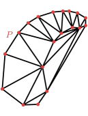
Figure 1: A planar point set $\color[rgb]{0.75,0.30,0.15}P$, and a quadtree (a) and a Delaunay triangulation (b) on it.

Delaunay triangulations and quadtrees are among the oldest and best-studied notions in computational geometry [3, 6, 24, 28, 42, 45, 47, 43], captivating the attention of researchers for almost four decades. Both are proximity structures on planar point sets; Figure 1 shows a simple example of these structures. Here, we will demonstrate that they are, in fact, equivalent in a very strong sense. Specifically, we describe two algorithms. The first computes a suitable quadtree for $\color[rgb]{0.75,0.30,0.15}P$, given the Delaunay triangulation $\color[rgb]{0.75,0.30,0.15}\operatorname{DT}(P)$. This algorithm closely follows a previous result by Krznaric and Levcopolous [38], who solve this problem in a stronger model of computation. Our contribution lies in adapting their algorithm to the real RAM/pointer machine model. The second algorithm, which is the main focus of this paper, goes in the other direction and computes $\color[rgb]{0.75,0.30,0.15}\operatorname{DT}(P)$, assuming that a suitable quadtree for $\color[rgb]{0.75,0.30,0.15}P$ is at hand.

The connection between quadtrees and Delaunay triangulations was first discovered and fruitfully applied by Buchin and Mulzer [9] (see also [8]). While their approach is to use a hierarchy of quadtrees for faster conflict location in a randomized incremental construction of $\color[rgb]{0.75,0.30,0.15}\operatorname{DT}(P)$, we pursue a strategy similar to the one by Löffler and Snoeyink [40]: we use the additional information to find a connected subgraph of $\color[rgb]{0.75,0.30,0.15}\operatorname{DT}(P)$, from which $\color[rgb]{0.75,0.30,0.15}\operatorname{DT}(P)$ can be computed in linear deterministic time [20]. As in Löffler and Snoeyink [40], our subgraph of choice is the Euclidean minimum spanning tree (EMST) for $\color[rgb]{0.75,0.30,0.15}P$, $\color[rgb]{0.75,0.30,0.15}\operatorname{emst}(P)$ [26]. The connection between quadtrees and EMSTs is well known: initially, quadtrees were used to obtain fast approximations to $\color[rgb]{0.75,0.30,0.15}\operatorname{emst}(P)$ in high dimensions [11, 49]. Developing these ideas further, several algorithms were found that use the well-separated pair decomposition (WSPD) [12], or a variant thereof, to reduce EMST computation to solving the bichromatic closest pair problem. In that problem, we are given two point sets $\color[rgb]{0.75,0.30,0.15}R$ and $\color[rgb]{0.75,0.30,0.15}B$, and we look for a pair $\color[rgb]{0.75,0.30,0.15}(r,b)\in R\times B$ that minimizes the distance $\color[rgb]{0.75,0.30,0.15}|rb|$ [1, 11, 39, 51]. Given a quadtree for $\color[rgb]{0.75,0.30,0.15}P$, a WSPD for $\color[rgb]{0.75,0.30,0.15}P$ can be found in linear time [8, 12, 13, 33]. EMST algorithms based on bichromatic closest pairs constitute the fastest known solutions in higher dimensions. Our approach is quite similar, but we focus exclusively on the plane. We use the quadtree and WSPDs to obtain a sequence of bichromatic closest pair problems, which then yield a sparse supergraph of the EMST. There are several issues: we need to ensure that the bichromatic closest pair problems have total linear size and can be solved in linear time, and we also need to extract the EMST from the supergraph in linear time. In this paper we show how to do this using the structure of the quadtree, combined with a partition of the point set according to angular segments similar to Yao’s technique [51].

1.1 Applications

Our two algorithms have several implications for derandomizing recent algorithms related to DTs. First, we mention hereditary computation of DTs. Chazelle et al. [18] show how to split a Delaunay triangulation in linear expected time (see also [19]). That is, given $\color[rgb]{0.75,0.30,0.15}\operatorname{DT}(P\cup Q)$, they describe a randomized algorithm to find $\color[rgb]{0.75,0.30,0.15}\operatorname{DT}(P)$ and $\color[rgb]{0.75,0.30,0.15}\operatorname{DT}(Q)$ in expected time $\color[rgb]{0.75,0.30,0.15}O(|P|+|Q|)$. Knowing that DTs and quadtrees are equivalent, this result becomes almost obvious, as quadtrees are easily split in linear time. More importantly, our new algorithm achieves linear worst-case running time. Ailon et al. [2] use hereditary DTs for self-improving algorithms [2]. Together with the $\color[rgb]{0.75,0.30,0.15}\varepsilon$-net construction by Pyrga and Ray [44] (see [2, Appendix A]), our result yields a deterministic version of their algorithm for point sets generated by a random source (the inputs are probabilistic, but not the algorithm).

Eppstein et al. [27] introduce the skip-quadtree and show how to turn a (compressed) quadtree into a skip-quadtree in linear time. Buchin and Mulzer [9] use a (randomized) skip-quadtree to find the DT in linear expected time. This yields several improved results about computing DTs. Most notably, they show that in the transdichotomous setting [15, 14, 29], computing DTs is no harder than sorting the points (according to some special order). Here, we show how to go directly from a quadtree to a DT, without skip-quadtrees or randomness. This gives the first deterministic transdichotomous reduction from DTs to sorting.

Buchin et al. [8] use both hereditary DTs and the connection between skip-quadtrees and DTs to simplify and generalize an algorithm by Löffler and Snoeyink [40] to preprocess imprecise points for Delaunay triangulation in linear expected time (see also Devillers [25] for another simplified, but not worst-case optimal, solution). Löffler and Snoeyink’s original algorithm is deterministic, and the derandomized version of the Buchin et al. algorithm proceeds in a very similar spirit. However, we now have an optimal deterministic solution for the generalized problem as well.

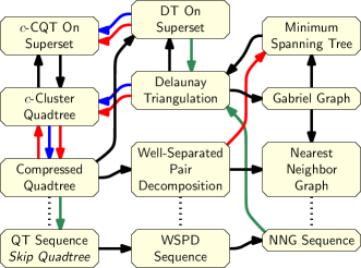
Figure 2: We show which can be computed from which in linear time. The black arrows depict known linear time deterministic algorithms that work in the pointer machine/real RAM model. The red arrows depict our new results. Furthermore, for reference, we also show known randomized linear time algorithms (in green) and known deterministic linear time algorithms that work in a weaker model of computation (in blue).

In Figure 2, we show a graphical representation of different proximity structures on planar point sets. The arrows show which structures can be computed from which in linear deterministic time on a pointer machine, before and after this paper. Please realize that there are several subtleties of different algorithms and their interactions that are hard to show in a diagram, it is included purely as illustration of the impact of our results.

1.2 Organization of this paper

The main result of our paper is an algorithm to compute a minimum spanning tree of a set of points from a given compressed quadtree. However, before we can describe this result in Section 4, we need to establish the necessary tools; to this end we review several known concepts in Section 2 and prove some related technical lemmas in Section 3. In Section 5, we describe the algorithm to compute a quadtree when given the Delaunay triangulation; this is an adaptation of the algorithm by Krznaric and Levcopoulos [38] to the real RAM model. Finally, we detail some important implications of our two new algorithms in Section 6.

2 Preliminaries

We review some known definitions, structures, algorithms, and their relationships.

2.1 Delaunay Triangulations and Euclidean Minimum Spanning Trees

Given a set $\color[rgb]{0.75,0.30,0.15}P$ of $\color[rgb]{0.75,0.30,0.15}n$ points in the plane, an important and extensively studied structure is the Delaunay triangulation of $\color[rgb]{0.75,0.30,0.15}P$ [3, 6, 24, 43, 47], denoted $\color[rgb]{0.75,0.30,0.15}\operatorname{DT}(P)$. It can be defined as the dual graph of the Voronoi diagram, the triangulation that optimizes the smallest angle in any triangle, or in many other equivalent ways, and it has been proven to optimize many other different criteria [42].

The Euclidean minimum spanning tree of $\color[rgb]{0.75,0.30,0.15}P$, denoted $\color[rgb]{0.75,0.30,0.15}\operatorname{emst}(P)$, is the tree of smallest total edge length that has the points of $\color[rgb]{0.75,0.30,0.15}P$ as its vertices, and it is well known that the EMST is a subgraph of the DT [47, Theorem 7]. In the following, we will assume that all the pairwise distances in $\color[rgb]{0.75,0.30,0.15}P$ are distinct (a general position assumption), which implies that $\color[rgb]{0.75,0.30,0.15}\operatorname{emst}(P)$ is uniquely determined. Finally, we remind the reader that $\color[rgb]{0.75,0.30,0.15}\operatorname{emst}(P)$, like every minimum spanning tree, has the following cut property: let $\color[rgb]{0.75,0.30,0.15}P=R\cup B$ a partition of $\color[rgb]{0.75,0.30,0.15}P$, and let $\color[rgb]{0.75,0.30,0.15}r$ and $\color[rgb]{0.75,0.30,0.15}b$ be the two points with $\color[rgb]{0.75,0.30,0.15}r\in R$ and $\color[rgb]{0.75,0.30,0.15}b\in B$ that minimize the distance $\color[rgb]{0.75,0.30,0.15}|rb|$. Then $\color[rgb]{0.75,0.30,0.15}rb$ is an edge of $\color[rgb]{0.75,0.30,0.15}\operatorname{emst}(P)$. Note that this is very similar to the bichromatic closest pair reduction mentioned in the introduction, but the cut property holds for any partition of $\color[rgb]{0.75,0.30,0.15}P$, whereas the bichromatic closest pair reduction requires a very specific decomposition of $\color[rgb]{0.75,0.30,0.15}P$ into pairs of subsets (which is usually not a partition).

2.2 Quadtrees—Compressed and $\color[rgb]{0.75,0.30,0.15}c$-Cluster

Let $\color[rgb]{0.75,0.30,0.15}P$ be a planar point set. The spread of $\color[rgb]{0.75,0.30,0.15}P$ is defined as the ratio between the largest and the smallst distance between any two distinct points in $\color[rgb]{0.75,0.30,0.15}P$. A quadtree for $\color[rgb]{0.75,0.30,0.15}P$ is a hierarchical decomposition of an axis-aligned bounding square for $\color[rgb]{0.75,0.30,0.15}P$ into smaller axis-aligned squares [3, 28, 33, 45]. A regular quadtree is constructed by successively subdividing every square with at least two points into four congruent child squares. A node $\color[rgb]{0.75,0.30,0.15}v$ of a quadtree is associated with (i) $\color[rgb]{0.75,0.30,0.15}S_{v}$, the square corresponding to $\color[rgb]{0.75,0.30,0.15}v$; (ii) $\color[rgb]{0.75,0.30,0.15}P_{v}$, the points contained in $\color[rgb]{0.75,0.30,0.15}S_{v}$; and (iii) $\color[rgb]{0.75,0.30,0.15}B_{v}$, the axis-aligned bounding square for $\color[rgb]{0.75,0.30,0.15}P_{v}$. $\color[rgb]{0.75,0.30,0.15}S_{v}$ and $\color[rgb]{0.75,0.30,0.15}B_{v}$ are stored explicitly at the node. We write $\color[rgb]{0.75,0.30,0.15}|S_{v}|$ and $\color[rgb]{0.75,0.30,0.15}|B_{v}|$ for the diameter of $\color[rgb]{0.75,0.30,0.15}S_{v}$ and $\color[rgb]{0.75,0.30,0.15}B_{v}$, and $\color[rgb]{0.75,0.30,0.15}c_{v}$ for the center of $\color[rgb]{0.75,0.30,0.15}S_{v}$. We will also use the shorthand $\color[rgb]{0.75,0.30,0.15}d(u,v):=d(S_{u},S_{v})$ to denote the shortest distance between any point in $\color[rgb]{0.75,0.30,0.15}S_{u}$ and any point in $\color[rgb]{0.75,0.30,0.15}S_{v}$. Furthermore, we denote the parent of $\color[rgb]{0.75,0.30,0.15}v$ by $\color[rgb]{0.75,0.30,0.15}\overline{v}$. Regular quadtrees can have unbounded depth (if $\color[rgb]{0.75,0.30,0.15}P$ has unbounded spread so in order to give any theoretical guarantees the concept is usually refined. In the sequel, we use two such variants of quadtrees, namely compressed and $\color[rgb]{0.75,0.30,0.15}c$-cluster quadtrees, which we show are in fact equivalent.

A compressed quadtree is a quadtree in which we replace long paths of nodes with only one child by a single edge [4, 5, 8, 21]. It has size $\color[rgb]{0.75,0.30,0.15}O(|P|)$. Formally, given a large constant $\color[rgb]{0.75,0.30,0.15}a$, an $\color[rgb]{0.75,0.30,0.15}a$-compressed quadtree is a regular quadtree with additional compressed nodes. A compressed node $\color[rgb]{0.75,0.30,0.15}v$ has only one child $\color[rgb]{0.75,0.30,0.15}\underline{v}$ with $\color[rgb]{0.75,0.30,0.15}|S_{\underline{v}}|\leq|S_{v}|/a$ and such that $\color[rgb]{0.75,0.30,0.15}S_{v}\setminus S_{\underline{v}}$ has no points from $\color[rgb]{0.75,0.30,0.15}P$. Figure 3 shows an example. Note that in our definition $\color[rgb]{0.75,0.30,0.15}S_{\underline{v}}$ need not be aligned with $\color[rgb]{0.75,0.30,0.15}S_{v}$, which would happen if we literally “compressed” a regular quadtree. This relaxed definition is necessary because existing algorithms for computing aligned compressed quadtrees use a more powerful model of computation than our real RAM/pointer machine (see Appendix A). In the usual applications of quadtrees, this is acceptable. In fact, Har-Peled [33, Chapter 2] pointed out that some non-standard operation is inevitable if we require that the squares of the compressed quadtree are perfectly aligned. However, here we intend to derandomize algorithms that work on a traditional real RAM/pointer machine, so we prefer to stay in this model. This keeps our results comparable with the previous work.

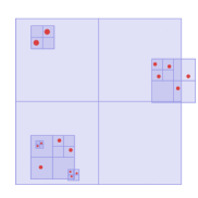
Figure 3: (a) A compressed quadtree on a set of $\color[rgb]{0.75,0.30,0.15}15$ points. (b) A $\color[rgb]{0.75,0.30,0.15}c$-cluster tree on the same point set. (c) In a $\color[rgb]{0.75,0.30,0.15}c$-cluster quadtree, the internal nodes of the $\color[rgb]{0.75,0.30,0.15}c$-cluster tree are replaced by quadtrees.

Now let $\color[rgb]{0.75,0.30,0.15}c$ be a large enough constant. A subset $\color[rgb]{0.75,0.30,0.15}U\subseteq P$ is a $\color[rgb]{0.75,0.30,0.15}c$-cluster if $\color[rgb]{0.75,0.30,0.15}U=P$ or $\color[rgb]{0.75,0.30,0.15}d(U,P\setminus U)\geq c|B_{U}|$, where $\color[rgb]{0.75,0.30,0.15}B_{U}$ denotes the smallest axis-aligned bounding square for $\color[rgb]{0.75,0.30,0.15}U$, and $\color[rgb]{0.75,0.30,0.15}d(A,B)$ is the minimum distance between a point in $\color[rgb]{0.75,0.30,0.15}A$ and a point in $\color[rgb]{0.75,0.30,0.15}B$ [37, 38]. In other words, $\color[rgb]{0.75,0.30,0.15}U$ is a $\color[rgb]{0.75,0.30,0.15}c$-cluster precisely if $\color[rgb]{0.75,0.30,0.15}\{U,P\setminus U\}$ is a $\color[rgb]{0.75,0.30,0.15}(1/c)$-semi-separated pair [33, 50]. It is easily seen that the $\color[rgb]{0.75,0.30,0.15}c$-clusters for $\color[rgb]{0.75,0.30,0.15}P$ form a laminar family, i.e., a set system in which any two sets $\color[rgb]{0.75,0.30,0.15}A$ and $\color[rgb]{0.75,0.30,0.15}B$ satisfy either $\color[rgb]{0.75,0.30,0.15}A\cap B=\emptyset$; $\color[rgb]{0.75,0.30,0.15}A\subseteq B$; or $\color[rgb]{0.75,0.30,0.15}B\subseteq A$. Thus, the $\color[rgb]{0.75,0.30,0.15}c$-clusters define a $\color[rgb]{0.75,0.30,0.15}c$-cluster tree $\color[rgb]{0.75,0.30,0.15}T_{c}$. Figure 3 shows an example. These trees are a very natural way to tackle point sets of unbounded spread, and they have linear size. However, they also may have high degree. To avoid this, a $\color[rgb]{0.75,0.30,0.15}c$-cluster tree $\color[rgb]{0.75,0.30,0.15}T_{c}$ can be augmented by additional nodes, adding more structure to the parts of the point set that are not strongly clustered. This is done as follows. First, recall that a quadtree is called balanced if for every node $\color[rgb]{0.75,0.30,0.15}u$ that is either a leaf or a compressed node, the square $\color[rgb]{0.75,0.30,0.15}S_{u}$ is adjacent only to squares that are within a factor $\color[rgb]{0.75,0.30,0.15}2$ of the size of $\color[rgb]{0.75,0.30,0.15}S_{u}$. For each internal node $\color[rgb]{0.75,0.30,0.15}u$ of $\color[rgb]{0.75,0.30,0.15}T_{c}$ with set of children $\color[rgb]{0.75,0.30,0.15}V$, we build a balanced regular quadtree on a set of points containing one representative point from each node in $\color[rgb]{0.75,0.30,0.15}V$ (the intuition being that such a cluster is so small and far from its neighbors, that we might as well treat it as a point). This quadtree has size $\color[rgb]{0.75,0.30,0.15}O(|V|)$ (Lemma 3.4), so we obtain a tree of constant degree and linear size, the $\color[rgb]{0.75,0.30,0.15}c$-cluster quadtree. Figure 3 shows an example. The sets $\color[rgb]{0.75,0.30,0.15}P_{v}$, $\color[rgb]{0.75,0.30,0.15}S_{v}$ and $\color[rgb]{0.75,0.30,0.15}B_{v}$ for the $\color[rgb]{0.75,0.30,0.15}c$-cluster quadtree are just as for regular and compressed quadtrees, where in $\color[rgb]{0.75,0.30,0.15}P_{v}$ we expand the representative points appropriately. Note that it is possible that $\color[rgb]{0.75,0.30,0.15}S_{v}\nsupseteq P_{v}$, but the points of $\color[rgb]{0.75,0.30,0.15}P_{v}$ can never be too far from $\color[rgb]{0.75,0.30,0.15}S_{v}$. In Section 3.1 we elaborate more on $\color[rgb]{0.75,0.30,0.15}c$-cluster quadtrees and their properties, and in Section 3.3, we prove that $\color[rgb]{0.75,0.30,0.15}c$-cluster quadtrees and compressed quadtrees are equivalent (Theorem 3.12).

2.3 Well-Separated Pair Decompositions

For any two finite sets $\color[rgb]{0.75,0.30,0.15}U$ and $\color[rgb]{0.75,0.30,0.15}V$, let $\color[rgb]{0.75,0.30,0.15}U\otimes V:=\{\{u,v\}\mid u\in U,v\in V,u\neq v\}$. A pair decomposition $\color[rgb]{0.75,0.30,0.15}\mathcal{P}$ for a planar $\color[rgb]{0.75,0.30,0.15}n$-point set $\color[rgb]{0.75,0.30,0.15}P$ is a set of $\color[rgb]{0.75,0.30,0.15}m$ pairs $\color[rgb]{0.75,0.30,0.15}\{\{U_{1},V_{1}\},$ $\color[rgb]{0.75,0.30,0.15}\ldots,$ $\color[rgb]{0.75,0.30,0.15}\{U_{m},V_{m}\}\}$, such that (i) for all $\color[rgb]{0.75,0.30,0.15}i=1,\ldots,m$, we have $\color[rgb]{0.75,0.30,0.15}U_{i},V_{i}\subseteq P$ and $\color[rgb]{0.75,0.30,0.15}U_{i}\cap V_{i}=\emptyset$; and (ii) for any $\color[rgb]{0.75,0.30,0.15}\{p,q\}\in P\otimes P$, there is exactly one $\color[rgb]{0.75,0.30,0.15}i$ with $\color[rgb]{0.75,0.30,0.15}\{p,q\}\in U_{i}\otimes V_{i}$. We call $\color[rgb]{0.75,0.30,0.15}m$ the size of $\color[rgb]{0.75,0.30,0.15}\mathcal{P}$. Fix a constant $\color[rgb]{0.75,0.30,0.15}\varepsilon\in(0,1)$, and let $\color[rgb]{0.75,0.30,0.15}\{U,V\}\in\mathcal{P}$. Denote by $\color[rgb]{0.75,0.30,0.15}B_{U}$, $\color[rgb]{0.75,0.30,0.15}B_{V}$ the smallest axis-aligned squares containing $\color[rgb]{0.75,0.30,0.15}U$ and $\color[rgb]{0.75,0.30,0.15}V$. We say that $\color[rgb]{0.75,0.30,0.15}\{U,V\}$ is $\color[rgb]{0.75,0.30,0.15}\varepsilon$-well-separated if $\color[rgb]{0.75,0.30,0.15}\max\{|B_{U}|,|B_{V}|\}\leq\varepsilon d(B_{U},B_{V})$, where $\color[rgb]{0.75,0.30,0.15}d(B_{U},B_{V})$ is the distance between $\color[rgb]{0.75,0.30,0.15}B_{U}$ and $\color[rgb]{0.75,0.30,0.15}B_{V}$ (i.e., the smallest distance between a point in $\color[rgb]{0.75,0.30,0.15}B_{U}$ and a point in $\color[rgb]{0.75,0.30,0.15}B_{V}$). If $\color[rgb]{0.75,0.30,0.15}\{U,V\}$ is not $\color[rgb]{0.75,0.30,0.15}\varepsilon$-well-separated, we say it is $\color[rgb]{0.75,0.30,0.15}\varepsilon$-ill-separated. We call $\color[rgb]{0.75,0.30,0.15}\mathcal{P}$ an $\color[rgb]{0.75,0.30,0.15}\varepsilon$-well-separated pair decomposition ($\color[rgb]{0.75,0.30,0.15}\varepsilon$-WSPD) if all its pairs are $\color[rgb]{0.75,0.30,0.15}\varepsilon$-well-separated [11, 12, 26, 33].

Now let $\color[rgb]{0.75,0.30,0.15}T$ be a (compressed or $\color[rgb]{0.75,0.30,0.15}c$-cluster) quadtree for $\color[rgb]{0.75,0.30,0.15}P$. Given $\color[rgb]{0.75,0.30,0.15}\varepsilon>0$, it is well known that $\color[rgb]{0.75,0.30,0.15}T$ can be used to obtain an $\color[rgb]{0.75,0.30,0.15}\varepsilon$-WSPD for $\color[rgb]{0.75,0.30,0.15}P$ in linear time [12, 33]. Since we will need some specific properties of such an $\color[rgb]{0.75,0.30,0.15}\varepsilon$-WSPD, we give pseudo-code for such an algorithm in Algorithm 1. We call this algorithm $\color[rgb]{0.75,0.30,0.15}\operatorname{\texttt{wspd}}$, and denote its output on input $\color[rgb]{0.75,0.30,0.15}T$ by $\color[rgb]{0.75,0.30,0.15}\operatorname{\texttt{wspd}}(T)$. The correctness of the algorithm $\color[rgb]{0.75,0.30,0.15}\operatorname{\texttt{wspd}}$ is immediate, since it only outputs well-separated pairs, and the bounds on the running time and the size of $\color[rgb]{0.75,0.30,0.15}\operatorname{\texttt{wspd}}(T)$ follow from a well-known volume argument which we omit [8, 12, 13, 33].

1. Call $\color[rgb]{0.75,0.30,0.15}\operatorname{\texttt{wspd}}(r)$ on the root $\color[rgb]{0.75,0.30,0.15}r$ of $\color[rgb]{0.75,0.30,0.15}T$.

$\color[rgb]{0.75,0.30,0.15}\operatorname{\texttt{wspd}}(v)$

1. If $\color[rgb]{0.75,0.30,0.15}v$ is a leaf, return $\color[rgb]{0.75,0.30,0.15}\emptyset$.

2. Return the union of $\color[rgb]{0.75,0.30,0.15}\operatorname{\texttt{wspd}}(w)$ and $\color[rgb]{0.75,0.30,0.15}\operatorname{\texttt{wspd}}(\{w_{1},w_{2}\})$ for all children $\color[rgb]{0.75,0.30,0.15}w$ and pairs of distinct children $\color[rgb]{0.75,0.30,0.15}w_{1},w_{2}$ of $\color[rgb]{0.75,0.30,0.15}v$.

$\color[rgb]{0.75,0.30,0.15}\operatorname{\texttt{wspd}}(\{u,v\})$

1. If $\color[rgb]{0.75,0.30,0.15}S_{u}$ and $\color[rgb]{0.75,0.30,0.15}S_{v}$ are $\color[rgb]{0.75,0.30,0.15}\varepsilon$-well-separated, return $\color[rgb]{0.75,0.30,0.15}\{u,v\}$.

2. Otherwise, if $\color[rgb]{0.75,0.30,0.15}|S_{u}|\leq|S_{v}|$, return the union of $\color[rgb]{0.75,0.30,0.15}\operatorname{\texttt{wspd}}(\{u,w\})$ for all children $\color[rgb]{0.75,0.30,0.15}w$ of $\color[rgb]{0.75,0.30,0.15}v$.

3. Otherwise, return the union of $\color[rgb]{0.75,0.30,0.15}\operatorname{\texttt{wspd}}(\{w,v\})$ for all children $\color[rgb]{0.75,0.30,0.15}w$ of $\color[rgb]{0.75,0.30,0.15}u$.

Algorithm 1 Finding a well-separated pair decomposition.

Theorem 2.1.

There is an algorithm $\color[rgb]{0.75,0.30,0.15}\operatorname{\texttt{wspd}}$, that given a (compressed or $\color[rgb]{0.75,0.30,0.15}c$-cluster) quadtree $\color[rgb]{0.75,0.30,0.15}T$ for a planar $\color[rgb]{0.75,0.30,0.15}n$-point set $\color[rgb]{0.75,0.30,0.15}P$, finds in time $\color[rgb]{0.75,0.30,0.15}O(n)$ a linear-size $\color[rgb]{0.75,0.30,0.15}\varepsilon$-WSPD for $\color[rgb]{0.75,0.30,0.15}P$, denoted $\color[rgb]{0.75,0.30,0.15}\operatorname{\texttt{wspd}}(T)$. ∎

Note that the WSPD is not stored explicitly: we cannot afford to store all the pairs $\color[rgb]{0.75,0.30,0.15}\{U,V\}$, since their total size might be quadratic. Instead, $\color[rgb]{0.75,0.30,0.15}\operatorname{\texttt{wspd}}(T)$ contains pairs $\color[rgb]{0.75,0.30,0.15}\{u,v\}$, where $\color[rgb]{0.75,0.30,0.15}u$ and $\color[rgb]{0.75,0.30,0.15}v$ are nodes in $\color[rgb]{0.75,0.30,0.15}T$, and $\color[rgb]{0.75,0.30,0.15}\{u,v\}$ is used to represent the pair $\color[rgb]{0.75,0.30,0.15}\{P_{u},P_{v}\}$.

Note that the algorithm computes the WSPD with respect to the squares $\color[rgb]{0.75,0.30,0.15}S_{v}$, instead of the bounding squares $\color[rgb]{0.75,0.30,0.15}B_{v}$. This makes no big difference, since for compressed quadtrees $\color[rgb]{0.75,0.30,0.15}B_{v}\subseteq S_{v}$, and for $\color[rgb]{0.75,0.30,0.15}c$-cluster quadtrees $\color[rgb]{0.75,0.30,0.15}B_{v}$ can be outside $\color[rgb]{0.75,0.30,0.15}S_{v}$ only for $\color[rgb]{0.75,0.30,0.15}c$-cluster nodes, resulting in a loss of at most a factor $\color[rgb]{0.75,0.30,0.15}1+1/c$ in separation. Referring to the pseudo-code in Algorithm 1, we now prove three observations. The first observation says that the size of the squares under consideration strictly decreases throughout the algorithm.

Observation 2.2.

Let $\color[rgb]{0.75,0.30,0.15}\{u,v\}$ be a pair of distinct nodes of $\color[rgb]{0.75,0.30,0.15}T$. If $\color[rgb]{0.75,0.30,0.15}\operatorname{\texttt{wspd}}(\{u,v\})$ is executed by $\color[rgb]{0.75,0.30,0.15}\operatorname{\texttt{wspd}}$ run on $\color[rgb]{0.75,0.30,0.15}T$ (in particular, if $\color[rgb]{0.75,0.30,0.15}\{u,v\}\in\operatorname{\texttt{wspd}}(T)$), then $\color[rgb]{0.75,0.30,0.15}\max\{|S_{u}|,|S_{v}|\}\leq\min\{|S_{\overline{u}}|,|S_{\overline{v}}|\}$.

Proof.

We use induction on the depth of the call stack for $\color[rgb]{0.75,0.30,0.15}\operatorname{\texttt{wspd}}(\{u,v\})$. Initially, $\color[rgb]{0.75,0.30,0.15}u$ and $\color[rgb]{0.75,0.30,0.15}v$ are children of the same node, and the statement holds. Furthermore, assuming that $\color[rgb]{0.75,0.30,0.15}\operatorname{\texttt{wspd}}(\{u,v\})$ is called by $\color[rgb]{0.75,0.30,0.15}\operatorname{\texttt{wspd}}(\{u,\overline{v}\})$ (and hence $\color[rgb]{0.75,0.30,0.15}|S_{u}|\leq|S_{\overline{v}}|$), we get $\color[rgb]{0.75,0.30,0.15}\max\{|S_{u}|,|S_{v}|\}\leq|S_{\overline{v}}|=\min\{|S_{\overline{u}}|,|S_{\overline{v}}|\}$, where the last equation follows by induction. ∎

The next observation states that the wspd-pairs reported by the algorithm are, in a sense, as high in the tree as possible.

Observation 2.3.

If $\color[rgb]{0.75,0.30,0.15}\{u,v\}\in\operatorname{\texttt{wspd}}(T)$, then $\color[rgb]{0.75,0.30,0.15}\overline{u}$ and $\color[rgb]{0.75,0.30,0.15}\overline{v}$ are ill-separated.

Proof.

If $\color[rgb]{0.75,0.30,0.15}\overline{u}=\overline{v}$, the claim is obvious. Otherwise, let us assume that $\color[rgb]{0.75,0.30,0.15}\operatorname{\texttt{wspd}}(\{u,v\})$ was called by $\color[rgb]{0.75,0.30,0.15}\operatorname{\texttt{wspd}}(\{u,\overline{v}\})$. This means that $\color[rgb]{0.75,0.30,0.15}\{u,\overline{v}\}$ is ill-separated and $\color[rgb]{0.75,0.30,0.15}\max\{|S_{u}|,|S_{\overline{v}}|\}=|S_{\overline{v}}|$. Therefore, $\color[rgb]{0.75,0.30,0.15}\max\{|S_{\overline{u}}|,|S_{\overline{v}}|\}\geq|S_{\overline{v}}|>\varepsilon d(u,\overline{v})\geq\varepsilon d(\overline{u},\overline{v})$, and $\color[rgb]{0.75,0.30,0.15}\{\overline{u},\overline{v}\}$ is ill-separated. ∎

The last claim shows that for each wspd-pair, we can find well-behaved boxes whose size is comparable to the distance between the point sets. In the following, this will be a useful tool for making volume arguments that bound the number of wspd-pairs to consider.

Claim 2.4.

Let $\color[rgb]{0.75,0.30,0.15}\{u,v\}\in\operatorname{\texttt{wspd}}(T)$. Then there exist squares $\color[rgb]{0.75,0.30,0.15}R_{u}$ and $\color[rgb]{0.75,0.30,0.15}R_{v}$ such that (i) $\color[rgb]{0.75,0.30,0.15}S_{u}\subseteq R_{u}\subseteq S_{\overline{u}}$ and $\color[rgb]{0.75,0.30,0.15}S_{v}\subseteq R_{v}\subseteq S_{\overline{v}}$; (ii) $\color[rgb]{0.75,0.30,0.15}|R_{u}|=|R_{v}|$; and (iii) $\color[rgb]{0.75,0.30,0.15}|R_{u}|/2\varepsilon\leq d(R_{u},R_{v})\leq 2|R_{u}|/\varepsilon$.

Proof.

Suppose $\color[rgb]{0.75,0.30,0.15}\operatorname{\texttt{wspd}}(\{u,v\})$ is called by $\color[rgb]{0.75,0.30,0.15}\operatorname{\texttt{wspd}}(\{u,\overline{v}\})$, the other case is symmetric. Let us define $\color[rgb]{0.75,0.30,0.15}r:=\min\{\varepsilon d(u,v),|S_{\overline{v}}|\}$. By Observation 2.2, we have $\color[rgb]{0.75,0.30,0.15}|S_{u}|,|S_{v}|\leq|S_{\overline{v}}|\leq|S_{\overline{u}}|$. Since $\color[rgb]{0.75,0.30,0.15}\{u,v\}$ is well-separated, we have $\color[rgb]{0.75,0.30,0.15}\varepsilon d(u,v)\geq\max\{|S_{u}|,|S_{v}|\}$. Hence, $\color[rgb]{0.75,0.30,0.15}|S_{\overline{u}}|,|S_{\overline{v}}|\geq r\geq|S_{u}|,|S_{v}|$, and we can pick squares $\color[rgb]{0.75,0.30,0.15}R_{u}$ and $\color[rgb]{0.75,0.30,0.15}R_{v}$ of diameter $\color[rgb]{0.75,0.30,0.15}r$ that fulfill (i). Now (ii) holds by construction, and it remains to check (iii). First, note that $\color[rgb]{0.75,0.30,0.15}d(R_{u},R_{v})\geq d(u,v)-2r\geq(1-2\varepsilon)d(u,v)\geq r/2\varepsilon$, for $\color[rgb]{0.75,0.30,0.15}\varepsilon\leq 1/4$. This proves the lower bound. For the upper bound, observe that $\color[rgb]{0.75,0.30,0.15}\varepsilon d(u,v)\leq\varepsilon(d(u,\overline{v})+|S_{\overline{v}}|)\leq(1+\varepsilon)|S_{\overline{v}}|$, because $\color[rgb]{0.75,0.30,0.15}\{u,\overline{v}\}$ is ill-separated. Thus, we have $\color[rgb]{0.75,0.30,0.15}\varepsilon d(u,v)/2\leq r$, and $\color[rgb]{0.75,0.30,0.15}d(R_{u},R_{v})\leq d(u,v)\leq 2r/\varepsilon$, as desired. ∎

3 More on Quadtrees

In this section, we describe a few more properties of the $\color[rgb]{0.75,0.30,0.15}c$-cluster trees and $\color[rgb]{0.75,0.30,0.15}c$-cluster quadtrees defined in Section 2.2, and we prove that they are equivalent to the more standard compressed quadtrees (Theorem 3.12). Since most of the material is very technical, we encourage the impatient reader to skip ahead to Section 4.

3.1 $\color[rgb]{0.75,0.30,0.15}c$-Cluster Quadtrees

Krznaric and Levcopolous [37, Theorem 7] showed that a $\color[rgb]{0.75,0.30,0.15}c$-cluster tree can be computed in linear time from a Delaunay triangulation.

Theorem 3.1 (Krznaric-Levcopolous).

Let $\color[rgb]{0.75,0.30,0.15}P$ be a planar $\color[rgb]{0.75,0.30,0.15}n$-point set. Given a constant $\color[rgb]{0.75,0.30,0.15}c\geq 1$ and $\color[rgb]{0.75,0.30,0.15}\operatorname{DT}(P)$, we can find a $\color[rgb]{0.75,0.30,0.15}c$-cluster tree $\color[rgb]{0.75,0.30,0.15}T_{c}$ for $\color[rgb]{0.75,0.30,0.15}P$ in $\color[rgb]{0.75,0.30,0.15}O(n)$ time and space on a pointer machine. ∎

Here, we will actually use a more relaxed notion of $\color[rgb]{0.75,0.30,0.15}c$-cluster trees: let $\color[rgb]{0.75,0.30,0.15}c_{1}$, $\color[rgb]{0.75,0.30,0.15}c_{2}$ be two constants with $\color[rgb]{0.75,0.30,0.15}1\leq c_{1}\leq c_{2}$, and let $\color[rgb]{0.75,0.30,0.15}P$ be a planar $\color[rgb]{0.75,0.30,0.15}n$-point set. A $\color[rgb]{0.75,0.30,0.15}(c_{1},c_{2})$-cluster tree $\color[rgb]{0.75,0.30,0.15}T_{(c_{1},c_{2})}$ is a rooted tree in which each inner node has at least two children and which has $\color[rgb]{0.75,0.30,0.15}n$ leaves, one for each point in $\color[rgb]{0.75,0.30,0.15}P$. Each node $\color[rgb]{0.75,0.30,0.15}v\in T_{(c_{1},c_{2})}$ corresponds to a subset $\color[rgb]{0.75,0.30,0.15}P_{v}\subseteq P$ in the natural way. Every node $\color[rgb]{0.75,0.30,0.15}v$ must fulfill two properties: (i) if $\color[rgb]{0.75,0.30,0.15}v$ is not the root, then $\color[rgb]{0.75,0.30,0.15}d(P_{v},P\setminus P_{v})\geq c_{1}|B_{P_{v}}|$; and (ii) if $\color[rgb]{0.75,0.30,0.15}P_{v}$ has a proper subset $\color[rgb]{0.75,0.30,0.15}Q\subset P_{v}$ with $\color[rgb]{0.75,0.30,0.15}d(Q,P\setminus Q)\geq c_{2}|B_{Q}|$, then there is a child $\color[rgb]{0.75,0.30,0.15}w$ of $\color[rgb]{0.75,0.30,0.15}v$ with $\color[rgb]{0.75,0.30,0.15}Q\subseteq P_{w}$. In other words, each node of $\color[rgb]{0.75,0.30,0.15}T_{(c_{1},c_{2})}$ corresponds to a $\color[rgb]{0.75,0.30,0.15}c_{1}$-cluster of $\color[rgb]{0.75,0.30,0.15}P$, and $\color[rgb]{0.75,0.30,0.15}T_{(c_{1},c_{2})}$ must have a node for every $\color[rgb]{0.75,0.30,0.15}c_{2}$-cluster of $\color[rgb]{0.75,0.30,0.15}P$. Thus, the original $\color[rgb]{0.75,0.30,0.15}c$-cluster tree is also a $\color[rgb]{0.75,0.30,0.15}(c,c)$-cluster tree. Our relaxed definition allows for some flexibility in the construction of $\color[rgb]{0.75,0.30,0.15}T_{(c_{1},c_{2})}$ while providing the same benefits as the original $\color[rgb]{0.75,0.30,0.15}c$-cluster tree. Thus, outside this section we will be slightly sloppy and not distinguish between $\color[rgb]{0.75,0.30,0.15}c$-cluster trees and $\color[rgb]{0.75,0.30,0.15}(c,\Theta(c))$-cluster trees.

As mentioned above, the tree $\color[rgb]{0.75,0.30,0.15}T_{(c_{1},c_{2})}$ is quite similar to a well-separated pair decomposition: any two unrelated nodes in $\color[rgb]{0.75,0.30,0.15}T_{(c_{1},c_{2})}$ correspond to a $\color[rgb]{0.75,0.30,0.15}(1/c_{1})$-well-separated pair. However, $\color[rgb]{0.75,0.30,0.15}T_{(c_{1},c_{2})}$ has the huge drawback that it may contain nodes of unbounded degree. For example, if the points in $\color[rgb]{0.75,0.30,0.15}P$ are arranged in a square grid, then $\color[rgb]{0.75,0.30,0.15}T_{(c_{1},c_{2})}$ consists of a single root with $\color[rgb]{0.75,0.30,0.15}n$ children. Nonetheless, $\color[rgb]{0.75,0.30,0.15}T_{(c_{1},c_{2})}$ is still useful, since it represents a decomposition of $\color[rgb]{0.75,0.30,0.15}P$ into well-behaved pieces. As explained above, the $\color[rgb]{0.75,0.30,0.15}(c_{1},c_{2})$-cluster quadtree $\color[rgb]{0.75,0.30,0.15}T$ is obtained by augmenting $\color[rgb]{0.75,0.30,0.15}T_{(c_{1},c_{2})}$ with quadtree-like pieces to replace the nodes with many children.

We will now prove some relevant properties of $\color[rgb]{0.75,0.30,0.15}(c_{1},c_{2})$-cluster quadtrees. For a node $\color[rgb]{0.75,0.30,0.15}u$ of $\color[rgb]{0.75,0.30,0.15}T_{(c_{1},c_{2})}$, let $\color[rgb]{0.75,0.30,0.15}T^{Q}_{u}$ be the balanced regular quadtree on the representative points of $\color[rgb]{0.75,0.30,0.15}u$’s children. The direct neighbors of a square $\color[rgb]{0.75,0.30,0.15}S$ in $\color[rgb]{0.75,0.30,0.15}T_{u}^{Q}$ are the $\color[rgb]{0.75,0.30,0.15}8$ squares of size $\color[rgb]{0.75,0.30,0.15}|S|$ that surround $\color[rgb]{0.75,0.30,0.15}S$. First, we recall how the balanced tree $\color[rgb]{0.75,0.30,0.15}T^{Q}_{u}$ is obtained: we start with a regular (uncompressed) quadtree $\color[rgb]{0.75,0.30,0.15}T^{\prime}$ for the representative points. While $\color[rgb]{0.75,0.30,0.15}T^{\prime}$ is not balanced, we take a leaf square $\color[rgb]{0.75,0.30,0.15}S$ of $\color[rgb]{0.75,0.30,0.15}T^{\prime}$ that is adjacent to a leaf square of size less than $\color[rgb]{0.75,0.30,0.15}|S|/2$ and we split $\color[rgb]{0.75,0.30,0.15}S$ into four congruent child squares. The following theorem is well known.

Theorem 3.2 (Theorem 14.4 of [3]).

Let $\color[rgb]{0.75,0.30,0.15}T^{\prime}$ be a quadtree with $\color[rgb]{0.75,0.30,0.15}m$ nodes. The above procedure yields a balanced quadtree with $\color[rgb]{0.75,0.30,0.15}O(m)$ nodes, and it can be implemented to run in $\color[rgb]{0.75,0.30,0.15}O(m)$ time. ∎

Let $\color[rgb]{0.75,0.30,0.15}v$ be a child of $\color[rgb]{0.75,0.30,0.15}u$ in $\color[rgb]{0.75,0.30,0.15}T_{(c_{1},c_{2})}$. The properties of the balanced quadtree $\color[rgb]{0.75,0.30,0.15}T_{u}^{Q}$ and the fact that the children of $\color[rgb]{0.75,0.30,0.15}u$ are mutually well-separated yield the following observation.

Observation 3.3.

If $\color[rgb]{0.75,0.30,0.15}c_{1}$ is large enough, at most four leaf squares of $\color[rgb]{0.75,0.30,0.15}T^{Q}_{u}$ contain points from $\color[rgb]{0.75,0.30,0.15}P_{v}$.

Proof.

Let $\color[rgb]{0.75,0.30,0.15}d:=|B_{v}|$ be the diameter of the bounding square for $\color[rgb]{0.75,0.30,0.15}P_{v}$. By definition, $\color[rgb]{0.75,0.30,0.15}P_{v}$ is a $\color[rgb]{0.75,0.30,0.15}c_{1}$-cluster, so the distance from any point in $\color[rgb]{0.75,0.30,0.15}P_{v}$ to any point in $\color[rgb]{0.75,0.30,0.15}P\setminus P_{v}$ is at least $\color[rgb]{0.75,0.30,0.15}c_{1}d$. Suppose that $\color[rgb]{0.75,0.30,0.15}S$ is a leaf square of $\color[rgb]{0.75,0.30,0.15}T^{Q}_{u}$ with $\color[rgb]{0.75,0.30,0.15}S\cap P_{v}\neq\emptyset$, and let $\color[rgb]{0.75,0.30,0.15}\overline{S}$ be the parent of $\color[rgb]{0.75,0.30,0.15}S$.

There are two possible reasons for the creation of $\color[rgb]{0.75,0.30,0.15}S$: either $\color[rgb]{0.75,0.30,0.15}S$ is part of the original regular quadtree for the representative points, or $\color[rgb]{0.75,0.30,0.15}S$ is generated during the balancing procedure. In the former case, $\color[rgb]{0.75,0.30,0.15}\overline{S}$ contains at least two representative points. Thus, since in $\color[rgb]{0.75,0.30,0.15}\overline{S}$ there is a point from $\color[rgb]{0.75,0.30,0.15}P_{v}$ and a point from $\color[rgb]{0.75,0.30,0.15}P\setminus P_{v}$, we have $\color[rgb]{0.75,0.30,0.15}|S|\geq c_{1}d/2$. In the latter case, $\color[rgb]{0.75,0.30,0.15}\overline{S}$ must be a direct neighbor of a square with at least two representative points (see [3, Proof of Theorem 14.4]). Therefore, since $\color[rgb]{0.75,0.30,0.15}\overline{S}$ contains a point from $\color[rgb]{0.75,0.30,0.15}P_{v}$ and has a direct neighbor with a point from $\color[rgb]{0.75,0.30,0.15}P\setminus P_{v}$, the diameter of $\color[rgb]{0.75,0.30,0.15}S$ is at least $\color[rgb]{0.75,0.30,0.15}c_{1}d/4$. Either way, we certainly have $\color[rgb]{0.75,0.30,0.15}|S|\geq c_{1}d/4$.

Now if $\color[rgb]{0.75,0.30,0.15}c_{1}\geq 8$, then $\color[rgb]{0.75,0.30,0.15}c_{1}d/4\geq 2d$, so the side length of every leaf square $\color[rgb]{0.75,0.30,0.15}S$ that intersects $\color[rgb]{0.75,0.30,0.15}P_{v}$ is strictly larger than $\color[rgb]{0.75,0.30,0.15}d$. Thus, $\color[rgb]{0.75,0.30,0.15}P_{v}$ can be covered by at most $\color[rgb]{0.75,0.30,0.15}4$ such squares, and the claim follows. ∎

To see that $\color[rgb]{0.75,0.30,0.15}(c_{1},c_{2})$-cluster quadtrees have linear size, we need a property that is (somewhat implicitly) shown in [38, Section 4.3].

Lemma 3.4.

If $\color[rgb]{0.75,0.30,0.15}u$ has $\color[rgb]{0.75,0.30,0.15}m$ children $\color[rgb]{0.75,0.30,0.15}v_{1}$, $\color[rgb]{0.75,0.30,0.15}v_{2}$, $\color[rgb]{0.75,0.30,0.15}\ldots$, $\color[rgb]{0.75,0.30,0.15}v_{m}$ in $\color[rgb]{0.75,0.30,0.15}T_{c}$, then $\color[rgb]{0.75,0.30,0.15}T^{Q}_{u}$ has $\color[rgb]{0.75,0.30,0.15}O(m)$ nodes.

Proof.

Note that the total number of nodes in $\color[rgb]{0.75,0.30,0.15}T_{u}^{Q}$ is proportional to the number of squares that contain at least two representative points. Indeed, the number of squares in a balanced regular quadtree is proportional to the number of squares in the corresponding unbalanced regular quadtree (Theorem 3.2), and in that tree the squares with at least two points correspond to the internal nodes, each of which has exactly four children. Thus, it suffices to show that the number of squares in $\color[rgb]{0.75,0.30,0.15}T_{u}^{Q}$ with at least two representative points is $\color[rgb]{0.75,0.30,0.15}O(m)$.

Call a square $\color[rgb]{0.75,0.30,0.15}S$ of $\color[rgb]{0.75,0.30,0.15}T_{u}^{Q}$ full if $\color[rgb]{0.75,0.30,0.15}S$ contains a representative point. A full square $\color[rgb]{0.75,0.30,0.15}S\in T_{u}^{Q}$ is called merged if it has at least two full children. There are $\color[rgb]{0.75,0.30,0.15}O(m)$ merged squares, so we only need to bound the number of non-merged full squares with at least two points. These squares can be charged to the merged squares, using the following claim.

Claim 3.5.

There exists a constant $\color[rgb]{0.75,0.30,0.15}\beta$ (depending on $\color[rgb]{0.75,0.30,0.15}c_{2}$) such that the following holds: for any full square $\color[rgb]{0.75,0.30,0.15}S$ with at least two representative points, one of the $\color[rgb]{0.75,0.30,0.15}\beta$ closest ancestors of $\color[rgb]{0.75,0.30,0.15}S$ in $\color[rgb]{0.75,0.30,0.15}T_{u}^{Q}$ (possibly $\color[rgb]{0.75,0.30,0.15}S$ itself) is either merged or has a merged direct neighbor.

Proof.

Let $\color[rgb]{0.75,0.30,0.15}S$ be a non-merged full square with at least two representative points. Since $\color[rgb]{0.75,0.30,0.15}S$ intersects more than one $\color[rgb]{0.75,0.30,0.15}P_{v_{i}}$, the definition of $\color[rgb]{0.75,0.30,0.15}T_{(c_{1},c_{2})}$ implies that the set $\color[rgb]{0.75,0.30,0.15}S\cap P_{u}$ is not a $\color[rgb]{0.75,0.30,0.15}c_{2}$-cluster. Thus, $\color[rgb]{0.75,0.30,0.15}P_{u}\setminus S$ contains a point at distance at most $\color[rgb]{0.75,0.30,0.15}c_{2}|S|$ from $\color[rgb]{0.75,0.30,0.15}S$. Hence, $\color[rgb]{0.75,0.30,0.15}S$ has an ancestor $\color[rgb]{0.75,0.30,0.15}S^{\prime}$ in $\color[rgb]{0.75,0.30,0.15}T_{u}^{Q}$ that is at most $\color[rgb]{0.75,0.30,0.15}O(\log c_{2})$ levels above $\color[rgb]{0.75,0.30,0.15}S$ and that has a full direct neighbor $\color[rgb]{0.75,0.30,0.15}S^{\prime\prime}\not=S^{\prime}$ (note that $\color[rgb]{0.75,0.30,0.15}T_{u}^{Q}$ is balanced, so $\color[rgb]{0.75,0.30,0.15}S^{\prime\prime}$ actually belongs to $\color[rgb]{0.75,0.30,0.15}T_{u}^{Q}$).

We repeat the argument: since $\color[rgb]{0.75,0.30,0.15}(S^{\prime}\cup S^{\prime\prime})\cap P_{u}$ is not a $\color[rgb]{0.75,0.30,0.15}c_{2}$-cluster, there is a point in $\color[rgb]{0.75,0.30,0.15}P_{u}\setminus(S^{\prime}\cup S^{\prime\prime})$ at distance at most $\color[rgb]{0.75,0.30,0.15}c_{2}|S^{\prime}\cup S^{\prime\prime}|\leq 2c_{2}|S^{\prime}|$ from $\color[rgb]{0.75,0.30,0.15}S^{\prime}\cup S^{\prime\prime}$. Thus, if we go up $\color[rgb]{0.75,0.30,0.15}O(\log c_{2})$ levels in $\color[rgb]{0.75,0.30,0.15}T_{u}^{Q}$, we either encounter a common ancestor of $\color[rgb]{0.75,0.30,0.15}S^{\prime}$ and $\color[rgb]{0.75,0.30,0.15}S^{\prime\prime}$, in which case we are done, or we have found a set $\color[rgb]{0.75,0.30,0.15}\mathcal{S}$ of three full squares of $\color[rgb]{0.75,0.30,0.15}T_{u}^{Q}$ such that (i) one square in $\color[rgb]{0.75,0.30,0.15}\mathcal{S}$ is an ancestor of $\color[rgb]{0.75,0.30,0.15}S$; (ii) the squares in $\color[rgb]{0.75,0.30,0.15}\mathcal{S}$ have equal size; and (iii) the squares in $\color[rgb]{0.75,0.30,0.15}\mathcal{S}$ form a (topologically) connected set.

We keep repeating the argument while going up the tree. In each step, if we do not encounter a common ancestor of at least two squares in $\color[rgb]{0.75,0.30,0.15}\mathcal{S}$, we can add one more full square to $\color[rgb]{0.75,0.30,0.15}\mathcal{S}$. However, as soon as we have five squares of equal size that form a connected set, at least two of them have a common parent. Thus, the process stops after at most two more iterations. Furthermore, since $\color[rgb]{0.75,0.30,0.15}\mathcal{S}$ is connected, once at least two squares in $\color[rgb]{0.75,0.30,0.15}\mathcal{S}$ have a common parent, the parents of the other squares must be direct neighbors of that parent. Hence, we found an ancestor of $\color[rgb]{0.75,0.30,0.15}S$ that is only a constant number of levels above $\color[rgb]{0.75,0.30,0.15}S$ and that is merged or has a merged direct neighbor, as desired. ∎

Now we use Claim 3.5 to charge each non-merged full node with at least two representative points to a merged node. Each merged node is charged at most $\color[rgb]{0.75,0.30,0.15}9\cdot 4^{\beta}=O(1)$ times, and Lemma 3.4 follows. ∎

The proof of Lemma 3.4 implies the following, slightly stronger claim: Recall that $\color[rgb]{0.75,0.30,0.15}T^{Q}_{u}$ was constructed by building a regular quadtree for the representative points for $\color[rgb]{0.75,0.30,0.15}u$’s children, followed by a balancing step. Now, suppose that before the balancing step we subdivide each leaf that contains a representative point for a $\color[rgb]{0.75,0.30,0.15}c$-cluster $\color[rgb]{0.75,0.30,0.15}C$ until it has size at most $\color[rgb]{0.75,0.30,0.15}\alpha d(C,P\setminus C)$, for some constant $\color[rgb]{0.75,0.30,0.15}\alpha>0$ (if the leaf is smaller than $\color[rgb]{0.75,0.30,0.15}\alpha d(C,P\setminus C)$, we do nothing). Call the tree that results after the balancing step $\color[rgb]{0.75,0.30,0.15}T_{2}$.

Corollary 3.6.

The tree $\color[rgb]{0.75,0.30,0.15}T_{2}$ has $\color[rgb]{0.75,0.30,0.15}O(m)$ nodes.

Proof.

We only need to worry about the additional squares created during the subdivision of the leaves. If we take such a square and go up at most $\color[rgb]{0.75,0.30,0.15}\log(1/\alpha)$ levels in the tree, we get a square with a direct neighbor that contains a point from another cluster. Now the argument from the proof of Lemma 3.4 applies and we can charge the additional squares to merged squares, as before. ∎

3.2 Balancing and Shifting Compressed Quadtrees

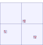
Figure 4: (a) A regular quadtree on a set of $\color[rgb]{0.75,0.30,0.15}8$ points. (b) A slight shift of the base square may cause many new compressed nodes in the quadtree.

In this section, we show that it is possible to “shift” a quadtree; that is, given a compressed quadtree on a set of points $\color[rgb]{0.75,0.30,0.15}P$ with base square $\color[rgb]{0.75,0.30,0.15}R$, to compute another compressed quadtree on $\color[rgb]{0.75,0.30,0.15}P$ with a base square that is similar to $\color[rgb]{0.75,0.30,0.15}R$, in linear time. The main difficulty lies in the fact that the clusters in the two quadtrees can be very different, as illustrated in Figure 4.

Theorem 3.7.

Suppose $\color[rgb]{0.75,0.30,0.15}a$ is a sufficiently large constant and $\color[rgb]{0.75,0.30,0.15}P$ a planar $\color[rgb]{0.75,0.30,0.15}n$-point set. Furthermore, let $\color[rgb]{0.75,0.30,0.15}T$ be an $\color[rgb]{0.75,0.30,0.15}a$-compressed quadtree for $\color[rgb]{0.75,0.30,0.15}P$ with base square $\color[rgb]{0.75,0.30,0.15}R$, and let $\color[rgb]{0.75,0.30,0.15}S$ be a square with $\color[rgb]{0.75,0.30,0.15}S\supseteq P$ and $\color[rgb]{0.75,0.30,0.15}|S|=\Theta(|R|)$. Then we can construct in $\color[rgb]{0.75,0.30,0.15}O(m)$ time a balanced $\color[rgb]{0.75,0.30,0.15}a$-compressed quadtree $\color[rgb]{0.75,0.30,0.15}T^{\prime}$ for $\color[rgb]{0.75,0.30,0.15}P$ with base square $\color[rgb]{0.75,0.30,0.15}S$ and with $\color[rgb]{0.75,0.30,0.15}O(m)$ nodes.

The idea is to construct $\color[rgb]{0.75,0.30,0.15}T^{\prime}$ in the traditional way through repeated subdivision of the base square $\color[rgb]{0.75,0.30,0.15}S$, while using the information provided by $\color[rgb]{0.75,0.30,0.15}T$ in order to speed up the point location. We will use the terms $\color[rgb]{0.75,0.30,0.15}T$-square and $\color[rgb]{0.75,0.30,0.15}T^{\prime}$-square to distinguish the squares in the two trees. During the subdivision process, we maintain the partial tree $\color[rgb]{0.75,0.30,0.15}T^{\prime}$, and for each square $\color[rgb]{0.75,0.30,0.15}S^{\prime}$ of $\color[rgb]{0.75,0.30,0.15}T^{\prime}$ we keep track of the $\color[rgb]{0.75,0.30,0.15}T$-squares that have similar size as $\color[rgb]{0.75,0.30,0.15}S^{\prime}$ and that intersect $\color[rgb]{0.75,0.30,0.15}S^{\prime}$ (in an associated set). We call the leaves of the current partial tree the frontier of $\color[rgb]{0.75,0.30,0.15}T^{\prime}$. In each step, we pick a frontier $\color[rgb]{0.75,0.30,0.15}T^{\prime}$-square and split it, until we have reached a valid quadtree for $\color[rgb]{0.75,0.30,0.15}P$. We need to be careful in order to keep $\color[rgb]{0.75,0.30,0.15}T^{\prime}$ balanced and in order to deal with compressed nodes. The former problem is handled by starting a cascading split operation as soon as a single split makes $\color[rgb]{0.75,0.30,0.15}T^{\prime}$ unbalanced. For the latter problem, we would like to treat the compressed children in the same way as the points in $\color[rgb]{0.75,0.30,0.15}P$, and handle them later recursively. However, there is a problem: during the balancing procedure, it may happen that a compressed child becomes too large for its parent square and should be part of the regular tree. In order to deal with this, we must keep track of the compressed children in the associated sets of the $\color[rgb]{0.75,0.30,0.15}T^{\prime}$-squares. When we detect that a compressed child has become too large for its parent, we treat it like a regular square. Once we are done, we recurse on the remaining compressed children. Through a charging scheme, we can show that the overall work is linear in the size of $\color[rgb]{0.75,0.30,0.15}T$. The following paragraphs describe the individual steps of the algorithm in more detail.

Initialization and Data Structures.

We obtain from $\color[rgb]{0.75,0.30,0.15}S$ a grid with squares of size in $\color[rgb]{0.75,0.30,0.15}(|R|/2,|R|]$, either by repeatedly subdividing $\color[rgb]{0.75,0.30,0.15}S$, if $\color[rgb]{0.75,0.30,0.15}|S|>|R|$; or by repeatedly doubling $\color[rgb]{0.75,0.30,0.15}S$, if $\color[rgb]{0.75,0.30,0.15}|S|\leq|R|/2$. Since $\color[rgb]{0.75,0.30,0.15}|S|=\Theta(|R|)$, this requires a constant number of steps. Then we determine the $\color[rgb]{0.75,0.30,0.15}T^{\prime}$-squares $\color[rgb]{0.75,0.30,0.15}S_{1}^{\prime},\dots,S_{k}^{\prime}$ of that grid that intersect $\color[rgb]{0.75,0.30,0.15}R$ (note that $\color[rgb]{0.75,0.30,0.15}k\leq 9$). Our algorithm maintains the following data structures: (i) a list $\color[rgb]{0.75,0.30,0.15}L$ of active $\color[rgb]{0.75,0.30,0.15}T^{\prime}$-squares; and (ii) for each $\color[rgb]{0.75,0.30,0.15}T^{\prime}$-square $\color[rgb]{0.75,0.30,0.15}S^{\prime}$ a list $\color[rgb]{0.75,0.30,0.15}\operatorname{as}(S^{\prime})$ of associated $\color[rgb]{0.75,0.30,0.15}T$-squares. We will maintain the invariant that $\color[rgb]{0.75,0.30,0.15}\operatorname{as}(S^{\prime})$ contains the smallest $\color[rgb]{0.75,0.30,0.15}T$-squares that have size at least $\color[rgb]{0.75,0.30,0.15}|S^{\prime}|$ and that intersect $\color[rgb]{0.75,0.30,0.15}S^{\prime}$, as well as any compressed children that are contained in such a $\color[rgb]{0.75,0.30,0.15}T$-square and that intersect $\color[rgb]{0.75,0.30,0.15}S^{\prime}$. This invariant implies that each $\color[rgb]{0.75,0.30,0.15}S^{\prime}$ has $\color[rgb]{0.75,0.30,0.15}O(1)$ associated squares. We call a $\color[rgb]{0.75,0.30,0.15}T^{\prime}$-square $\color[rgb]{0.75,0.30,0.15}S^{\prime}$ active if $\color[rgb]{0.75,0.30,0.15}\operatorname{as}(S^{\prime})$ contains a $\color[rgb]{0.75,0.30,0.15}T$-square of size in $\color[rgb]{0.75,0.30,0.15}[|S^{\prime}|,2|S^{\prime}|)$ or a compressed child of size in $\color[rgb]{0.75,0.30,0.15}[|S^{\prime}|/2^{2a},|S^{\prime}|)$. Initially, we set $\color[rgb]{0.75,0.30,0.15}L:=\{S_{1}^{\prime},\dots,S_{k}^{\prime}\}$ and $\color[rgb]{0.75,0.30,0.15}\operatorname{as}(S_{1}^{\prime})=\operatorname{as}(S_{2}^{\prime})=\dots=\operatorname{as}(S_{k}^{\prime})=\{R\}$, fulfilling the invariant.

The Split Operation.

The basic operation of our algorithm is the split. A split takes a $\color[rgb]{0.75,0.30,0.15}T^{\prime}$-square $\color[rgb]{0.75,0.30,0.15}S^{\prime}$ and subdivides it into four children $\color[rgb]{0.75,0.30,0.15}S^{\prime}_{1},\dots,S^{\prime}_{4}$. Then it computes the associated sets $\color[rgb]{0.75,0.30,0.15}\operatorname{as}(S^{\prime}_{1}),\dots,\operatorname{as}(S^{\prime}_{4})$ as follows. For each $\color[rgb]{0.75,0.30,0.15}i=1,\dots,4$, we intersect $\color[rgb]{0.75,0.30,0.15}S^{\prime}_{i}$ with all $\color[rgb]{0.75,0.30,0.15}T$-squares in $\color[rgb]{0.75,0.30,0.15}\operatorname{as}(S^{\prime})$, and we put those $\color[rgb]{0.75,0.30,0.15}T$-squares into $\color[rgb]{0.75,0.30,0.15}\operatorname{as}(S_{i}^{\prime})$ that have non-empty intersection with $\color[rgb]{0.75,0.30,0.15}S^{\prime}_{i}$. Then we replace each $\color[rgb]{0.75,0.30,0.15}T$-square in $\color[rgb]{0.75,0.30,0.15}\operatorname{as}(S^{\prime})$ that is neither a leaf, nor a compressed node, nor a compressed child by those of its children that have non-empty intersection with $\color[rgb]{0.75,0.30,0.15}S_{i}^{\prime}$. Finally, we remove from $\color[rgb]{0.75,0.30,0.15}\operatorname{as}(S_{i}^{\prime})$ those compressed nodes whose compressed children have size at least $\color[rgb]{0.75,0.30,0.15}|S_{i}^{\prime}|$ and intersect $\color[rgb]{0.75,0.30,0.15}S_{i}^{\prime}$. Having determined $\color[rgb]{0.75,0.30,0.15}\operatorname{as}(S^{\prime}_{i})$, we use it to check whether $\color[rgb]{0.75,0.30,0.15}S_{i}^{\prime}$ is active. If so, we add it to $\color[rgb]{0.75,0.30,0.15}L$. The split operation maintains the invariant about the associated sets, and it takes constant time.

Main Body and Point-Location.

We now describe the main body of our algorithm. It consists of phases. In each phase, we remove a $\color[rgb]{0.75,0.30,0.15}T^{\prime}$-square $\color[rgb]{0.75,0.30,0.15}S^{\prime}$ from $\color[rgb]{0.75,0.30,0.15}L$. We perform a split operation on $\color[rgb]{0.75,0.30,0.15}S^{\prime}$ as described above. Then, we start the balancing procedure. For this, we check the four $\color[rgb]{0.75,0.30,0.15}T^{\prime}$-squares in the current frontier that are directly above, below, to the left and to the right of $\color[rgb]{0.75,0.30,0.15}S^{\prime}$ to see whether any of them have size $\color[rgb]{0.75,0.30,0.15}2|S^{\prime}|$. We put each such $\color[rgb]{0.75,0.30,0.15}T^{\prime}$-square into a queue $\color[rgb]{0.75,0.30,0.15}Q$. Then, while $\color[rgb]{0.75,0.30,0.15}Q$ is not empty, we remove a square $\color[rgb]{0.75,0.30,0.15}N^{\prime}$ from $\color[rgb]{0.75,0.30,0.15}Q$ and perform a split operation on it (note that this may create new active squares). Furthermore, if $\color[rgb]{0.75,0.30,0.15}N^{\prime}$ is in $\color[rgb]{0.75,0.30,0.15}L$, we remove it from $\color[rgb]{0.75,0.30,0.15}L$. Finally, we consider the $\color[rgb]{0.75,0.30,0.15}T^{\prime}$-squares of the current frontier directly above, below, to the left and to the right of $\color[rgb]{0.75,0.30,0.15}N^{\prime}$. If any of them have size $\color[rgb]{0.75,0.30,0.15}2|N^{\prime}|$ and are not in $\color[rgb]{0.75,0.30,0.15}Q$ yet, we append them to $\color[rgb]{0.75,0.30,0.15}Q$ and continue. The balancing procedure, and hence the phase, ends once $\color[rgb]{0.75,0.30,0.15}Q$ is empty.

We continue this process until $\color[rgb]{0.75,0.30,0.15}L$ is empty. Next, we do point-location. Let $\color[rgb]{0.75,0.30,0.15}S^{\prime}$ be a $\color[rgb]{0.75,0.30,0.15}T^{\prime}$-square of the current frontier. Since $\color[rgb]{0.75,0.30,0.15}L$ is empty, $\color[rgb]{0.75,0.30,0.15}S^{\prime}$ is associated with $\color[rgb]{0.75,0.30,0.15}O(1)$ $\color[rgb]{0.75,0.30,0.15}T$-squares, all of which are either leaves or compressed nodes or compressed children in $\color[rgb]{0.75,0.30,0.15}T$. For each $\color[rgb]{0.75,0.30,0.15}T$-leaf that intersects $\color[rgb]{0.75,0.30,0.15}S^{\prime}$, we determine whether it contains a point that lies in $\color[rgb]{0.75,0.30,0.15}S^{\prime}$. In the end, we have a set of at most four points from $\color[rgb]{0.75,0.30,0.15}P$ or compressed children of $\color[rgb]{0.75,0.30,0.15}T$ that intersect $\color[rgb]{0.75,0.30,0.15}S^{\prime}$, and we call this set the secondary associated set for $\color[rgb]{0.75,0.30,0.15}S^{\prime}$, denoted by $\color[rgb]{0.75,0.30,0.15}\operatorname{as}_{2}(S^{\prime})$. We do this for every $\color[rgb]{0.75,0.30,0.15}T^{\prime}$-square in the current frontier.

The Secondary Stage.

Next, the goal is to build a small compressed quadtree for the secondary associated set of each square in the current frontier. Of course, the tree needs to remain balanced. For this, we start an operation that is similar to the main body of the algorithm. We call a $\color[rgb]{0.75,0.30,0.15}T^{\prime}$-square $\color[rgb]{0.75,0.30,0.15}S^{\prime}$ post-active if $\color[rgb]{0.75,0.30,0.15}|\operatorname{as}_{2}(S^{\prime})|\geq 2$ and the smallest bounding square for the elements in $\color[rgb]{0.75,0.30,0.15}\operatorname{as}_{2}(S^{\prime})$ has size larger than $\color[rgb]{0.75,0.30,0.15}|S^{\prime}|/128a$. We put all the post-active squares into a list $\color[rgb]{0.75,0.30,0.15}L_{2}$ and we proceed as before: we repeatedly take a post-active square from $\color[rgb]{0.75,0.30,0.15}L_{2}$, split it, and then perform a balancing procedure. Here, the splitting operation is as follows: given a square $\color[rgb]{0.75,0.30,0.15}S^{\prime}$, we split it into four children $\color[rgb]{0.75,0.30,0.15}S^{\prime}_{1},\ldots,S^{\prime}_{4}$. By comparing each child $\color[rgb]{0.75,0.30,0.15}S_{i}^{\prime}$ to each element in the secondary associated set $\color[rgb]{0.75,0.30,0.15}\operatorname{as}_{2}(S^{\prime})$, we determine the new secondary associated sets $\color[rgb]{0.75,0.30,0.15}\operatorname{as}_{2}(S^{\prime}_{1}),\ldots,\operatorname{as}_{2}(S^{\prime}_{4})$. We use these associated sets to check which children $\color[rgb]{0.75,0.30,0.15}S^{\prime}_{i}$ (if any) are post-active and add them to $\color[rgb]{0.75,0.30,0.15}L_{2}$, if necessary. This splitting operation takes constant time. Again, it may happen that the balancing procedure creates new post-active squares. We repeat this procedure until $\color[rgb]{0.75,0.30,0.15}L_{2}$ is empty.

Setting Up the Recursive Calls.

After the secondary stage, there are no more post-active squares, so for each square $\color[rgb]{0.75,0.30,0.15}S^{\prime}$ in the current frontier we have (i) $\color[rgb]{0.75,0.30,0.15}|\operatorname{as}_{2}(S^{\prime})|\leq 1$; or (ii) the smallest bounding square of $\color[rgb]{0.75,0.30,0.15}\operatorname{as}_{2}(S^{\prime})$ has size at most $\color[rgb]{0.75,0.30,0.15}|S^{\prime}|/128a$. Below in Lemma 3.9 we will argue that if $\color[rgb]{0.75,0.30,0.15}\operatorname{as}_{2}(S^{\prime})$ contains a single compressed child $\color[rgb]{0.75,0.30,0.15}C$, then $\color[rgb]{0.75,0.30,0.15}C$ has size at most $\color[rgb]{0.75,0.30,0.15}|S^{\prime}|/128a$. Thus, (ii) holds in any case. The goal now is to set up a recursive call of the algorithm to handle the remaining compressed children. Unfortunately, a compressed child may intersect several leaf $\color[rgb]{0.75,0.30,0.15}T^{\prime}$-squares, so we need to be careful about choosing the base squares for the recursion.

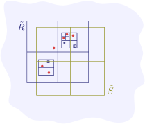
Figure 5: (a) A frontier square $\color[rgb]{0.75,0.30,0.15}S^{\prime}$ of $\color[rgb]{0.75,0.30,0.15}T^{\prime}$ intersects several compressed children of $\color[rgb]{0.75,0.30,0.15}T$. We identify the list $\color[rgb]{0.75,0.30,0.15}X$ of $\color[rgb]{0.75,0.30,0.15}T^{\prime}$ squares that intersect the same children. (b) To apply the shifting algorithm recursively, we choose base squares $\color[rgb]{0.75,0.30,0.15}\tilde{R}$ and $\color[rgb]{0.75,0.30,0.15}\tilde{S}$ aligned with $\color[rgb]{0.75,0.30,0.15}T$ and $\color[rgb]{0.75,0.30,0.15}T^{\prime}$.

Let $\color[rgb]{0.75,0.30,0.15}S^{\prime}$ be a square of the current frontier, and set $\color[rgb]{0.75,0.30,0.15}X:=\{S^{\prime}\}$. While there is a compressed child $\color[rgb]{0.75,0.30,0.15}C$ in $\color[rgb]{0.75,0.30,0.15}\operatorname{as}_{2}(X):=\bigcup_{S^{\prime\prime}\in X}\operatorname{as}_{2}(S^{\prime\prime})$ that intersects the boundary of $\color[rgb]{0.75,0.30,0.15}S(X):=\bigcup_{S^{\prime\prime}\in X}S^{\prime\prime}$, we add all the $\color[rgb]{0.75,0.30,0.15}T^{\prime}$-squares of the current frontier that are intersected by $\color[rgb]{0.75,0.30,0.15}C$ to $\color[rgb]{0.75,0.30,0.15}X$. Since $\color[rgb]{0.75,0.30,0.15}T^{\prime}$ is balanced, the $\color[rgb]{0.75,0.30,0.15}i$-th square $\color[rgb]{0.75,0.30,0.15}S^{(i)}$ that we add to $\color[rgb]{0.75,0.30,0.15}X$ has size at most $\color[rgb]{0.75,0.30,0.15}2^{i}|S^{\prime}|$ and hence the bounding square of $\color[rgb]{0.75,0.30,0.15}\operatorname{as}_{2}(S^{(i)})$ has size at most $\color[rgb]{0.75,0.30,0.15}2^{i}|S^{\prime}|/128a$. By construction, $\color[rgb]{0.75,0.30,0.15}\operatorname{as}_{2}(S^{(i)})$ contains at least one element that intersects a square in the old $\color[rgb]{0.75,0.30,0.15}X$, so by induction we know that after $\color[rgb]{0.75,0.30,0.15}i$ steps the set $\color[rgb]{0.75,0.30,0.15}\operatorname{as}_{2}(X)$ has a bounding square of size at most $\color[rgb]{0.75,0.30,0.15}2^{i+1}|S^{\prime}|/128a$. It follows that the process stops after at most three steps (i.e., when $\color[rgb]{0.75,0.30,0.15}X$ has four elements), because after four steps we would have a bounding square of size at most $\color[rgb]{0.75,0.30,0.15}2^{5}|S^{\prime}|/128a\leq|S^{\prime}|/4a$ that is intersected by five disjoint squares of size at least $\color[rgb]{0.75,0.30,0.15}|S^{\prime}|/2^{4}=|S^{\prime}|/16$ (since $\color[rgb]{0.75,0.30,0.15}T^{\prime}$ is balanced), which is impossible (for $\color[rgb]{0.75,0.30,0.15}a$ large enough). Figure 5 shows an example.

Now we put two base squares around $\color[rgb]{0.75,0.30,0.15}\operatorname{as}_{2}(X)$: a square $\color[rgb]{0.75,0.30,0.15}\widetilde{R}$ that is aligned with $\color[rgb]{0.75,0.30,0.15}T$, and a square $\color[rgb]{0.75,0.30,0.15}\widetilde{S}$ that is aligned with $\color[rgb]{0.75,0.30,0.15}T^{\prime}$. For $\color[rgb]{0.75,0.30,0.15}\widetilde{R}$, if $\color[rgb]{0.75,0.30,0.15}\operatorname{as}_{2}(X)$ contains only one element, we just use the bounding square of $\color[rgb]{0.75,0.30,0.15}\operatorname{as}_{2}(X)$. If $\color[rgb]{0.75,0.30,0.15}|\operatorname{as}_{2}(X)|\geq 2$, then the elements of $\color[rgb]{0.75,0.30,0.15}\operatorname{as}_{2}(X)$ are separated by an edge or a corner between leaf $\color[rgb]{0.75,0.30,0.15}T$-squares. Thus, we can pick a base square $\color[rgb]{0.75,0.30,0.15}\widetilde{R}$ for $\color[rgb]{0.75,0.30,0.15}\operatorname{as}_{2}(X)$ such that (i) $\color[rgb]{0.75,0.30,0.15}|\widetilde{R}|\leq 2^{6}|S^{\prime}|/128a=|S^{\prime}|/2a$; (ii) $\color[rgb]{0.75,0.30,0.15}\widetilde{R}$ is aligned with $\color[rgb]{0.75,0.30,0.15}T$; and (iii) the first split of $\color[rgb]{0.75,0.30,0.15}\widetilde{R}$ separates the elements in $\color[rgb]{0.75,0.30,0.15}\operatorname{as}_{2}(X)$. For $\color[rgb]{0.75,0.30,0.15}\widetilde{S}$, if $\color[rgb]{0.75,0.30,0.15}|X|=1$, we just use the bounding square for $\color[rgb]{0.75,0.30,0.15}\operatorname{as}_{2}(X)$. If $\color[rgb]{0.75,0.30,0.15}|X|\geq 2$, the squares in $\color[rgb]{0.75,0.30,0.15}X$ must share a common edge or corner, and we can find a base square $\color[rgb]{0.75,0.30,0.15}\widetilde{S}$ such that (i) $\color[rgb]{0.75,0.30,0.15}\widetilde{S}$ contains $\color[rgb]{0.75,0.30,0.15}\operatorname{as}_{2}(X)$; (ii) the first split of $\color[rgb]{0.75,0.30,0.15}\widetilde{S}$ produces squares that are aligned with this edge or corner of $\color[rgb]{0.75,0.30,0.15}X$; and (iii) $\color[rgb]{0.75,0.30,0.15}|\widetilde{S}|\leq 2^{6}|S^{\prime}|/128a=|S^{\prime}|/2a$. Figure 5 shows an example. We now construct an $\color[rgb]{0.75,0.30,0.15}a$-compressed quadtree $\color[rgb]{0.75,0.30,0.15}\widetilde{T}$ with base square $\color[rgb]{0.75,0.30,0.15}\widetilde{R}$ for the elements of $\color[rgb]{0.75,0.30,0.15}\operatorname{as}_{2}(X)$ in the obvious way. (If $\color[rgb]{0.75,0.30,0.15}\operatorname{as}_{2}(X)$ contains any compressed children, we reuse them as compressed children for $\color[rgb]{0.75,0.30,0.15}\widetilde{T}$. This may lead to a violation of the condition for compressed nodes at the first level of $\color[rgb]{0.75,0.30,0.15}\widetilde{T}$. However, our algorithm automatically treats large compressed children as active squares, so there is no problem.) This takes constant time. We call the algorithm recursively to shift $\color[rgb]{0.75,0.30,0.15}\widetilde{T}$ to the new base square $\color[rgb]{0.75,0.30,0.15}\widetilde{S}$. Note that this leads to a valid $\color[rgb]{0.75,0.30,0.15}a$-compressed quadtree since either $\color[rgb]{0.75,0.30,0.15}\widetilde{S}$ is wholly contained in $\color[rgb]{0.75,0.30,0.15}S^{\prime}$; or the first split of $\color[rgb]{0.75,0.30,0.15}\widetilde{S}$ produces squares that are wholly contained in the $\color[rgb]{0.75,0.30,0.15}T^{\prime}$-leaf squares and have size at most $\color[rgb]{0.75,0.30,0.15}|S^{\prime}|/4a$, while each square that intersects $\color[rgb]{0.75,0.30,0.15}\widetilde{S}$ has size at least $\color[rgb]{0.75,0.30,0.15}|S^{\prime}|/4$, as $\color[rgb]{0.75,0.30,0.15}T^{\prime}$ is balanced. We repeat the procedure for every leaf $\color[rgb]{0.75,0.30,0.15}T^{\prime}$-square whose secondary associated set we have not processed yet.

Analysis.

The resulting tree $\color[rgb]{0.75,0.30,0.15}T^{\prime}$ is a balanced $\color[rgb]{0.75,0.30,0.15}a$-compressed quadtree for $\color[rgb]{0.75,0.30,0.15}P$. It remains to prove that the algorithm runs in linear time. The initialization stage needs $\color[rgb]{0.75,0.30,0.15}O(1)$ steps. Next, we consider the main body of the algorithm. Since each split takes constant time, the total running time for the main body is proportional to the number of splits. Recall that a $\color[rgb]{0.75,0.30,0.15}T^{\prime}$-square $\color[rgb]{0.75,0.30,0.15}S^{\prime}$ is called active if it is put into $\color[rgb]{0.75,0.30,0.15}L$, i.e., if $\color[rgb]{0.75,0.30,0.15}\operatorname{as}(S^{\prime})$ contains a $\color[rgb]{0.75,0.30,0.15}T$-square of size in $\color[rgb]{0.75,0.30,0.15}[|S^{\prime}|,2|S^{\prime}|)$ or a compressed child of size in $\color[rgb]{0.75,0.30,0.15}(|S^{\prime}|/2^{2a},|S^{\prime}|]$. Since each $\color[rgb]{0.75,0.30,0.15}T$-square can cause only a constant number of $\color[rgb]{0.75,0.30,0.15}T^{\prime}$-squares to be active, the total number of active $\color[rgb]{0.75,0.30,0.15}T^{\prime}$-squares is $\color[rgb]{0.75,0.30,0.15}O(m)$. Thus, we can use the following lemma to conclude that the total number of splits in the main body of the algorithm is linear.

Lemma 3.8.

Every split in the main body of the algorithm can be charged to an active $\color[rgb]{0.75,0.30,0.15}T^{\prime}$-square such that each such square is charged a constant number of times.

Proof.

If we split an active square $\color[rgb]{0.75,0.30,0.15}S^{\prime}$, we can trivially charge the split to $\color[rgb]{0.75,0.30,0.15}S^{\prime}$. Hence, the critical splits are the ones during the balancing procedure. By induction on the number of steps of the balancing procedure, we see that if a square $\color[rgb]{0.75,0.30,0.15}S^{\prime}$ is split, there must be a square $\color[rgb]{0.75,0.30,0.15}N^{\prime}$ in the current partial tree $\color[rgb]{0.75,0.30,0.15}T^{\prime}$ that is a direct neighbor of $\color[rgb]{0.75,0.30,0.15}S^{\prime}$ and that has an active descendant whose removal from $\color[rgb]{0.75,0.30,0.15}L$ triggered the balancing procedure.

If $\color[rgb]{0.75,0.30,0.15}N^{\prime}$ has an active ancestor $\color[rgb]{0.75,0.30,0.15}\widetilde{N}$ that is at most five levels above $\color[rgb]{0.75,0.30,0.15}N^{\prime}$ in $\color[rgb]{0.75,0.30,0.15}T^{\prime}$ (possibly $\color[rgb]{0.75,0.30,0.15}\widetilde{N}=N^{\prime}$), we charge the split of $\color[rgb]{0.75,0.30,0.15}S^{\prime}$ to $\color[rgb]{0.75,0.30,0.15}\widetilde{N}$, and we are done. Otherwise, we know that $\color[rgb]{0.75,0.30,0.15}\operatorname{as}(N^{\prime})$ contains at least one compressed child of size less than $\color[rgb]{0.75,0.30,0.15}|N^{\prime}|/2^{2a}$ (otherwise, $\color[rgb]{0.75,0.30,0.15}N^{\prime}$ would not have an active descendant or would itself be active) and $\color[rgb]{0.75,0.30,0.15}T$-squares of size at least $\color[rgb]{0.75,0.30,0.15}64|N^{\prime}|$ (otherwise, one of the five nodes above $\color[rgb]{0.75,0.30,0.15}N^{\prime}$ in $\color[rgb]{0.75,0.30,0.15}T^{\prime}$ would have been active). Now, before $\color[rgb]{0.75,0.30,0.15}S^{\prime}$ is split, there must have been a split on $\color[rgb]{0.75,0.30,0.15}N^{\prime}$: otherwise the active descendant of $\color[rgb]{0.75,0.30,0.15}N^{\prime}$ that triggers the split on $\color[rgb]{0.75,0.30,0.15}S^{\prime}$ would not exist. Thus, we repeat the argument to show that $\color[rgb]{0.75,0.30,0.15}N^{\prime}$ has a direct neighbor $\color[rgb]{0.75,0.30,0.15}N^{\prime\prime}$ with an active descendant that triggers the split of $\color[rgb]{0.75,0.30,0.15}S^{\prime}$. Note that $\color[rgb]{0.75,0.30,0.15}N^{\prime\prime}\neq S^{\prime}$, because the split on $\color[rgb]{0.75,0.30,0.15}N^{\prime}$ happens before the split on $\color[rgb]{0.75,0.30,0.15}S^{\prime}$. If $\color[rgb]{0.75,0.30,0.15}N^{\prime\prime}$ has an active ancestor that is at most five levels higher up in $\color[rgb]{0.75,0.30,0.15}T^{\prime}$ (possibly $\color[rgb]{0.75,0.30,0.15}N^{\prime\prime}$ itself), we are done again. Otherwise, we repeat the argument again.

We claim that this process finishes after at most $\color[rgb]{0.75,0.30,0.15}16$ steps. Indeed, suppose we find $\color[rgb]{0.75,0.30,0.15}17$ squares $\color[rgb]{0.75,0.30,0.15}S^{\prime}=N^{(0)},N^{(1)},N^{(2)},\ldots,N^{(17)}$ without stopping. We know that each $\color[rgb]{0.75,0.30,0.15}N^{(j)}$ is a direct neighbor of $\color[rgb]{0.75,0.30,0.15}N^{(j-1)}$ and that each $\color[rgb]{0.75,0.30,0.15}N^{(j)}$ is associated with a compressed child of size at most $\color[rgb]{0.75,0.30,0.15}|S^{\prime}|/2^{2a}$ and with $\color[rgb]{0.75,0.30,0.15}T$-squares of size at least $\color[rgb]{0.75,0.30,0.15}64|S^{\prime}|$. Since the set $\color[rgb]{0.75,0.30,0.15}\bigcup_{j=0}^{16}N^{(j)}$ has diameter at most $\color[rgb]{0.75,0.30,0.15}17|S^{\prime}|$, the set $\color[rgb]{0.75,0.30,0.15}\bigcup_{j=0}^{16}\operatorname{as}(N^{(j)})$ contains at most four $\color[rgb]{0.75,0.30,0.15}T$-squares of size at least $\color[rgb]{0.75,0.30,0.15}64|S^{\prime}|$. Now each compressed child in an associated set $\color[rgb]{0.75,0.30,0.15}\operatorname{as}(N^{(j)})$ is the only child of one of these four large $\color[rgb]{0.75,0.30,0.15}T$-squares, so there are at most four of them. Furthermore, each such compressed child is intersected by at most four disjoint $\color[rgb]{0.75,0.30,0.15}T$-squares of size $\color[rgb]{0.75,0.30,0.15}|S^{\prime}|$, so there can be at most $\color[rgb]{0.75,0.30,0.15}16$ squares $\color[rgb]{0.75,0.30,0.15}N^{(j)}$, a contradiction. Hence, we can charge each split to an active square in the desired fashion, and the lemma follows. ∎

Next, we analyze the running time of the secondary stage. Again, the running time is proportional to the number of splits, which is bounded by the following lemma.

Lemma 3.9.

Let $\color[rgb]{0.75,0.30,0.15}S^{\prime}$ be a frontier $\color[rgb]{0.75,0.30,0.15}T^{\prime}$-square at the beginning of the secondary stage. Then after the secondary stage, the subtree rooted at $\color[rgb]{0.75,0.30,0.15}S^{\prime}$ has height at most $\color[rgb]{0.75,0.30,0.15}O(\log a)$.

Proof.

Below, we will argue that for every descendant $\color[rgb]{0.75,0.30,0.15}S^{\prime\prime}$ of $\color[rgb]{0.75,0.30,0.15}S^{\prime}$, if $\color[rgb]{0.75,0.30,0.15}\operatorname{as}_{2}(S^{\prime\prime})$ contains a compressed child $\color[rgb]{0.75,0.30,0.15}C$, then $\color[rgb]{0.75,0.30,0.15}|C|\leq|S^{\prime\prime}|/2^{a}$. For now, suppose that this holds.

First, we claim that there are $\color[rgb]{0.75,0.30,0.15}O(\log a)$ splits to post-active descendants of $\color[rgb]{0.75,0.30,0.15}S^{\prime}$. The secondary associated set $\color[rgb]{0.75,0.30,0.15}\operatorname{as}_{2}(S^{\prime})$ contains at most four elements, so $\color[rgb]{0.75,0.30,0.15}\operatorname{as}_{2}(S^{\prime})$ has at most $\color[rgb]{0.75,0.30,0.15}11$ subsets with two or more elements. Fix such a subset $\color[rgb]{0.75,0.30,0.15}\mathcal{A}$. Then $\color[rgb]{0.75,0.30,0.15}S^{\prime}$ has at most $\color[rgb]{0.75,0.30,0.15}O(\log a)$ post-active descendants with secondary associated set $\color[rgb]{0.75,0.30,0.15}\mathcal{A}$. This is because each level of $\color[rgb]{0.75,0.30,0.15}T^{\prime}$ has at most two squares with secondary associated set $\color[rgb]{0.75,0.30,0.15}\mathcal{A}$, and the post-active squares with secondary associated set $\color[rgb]{0.75,0.30,0.15}\mathcal{A}$ must have size between $\color[rgb]{0.75,0.30,0.15}|B(\mathcal{A})|/2$ and $\color[rgb]{0.75,0.30,0.15}128a|B(\mathcal{A})|$, where $\color[rgb]{0.75,0.30,0.15}B(\mathcal{A})$ denotes the smallest bounding square for the elements in $\color[rgb]{0.75,0.30,0.15}\mathcal{A}$. (Here we use our claim that the compressed children in the secondary associated set of each frontier $\color[rgb]{0.75,0.30,0.15}T^{\prime}$-square $\color[rgb]{0.75,0.30,0.15}S^{\prime\prime}$ are much smaller than $\color[rgb]{0.75,0.30,0.15}S^{\prime\prime}$.) There are only $\color[rgb]{0.75,0.30,0.15}O(\log a)$ such levels, so adding over all $\color[rgb]{0.75,0.30,0.15}\mathcal{A}$, we see that $\color[rgb]{0.75,0.30,0.15}S^{\prime}$ has at most $\color[rgb]{0.75,0.30,0.15}O(\log a)$ post-active descendants, implying the claim.

Each split creates at most one new level below $\color[rgb]{0.75,0.30,0.15}S^{\prime}$, so there are only $\color[rgb]{0.75,0.30,0.15}O(\log a)$ new levels due to splits to post-active descendants of $\color[rgb]{0.75,0.30,0.15}S^{\prime}$. Next, we bound the number of new levels that are created by splits during the balancing phases. Each balancing phase creates at most one new level below $\color[rgb]{0.75,0.30,0.15}S^{\prime}$. Furthermore, by induction on the number of steps in the balancing phase, we see that the balancing phase was triggered by the split of a post-active square that is a descendant either of $\color[rgb]{0.75,0.30,0.15}S^{\prime}$ or of a direct neighbor of $\color[rgb]{0.75,0.30,0.15}S^{\prime}$. At the beginning of the secondary stage, there are $\color[rgb]{0.75,0.30,0.15}O(1)$ $\color[rgb]{0.75,0.30,0.15}T^{\prime}$-squares that are descendants of direct neighbors of $\color[rgb]{0.75,0.30,0.15}S^{\prime}$ (as $\color[rgb]{0.75,0.30,0.15}T^{\prime}$ is balanced). As we argued above, each of them has at most $\color[rgb]{0.75,0.30,0.15}O(\log a)$ post-active descendants. Thus, the balancing phases add at most $\color[rgb]{0.75,0.30,0.15}O(\log a)$ new levels below $\color[rgb]{0.75,0.30,0.15}S^{\prime}$.

Finally, we need to justify the assumption that for any descendant $\color[rgb]{0.75,0.30,0.15}S^{\prime\prime}$ with a compressed child $\color[rgb]{0.75,0.30,0.15}C\in\operatorname{as}_{2}(S^{\prime\prime})$, we have $\color[rgb]{0.75,0.30,0.15}|C|\leq|S^{\prime\prime}|/2^{a}$. By construction, we have $\color[rgb]{0.75,0.30,0.15}|C|\leq|S^{\prime}|/2^{2a}$. Suppose that $\color[rgb]{0.75,0.30,0.15}S^{\prime}$ has a descendant $\color[rgb]{0.75,0.30,0.15}S^{\prime\prime}$ that violates this assumption. The square $\color[rgb]{0.75,0.30,0.15}S^{\prime\prime}$ was created through a split in the secondary stage, and suppose that $\color[rgb]{0.75,0.30,0.15}S^{\prime\prime}$ is the first such square during the whole secondary stage. This means that during all previous splits, the assumption holds, so by the argument above, there are at most $\color[rgb]{0.75,0.30,0.15}O(\log a)$ levels below $\color[rgb]{0.75,0.30,0.15}S^{\prime}$. This means that $\color[rgb]{0.75,0.30,0.15}|S^{\prime\prime}|\geq|S^{\prime}|/a^{O(1)}$, so we would get $\color[rgb]{0.75,0.30,0.15}|S^{\prime}|/2^{2a}\geq|C|>|S^{\prime\prime}|/2^{a}>|S^{\prime}|/2^{2a}$, a contradiction (for $\color[rgb]{0.75,0.30,0.15}a$ large enough). Thus, no $\color[rgb]{0.75,0.30,0.15}S^{\prime\prime}$ can violate the assumption, as desired. ∎

The time to set up the recursion is constant for each square of the current frontier. From Lemmas 3.8 and 3.9, we can conclude that the total time of the algorithm is $\color[rgb]{0.75,0.30,0.15}O(m)$, which also implies that $\color[rgb]{0.75,0.30,0.15}T^{\prime}$ has $\color[rgb]{0.75,0.30,0.15}O(m)$ squares. This concludes the proof of Theorem 3.7.

Special Cases.

We note two useful special cases of Theorem 3.7. The first one gives an analog of Theorem 3.2 for compressed quadtrees.

Corollary 3.10.

Let $\color[rgb]{0.75,0.30,0.15}T$ be a $\color[rgb]{0.75,0.30,0.15}a$-compressed quadtree with $\color[rgb]{0.75,0.30,0.15}m$ nodes. There exists a balanced $\color[rgb]{0.75,0.30,0.15}a$-compressed quadtree that contains $\color[rgb]{0.75,0.30,0.15}T$, has $\color[rgb]{0.75,0.30,0.15}O(m)$ nodes and can be constructed in $\color[rgb]{0.75,0.30,0.15}O(m)$ time.

Proof.

Let $\color[rgb]{0.75,0.30,0.15}R$ be the base square of $\color[rgb]{0.75,0.30,0.15}T$. We apply Theorem 3.7 with $\color[rgb]{0.75,0.30,0.15}S=R$. ∎

The second special case says that we can realign an uncompressed quadtree locally in any way we want, as long as we are willing to relax the definition of quadtree slightly. Let $\color[rgb]{0.75,0.30,0.15}P$ be a planar point set. We call a quadtree for $\color[rgb]{0.75,0.30,0.15}P$ $\color[rgb]{0.75,0.30,0.15}\lambda$-relaxed if it has at most $\color[rgb]{0.75,0.30,0.15}\lambda$ points of $\color[rgb]{0.75,0.30,0.15}P$ in each leaf, and is otherwise a regular quadtree.

Corollary 3.11.

Let $\color[rgb]{0.75,0.30,0.15}P$ be a planar point set and $\color[rgb]{0.75,0.30,0.15}T$ a regular quadtree for $\color[rgb]{0.75,0.30,0.15}P$, with base square $\color[rgb]{0.75,0.30,0.15}R$. Let $\color[rgb]{0.75,0.30,0.15}S$ be another square with $\color[rgb]{0.75,0.30,0.15}S\supseteq P$ and $\color[rgb]{0.75,0.30,0.15}|S|=\Theta(|R|)$. Then we can build a $\color[rgb]{0.75,0.30,0.15}4$-relaxed quadtree $\color[rgb]{0.75,0.30,0.15}T^{\prime}$ for $\color[rgb]{0.75,0.30,0.15}P$ with base square $\color[rgb]{0.75,0.30,0.15}S$ in $\color[rgb]{0.75,0.30,0.15}O(|T|)$ time such that $\color[rgb]{0.75,0.30,0.15}T^{\prime}$ has $\color[rgb]{0.75,0.30,0.15}O(|T|)$ nodes.

Proof.

We apply Theorem 3.7 to $\color[rgb]{0.75,0.30,0.15}T$, but we stop the algorithm before the beginning of the secondary stage. Since each secondary associated set for a leaf square has at most four elements, and since $\color[rgb]{0.75,0.30,0.15}T$ contains no compressed nodes, the resulting tree $\color[rgb]{0.75,0.30,0.15}T^{\prime}$ has the desired properties. ∎

3.3 Equivalence of Compressed and $\color[rgb]{0.75,0.30,0.15}c$-Cluster Quadtrees

The goal of this section is to prove the following theorem.

Theorem 3.12.

Let $\color[rgb]{0.75,0.30,0.15}P$ be a planar $\color[rgb]{0.75,0.30,0.15}n$-point set. Given a $\color[rgb]{0.75,0.30,0.15}(c_{1},c_{2})$-cluster quadtree on $\color[rgb]{0.75,0.30,0.15}P$, we can compute in $\color[rgb]{0.75,0.30,0.15}O(n)$ time an $\color[rgb]{0.75,0.30,0.15}O(c_{1})$-compressed quadtree on $\color[rgb]{0.75,0.30,0.15}P$; and given an $\color[rgb]{0.75,0.30,0.15}a$-compressed quadtree on $\color[rgb]{0.75,0.30,0.15}P$, we can compute in $\color[rgb]{0.75,0.30,0.15}O(n)$ time an $\color[rgb]{0.75,0.30,0.15}(a^{1/5},2a^{1/5})$-cluster quadtree on $\color[rgb]{0.75,0.30,0.15}P$.

We present the proof of Theorem 3.12 in two lemmas.

Lemma 3.13.

Let $\color[rgb]{0.75,0.30,0.15}P$ be a planar $\color[rgb]{0.75,0.30,0.15}n$-point set. Given a $\color[rgb]{0.75,0.30,0.15}(c_{1},c_{2})$-cluster quadtree $\color[rgb]{0.75,0.30,0.15}T$ for $\color[rgb]{0.75,0.30,0.15}P$, we can compute in linear time an $\color[rgb]{0.75,0.30,0.15}O(c_{1})$-compressed quadtree $\color[rgb]{0.75,0.30,0.15}T^{\prime}$ on $\color[rgb]{0.75,0.30,0.15}P$.

Proof.

We construct the compressed quadtree in a top-down fashion, beginning from the root. Suppose that we have constructed a partial compressed quadtree $\color[rgb]{0.75,0.30,0.15}T^{\prime}$, and let $\color[rgb]{0.75,0.30,0.15}q$ be the representative point for a node $\color[rgb]{0.75,0.30,0.15}u$ in the $\color[rgb]{0.75,0.30,0.15}(c_{1},c_{2})$-cluster tree $\color[rgb]{0.75,0.30,0.15}T_{(c_{1},c_{2})}$ that corresponds to $\color[rgb]{0.75,0.30,0.15}T$. We show how to expand $\color[rgb]{0.75,0.30,0.15}q$ in $\color[rgb]{0.75,0.30,0.15}T^{\prime}$ to the corresponding quadtree $\color[rgb]{0.75,0.30,0.15}T_{u}^{Q}$.

First, we add to $\color[rgb]{0.75,0.30,0.15}T_{u}^{Q}$ a new root that is aligned with the old base square and larger by a constant factor, such that the old base square does not touch any boundary of the new one. Next, we determine by a search from $\color[rgb]{0.75,0.30,0.15}q$ which leaf squares of $\color[rgb]{0.75,0.30,0.15}T^{\prime}$ intersect $\color[rgb]{0.75,0.30,0.15}T_{u}^{Q}$. By Observation 3.3, there are at most four such leaves, so this step takes constant time. (Note that since we grow the base square of each quadtree that we expand, it cannot happen that $\color[rgb]{0.75,0.30,0.15}T_{u}^{Q}$ intersects the boundary of its parent quadtree.) Next, we repeatedly split each leaf that intersects $\color[rgb]{0.75,0.30,0.15}T_{u}^{Q}$ and that contains some other point or compressed child until there are no more such leaves.

The proof of Observation 3.3 shows that every leaf square of $\color[rgb]{0.75,0.30,0.15}T^{\prime}$ that intersects $\color[rgb]{0.75,0.30,0.15}T_{u}^{Q}$ has size at least $\color[rgb]{0.75,0.30,0.15}c_{1}d/4$, where $\color[rgb]{0.75,0.30,0.15}d$ is the size of $\color[rgb]{0.75,0.30,0.15}T_{u}^{Q}$’s base square. If $\color[rgb]{0.75,0.30,0.15}T_{u}^{Q}$ lies completely inside a leaf of $\color[rgb]{0.75,0.30,0.15}T^{\prime}$, we add $\color[rgb]{0.75,0.30,0.15}T_{u}^{Q}$ as a compressed child to $\color[rgb]{0.75,0.30,0.15}T^{\prime}$. If $\color[rgb]{0.75,0.30,0.15}T_{u}^{Q}$ intersects more than one leaf square, we identify a square at most twice the size of $\color[rgb]{0.75,0.30,0.15}T_{u}^{Q}$’s base square that is aligned appropriately with the relevant edges of $\color[rgb]{0.75,0.30,0.15}T$, and apply Corollary 3.11 to shift $\color[rgb]{0.75,0.30,0.15}T_{u}^{Q}$ to this new base square. This results in a valid $\color[rgb]{0.75,0.30,0.15}O(c_{1})$ compressed quadtree in which $\color[rgb]{0.75,0.30,0.15}q$ has been expanded. We repeat this process until all the quadtree pieces of $\color[rgb]{0.75,0.30,0.15}T$ have been integrated into a large compressed quadtree.

The total time for the top-down traversal and for the realignment procedures is linear. Furthermore, Corollary 3.6 shows that the total work for splitting the leaves of $\color[rgb]{0.75,0.30,0.15}T^{\prime}$ is also linear, since the points in the different clusters are $\color[rgb]{0.75,0.30,0.15}(1/c_{1})$-semi-separated. Hence, the total running time is linear. ∎

Lemma 3.14.

Let $\color[rgb]{0.75,0.30,0.15}P$ be a planar $\color[rgb]{0.75,0.30,0.15}n$-point set, and $\color[rgb]{0.75,0.30,0.15}T$ be an $\color[rgb]{0.75,0.30,0.15}a$-compressed quadtree for $\color[rgb]{0.75,0.30,0.15}P$. Then we can compute in linear time a $\color[rgb]{0.75,0.30,0.15}(a^{1/5},2a^{1/5})$-cluster quadtree for $\color[rgb]{0.75,0.30,0.15}P$.

Proof.

We use Corollary 3.10 to balance $\color[rgb]{0.75,0.30,0.15}T$, but without the recursive calls for the remaining cluster nodes. This gives a balanced top-level quadtree $\color[rgb]{0.75,0.30,0.15}T_{\text{top}}$ (possibly with some compressed children of $\color[rgb]{0.75,0.30,0.15}T$ now integrated in the tree), in which each leaf square is associated with at most four points from $\color[rgb]{0.75,0.30,0.15}P$ or compressed children of $\color[rgb]{0.75,0.30,0.15}T$. Furthermore, for each leaf square $\color[rgb]{0.75,0.30,0.15}S$ of $\color[rgb]{0.75,0.30,0.15}T_{\text{top}}$, we have a bounding square for the associated elements that is aligned with $\color[rgb]{0.75,0.30,0.15}T$ and has size at most $\color[rgb]{0.75,0.30,0.15}|S|/a$.

We use $\color[rgb]{0.75,0.30,0.15}T_{\text{top}}$ to identify a partial cluster quadtree, and we then recurse on the compressed children. We say a square $\color[rgb]{0.75,0.30,0.15}S\in T_{\text{top}}$ is full if there is a leaf below $\color[rgb]{0.75,0.30,0.15}S$ with a non-empty associated set. Otherwise, $\color[rgb]{0.75,0.30,0.15}S$ is empty. First, we consider the squares of $\color[rgb]{0.75,0.30,0.15}T_{\text{top}}$ in top-down fashion and check for each full square $\color[rgb]{0.75,0.30,0.15}S$ which direct neighbors of $\color[rgb]{0.75,0.30,0.15}S$ are empty (this can be done in constant time since $\color[rgb]{0.75,0.30,0.15}T$ is balanced). If $\color[rgb]{0.75,0.30,0.15}S$ has at most three full direct neighbors, and if all these full squares share a common corner, we let $\color[rgb]{0.75,0.30,0.15}U$ be a square that is aligned with $\color[rgb]{0.75,0.30,0.15}S$ and contains the full squares (i.e., either $\color[rgb]{0.75,0.30,0.15}U=S$ or $\color[rgb]{0.75,0.30,0.15}U$ is a square of size $\color[rgb]{0.75,0.30,0.15}2|S|$ that contains $\color[rgb]{0.75,0.30,0.15}S$ and its full neighbors). Next, we consider the squares of size $\color[rgb]{0.75,0.30,0.15}|U|$ in the $\color[rgb]{0.75,0.30,0.15}(4a^{1/5}+1)\times(4a^{1/5}+1)$ grid centered at $\color[rgb]{0.75,0.30,0.15}U$ and check whether they are all empty (again, since $\color[rgb]{0.75,0.30,0.15}T$ is balanced, this takes constant time). If so, the points associated with $\color[rgb]{0.75,0.30,0.15}U$ define a $\color[rgb]{0.75,0.30,0.15}a^{1/5}$-cluster. We put a representative point for the cluster into $\color[rgb]{0.75,0.30,0.15}U$, make a new quadtree with root $\color[rgb]{0.75,0.30,0.15}U$, and remove $\color[rgb]{0.75,0.30,0.15}U$’s children from $\color[rgb]{0.75,0.30,0.15}T_{\text{top}}$. We continue until all the squares of $\color[rgb]{0.75,0.30,0.15}T_{\text{top}}$ have been traversed, and then we process all the new trees in a similar way, iterating if necessary. After we are done, a part of the cluster quadtree has been created, and we need to consider the compressed children to set up a recursion.

For this, we consider each non-empty leaf square $\color[rgb]{0.75,0.30,0.15}S$ of the partial tree. Let $\color[rgb]{0.75,0.30,0.15}B$ be the bounding square of the associated elements of $\color[rgb]{0.75,0.30,0.15}S$. We know that $\color[rgb]{0.75,0.30,0.15}|B|\leq|S|/a$, so the disc $\color[rgb]{0.75,0.30,0.15}D$ of radius $\color[rgb]{0.75,0.30,0.15}2|B|a^{1/5}$ centered at $\color[rgb]{0.75,0.30,0.15}B$ intersects at most three other leaf squares. We check for each of these leaf squares whether $\color[rgb]{0.75,0.30,0.15}D$ intersects the bounding square of its associated elements. If so, we make a new bounding square for the union of these elements and repeat. This can happen at most twice more, because in each step the size of the bounding square increases by a factor of at most $\color[rgb]{0.75,0.30,0.15}a^{1/5}$. Hence, after three steps we have a disk $\color[rgb]{0.75,0.30,0.15}D$ of radius $\color[rgb]{0.75,0.30,0.15}O(|B|a^{4/5})$ that intersects four disjoint squares of size $\color[rgb]{0.75,0.30,0.15}\Omega(|B|a)$ that share a corner. Thus, $\color[rgb]{0.75,0.30,0.15}D$ must be completely contained in those squares. This also implies that this procedure yields a $\color[rgb]{0.75,0.30,0.15}a^{1/5}$-cluster. For each such cluster, we create a representative point and an appropriate base square for the child quadtree. Then, we process the cluster recursively. In the end, we can prune the resulting compressed trees to remove unnecessary nodes.

By the proof of Corollary 3.10, and since be spend only constant additional time for each square, this procedure takes linear time. Furthermore, as we argued above, we create only $\color[rgb]{0.75,0.30,0.15}a^{1/5}$-clusters. If $\color[rgb]{0.75,0.30,0.15}Q\subset P$ is a $\color[rgb]{0.75,0.30,0.15}2a^{1/5}$-cluster, then $\color[rgb]{0.75,0.30,0.15}Q$ is either contained in at most four leaf squares of $\color[rgb]{0.75,0.30,0.15}T_{\text{top}}$ that share a corner or the bounding square $\color[rgb]{0.75,0.30,0.15}B_{Q}$ intersects at most four squares of $\color[rgb]{0.75,0.30,0.15}T_{\text{top}}$ of size $\color[rgb]{0.75,0.30,0.15}\Theta(|B_{Q}|)$ such that the surrounding $\color[rgb]{0.75,0.30,0.15}(4a^{1/5}+1)\times(4a^{1/5}+1)$ grid contains only empty squares. In either case, $\color[rgb]{0.75,0.30,0.15}Q$ (or a superset) is discovered. It follows that the result is a valid $\color[rgb]{0.75,0.30,0.15}(a^{1/5},2a^{1/5})$-cluster quadtree. ∎

4 From a $\color[rgb]{0.75,0.30,0.15}c$-Cluster Quadtree to the Delaunay Triangulation

We now come to the heart of the matter and show how to construct a DT from a WSPD. Let $\color[rgb]{0.75,0.30,0.15}P$ be a set of points, and $\color[rgb]{0.75,0.30,0.15}T$ a compressed quadtree for $\color[rgb]{0.75,0.30,0.15}P$. Throughout this section, $\color[rgb]{0.75,0.30,0.15}\varepsilon$ is a small enough constant (say, $\color[rgb]{0.75,0.30,0.15}\varepsilon=\pi/400$), and $\color[rgb]{0.75,0.30,0.15}k$ is a large enough constant (e.g., $\color[rgb]{0.75,0.30,0.15}k=100$). Let $\color[rgb]{0.75,0.30,0.15}u$ and $\color[rgb]{0.75,0.30,0.15}v$ be two unrelated nodes of $\color[rgb]{0.75,0.30,0.15}T$, i.e., neither node is an ancestor of the other. Let $\color[rgb]{0.75,0.30,0.15}L_{uv}$ be the set of directed lines that stab $\color[rgb]{0.75,0.30,0.15}S_{u}$ before $\color[rgb]{0.75,0.30,0.15}S_{v}$. The set $\color[rgb]{0.75,0.30,0.15}\Phi_{uv}\subseteq[0,2\pi)$ of directions for $\color[rgb]{0.75,0.30,0.15}L_{uv}$ is an interval modulo $\color[rgb]{0.75,0.30,0.15}{2\pi}$ whose extreme points correspond to the two diagonal bitangents of $\color[rgb]{0.75,0.30,0.15}S_{u}$ and $\color[rgb]{0.75,0.30,0.15}S_{v}$, i.e., the two lines that meet $\color[rgb]{0.75,0.30,0.15}S_{u}$ and $\color[rgb]{0.75,0.30,0.15}S_{v}$ in exactly one point each and have $\color[rgb]{0.75,0.30,0.15}S_{u}$ and $\color[rgb]{0.75,0.30,0.15}S_{v}$ to different sides. Figure 6 illustrates this.

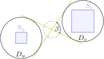
Figure 6: (a) The set of possible directions between two unrelated nodes $\color[rgb]{0.75,0.30,0.15}u$ and $\color[rgb]{0.75,0.30,0.15}v$. (b) The set of possible directions between well-separated pairs is small.

Observation 4.1.

Let $\color[rgb]{0.75,0.30,0.15}u$ and $\color[rgb]{0.75,0.30,0.15}v$ be two unrelated nodes of $\color[rgb]{0.75,0.30,0.15}T$, and let $\color[rgb]{0.75,0.30,0.15}\underline{u}$ be a descendant of $\color[rgb]{0.75,0.30,0.15}u$ and $\color[rgb]{0.75,0.30,0.15}\underline{v}$ be a descendant of $\color[rgb]{0.75,0.30,0.15}v$. Then $\color[rgb]{0.75,0.30,0.15}\Phi_{\underline{u}\underline{v}}\subseteq\Phi_{uv}$.

Proof.

This is immediate, because $\color[rgb]{0.75,0.30,0.15}S_{\underline{u}}\subseteq S_{u}$ and $\color[rgb]{0.75,0.30,0.15}S_{\underline{v}}\subseteq S_{v}$. ∎

Observation 4.2.

If $\color[rgb]{0.75,0.30,0.15}u$ and $\color[rgb]{0.75,0.30,0.15}v$ are two nodes of $\color[rgb]{0.75,0.30,0.15}T$ such that $\color[rgb]{0.75,0.30,0.15}\{u,v\}$ is $\color[rgb]{0.75,0.30,0.15}\varepsilon$-well-separated, then $\color[rgb]{0.75,0.30,0.15}|\Phi_{uv}|\leq 8\varepsilon$.

Proof.

Let $\color[rgb]{0.75,0.30,0.15}d:=|c_{u}c_{v}|$, $\color[rgb]{0.75,0.30,0.15}D_{u}$ be the disk around $\color[rgb]{0.75,0.30,0.15}c_{u}$ with radius $\color[rgb]{0.75,0.30,0.15}\varepsilon d$, and $\color[rgb]{0.75,0.30,0.15}D_{v}$ the disk around $\color[rgb]{0.75,0.30,0.15}c_{v}$ with the same radius. By well-separation, $\color[rgb]{0.75,0.30,0.15}S_{u}\subseteq D_{u}$ and $\color[rgb]{0.75,0.30,0.15}S_{v}\subseteq D_{v}$. Let $\color[rgb]{0.75,0.30,0.15}\beta$ be the angle between the diagonal bitangents of $\color[rgb]{0.75,0.30,0.15}D_{u}$ and $\color[rgb]{0.75,0.30,0.15}D_{v}$. Then $\color[rgb]{0.75,0.30,0.15}|\Phi_{uv}|\leq\beta$, and $\color[rgb]{0.75,0.30,0.15}\beta=2\arcsin(\varepsilon d/\frac{1}{2}d)=2\arcsin(2\varepsilon)\leq 8\varepsilon,$ as claimed. Figure 6 illustrates this. ∎

For a number $\color[rgb]{0.75,0.30,0.15}\phi\in[0,2\pi[$ we define $\color[rgb]{0.75,0.30,0.15}\Phi_{\phi}:=\{\psi\bmod 2\pi\mid\psi\in[\phi-\varepsilon/2,\phi+\varepsilon/2]\}$, i.e., the set of all directions that differ from $\color[rgb]{0.75,0.30,0.15}\phi$ by at most $\color[rgb]{0.75,0.30,0.15}\varepsilon/2$. We say that an ordered pair $\color[rgb]{0.75,0.30,0.15}(u,v)$ of nodes has direction $\color[rgb]{0.75,0.30,0.15}\phi$ if $\color[rgb]{0.75,0.30,0.15}\Phi_{uv}\cap\Phi_{\phi}\neq\emptyset$. We also say that a pair of points $\color[rgb]{0.75,0.30,0.15}(p,q)$ has direction $\color[rgb]{0.75,0.30,0.15}\phi$ if the corresponding pair in the WSPD has direction $\color[rgb]{0.75,0.30,0.15}\phi$. The same definition also applies to an edge. For a given point $\color[rgb]{0.75,0.30,0.15}p$ in the plane, we define the $\color[rgb]{0.75,0.30,0.15}\varepsilon$-cone $\color[rgb]{0.75,0.30,0.15}\mathcal{C}_{\phi}(p)$ as the cone with apex $\color[rgb]{0.75,0.30,0.15}p$ and opening angle $\color[rgb]{0.75,0.30,0.15}\varepsilon$ centered around the direction $\color[rgb]{0.75,0.30,0.15}\phi$.

4.1 Constructing a Supergraph of the EMST

In the following, we abbreviate $\color[rgb]{0.75,0.30,0.15}\mathcal{P}:=\operatorname{\texttt{wspd}}(T)$. The goal of this section is to construct a graph $\color[rgb]{0.75,0.30,0.15}H$ with vertex set $\color[rgb]{0.75,0.30,0.15}P$ and $\color[rgb]{0.75,0.30,0.15}O(n)$ edges, such that $\color[rgb]{0.75,0.30,0.15}\operatorname{emst}(P)\subseteq H$. It is well known that if we take the graph $\color[rgb]{0.75,0.30,0.15}H^{\prime}$ on $\color[rgb]{0.75,0.30,0.15}P$ with edge set $\color[rgb]{0.75,0.30,0.15}E:=\{e_{uv}\mid\{u,v\}\in\mathcal{P}\}$, where each $\color[rgb]{0.75,0.30,0.15}e_{uv}$ connects the bichromatic closest pair for $\color[rgb]{0.75,0.30,0.15}P_{u}$ and $\color[rgb]{0.75,0.30,0.15}P_{v}$, then $\color[rgb]{0.75,0.30,0.15}H^{\prime}$ contains $\color[rgb]{0.75,0.30,0.15}\operatorname{emst}(P)$ and has $\color[rgb]{0.75,0.30,0.15}O(n)$ edges [26]. However, as defined, it is not clear how to find $\color[rgb]{0.75,0.30,0.15}H^{\prime}$ in linear time. There are several major obstacles. Firstly, even though the tree $\color[rgb]{0.75,0.30,0.15}T$ has $\color[rgb]{0.75,0.30,0.15}O(n)$ nodes, it could be that $\color[rgb]{0.75,0.30,0.15}\sum_{u\in T}|P_{u}|=\Omega(n^{2})$. Secondly, even if the total size of all $\color[rgb]{0.75,0.30,0.15}P_{u}$’s was $\color[rgb]{0.75,0.30,0.15}O(n)$, we still need to find bichromatic closest pairs for all pairs in $\color[rgb]{0.75,0.30,0.15}\mathcal{P}$. Thus, a large set $\color[rgb]{0.75,0.30,0.15}P_{u}$ might appear in many pairs of $\color[rgb]{0.75,0.30,0.15}\mathcal{P}$, making the total problem size superlinear. Thirdly, we need to actually solve the bichromatic closest pair problems. A straightforward solution to find the bichromatic closest pair for sets $\color[rgb]{0.75,0.30,0.15}R$ and $\color[rgb]{0.75,0.30,0.15}B$ with sizes $\color[rgb]{0.75,0.30,0.15}r$ and $\color[rgb]{0.75,0.30,0.15}b$ would take time $\color[rgb]{0.75,0.30,0.15}O((r+b)\log(\min(r,b))$, by computing the Voronoi diagram for the smaller set and locating all points from the other set in it. We need to find a way to do it in linear time.

To address these problems, we actually construct a slightly larger graph $\color[rgb]{0.75,0.30,0.15}H$, by partitioning the pairs in $\color[rgb]{0.75,0.30,0.15}\mathcal{P}$ according to their direction. More precisely, let $\color[rgb]{0.75,0.30,0.15}Y=\{0,\varepsilon,2\varepsilon,\ldots,(l-1)\varepsilon\}$ be a set of $\color[rgb]{0.75,0.30,0.15}l$ numbers, where we assume that $\color[rgb]{0.75,0.30,0.15}l=2\pi/\varepsilon$ is an integer. For every $\color[rgb]{0.75,0.30,0.15}\phi\in Y$, we construct a graph $\color[rgb]{0.75,0.30,0.15}H_{\phi}$ with $\color[rgb]{0.75,0.30,0.15}O(n)$ edges and then let $\color[rgb]{0.75,0.30,0.15}H=\bigcup_{\phi\in Y}H_{\phi}$. Given $\color[rgb]{0.75,0.30,0.15}\phi\in Y$, the graph $\color[rgb]{0.75,0.30,0.15}H_{\phi}$ is constructed in three steps:

1. For every node $\color[rgb]{0.75,0.30,0.15}u\in T$, select a subset $\color[rgb]{0.75,0.30,0.15}Z_{u}\subseteq P_{u}$, such that $\color[rgb]{0.75,0.30,0.15}\sum_{u\in T}|Z_{u}|=O(n)$, and such that $\color[rgb]{0.75,0.30,0.15}\{\{p,q\}\mid p\in Z_{u},q\in Z_{v},\{u,v\}\in\mathcal{P}\}$ still contains all edges of $\color[rgb]{0.75,0.30,0.15}\operatorname{emst}(P)$ with orientation $\color[rgb]{0.75,0.30,0.15}\phi$. This addresses the first problem by making the total set size linear.

2. Find a subset $\color[rgb]{0.75,0.30,0.15}\mathcal{P}^{\prime}\subseteq\mathcal{P}$, such that each $\color[rgb]{0.75,0.30,0.15}u\in T$ appears in $\color[rgb]{0.75,0.30,0.15}O(1)$ pairs of $\color[rgb]{0.75,0.30,0.15}\mathcal{P}^{\prime}$, and the set $\color[rgb]{0.75,0.30,0.15}\{\{p,q\}\mid p\in Z_{u},q\in Z_{v},\{u,v\}\in\mathcal{P}^{\prime}\}$ contains all edges of $\color[rgb]{0.75,0.30,0.15}\operatorname{emst}(P)$ with orientation $\color[rgb]{0.75,0.30,0.15}\phi$. In particular, we choose for every node $\color[rgb]{0.75,0.30,0.15}u\in T$ a subset $\color[rgb]{0.75,0.30,0.15}\mathcal{P}_{u}\subseteq\mathcal{P}$ such that $\color[rgb]{0.75,0.30,0.15}\mathcal{P}^{\prime}=\bigcup_{u\in T}\mathcal{P}_{u}$, each pair in $\color[rgb]{0.75,0.30,0.15}\mathcal{P}_{u}$ contains $\color[rgb]{0.75,0.30,0.15}u$, and $\color[rgb]{0.75,0.30,0.15}|\mathcal{P}_{u}|=O(1)$. This addresses the second problem by ensuring that every set appears in $\color[rgb]{0.75,0.30,0.15}O(1)$ pairs.

3. For every pair $\color[rgb]{0.75,0.30,0.15}\{u,v\}\in\mathcal{P}^{\prime}$, we include in $\color[rgb]{0.75,0.30,0.15}H_{\phi}$ the edge $\color[rgb]{0.75,0.30,0.15}pq$ such that $\color[rgb]{0.75,0.30,0.15}\{p,q\}$ is the closest pair in $\color[rgb]{0.75,0.30,0.15}Z_{u}\otimes Z_{v}$ (i.e., $\color[rgb]{0.75,0.30,0.15}\{p,q\}=\operatorname{argmin}_{\{p^{\prime},q^{\prime}\}\in Z_{u}\otimes Z_{v}}|p^{\prime}q^{\prime}|$). Here we actually solve all the bichromatic closest pair problems.

Clearly, $\color[rgb]{0.75,0.30,0.15}H_{\phi}$ has $\color[rgb]{0.75,0.30,0.15}O(n)$ edges, and we will show that $\color[rgb]{0.75,0.30,0.15}H$ is indeed a supergraph of $\color[rgb]{0.75,0.30,0.15}\operatorname{emst}(P)$. Our strategy of subdividing the edges according to their orientation goes back to Yao, who used a similar scheme to find EMSTs in higher dimensions [51].

Step 1: Finding the $\color[rgb]{0.75,0.30,0.15}Z_{u}$’s.

Recall that we fixed a direction $\color[rgb]{0.75,0.30,0.15}\phi\in Y$. Take the set $\color[rgb]{0.75,0.30,0.15}\mathcal{P}_{\phi}\subseteq\operatorname{\texttt{wspd}}(T)$ of pairs with direction $\color[rgb]{0.75,0.30,0.15}\phi$. For a pair $\color[rgb]{0.75,0.30,0.15}\pi\in\mathcal{P}_{\phi}$, we write $\color[rgb]{0.75,0.30,0.15}(u,v)$ for the tuple such that $\color[rgb]{0.75,0.30,0.15}\pi=\{u,v\}$ and $\color[rgb]{0.75,0.30,0.15}c_{u}$ comes before $\color[rgb]{0.75,0.30,0.15}c_{v}$ in direction $\color[rgb]{0.75,0.30,0.15}\phi$, it is a directed pair in $\color[rgb]{0.75,0.30,0.15}\mathcal{P}_{\phi}$. Call a node $\color[rgb]{0.75,0.30,0.15}u$ of $\color[rgb]{0.75,0.30,0.15}T$ full if either (i) $\color[rgb]{0.75,0.30,0.15}u$ is the root; (ii) $\color[rgb]{0.75,0.30,0.15}u$ is a non-empty leaf; or (iii) $\color[rgb]{0.75,0.30,0.15}\mathcal{P_{\phi}}$ has a directed pair $\color[rgb]{0.75,0.30,0.15}(u,v)$. Let $\color[rgb]{0.75,0.30,0.15}T^{\prime}$ be the tree obtained from $\color[rgb]{0.75,0.30,0.15}T$ by connecting every full node to its closest full ancestor, and by removing the other nodes. We can compute $\color[rgb]{0.75,0.30,0.15}T^{\prime}$ in linear time through a post-order traversal. Now, for every leaf $\color[rgb]{0.75,0.30,0.15}v$ of $\color[rgb]{0.75,0.30,0.15}T^{\prime}$, put the point $\color[rgb]{0.75,0.30,0.15}p\in P_{v}$ into the sets $\color[rgb]{0.75,0.30,0.15}Z_{u}$, where $\color[rgb]{0.75,0.30,0.15}u$ is one the $\color[rgb]{0.75,0.30,0.15}k$ closest ancestors of $\color[rgb]{0.75,0.30,0.15}v$ in $\color[rgb]{0.75,0.30,0.15}T^{\prime}$. Repeat this procedure, while changing property (iii) above so that $\color[rgb]{0.75,0.30,0.15}\mathcal{P}_{\phi}$ has a directed pair $\color[rgb]{0.75,0.30,0.15}(v,u)$. This takes linear time, and $\color[rgb]{0.75,0.30,0.15}\sum_{u\in T}|Z_{u}|=O(n)$. Intuitively, $\color[rgb]{0.75,0.30,0.15}Z_{u}$ contains those points of $\color[rgb]{0.75,0.30,0.15}P_{u}$ that are sufficiently on the outside of the point set in direction $\color[rgb]{0.75,0.30,0.15}\phi$. Figure 7 shows an example.

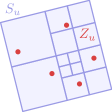
Figure 7: (a) A node $\color[rgb]{0.75,0.30,0.15}u$ in the quadtree, with $\color[rgb]{0.75,0.30,0.15}|P_{u}|=8$. (b) The relevant wspd-pairs (in green) for the points in $\color[rgb]{0.75,0.30,0.15}P_{u}$ with direction $\color[rgb]{0.75,0.30,0.15}\phi$ (up). There are also wspd-pairs between $\color[rgb]{0.75,0.30,0.15}u$ and other nodes above and below it. (c) For $\color[rgb]{0.75,0.30,0.15}k=1$, $\color[rgb]{0.75,0.30,0.15}Z_{u}$ contains those $\color[rgb]{0.75,0.30,0.15}p\in P_{u}$ for which the lowest wspd-pair in the tree $\color[rgb]{0.75,0.30,0.15}T^{\prime}$ that involves $\color[rgb]{0.75,0.30,0.15}p$ contains $\color[rgb]{0.75,0.30,0.15}u$. In other words, $\color[rgb]{0.75,0.30,0.15}Z_{u}$ has the points that do not have a green edge in both directions in (b).

Variants of the following claim have appeared several times before [1, 51].

Claim 4.3.

Let $\color[rgb]{0.75,0.30,0.15}p\in P$, and let $\color[rgb]{0.75,0.30,0.15}\mathcal{C}^{+}_{\phi}(p)$ denote the cone with apex $\color[rgb]{0.75,0.30,0.15}p$ and opening angle $\color[rgb]{0.75,0.30,0.15}17\varepsilon$ centered around $\color[rgb]{0.75,0.30,0.15}\phi$. Suppose that $\color[rgb]{0.75,0.30,0.15}pq$ is an edge of $\color[rgb]{0.75,0.30,0.15}\operatorname{emst}(P)$ and $\color[rgb]{0.75,0.30,0.15}q\in\mathcal{C}^{+}_{\phi}(p)$. Then $\color[rgb]{0.75,0.30,0.15}q$ is the nearest neighbor of $\color[rgb]{0.75,0.30,0.15}p$ in $\color[rgb]{0.75,0.30,0.15}\mathcal{C}^{+}_{\phi}(p)\cap P$.

Proof.

If $\color[rgb]{0.75,0.30,0.15}pq$ is an edge of $\color[rgb]{0.75,0.30,0.15}\operatorname{emst}(P)$, then the lune $\color[rgb]{0.75,0.30,0.15}L$ defined by $\color[rgb]{0.75,0.30,0.15}p$ and $\color[rgb]{0.75,0.30,0.15}q$ contains no point of $\color[rgb]{0.75,0.30,0.15}P$ [3]. Since the opening angle of $\color[rgb]{0.75,0.30,0.15}\mathcal{C}^{+}_{\phi}(p)$ is at most $\color[rgb]{0.75,0.30,0.15}\pi/3$, for $\color[rgb]{0.75,0.30,0.15}\varepsilon$ small enough, the intersection of $\color[rgb]{0.75,0.30,0.15}\mathcal{C}^{+}_{\phi}(p)$ with $\color[rgb]{0.75,0.30,0.15}L$ equals the intersection of $\color[rgb]{0.75,0.30,0.15}\mathcal{C}^{+}_{\phi}(p)$ with the disk around $\color[rgb]{0.75,0.30,0.15}p$ of radius $\color[rgb]{0.75,0.30,0.15}|pq|$. Hence, $\color[rgb]{0.75,0.30,0.15}q$ must be the nearest neighbor of $\color[rgb]{0.75,0.30,0.15}p$ in $\color[rgb]{0.75,0.30,0.15}\mathcal{C}^{+}_{\phi}(p)\cap P$. ∎

Lemma 4.4.

Let $\color[rgb]{0.75,0.30,0.15}pq$ be an edge of $\color[rgb]{0.75,0.30,0.15}\operatorname{emst}(P)$ with direction $\color[rgb]{0.75,0.30,0.15}\phi$, and let $\color[rgb]{0.75,0.30,0.15}\{u,v\}$ be the corresponding wspd-pair. Then $\color[rgb]{0.75,0.30,0.15}\{p,q\}\in Z_{u}\otimes Z_{v}$.

Proof.

Let $\color[rgb]{0.75,0.30,0.15}w$ be the leaf for $\color[rgb]{0.75,0.30,0.15}p$, and suppose for contradiction that $\color[rgb]{0.75,0.30,0.15}p\notin Z_{u}$, i.e., $\color[rgb]{0.75,0.30,0.15}u$ is not among the $\color[rgb]{0.75,0.30,0.15}k$ closest ancestors of $\color[rgb]{0.75,0.30,0.15}w$ in $\color[rgb]{0.75,0.30,0.15}T^{\prime}$. This means there exists a sequence $\color[rgb]{0.75,0.30,0.15}u_{1},u_{2},\ldots,u_{k},u$ of $\color[rgb]{0.75,0.30,0.15}k+1$ distinct ancestors of $\color[rgb]{0.75,0.30,0.15}w$, such that each node is an ancestor of all previous nodes and such there are well-separated pairs $\color[rgb]{0.75,0.30,0.15}\{u_{1},v_{1}\},\{u_{2},v_{2}\},\ldots,\{u_{k},v_{k}\}\in\mathcal{P}_{\phi}$.

Let $\color[rgb]{0.75,0.30,0.15}\mathcal{C}^{+}_{\phi}(p)$ be the cone with apex $\color[rgb]{0.75,0.30,0.15}p$ and opening angle $\color[rgb]{0.75,0.30,0.15}17\varepsilon$ centered around $\color[rgb]{0.75,0.30,0.15}\phi$. By Observation 4.2, we have $\color[rgb]{0.75,0.30,0.15}S_{v},S_{v_{1}},\ldots,S_{v_{k}}\subseteq\mathcal{C}^{+}_{\phi}(p)$. Furthermore, since $\color[rgb]{0.75,0.30,0.15}\{u,v\}$ is well-separated, $\color[rgb]{0.75,0.30,0.15}d(u,v)\geq|S_{u}|/\varepsilon$. Now Claim 2.4 implies that there are squares $\color[rgb]{0.75,0.30,0.15}R_{u_{1}}$, $\color[rgb]{0.75,0.30,0.15}R_{v_{1}}$ such that (i) $\color[rgb]{0.75,0.30,0.15}S_{u_{1}}\subseteq R_{u_{1}}\subseteq S_{u_{2}}$ and $\color[rgb]{0.75,0.30,0.15}S_{v_{1}}\subseteq R_{v_{1}}$; (ii) $\color[rgb]{0.75,0.30,0.15}|R_{u_{1}}|=|R_{v_{1}}|$; and (iii) $\color[rgb]{0.75,0.30,0.15}d(R_{u_{1}},R_{v_{1}})\leq 2|R_{u_{1}}|/\varepsilon$. This means that

$$\color[rgb]{0.75,0.30,0.15}d(p,P_{v_{1}})\leq 2(1+1/\varepsilon)|R_{u_{1}}|\leq 2(1+1/\varepsilon)|S_{u_{2}}|\leq 2(1+1/\varepsilon)|S_{u}|/2^{k-1},$$

where in the first inequality we bounded the distance between any point in $\color[rgb]{0.75,0.30,0.15}R_{u_{1}}$ and any point in $\color[rgb]{0.75,0.30,0.15}R_{v_{1}}$ by the distance between the squares plus their diameter (since we do not know where the points lie inside the squares). The second inequality comes from $\color[rgb]{0.75,0.30,0.15}R_{u_{1}}\subseteq S_{u_{2}}$ and the third inequality is due to the fact that $\color[rgb]{0.75,0.30,0.15}S_{u_{2}}$ lies at least $\color[rgb]{0.75,0.30,0.15}k-1$ levels below $\color[rgb]{0.75,0.30,0.15}S_{u}$ in $\color[rgb]{0.75,0.30,0.15}T^{\prime}$.

Since $\color[rgb]{0.75,0.30,0.15}2(1+1/\varepsilon)/2^{k-1}<1/\varepsilon$ for $\color[rgb]{0.75,0.30,0.15}k\geq 3$ and since $\color[rgb]{0.75,0.30,0.15}d(u,v)\geq|S_{u}|/\varepsilon$, this contradicts the fact that $\color[rgb]{0.75,0.30,0.15}q$ is the nearest neighbor of $\color[rgb]{0.75,0.30,0.15}p$ inside $\color[rgb]{0.75,0.30,0.15}\mathcal{C}^{+}_{\phi}(p)$ (Claim 4.3). Thus, $\color[rgb]{0.75,0.30,0.15}p$ must lie in $\color[rgb]{0.75,0.30,0.15}Z_{u}$. A symmetric argument shows $\color[rgb]{0.75,0.30,0.15}q\in Z_{v}$. ∎

Step 2: Finding the $\color[rgb]{0.75,0.30,0.15}\mathcal{P}_{u}$’s.

For every node $\color[rgb]{0.75,0.30,0.15}u\in T$, we include in $\color[rgb]{0.75,0.30,0.15}\mathcal{P}_{u}$ the $\color[rgb]{0.75,0.30,0.15}k$ shortest pairs in direction $\color[rgb]{0.75,0.30,0.15}\phi$, i.e., the pairs $\color[rgb]{0.75,0.30,0.15}\{u,v\}\in\operatorname{\texttt{wspd}}(T)$ such that (i) $\color[rgb]{0.75,0.30,0.15}c_{v}$ is contained in the $\color[rgb]{0.75,0.30,0.15}\varepsilon$-cone $\color[rgb]{0.75,0.30,0.15}\mathcal{C}_{\phi}(c_{u})$ with apex $\color[rgb]{0.75,0.30,0.15}c_{u}$ centered around direction $\color[rgb]{0.75,0.30,0.15}\phi$; and (ii) there are less than $\color[rgb]{0.75,0.30,0.15}k$ pairs $\color[rgb]{0.75,0.30,0.15}\{u,v^{\prime}\}\in\operatorname{\texttt{wspd}}(T)$ that fulfill (i) and have $\color[rgb]{0.75,0.30,0.15}|c_{u}c_{v^{\prime}}|<|c_{u}c_{v}|$. Since $\color[rgb]{0.75,0.30,0.15}k$ is constant, the $\color[rgb]{0.75,0.30,0.15}\mathcal{P}_{u}$’s can be constructed in total linear time. Even though each $\color[rgb]{0.75,0.30,0.15}\mathcal{P}_{u}$ contains a constant number of elements, a node might still appear in many such sets, so we further prune the pairs: by examining the $\color[rgb]{0.75,0.30,0.15}\mathcal{P}_{u}$’s, determine for each $\color[rgb]{0.75,0.30,0.15}v\in T$ the set $\color[rgb]{0.75,0.30,0.15}\mathcal{Q}_{v}=\{u\in T\mid v\in\mathcal{P}_{u}\}$. For each $\color[rgb]{0.75,0.30,0.15}\mathcal{Q}_{v}$, find the $\color[rgb]{0.75,0.30,0.15}k$ closest neighbors (measured by the distance between their center points) of $\color[rgb]{0.75,0.30,0.15}v$ in $\color[rgb]{0.75,0.30,0.15}\mathcal{Q}_{v}$, and for all other $\color[rgb]{0.75,0.30,0.15}\mathcal{P}_{u}$’s remove the corresponding pairs $\color[rgb]{0.75,0.30,0.15}\{u,v\}$. Now each node appears in only a constant number of pairs of $\color[rgb]{0.75,0.30,0.15}\mathcal{P}^{\prime}=\bigcup_{u\in T}\mathcal{P}_{u}$.

Lemma 4.5.

Let $\color[rgb]{0.75,0.30,0.15}pq$ be an edge of $\color[rgb]{0.75,0.30,0.15}\operatorname{emst}(P)$ with orientation $\color[rgb]{0.75,0.30,0.15}\phi$, and let $\color[rgb]{0.75,0.30,0.15}\{u,v\}$ be the corresponding wspd-pair. Then $\color[rgb]{0.75,0.30,0.15}\{u,v\}\in\mathcal{P}_{u}$.

Proof.

We show that $\color[rgb]{0.75,0.30,0.15}v$ is among the $\color[rgb]{0.75,0.30,0.15}k$ closest neighbors of $\color[rgb]{0.75,0.30,0.15}u$ in direction $\color[rgb]{0.75,0.30,0.15}\phi$, a symmetric argument shows that $\color[rgb]{0.75,0.30,0.15}u$ is among the $\color[rgb]{0.75,0.30,0.15}k$ closest neighbors of $\color[rgb]{0.75,0.30,0.15}v$ in direction $\color[rgb]{0.75,0.30,0.15}-\phi$. We may assume that $\color[rgb]{0.75,0.30,0.15}|c_{u}c_{v}|=1$. Suppose that $\color[rgb]{0.75,0.30,0.15}\{u,v\}$ is not among the $\color[rgb]{0.75,0.30,0.15}k$ shortest pairs in direction $\color[rgb]{0.75,0.30,0.15}\phi$. Then there is a set $\color[rgb]{0.75,0.30,0.15}W$ of $\color[rgb]{0.75,0.30,0.15}k$ nodes of $\color[rgb]{0.75,0.30,0.15}T$ such that for all $\color[rgb]{0.75,0.30,0.15}w\in W$ we have (i) $\color[rgb]{0.75,0.30,0.15}c_{w}\in\mathcal{C}_{\phi}(c_{u})$; (ii) $\color[rgb]{0.75,0.30,0.15}|c_{u}c_{w}|<1$; and (iii) $\color[rgb]{0.75,0.30,0.15}\{u,w\}\in\operatorname{\texttt{wspd}}(T)$. By Claim 2.4, there exists for every $\color[rgb]{0.75,0.30,0.15}w\in W$ a pair of squares $\color[rgb]{0.75,0.30,0.15}R_{u}(w),R_{w}$ such that $\color[rgb]{0.75,0.30,0.15}S_{u}\subseteq R_{u}(w)$, $\color[rgb]{0.75,0.30,0.15}S_{w}\subseteq R_{w}$ and $\color[rgb]{0.75,0.30,0.15}|R_{u}(w)|=|R_{w}|\leq 2\varepsilon d(R_{u}(w),R_{w})\leq 2\varepsilon$.

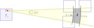
Figure 8: All squares $\color[rgb]{0.75,0.30,0.15}R_{w}$ intersect the region $\color[rgb]{0.75,0.30,0.15}A$.

Let $\color[rgb]{0.75,0.30,0.15}\mathcal{C}^{+}_{\phi}(p)$ be the cone with apex $\color[rgb]{0.75,0.30,0.15}p$ and opening angle $\color[rgb]{0.75,0.30,0.15}17\varepsilon$ centered around $\color[rgb]{0.75,0.30,0.15}\phi$. By Observation 4.2, $\color[rgb]{0.75,0.30,0.15}S_{w}\subseteq\mathcal{C}^{+}_{\phi}(p)$ for all $\color[rgb]{0.75,0.30,0.15}w\in W$. Furthermore, every $\color[rgb]{0.75,0.30,0.15}S_{w}$ contains a point at distance at most $\color[rgb]{0.75,0.30,0.15}1+\varepsilon$ from $\color[rgb]{0.75,0.30,0.15}p$, because $\color[rgb]{0.75,0.30,0.15}|c_{w}p|\leq|c_{w}c_{u}|+|c_{u}p|\leq 1+\varepsilon$. Also, by Claim 4.3, every $\color[rgb]{0.75,0.30,0.15}S_{w}$ contains a point at distance at least $\color[rgb]{0.75,0.30,0.15}|pq|\geq|c_{u}c_{v}|-|c_{u}p|-|qc_{v}|\geq 1-2\varepsilon$ from $\color[rgb]{0.75,0.30,0.15}p$. Thus, since $\color[rgb]{0.75,0.30,0.15}d(R_{u}(w),R_{w})\leq 2|R_{w}|/\varepsilon$ by Claim 2.4 and $\color[rgb]{0.75,0.30,0.15}d(R_{u}(w),R_{w})\geq 1-2\varepsilon-2|R_{w}|$, we get $\color[rgb]{0.75,0.30,0.15}|R_{w}|\geq\varepsilon/8$, for $\color[rgb]{0.75,0.30,0.15}\varepsilon$ small enough. However, this implies that $\color[rgb]{0.75,0.30,0.15}W$ has only a constant number of squares: all $\color[rgb]{0.75,0.30,0.15}S_{w}$ (and hence all $\color[rgb]{0.75,0.30,0.15}R_{w}$) intersect the annular segment $\color[rgb]{0.75,0.30,0.15}A$ inside $\color[rgb]{0.75,0.30,0.15}\mathcal{C}^{+}_{\phi}(p)$ with inner radius $\color[rgb]{0.75,0.30,0.15}1-2\varepsilon$ and outer radius $\color[rgb]{0.75,0.30,0.15}1+\varepsilon$ (see Figure 8). All $\color[rgb]{0.75,0.30,0.15}w\in W$ are unrelated, since they are paired with $\color[rgb]{0.75,0.30,0.15}u$ in $\color[rgb]{0.75,0.30,0.15}\operatorname{\texttt{wspd}}(T)$. Furthermore, the set $\color[rgb]{0.75,0.30,0.15}A$ has diameter $\color[rgb]{0.75,0.30,0.15}O(\varepsilon)$. If $\color[rgb]{0.75,0.30,0.15}w\in W$ is a compressed child, then $\color[rgb]{0.75,0.30,0.15}R_{w}$ is contained in the parent of $\color[rgb]{0.75,0.30,0.15}w$ and intersects no other $\color[rgb]{0.75,0.30,0.15}S_{w^{\prime}}$, for $\color[rgb]{0.75,0.30,0.15}w^{\prime}\in W$. Otherwise, $\color[rgb]{0.75,0.30,0.15}|S_{w}|\geq|R_{w}|/2$. Thus, if we assign to each compressed child $\color[rgb]{0.75,0.30,0.15}w\in W$ the square $\color[rgb]{0.75,0.30,0.15}R_{w}$ and to each other node $\color[rgb]{0.75,0.30,0.15}w\in W$ the square $\color[rgb]{0.75,0.30,0.15}S_{w}$, we get a collection of $\color[rgb]{0.75,0.30,0.15}k$ disjoint squares that meet $\color[rgb]{0.75,0.30,0.15}A$ and each have diameter $\color[rgb]{0.75,0.30,0.15}\Omega(\varepsilon)$. Since $\color[rgb]{0.75,0.30,0.15}A$ has diameter $\color[rgb]{0.75,0.30,0.15}O(\varepsilon)$, there can be only a constant number of such squares, so choosing $\color[rgb]{0.75,0.30,0.15}k$ large enough leads to a contradiction. ∎

Step 3: Finding the Nearest Neighbors.

Unlike in the previous steps, the algorithm for Step 3 is a bit involved, so we switch the order and begin by showing correctness.

Lemma 4.6.

Let $\color[rgb]{0.75,0.30,0.15}pq$ be an edge of $\color[rgb]{0.75,0.30,0.15}\operatorname{emst}(P)$ with direction $\color[rgb]{0.75,0.30,0.15}\phi$ and let $\color[rgb]{0.75,0.30,0.15}\{u,v\}$ be the corresponding wspd-pair. Then $\color[rgb]{0.75,0.30,0.15}\{p,q\}$ is the closest pair in $\color[rgb]{0.75,0.30,0.15}Z_{u}\otimes Z_{v}$.

Proof.

By Lemma 4.4, we have $\color[rgb]{0.75,0.30,0.15}\{p,q\}\in Z_{u}\otimes Z_{v}$. Furthermore, the cut property of minimum spanning trees implies that $\color[rgb]{0.75,0.30,0.15}pq\in\operatorname{emst}(Z_{u}\cup Z_{v})$. Since $\color[rgb]{0.75,0.30,0.15}\{u,v\}$ is well-separated, we have

$$\max_{\{p^{\prime},q^{\prime}\}\in Z_{u}\otimes Z_{u}\cup Z_{v}\otimes Z_{v}}|p^{\prime}q^{\prime}|<\min_{\{p^{\prime},q^{\prime}\}\in Z_{u}\otimes Z_{v}}|p^{\prime}q^{\prime}|.$$ (1)

Now consider an execution of Kruskal’s MST algorithm on $\color[rgb]{0.75,0.30,0.15}Z_{u}\cup Z_{v}$ [22, Chapter 23.2]. Let $\color[rgb]{0.75,0.30,0.15}\{p^{\prime},q^{\prime}\}$ be the closest pair in $\color[rgb]{0.75,0.30,0.15}Z_{u}\otimes Z_{v}$. By $\color[rgb]{0.75,0.30,0.15}(\ref{equ:order})$, the algorithm considers $\color[rgb]{0.75,0.30,0.15}p^{\prime}q^{\prime}$ only after processing all edges in $\color[rgb]{0.75,0.30,0.15}Z_{u}\otimes Z_{u}\cup Z_{v}\otimes Z_{v}$. Hence, at that point the sets $\color[rgb]{0.75,0.30,0.15}Z_{u}$ and $\color[rgb]{0.75,0.30,0.15}Z_{v}$ are each contained in a connected component of the partial spanning tree, and $\color[rgb]{0.75,0.30,0.15}\operatorname{emst}(Z_{u}\cup Z_{v})$ can have at most one edge from $\color[rgb]{0.75,0.30,0.15}Z_{u}\otimes Z_{v}$. Hence, it follows that $\color[rgb]{0.75,0.30,0.15}\{p,q\}=\{p^{\prime},q^{\prime}\}$, as claimed. ∎

We now describe the algorithm. For ease of exposition, we take $\color[rgb]{0.75,0.30,0.15}\phi=\pi/2$ (i.e., we assume that $\color[rgb]{0.75,0.30,0.15}P$ is rotated so that $\color[rgb]{0.75,0.30,0.15}\phi$ points in the positive $\color[rgb]{0.75,0.30,0.15}y$-direction). Note that now the squares are not generally axis-aligned anymore, but this will be no problem. Given a point $\color[rgb]{0.75,0.30,0.15}p\in\mathbb{R}^{2}$, we define the four directional cones $\color[rgb]{0.75,0.30,0.15}\mathcal{C}_{\leftarrow}(p)$,$\color[rgb]{0.75,0.30,0.15}\mathcal{C}_{\uparrow}(p)$, $\color[rgb]{0.75,0.30,0.15}\mathcal{C}_{\rightarrow}(p)$, and $\color[rgb]{0.75,0.30,0.15}\mathcal{C}_{\downarrow}(p)$ as the leftward, upward, rightward and downward cones with apex $\color[rgb]{0.75,0.30,0.15}p$ and opening angle $\color[rgb]{0.75,0.30,0.15}\pi/2$. The directional cones subdivide the plane into four disjoint sectors. We will also need the extended rightward cone $\color[rgb]{0.75,0.30,0.15}\mathcal{C}_{\rightarrow}^{+}(p)$ with apex $\color[rgb]{0.75,0.30,0.15}p$ and opening angle $\color[rgb]{0.75,0.30,0.15}\pi/2+16\varepsilon$.

Claim 4.7.

Let $\color[rgb]{0.75,0.30,0.15}(u,v)$ be a directed pair in $\color[rgb]{0.75,0.30,0.15}\mathcal{P}_{\phi}$, and suppose that $\color[rgb]{0.75,0.30,0.15}\{p,q\}$ with $\color[rgb]{0.75,0.30,0.15}p\in P_{u}$ and $\color[rgb]{0.75,0.30,0.15}q\in P_{v}$ is the closest pair for $\color[rgb]{0.75,0.30,0.15}(u,v)$. Then $\color[rgb]{0.75,0.30,0.15}\mathcal{C}_{\uparrow}(p)\cap P_{u}=\emptyset$ and $\color[rgb]{0.75,0.30,0.15}\mathcal{C}_{\downarrow}(q)\cap P_{v}=\emptyset$.

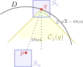
Figure 9: The intersection points of $\color[rgb]{0.75,0.30,0.15}D$ and the boundary of $\color[rgb]{0.75,0.30,0.15}\mathcal{C}_{\downarrow}(q)$ lie outside $\color[rgb]{0.75,0.30,0.15}S_{v}$, so $\color[rgb]{0.75,0.30,0.15}S_{v}\cap\mathcal{C}_{\downarrow}(q)\subseteq D$.

Proof.

We prove the claim for $\color[rgb]{0.75,0.30,0.15}\mathcal{C}_{\downarrow}(q)$, the argument for $\color[rgb]{0.75,0.30,0.15}\mathcal{C}_{\uparrow}(p)$ is symmetric. We may assume that $\color[rgb]{0.75,0.30,0.15}|pq|=1$. By assumption, the unit disk $\color[rgb]{0.75,0.30,0.15}D$ centered at $\color[rgb]{0.75,0.30,0.15}p$ contains no points of $\color[rgb]{0.75,0.30,0.15}P_{v}$, so it suffices to show that $\color[rgb]{0.75,0.30,0.15}\mathcal{C}_{\downarrow}(q)\cap S_{v}\subseteq D$. Since $\color[rgb]{0.75,0.30,0.15}\{u,v\}\in\mathcal{P}_{\phi}$ and by Observation 4.2, the direction of the line $\color[rgb]{0.75,0.30,0.15}\overline{pq}$ differs from $\color[rgb]{0.75,0.30,0.15}\phi$ by at most $\color[rgb]{0.75,0.30,0.15}17\varepsilon$. Therefore, the intersections of the boundaries of $\color[rgb]{0.75,0.30,0.15}\mathcal{C}_{\downarrow}(q)$ and $\color[rgb]{0.75,0.30,0.15}D$ have distance at least $\color[rgb]{0.75,0.30,0.15}\sqrt{2}-O(\varepsilon)$ from $\color[rgb]{0.75,0.30,0.15}q$. However, the pair $\color[rgb]{0.75,0.30,0.15}\{u,v\}$ is well-separated, so all points in $\color[rgb]{0.75,0.30,0.15}P_{v}$ have distance at most $\color[rgb]{0.75,0.30,0.15}\varepsilon$ from $\color[rgb]{0.75,0.30,0.15}q$, which implies the claim; see Figure 9. ∎

Given a set $\color[rgb]{0.75,0.30,0.15}Z_{u}$ for a node $\color[rgb]{0.75,0.30,0.15}u$ of $\color[rgb]{0.75,0.30,0.15}T$, we define the upper chain of $\color[rgb]{0.75,0.30,0.15}Z_{u}$, $\color[rgb]{0.75,0.30,0.15}\operatorname{UC}(Z_{u})$ as follows: remove from $\color[rgb]{0.75,0.30,0.15}Z_{u}$ all points $\color[rgb]{0.75,0.30,0.15}p$ such that $\color[rgb]{0.75,0.30,0.15}\mathcal{C}_{\uparrow}(p)$ contains a point from $\color[rgb]{0.75,0.30,0.15}Z_{u}$ in its interior. Then sort $\color[rgb]{0.75,0.30,0.15}Z_{u}$ by $\color[rgb]{0.75,0.30,0.15}x$-coordinate and connect consecutive points by line segments. All segments of $\color[rgb]{0.75,0.30,0.15}\operatorname{UC}(Z_{u})$ have slopes in $\color[rgb]{0.75,0.30,0.15}[-1,1]$. Similarly, we define the lower chain of $\color[rgb]{0.75,0.30,0.15}Z_{u}$, $\color[rgb]{0.75,0.30,0.15}\operatorname{LC}(Z_{u})$, by requiring the cones $\color[rgb]{0.75,0.30,0.15}\mathcal{C}_{\downarrow}(p)$ for the points in $\color[rgb]{0.75,0.30,0.15}\operatorname{LC}(Z_{u})$ to be empty. The goal now is to compute $\color[rgb]{0.75,0.30,0.15}\operatorname{UC}(Z_{u})$ and $\color[rgb]{0.75,0.30,0.15}\operatorname{LC}(Z_{u})$ for all nodes $\color[rgb]{0.75,0.30,0.15}u$.

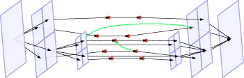
Figure 10: (a) A node $\color[rgb]{0.75,0.30,0.15}u$ with $\color[rgb]{0.75,0.30,0.15}|Z_{u}|=5$, and the relevant part of the quadtree. (b) The graph $\color[rgb]{0.75,0.30,0.15}\Gamma$. Tree edges are black (going right). To avoid clutter, we just show two wspd edges (green, going left).

Define a directed graph $\color[rgb]{0.75,0.30,0.15}\Gamma$ as follows: we create two copies of each vertex $\color[rgb]{0.75,0.30,0.15}u$ in $\color[rgb]{0.75,0.30,0.15}T$, called $\color[rgb]{0.75,0.30,0.15}\texttt{start}(u)$ and $\color[rgb]{0.75,0.30,0.15}\texttt{end}(u)$, and we add a directed edge from $\color[rgb]{0.75,0.30,0.15}\texttt{start}(u)$ to $\color[rgb]{0.75,0.30,0.15}\texttt{end}(u)$ for each such vertex. Furthermore, we replace every edge $\color[rgb]{0.75,0.30,0.15}uv$ of $\color[rgb]{0.75,0.30,0.15}T$ ($\color[rgb]{0.75,0.30,0.15}u$ being the parent of $\color[rgb]{0.75,0.30,0.15}v$) by two edges: one from $\color[rgb]{0.75,0.30,0.15}\texttt{start}(u)$ to $\color[rgb]{0.75,0.30,0.15}\texttt{start}(v)$, and one from $\color[rgb]{0.75,0.30,0.15}\texttt{end}(v)$ to $\color[rgb]{0.75,0.30,0.15}\texttt{end}(u)$. We call these edges the tree-edges. Finally, for every pair $\color[rgb]{0.75,0.30,0.15}\{u,v\}\in\operatorname{\texttt{wspd}}(T)$, where $\color[rgb]{0.75,0.30,0.15}S_{v}$ is wholly contained in the extended rightward cone $\color[rgb]{0.75,0.30,0.15}\mathcal{C}_{\rightarrow}^{+}(c_{u})$, we create a directed edge from $\color[rgb]{0.75,0.30,0.15}\texttt{end}(u)$ to $\color[rgb]{0.75,0.30,0.15}\texttt{start}(v)$. These edges are called wspd-edges. Figure 10 shows a small example.

Claim 4.8.

The graph $\color[rgb]{0.75,0.30,0.15}\Gamma$ is acyclic.

Proof.

Suppose $\color[rgb]{0.75,0.30,0.15}C$ is a cycle in $\color[rgb]{0.75,0.30,0.15}\Gamma$. The tree-edges form an acyclic subgraph, so $\color[rgb]{0.75,0.30,0.15}C$ has at least one wspd-edge. Let $\color[rgb]{0.75,0.30,0.15}e_{1},e_{2},\ldots,e_{z}$ be the sequence of wspd-edges along $\color[rgb]{0.75,0.30,0.15}C$, and let $\color[rgb]{0.75,0.30,0.15}v_{1},\ldots,v_{z}$ be such that the endpoint of $\color[rgb]{0.75,0.30,0.15}e_{i}$ is of the form $\color[rgb]{0.75,0.30,0.15}\texttt{start}(v_{i})$. Finally, write $\color[rgb]{0.75,0.30,0.15}C=e_{1}\rightarrow C_{1}\rightarrow e_{2}\rightarrow C_{2}\rightarrow\cdots\rightarrow e_{z}\rightarrow C_{z}$, where $\color[rgb]{0.75,0.30,0.15}C_{i}$ is the sequence of tree-edges between two consecutive wspd-edges. Each $\color[rgb]{0.75,0.30,0.15}C_{i}$ consists of a (possibly empty) sequence of $\color[rgb]{0.75,0.30,0.15}\texttt{start}-\texttt{start}$ edges, followed by one $\color[rgb]{0.75,0.30,0.15}\texttt{start}-\texttt{end}$ edge and a (possibly empty) sequence of $\color[rgb]{0.75,0.30,0.15}\texttt{end}-\texttt{end}$ edges. Thus, the origin of the next wspd-edge $\color[rgb]{0.75,0.30,0.15}e_{i+1}$ is an end-node for an ancestor or a descendant of $\color[rgb]{0.75,0.30,0.15}v_{i}$ in $\color[rgb]{0.75,0.30,0.15}T$. In either case, by the definition of wspd-edges, it follows that the leftmost point of $\color[rgb]{0.75,0.30,0.15}S_{v_{i+1}}$ lies strictly to the right of the leftmost point of $\color[rgb]{0.75,0.30,0.15}S_{v_{i}}$. Indeed, write $\color[rgb]{0.75,0.30,0.15}e_{i+1}=(u_{i+1},v_{i+1})$. Then $\color[rgb]{0.75,0.30,0.15}S_{v_{i+1}}$ lies strictly to the right of $\color[rgb]{0.75,0.30,0.15}S_{u_{i+1}}$, because $\color[rgb]{0.75,0.30,0.15}S_{v_{i+1}}\subseteq\mathcal{C}_{\rightarrow}^{+}(c_{u_{i+1}})$ and because $\color[rgb]{0.75,0.30,0.15}\{u_{i+1},v_{i+1}\}$ is well-separated. If $\color[rgb]{0.75,0.30,0.15}u_{i+1}$ is a descendant of $\color[rgb]{0.75,0.30,0.15}v_{i}$, then $\color[rgb]{0.75,0.30,0.15}S_{u_{i+1}}\subseteq S_{v_{i}}$ and the leftmost point of $\color[rgb]{0.75,0.30,0.15}S_{u_{i+1}}$ cannot lie to the left of the leftmost point of $\color[rgb]{0.75,0.30,0.15}S_{v_{i}}$, which implies the claim. If $\color[rgb]{0.75,0.30,0.15}u_{i+1}$ is an ancestor of $\color[rgb]{0.75,0.30,0.15}v_{i}$, then all of $\color[rgb]{0.75,0.30,0.15}S_{v_{i+1}}$ is strictly to the right of $\color[rgb]{0.75,0.30,0.15}S_{v_{i}}$, and the claim follows again. Thus, the leftmost point of $\color[rgb]{0.75,0.30,0.15}S_{v_{i+1}}$ lies strictly to the right of the leftmost point of $\color[rgb]{0.75,0.30,0.15}S_{v_{i}}$ and the leftmost point of $\color[rgb]{0.75,0.30,0.15}S_{v_{1}}$ lies strictly to the right of the leftmost point in $\color[rgb]{0.75,0.30,0.15}S_{v_{z}}$, which is absurd. ∎

Let $\color[rgb]{0.75,0.30,0.15}\leq_{\Gamma}$ be a topological ordering of the nodes of $\color[rgb]{0.75,0.30,0.15}\Gamma$.

Claim 4.9.

Any pair $\color[rgb]{0.75,0.30,0.15}(p,q)$ of points in $\color[rgb]{0.75,0.30,0.15}Z_{u}$ with $\color[rgb]{0.75,0.30,0.15}p\leq_{\Gamma}q$ satisfies $\color[rgb]{0.75,0.30,0.15}q\notin\mathcal{C}_{\leftarrow}(p)$.

Proof.

Suppose for the sake of contradiction that $\color[rgb]{0.75,0.30,0.15}q\in\mathcal{C}_{\leftarrow}(p)$. Let $\color[rgb]{0.75,0.30,0.15}v$, $\color[rgb]{0.75,0.30,0.15}w$ be the descendants of $\color[rgb]{0.75,0.30,0.15}u$ such that $\color[rgb]{0.75,0.30,0.15}q\in P_{v}$, $\color[rgb]{0.75,0.30,0.15}p\in P_{w}$, and $\color[rgb]{0.75,0.30,0.15}\{v,w\}\in\operatorname{\texttt{wspd}}(T)$. By Observation 4.2, $\color[rgb]{0.75,0.30,0.15}S_{w}$ lies completely in the extended rightward cone $\color[rgb]{0.75,0.30,0.15}\mathcal{C}_{\rightarrow}^{+}(c_{v})$, so $\color[rgb]{0.75,0.30,0.15}\Gamma$ has an edge from $\color[rgb]{0.75,0.30,0.15}\texttt{end}(v)$ to $\color[rgb]{0.75,0.30,0.15}\texttt{start}(w)$. Now the tree edges in $\color[rgb]{0.75,0.30,0.15}\Gamma$ require that the leaf with $\color[rgb]{0.75,0.30,0.15}q$ comes before $\color[rgb]{0.75,0.30,0.15}\texttt{end}(v)$ and the leaf with $\color[rgb]{0.75,0.30,0.15}p$ comes after $\color[rgb]{0.75,0.30,0.15}\texttt{start}(w)$, and the claim follows. ∎

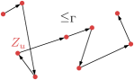
Figure 11: (a) A set of points, and all edges with a slope in $\color[rgb]{0.75,0.30,0.15}[-1,1]$. By Claim 4.9, these edges are all (possibly implicitly) present in $\color[rgb]{0.75,0.30,0.15}\Gamma$. (b) A possible ordering $\color[rgb]{0.75,0.30,0.15}\leq_{\Gamma}$ of the points that respects $\color[rgb]{0.75,0.30,0.15}\Gamma$.

Since all edges on $\color[rgb]{0.75,0.30,0.15}\operatorname{UC}(Z_{u})$ have slopes in $\color[rgb]{0.75,0.30,0.15}[-1,1]$, we immediately have the following corollary.

Corollary 4.10.

The ordering $\color[rgb]{0.75,0.30,0.15}\leq_{\Gamma}$ respects the orders of $\color[rgb]{0.75,0.30,0.15}\operatorname{UC}(Z_{u})$ and $\color[rgb]{0.75,0.30,0.15}\operatorname{LC}(Z_{u})$.

For every node $\color[rgb]{0.75,0.30,0.15}u\in T$, let $\color[rgb]{0.75,0.30,0.15}\leq_{u}$ be the order that $\color[rgb]{0.75,0.30,0.15}\leq_{\Gamma}$ induces on the leaf nodes corresponding to $\color[rgb]{0.75,0.30,0.15}Z_{u}$.

Claim 4.11.

All the orderings $\color[rgb]{0.75,0.30,0.15}\leq_{u}$ can be found in total time $\color[rgb]{0.75,0.30,0.15}O(n)$.

Proof.

To find the orderings $\color[rgb]{0.75,0.30,0.15}\leq_{u}$, perform a topological sort on $\color[rgb]{0.75,0.30,0.15}\Gamma$, in linear time [22, Chapter 22.4]. With each node $\color[rgb]{0.75,0.30,0.15}u$ of $\color[rgb]{0.75,0.30,0.15}T$ store a list $\color[rgb]{0.75,0.30,0.15}L_{u}$, initially empty. We scan the nodes of $\color[rgb]{0.75,0.30,0.15}\Gamma$ in order. Whenever we see a leaf for a point $\color[rgb]{0.75,0.30,0.15}p\in P$, we append $\color[rgb]{0.75,0.30,0.15}p$ to the at most $\color[rgb]{0.75,0.30,0.15}2k$ lists $\color[rgb]{0.75,0.30,0.15}L_{u}$ for the nodes $\color[rgb]{0.75,0.30,0.15}u$ with $\color[rgb]{0.75,0.30,0.15}p\in Z_{u}$. The total running time is $\color[rgb]{0.75,0.30,0.15}O(n+\sum_{u\in T}|Z_{u}|)=O(n)$, and $\color[rgb]{0.75,0.30,0.15}L_{u}$ is sorted according to $\color[rgb]{0.75,0.30,0.15}\leq_{u}$ for each $\color[rgb]{0.75,0.30,0.15}u\in T$. ∎

Claim 4.12.

For any node $\color[rgb]{0.75,0.30,0.15}u\in T$, if $\color[rgb]{0.75,0.30,0.15}Z_{u}$ is sorted according to $\color[rgb]{0.75,0.30,0.15}\leq_{u}$, we can find $\color[rgb]{0.75,0.30,0.15}\operatorname{UC}(Z_{u})$ and $\color[rgb]{0.75,0.30,0.15}\operatorname{LC}(Z_{u})$ in time $\color[rgb]{0.75,0.30,0.15}O(|Z_{u}|)$.

Proof.

We can find $\color[rgb]{0.75,0.30,0.15}\operatorname{UC}(Z_{u})$ by a Graham-type pass through $\color[rgb]{0.75,0.30,0.15}L_{u}$. An example of such a list is shown in Figure 11. That is, we scan $\color[rgb]{0.75,0.30,0.15}L_{u}$ from left to right, maintaining a tentative upper chain $\color[rgb]{0.75,0.30,0.15}U$, stored as a stack. Let $\color[rgb]{0.75,0.30,0.15}r$ be the rightmost point of $\color[rgb]{0.75,0.30,0.15}U$. On scanning a new point $\color[rgb]{0.75,0.30,0.15}p$, we distinguish cases depending in which of the four quadrants $\color[rgb]{0.75,0.30,0.15}\mathcal{C}_{\leftarrow}(r)$, $\color[rgb]{0.75,0.30,0.15}\mathcal{C}_{\uparrow}(r)$, $\color[rgb]{0.75,0.30,0.15}\mathcal{C}_{\rightarrow}(r)$, or $\color[rgb]{0.75,0.30,0.15}\mathcal{C}_{\downarrow}(r)$ it lies in. By Claim 4.1, we know that $\color[rgb]{0.75,0.30,0.15}p\notin\mathcal{C}_{\leftarrow}(r)$. If $\color[rgb]{0.75,0.30,0.15}p\in\mathcal{C}_{\downarrow}(r)$, we discard $\color[rgb]{0.75,0.30,0.15}p$ and continue to the next point in $\color[rgb]{0.75,0.30,0.15}L_{u}$. If $\color[rgb]{0.75,0.30,0.15}p\in\mathcal{C}_{\uparrow}(r)$, we pop $\color[rgb]{0.75,0.30,0.15}r$ from $\color[rgb]{0.75,0.30,0.15}U$ and reassess $\color[rgb]{0.75,0.30,0.15}p$ from the point of view of the new rightmost point of $\color[rgb]{0.75,0.30,0.15}U$. If $\color[rgb]{0.75,0.30,0.15}p\in\mathcal{C}_{\rightarrow}(r)$, we push $\color[rgb]{0.75,0.30,0.15}p$ onto $\color[rgb]{0.75,0.30,0.15}U$.

The algorithm takes $\color[rgb]{0.75,0.30,0.15}O(|Z_{u}|)$ time, because every point is pushed or popped from the stack at most once and because it takes constant time to decide which point to push or pop. Now we argue correctness. For this, we use induction in order to prove that after $\color[rgb]{0.75,0.30,0.15}i$ steps, we have correctly computed the upper chain for the first $\color[rgb]{0.75,0.30,0.15}i$ points in $\color[rgb]{0.75,0.30,0.15}L_{u}$, $\color[rgb]{0.75,0.30,0.15}\operatorname{UC}(L_{i})$. This clearly holds for the first point. Now consider the cases for the $\color[rgb]{0.75,0.30,0.15}(i+1)$-th point $\color[rgb]{0.75,0.30,0.15}p$.

• If $\color[rgb]{0.75,0.30,0.15}p\in\mathcal{C}_{\downarrow}(r)$, then $\color[rgb]{0.75,0.30,0.15}p$ is certainly not on the upper chain. Furthermore, $\color[rgb]{0.75,0.30,0.15}\mathcal{C}_{\downarrow}(p)\subseteq\mathcal{C}_{\downarrow}(r)$, so $\color[rgb]{0.75,0.30,0.15}p$ cannot conflict with any other point on $\color[rgb]{0.75,0.30,0.15}\operatorname{UC}(L_{i})$, so in this case $\color[rgb]{0.75,0.30,0.15}\operatorname{UC}(L_{i+1})=\operatorname{UC}(L_{i})$.

• If $\color[rgb]{0.75,0.30,0.15}p\in\mathcal{C}_{\uparrow}(r)$, then $\color[rgb]{0.75,0.30,0.15}\mathcal{C}_{\uparrow}(p)\subseteq\mathcal{C}_{\uparrow}(r)$ and $\color[rgb]{0.75,0.30,0.15}p$ must be on $\color[rgb]{0.75,0.30,0.15}\operatorname{UC}(L_{i+1})$. Furthermore, every point that we remove from $\color[rgb]{0.75,0.30,0.15}\operatorname{UC}(L_{i})$ has $\color[rgb]{0.75,0.30,0.15}p$ in its upper cone and cannot be on $\color[rgb]{0.75,0.30,0.15}\operatorname{UC}(L_{i+1})$. Now let $\color[rgb]{0.75,0.30,0.15}r^{\prime}$ be the first point of $\color[rgb]{0.75,0.30,0.15}\operatorname{UC}(L_{i})$ that is not popped. Since $\color[rgb]{0.75,0.30,0.15}\mathcal{C}_{\leftarrow}(r^{\prime})\subseteq\mathcal{C}_{\leftarrow}(p)$ and since the remainder of $\color[rgb]{0.75,0.30,0.15}\operatorname{UC}(L_{i})$ lies inside of $\color[rgb]{0.75,0.30,0.15}\mathcal{C}_{\leftarrow}(r^{\prime})$, there are no conflicts between $\color[rgb]{0.75,0.30,0.15}p$ and the points we have not popped. Thus $\color[rgb]{0.75,0.30,0.15}\operatorname{UC}(L_{i+1})$ is computed correctly.

• If $\color[rgb]{0.75,0.30,0.15}p\in\mathcal{C}_{\rightarrow}(r)$, then $\color[rgb]{0.75,0.30,0.15}\mathcal{C}_{\uparrow}(p)\subseteq\mathcal{C}_{\uparrow}(r)\cup\mathcal{C}_{\rightarrow}(r)$, and $\color[rgb]{0.75,0.30,0.15}p$ is on $\color[rgb]{0.75,0.30,0.15}\operatorname{UC}(L_{i+1})$, because $\color[rgb]{0.75,0.30,0.15}\mathcal{C}_{\rightarrow}(r)$ contains no points from $\color[rgb]{0.75,0.30,0.15}L_{i}$. Futhermore, $\color[rgb]{0.75,0.30,0.15}\operatorname{UC}(L_{i})$ is contained in $\color[rgb]{0.75,0.30,0.15}\mathcal{C}_{\leftarrow}(p)$, so $\color[rgb]{0.75,0.30,0.15}p$ conflicts with no point on $\color[rgb]{0.75,0.30,0.15}\operatorname{UC}(L_{i})$ and the result is correct.

This finished the inductive step and the correctness proof. The lower chain is computed in an analogous manner. ∎

Claim 4.13.

For any node $\color[rgb]{0.75,0.30,0.15}u\in T$ and any pair $\color[rgb]{0.75,0.30,0.15}\{u,v\}$ in $\color[rgb]{0.75,0.30,0.15}\mathcal{P}_{u}$, given $\color[rgb]{0.75,0.30,0.15}\operatorname{UC}(Z_{u})$ and $\color[rgb]{0.75,0.30,0.15}\operatorname{LC}(Z_{v})$, we can find the closest pair in $\color[rgb]{0.75,0.30,0.15}Z_{u}\otimes Z_{v}$ in time $\color[rgb]{0.75,0.30,0.15}O(|Z_{u}|+|Z_{v}|)$.

Proof.

Connect the endpoints of $\color[rgb]{0.75,0.30,0.15}\operatorname{UC}(Z_{u})$ and $\color[rgb]{0.75,0.30,0.15}\operatorname{LC}(Z_{v})$ to obtain a simple polygon (note that the two new edges cannot intersect the chains, because $\color[rgb]{0.75,0.30,0.15}\{u,v\}$ has direction $\color[rgb]{0.75,0.30,0.15}\phi=\pi/2$, so by Observation 4.2 $\color[rgb]{0.75,0.30,0.15}\Phi_{uv}\subseteq[\pi/2-8\frac{1}{2}\varepsilon,\pi/2+8\frac{1}{2}\varepsilon]$ and all edges of the chains have slopes in $\color[rgb]{0.75,0.30,0.15}[-1,1]$). Then use the algorithm of Chin and Wang [20] to find the constrained DT of the polygon in time $\color[rgb]{0.75,0.30,0.15}O(|Z_{u}|+|Z_{v}|)$. The closest pair will appear as an edge in this DT, and hence can be found in the claimed time. ∎

Lemma 4.14.

In total linear time, we can find for every $\color[rgb]{0.75,0.30,0.15}u\in T$ and for every pair $\color[rgb]{0.75,0.30,0.15}\{u,v\}\in\mathcal{P}_{u}$ the closest pair in $\color[rgb]{0.75,0.30,0.15}Z_{u}\otimes Z_{v}$.

Proof.

By Claims 4.11, 4.12, 4.13, the time to find all the closest pairs is proportional to

$$\color[rgb]{0.75,0.30,0.15}O(n+\sum_{u\in T}\sum_{\{u,v\}\in\mathcal{P}_{u}}(|Z_{u}|+|Z_{v}|))=O(n+\sum_{u\in T}|Z_{u}|)=O(n),$$

because every $\color[rgb]{0.75,0.30,0.15}v$ appears in only a constant number of $\color[rgb]{0.75,0.30,0.15}\mathcal{P}_{u}$’s. ∎

Putting it together.

We thus obtain the main result of this section.

Theorem 4.15.

Given a compressed quadtree $\color[rgb]{0.75,0.30,0.15}T$ for $\color[rgb]{0.75,0.30,0.15}P$ and $\color[rgb]{0.75,0.30,0.15}\operatorname{\texttt{wspd}}(T)$, we can find a graph $\color[rgb]{0.75,0.30,0.15}H$ with $\color[rgb]{0.75,0.30,0.15}O(n)$ edges such that $\color[rgb]{0.75,0.30,0.15}H$ contains all edges of $\color[rgb]{0.75,0.30,0.15}\operatorname{emst}(P)$. It takes $\color[rgb]{0.75,0.30,0.15}O(n)$ time to construct $\color[rgb]{0.75,0.30,0.15}H$.

Proof.

The fact that $\color[rgb]{0.75,0.30,0.15}H$ contains the EMST follows from Lemmas 4.4, 4.5 and 4.6. The running time follows from the discussion at the beginning of Steps 1 and 2 and from Lemma 4.14. ∎

4.2 Extracting the EMST

We want to extract $\color[rgb]{0.75,0.30,0.15}\operatorname{emst}(P)$, but no general-purpose deterministic linear time pointer machine algorithm for this problem is known: the fastest such algorithm whose running time can be analyzed needs $\color[rgb]{0.75,0.30,0.15}O(n\alpha(n))$ steps [17]. However, the special structure of the graph $\color[rgb]{0.75,0.30,0.15}H$ and the $\color[rgb]{0.75,0.30,0.15}c$-cluster quadtree $\color[rgb]{0.75,0.30,0.15}T$ make it possible to achieve linear time.

We know that $\color[rgb]{0.75,0.30,0.15}H$ contains all EMST edges. Furthermore, by construction each edge of $\color[rgb]{0.75,0.30,0.15}H$ corresponds to a wspd-pair. Thus, we can associate each edge $\color[rgb]{0.75,0.30,0.15}e$ of $\color[rgb]{0.75,0.30,0.15}H$ with two nodes $\color[rgb]{0.75,0.30,0.15}u$ and $\color[rgb]{0.75,0.30,0.15}v$ such that $\color[rgb]{0.75,0.30,0.15}\{u,v\}$ is the wspd-pair for the endpoints of $\color[rgb]{0.75,0.30,0.15}e$. The pruning operation in Step 2 of Section 4.1 ensures that each node is associated with $\color[rgb]{0.75,0.30,0.15}O(1)$ edges of $\color[rgb]{0.75,0.30,0.15}H$, and we store a list of these edges at each node of $\color[rgb]{0.75,0.30,0.15}T$. Now we use Theorem 3.12 to convert our quadtree into a $\color[rgb]{0.75,0.30,0.15}c$-cluster quadtree $\color[rgb]{0.75,0.30,0.15}T$. During this conversion, we can preserve the information about which edges of $\color[rgb]{0.75,0.30,0.15}H$ are associated with which nodes of $\color[rgb]{0.75,0.30,0.15}T$, because each old square overlaps with only a constant number of new squares of similar size. A special case are those edges that have an endpoint associated with a compressed child. During the conversion of Theorem 3.12, compressed children either become regular squares (during the balancing operation), or they correspond to $\color[rgb]{0.75,0.30,0.15}c$-clusters and are replaced by representative points in the parent tree. In the former case, we handle the compressed child just like any regular square, in the latter case, we associate $\color[rgb]{0.75,0.30,0.15}e$ with the square that contains the representative point for the $\color[rgb]{0.75,0.30,0.15}c$-cluster.

Next, we would like ensure for each edge $\color[rgb]{0.75,0.30,0.15}e$ of $\color[rgb]{0.75,0.30,0.15}H$ that the associated squares in $\color[rgb]{0.75,0.30,0.15}T$ have size between $\color[rgb]{0.75,0.30,0.15}\varepsilon|e|/2$ and $\color[rgb]{0.75,0.30,0.15}2\varepsilon|e|$, where $\color[rgb]{0.75,0.30,0.15}|e|$ denotes the length of $\color[rgb]{0.75,0.30,0.15}e$. For the endpoints that were associated with regular squares in the original quadtree, such a square can be found by considering a constant number of ancestors and descendants in $\color[rgb]{0.75,0.30,0.15}T$, by Claim 2.4. If the associated square was a compressed child that has become a regular square, we may need to consider more than a constant number of ancestors, but each such ancestor is considered only a constant number of times, since the compressed child has a constant number of associated edges. If $\color[rgb]{0.75,0.30,0.15}e$ has an endpoint that is now associated with a representative point, we may need to subdivide the square containing the representative point, but by Corollary 3.6 the total work is linear. Thus, in total linear time we can obtain a $\color[rgb]{0.75,0.30,0.15}c$-cluster tree $\color[rgb]{0.75,0.30,0.15}T$ such that each square of $\color[rgb]{0.75,0.30,0.15}T$ is associated with $\color[rgb]{0.75,0.30,0.15}O(1)$ edges of $\color[rgb]{0.75,0.30,0.15}H$ and such that the two associated square of each edge $\color[rgb]{0.75,0.30,0.15}e$ of $\color[rgb]{0.75,0.30,0.15}H$ contain the endpoints of $\color[rgb]{0.75,0.30,0.15}e$ and have size $\color[rgb]{0.75,0.30,0.15}\Theta(\varepsilon|e|)$.

By the cut property of minimum spanning trees, $\color[rgb]{0.75,0.30,0.15}\operatorname{emst}(P)$ is connected within each $\color[rgb]{0.75,0.30,0.15}c$-cluster. Thus, we can process the clusters bottom-up, and we only need to find the EMST within a $\color[rgb]{0.75,0.30,0.15}c$-cluster given that the points in each child are already connected. Within this cluster, $\color[rgb]{0.75,0.30,0.15}T$ is a regular uncompressed quadtree, and we can use the structure of $\color[rgb]{0.75,0.30,0.15}T$ to perform an appropriate variant of Borůvka’s MST algorithm [7, 48] in linear time.

Lemma 4.16.

Let $\color[rgb]{0.75,0.30,0.15}T^{\prime}$ be a subtree of $\color[rgb]{0.75,0.30,0.15}T$ corresponding to a $\color[rgb]{0.75,0.30,0.15}c$-cluster, and let $\color[rgb]{0.75,0.30,0.15}E$ be the edges in $\color[rgb]{0.75,0.30,0.15}H$ associated with $\color[rgb]{0.75,0.30,0.15}T^{\prime}$. Then $\color[rgb]{0.75,0.30,0.15}\operatorname{emst}(P)\cap E$ can be computed in time $\color[rgb]{0.75,0.30,0.15}O(|E|+|V(T^{\prime})|)$.

Proof.

Let $\color[rgb]{0.75,0.30,0.15}\ell$ be the size of the root square of $\color[rgb]{0.75,0.30,0.15}T^{\prime}$. Through a level order traversal of $\color[rgb]{0.75,0.30,0.15}T^{\prime}$ we group the squares in $\color[rgb]{0.75,0.30,0.15}V(T^{\prime})$ by height into layers $\color[rgb]{0.75,0.30,0.15}V_{1}$, $\color[rgb]{0.75,0.30,0.15}V_{2}$, $\color[rgb]{0.75,0.30,0.15}\ldots$, $\color[rgb]{0.75,0.30,0.15}V_{h}$ (where $\color[rgb]{0.75,0.30,0.15}V_{1}$ is the bottommost layer, and $\color[rgb]{0.75,0.30,0.15}V_{h}$ contains only the root). The squares in $\color[rgb]{0.75,0.30,0.15}V_{i}$ have size $\color[rgb]{0.75,0.30,0.15}\ell/2^{h-i}$. As stated above, each square $\color[rgb]{0.75,0.30,0.15}S$ has a constant number of associated edges in $\color[rgb]{0.75,0.30,0.15}E$ that have one endpoint in $\color[rgb]{0.75,0.30,0.15}S$ and length length between $\color[rgb]{0.75,0.30,0.15}|S|/2\varepsilon$ and $\color[rgb]{0.75,0.30,0.15}2|S|/\varepsilon$. To find the EMST, we subdivide the edges into sets $\color[rgb]{0.75,0.30,0.15}E_{i}$, where $\color[rgb]{0.75,0.30,0.15}E_{i}$ contains all edges with length in $\color[rgb]{0.75,0.30,0.15}[\ell/(\varepsilon 2^{h-i}),\ell/(\varepsilon 2^{h-i-1}))$. Given the $\color[rgb]{0.75,0.30,0.15}V_{i}$, we can determine the sets $\color[rgb]{0.75,0.30,0.15}E_{i}$ in total time $\color[rgb]{0.75,0.30,0.15}O(|E|+|V(T^{\prime})|)$, as the edges for $\color[rgb]{0.75,0.30,0.15}E_{i}$ are associated only with squares in $\color[rgb]{0.75,0.30,0.15}V_{i-\alpha}$, $\color[rgb]{0.75,0.30,0.15}V_{i-\alpha+1}$, $\color[rgb]{0.75,0.30,0.15}\ldots$, $\color[rgb]{0.75,0.30,0.15}V_{i+\alpha}$, for some constant $\color[rgb]{0.75,0.30,0.15}\alpha$. Note that every edge in $\color[rgb]{0.75,0.30,0.15}E_{i}$ is crossed by $\color[rgb]{0.75,0.30,0.15}O(1)$ other edges in $\color[rgb]{0.75,0.30,0.15}E_{i}$, because all $\color[rgb]{0.75,0.30,0.15}e\in E_{i}$ have roughly the same length and because every pair of squares in $\color[rgb]{0.75,0.30,0.15}V_{i}$ has only a constant number of associated edges in $\color[rgb]{0.75,0.30,0.15}E_{i}$.

Now we compute the EMST by processing the sets $\color[rgb]{0.75,0.30,0.15}E_{1}$, $\color[rgb]{0.75,0.30,0.15}\ldots$, $\color[rgb]{0.75,0.30,0.15}E_{h}$ in order. Here is how to process $\color[rgb]{0.75,0.30,0.15}E_{i}$. We consider the squares in $\color[rgb]{0.75,0.30,0.15}V_{i}$. Assume that we know for each square of $\color[rgb]{0.75,0.30,0.15}V_{i}$ the connected component in the current partial EMST it meets (initially each $\color[rgb]{0.75,0.30,0.15}c$-cluster is its own component). By the cut property, every square $\color[rgb]{0.75,0.30,0.15}S$ meets only one connected component, as $\color[rgb]{0.75,0.30,0.15}S$ is much smaller than the edges in $\color[rgb]{0.75,0.30,0.15}E_{i}$. Eliminate all edges in $\color[rgb]{0.75,0.30,0.15}E_{i}$ between squares in the same component, and remove duplicate edges between each two components, keeping only the shortest of these edges (this takes $\color[rgb]{0.75,0.30,0.15}O(|E_{i}|)$ time with appropriate pointer manipulation). Then find the shortest edge out of each component and add these edges to the partial EMST. Determine the new components and merge their associated edge sets. This sequence of steps is called a Borůvka-phase. Perform Borůvka-phases until $\color[rgb]{0.75,0.30,0.15}E_{i}$ has no edges left.

By the crossing-number inequality [41, Theorem 4.3.1], the number of edges considered in each phase is proportional to the number $\color[rgb]{0.75,0.30,0.15}r$ of components with an outgoing edge in that phase. Indeed, viewing each component as a supervertex, we have an embedding of a graph with $\color[rgb]{0.75,0.30,0.15}r$ vertices and $\color[rgb]{0.75,0.30,0.15}z$ edges such that there are $\color[rgb]{0.75,0.30,0.15}O(z)$ crossings (since every edge $\color[rgb]{0.75,0.30,0.15}e\in E_{i}$ is crossed by $\color[rgb]{0.75,0.30,0.15}O(1)$ other edges in $\color[rgb]{0.75,0.30,0.15}E_{i}$). Thus, the crossing number inequality yields $\color[rgb]{0.75,0.30,0.15}z^{3}/r^{2}\leq\beta z$, for some constant $\color[rgb]{0.75,0.30,0.15}\beta>0$, so $\color[rgb]{0.75,0.30,0.15}z=O(r)$. Since the number of components at least halves in each phase, and since initially there are at most $\color[rgb]{0.75,0.30,0.15}|V_{i}|$ components, the total time for $\color[rgb]{0.75,0.30,0.15}E_{i}$ is $\color[rgb]{0.75,0.30,0.15}O(|E_{i}|+|V_{i}|)$. Finally, label each square in $\color[rgb]{0.75,0.30,0.15}V_{i+1}$ with the component it meets and proceed with round $\color[rgb]{0.75,0.30,0.15}i+1$. In total, processing $\color[rgb]{0.75,0.30,0.15}T$ takes time $\color[rgb]{0.75,0.30,0.15}O(|V(T^{\prime})|+|E|)$, as desired. ∎

4.3 Finishing Up

We conclude:

Theorem 4.17.

Let $\color[rgb]{0.75,0.30,0.15}P$ be a planar point set and $\color[rgb]{0.75,0.30,0.15}T$ be a compressed quadtree or a $\color[rgb]{0.75,0.30,0.15}c$-cluster quadtree for $\color[rgb]{0.75,0.30,0.15}P$. Then $\color[rgb]{0.75,0.30,0.15}\operatorname{DT}(P)$ can be computed in time $\color[rgb]{0.75,0.30,0.15}O(|P|)$.

Proof.

If $\color[rgb]{0.75,0.30,0.15}T$ is a $\color[rgb]{0.75,0.30,0.15}c$-cluster quadtree, invoke Theorem 3.12 to convert it to a compressed quadtree. Then use Theorem 2.1 to obtain $\color[rgb]{0.75,0.30,0.15}\operatorname{\texttt{wspd}}(T)$. Next, apply Theorem 4.15 to compute the supergraph $\color[rgb]{0.75,0.30,0.15}H$ of $\color[rgb]{0.75,0.30,0.15}\operatorname{emst}(P)$. After that, if necessary, convert $\color[rgb]{0.75,0.30,0.15}T$ to a $\color[rgb]{0.75,0.30,0.15}c$-cluster quadtree for $\color[rgb]{0.75,0.30,0.15}P$ via Theorem 3.12, and apply Lemma 4.16 to each $\color[rgb]{0.75,0.30,0.15}c$-cluster, in a bottom-up manner, to extract $\color[rgb]{0.75,0.30,0.15}\operatorname{emst}(P)$. Finally, apply the algorithm by Chin and Wang [20] to find $\color[rgb]{0.75,0.30,0.15}\operatorname{DT}(P)$. All this takes time $\color[rgb]{0.75,0.30,0.15}O(|P|)$, as claimed. ∎

5 From Delaunay Triangulations to $\color[rgb]{0.75,0.30,0.15}c$-Cluster Quadtrees

For the second direction of our equivalence we need to show how to compute a $\color[rgb]{0.75,0.30,0.15}c$-cluster quadtree for $\color[rgb]{0.75,0.30,0.15}P$ when given $\color[rgb]{0.75,0.30,0.15}\operatorname{DT}(P)$. This was already done by Krznaric and Levcopolous [37, 38], but their algorithm works in a stronger model of computation which includes the floor function and allows access to data at the bit level. As argued in the introduction, we prefer the real RAM/pointer machine, so we need to do some work to adapt their algorithm to our computational model. In this section we describe how Krznaric and Levcopolous’s algorithm can be modified to avoid bucketing and bit-twiddling techniques. The only difference is that in the resulting $\color[rgb]{0.75,0.30,0.15}c$-cluster quadtree the squares for the $\color[rgb]{0.75,0.30,0.15}c$-clusters are not perfectly aligned with the squares of the parent quadtree. In our setting, this does not matter. The goal of this section is to prove the following theorem.

Theorem 5.1.

Given $\color[rgb]{0.75,0.30,0.15}\operatorname{DT}(P)$, we can compute a $\color[rgb]{0.75,0.30,0.15}c$-cluster quadtree for $\color[rgb]{0.75,0.30,0.15}P$ in linear deterministic time on a pointer machine.

In the following, we will refer to the paper by Krznaric and Levcopolous [38] as KL. Our description is meant to be self-contained; however, we refer the reader to KL for more intuition and a more elaborate description of the main ideas.

5.1 Terminology

We begin by recalling some terminology from KL.

• neighborhood. The neighborhood of a square $\color[rgb]{0.75,0.30,0.15}S$ of a quadtree consists of the 25 squares of size $\color[rgb]{0.75,0.30,0.15}|S|$ concentric around $\color[rgb]{0.75,0.30,0.15}S$ (including $\color[rgb]{0.75,0.30,0.15}S$); see Figure 12.

• direct neighborhood. The direct neighborhood of a square $\color[rgb]{0.75,0.30,0.15}S$ consists of the 9 squares of size $\color[rgb]{0.75,0.30,0.15}|S|$ directly adjacent to $\color[rgb]{0.75,0.30,0.15}S$ (including $\color[rgb]{0.75,0.30,0.15}S$); see Figure 12.

• star of a square. Let $\color[rgb]{0.75,0.30,0.15}P$ be a planar point set, and let $\color[rgb]{0.75,0.30,0.15}S$ be a square. The star of $\color[rgb]{0.75,0.30,0.15}S$, denoted by $\color[rgb]{0.75,0.30,0.15}\bigstar(S)$, is the set of all edges $\color[rgb]{0.75,0.30,0.15}e$ in $\color[rgb]{0.75,0.30,0.15}\operatorname{DT}(P)$ such that (i) $\color[rgb]{0.75,0.30,0.15}e$ has one endpoint inside $\color[rgb]{0.75,0.30,0.15}S$ and one endpoint outside the neighborhood of $\color[rgb]{0.75,0.30,0.15}S$; and (ii) $\color[rgb]{0.75,0.30,0.15}|e|\leq 16|S|$, where $\color[rgb]{0.75,0.30,0.15}|e|$ is the length of $\color[rgb]{0.75,0.30,0.15}e$.

• dilation. Let $\color[rgb]{0.75,0.30,0.15}P$ be a planar point set, and $\color[rgb]{0.75,0.30,0.15}G$ a connected plane graph with vertex set $\color[rgb]{0.75,0.30,0.15}P$. The dilation of $\color[rgb]{0.75,0.30,0.15}P$ is the distortion between the shortest path metric in $\color[rgb]{0.75,0.30,0.15}G$ and the Euclidean distance, i.e., the maximum ratio, over all pairs of distinct points $\color[rgb]{0.75,0.30,0.15}p,q\in P$, between the length of the shortest path in $\color[rgb]{0.75,0.30,0.15}G$ from $\color[rgb]{0.75,0.30,0.15}p$ to $\color[rgb]{0.75,0.30,0.15}q$, and $\color[rgb]{0.75,0.30,0.15}|pq|$. There are many families of planar graphs whose dilation is bounded by a constant [23]. In particular, for any planar point set $\color[rgb]{0.75,0.30,0.15}P$, the dilation of $\color[rgb]{0.75,0.30,0.15}\operatorname{DT}(P)$ is bounded by $\color[rgb]{0.75,0.30,0.15}2\pi/(3\cos(\pi/6))\leq 2.42$ [35].

• orientation. The orientation of a line segment $\color[rgb]{0.75,0.30,0.15}e$ is the angle the line through $\color[rgb]{0.75,0.30,0.15}e$ makes with the $\color[rgb]{0.75,0.30,0.15}x$-axis.

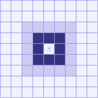
Figure 12: The neighborhood of a square $\color[rgb]{0.75,0.30,0.15}S$. The direct neighbors are shown in dark blue, the others in light blue.

5.2 Preprocessing

By Theorem 3.1, we can obtain a $\color[rgb]{0.75,0.30,0.15}c$-cluster tree $\color[rgb]{0.75,0.30,0.15}T_{c}$ for $\color[rgb]{0.75,0.30,0.15}P$ in linear time, given $\color[rgb]{0.75,0.30,0.15}\operatorname{DT}(P)$. Thus, we only need to construct the regular quadtrees $\color[rgb]{0.75,0.30,0.15}T_{u}^{Q}$ for each node $\color[rgb]{0.75,0.30,0.15}u$ in $\color[rgb]{0.75,0.30,0.15}T_{c}$. This is done by processing each node of $\color[rgb]{0.75,0.30,0.15}T_{c}$ individually. First, however, we need to perform a preprocessing step in order to find for each edge $\color[rgb]{0.75,0.30,0.15}e$ of $\color[rgb]{0.75,0.30,0.15}\operatorname{DT}(P)$ the node of $\color[rgb]{0.75,0.30,0.15}T_{c}$ that is the least common ancestor of $\color[rgb]{0.75,0.30,0.15}e$’s endpoints. For every node $\color[rgb]{0.75,0.30,0.15}u\in T_{c}$, we define $\color[rgb]{0.75,0.30,0.15}\texttt{out}(u)$ as the set of edges in $\color[rgb]{0.75,0.30,0.15}\operatorname{DT}(P)$ that have exactly one endpoint in $\color[rgb]{0.75,0.30,0.15}P_{u}$ and both endpoints in $\color[rgb]{0.75,0.30,0.15}P_{\overline{u}}$. Clearly, every edge is contained in exactly two sets $\color[rgb]{0.75,0.30,0.15}\texttt{out}(u)$ and $\color[rgb]{0.75,0.30,0.15}\texttt{out}(v)$, where $\color[rgb]{0.75,0.30,0.15}u$ and $\color[rgb]{0.75,0.30,0.15}v$ are siblings in $\color[rgb]{0.75,0.30,0.15}T_{c}$. The following is a simple variant of a lemma from KL [38, Lemma 3].

Lemma 5.2 (Krznaric-Levcopolous).

Let $\color[rgb]{0.75,0.30,0.15}P$ be a planar $\color[rgb]{0.75,0.30,0.15}n$-point set. Given $\color[rgb]{0.75,0.30,0.15}DT(P)$ and a $\color[rgb]{0.75,0.30,0.15}c$-cluster tree $\color[rgb]{0.75,0.30,0.15}T_{c}$ for $\color[rgb]{0.75,0.30,0.15}P$, the sets $\color[rgb]{0.75,0.30,0.15}\texttt{out}(u)$ for every node $\color[rgb]{0.75,0.30,0.15}u\in T_{c}$ can be found in overall $\color[rgb]{0.75,0.30,0.15}O(n)$ time and space on a pointer machine.

Proof.

KL show how to reduce the problem of determining the sets $\color[rgb]{0.75,0.30,0.15}\texttt{out}(u)$ to $\color[rgb]{0.75,0.30,0.15}O(n)$ off-line least-common ancestor (lca) queries in two appropriate trees. For the lca-queries, they invoke an algorithm by Harel and Tarjan [34] that requires the word RAM. However, since all lca-queries are known in advance (i.e., the queries are off-line), we may instead use an algorithm by Buchsbaum et al. [10, Theorem 6.1] which requires $\color[rgb]{0.75,0.30,0.15}O(n)$ time and space on a pointer machine. ∎

5.3 Processing a Single Node of $\color[rgb]{0.75,0.30,0.15}T_{c}$

We now describe the preprocessing that is necessary on a single node $\color[rgb]{0.75,0.30,0.15}u$ of $\color[rgb]{0.75,0.30,0.15}T_{c}$ before the quadtree $\color[rgb]{0.75,0.30,0.15}T_{u}^{Q}$ can be constructed. Let $\color[rgb]{0.75,0.30,0.15}v_{1},v_{2},\ldots,v_{m}$ be the children of $\color[rgb]{0.75,0.30,0.15}u$. For each child $\color[rgb]{0.75,0.30,0.15}v_{i}$, let $\color[rgb]{0.75,0.30,0.15}\delta_{i}:=d(P_{v_{i}},P_{u}\setminus P_{v_{i}})$.

Claim 5.3.

For $\color[rgb]{0.75,0.30,0.15}i=1,\ldots,m$, $\color[rgb]{0.75,0.30,0.15}\texttt{out}(v_{i})$ contains an edge of length $\color[rgb]{0.75,0.30,0.15}\delta_{i}$.

Proof.

If $\color[rgb]{0.75,0.30,0.15}\operatorname{DT}(P)$ contains an edge $\color[rgb]{0.75,0.30,0.15}e$ with an endpoint in $\color[rgb]{0.75,0.30,0.15}P_{v_{i}}$ and with length $\color[rgb]{0.75,0.30,0.15}\delta_{i}$, then $\color[rgb]{0.75,0.30,0.15}e$ must be in $\color[rgb]{0.75,0.30,0.15}\texttt{out}(v_{i})$, by the definition of a $\color[rgb]{0.75,0.30,0.15}c$-cluster. Since $\color[rgb]{0.75,0.30,0.15}\operatorname{emst}(P)$ is a subgraph of $\color[rgb]{0.75,0.30,0.15}\operatorname{DT}(P)$, it thus suffices to show that $\color[rgb]{0.75,0.30,0.15}\operatorname{emst}(P)$ contains such an edge. Consider running Kruskal’s MST algorithm on $\color[rgb]{0.75,0.30,0.15}P$. According to the definition of a $\color[rgb]{0.75,0.30,0.15}c$-cluster, by the time the algorithm considers the edge $\color[rgb]{0.75,0.30,0.15}e$ that achieves $\color[rgb]{0.75,0.30,0.15}\delta_{i}$, the partially constructed EMST contains exactly one connected component that has precisely the points in $\color[rgb]{0.75,0.30,0.15}P_{v_{i}}$. Therefore, $\color[rgb]{0.75,0.30,0.15}e\in\operatorname{emst}(P)$, and the claim follows. ∎

Initialization.

By scanning the sets $\color[rgb]{0.75,0.30,0.15}\texttt{out}(v_{i})$, we determine a child $\color[rgb]{0.75,0.30,0.15}v_{j}$ with minimum $\color[rgb]{0.75,0.30,0.15}\delta_{j}$ (by Claim 5.3 a shortest edge in $\color[rgb]{0.75,0.30,0.15}\texttt{out}(v_{i})$ has length $\color[rgb]{0.75,0.30,0.15}\delta_{i}$). We may assume that $\color[rgb]{0.75,0.30,0.15}j=1$. Let $\color[rgb]{0.75,0.30,0.15}S_{1}$ be a square that contains $\color[rgb]{0.75,0.30,0.15}P_{v_{1}}$ and that has side-length $\color[rgb]{0.75,0.30,0.15}\delta_{1}/8$. Let $\color[rgb]{0.75,0.30,0.15}\alpha$ be the smallest integer such that four squares of size $\color[rgb]{0.75,0.30,0.15}2^{\alpha-1}\delta_{1}/8$ cover all of $\color[rgb]{0.75,0.30,0.15}P_{u}$. Lemma 3.4 implies that $\color[rgb]{0.75,0.30,0.15}\alpha=O(m)$.

The goal is to compute $\color[rgb]{0.75,0.30,0.15}T_{u}^{Q}$, the balanced regular quadtree aligned at $\color[rgb]{0.75,0.30,0.15}S_{1}$ such that each $\color[rgb]{0.75,0.30,0.15}P_{v_{i}}$ is contained in squares of size $\color[rgb]{0.75,0.30,0.15}\delta_{i}/8$. To begin, we use $\color[rgb]{0.75,0.30,0.15}S_{1}$ to initialize $\color[rgb]{0.75,0.30,0.15}T_{u}^{Q}$ as the partial balanced quadtree $\color[rgb]{0.75,0.30,0.15}T_{u}^{Q}$ shown in Figure 13.

Figure 13: The initial quadtree.

Every square $\color[rgb]{0.75,0.30,0.15}S$ of $\color[rgb]{0.75,0.30,0.15}T_{u}^{Q}$ stores the following fields:

• parent: a pointer to the parent square, nil for the root;

• children: pointers for the four children of $\color[rgb]{0.75,0.30,0.15}S$, nil for a leaf;

• neighbors: links to the four orthogonal neighbors of $\color[rgb]{0.75,0.30,0.15}S$ in the quadtree $\color[rgb]{0.75,0.30,0.15}T_{u}^{Q}$ with size $\color[rgb]{0.75,0.30,0.15}|S|$ (or size $\color[rgb]{0.75,0.30,0.15}2|S|$, if no smaller neighbor exists);

The fields parent, children, and neighbors are initialized for all the nodes in $\color[rgb]{0.75,0.30,0.15}T_{Q}$.

Lemma 5.4.

The total time for the initialization phase is $\color[rgb]{0.75,0.30,0.15}O(m+\sum_{i=1}^{m}|\texttt{out}(v_{i})|)$.

Proof.

By Lemma 3.4, the initial size of $\color[rgb]{0.75,0.30,0.15}T_{u}^{Q}$ is $\color[rgb]{0.75,0.30,0.15}O(m)$. All other operations consist of scanning the out-lists or are linear in the size of $\color[rgb]{0.75,0.30,0.15}T_{u}^{Q}$. ∎

5.4 Building the Tree $\color[rgb]{0.75,0.30,0.15}T_{u}^{Q}$

$\color[rgb]{0.75,0.30,0.15}\texttt{explore}(\mathcal{S},\texttt{maxsize})$

1. Set $\color[rgb]{0.75,0.30,0.15}\texttt{active}:=\mathcal{S}$.

2. Set $\color[rgb]{0.75,0.30,0.15}\texttt{newActive}:=\emptyset$.

3. Until the squares in active have size greater than maxsize:

   1. For every square $\color[rgb]{0.75,0.30,0.15}S$ in active call the function $\color[rgb]{0.75,0.30,0.15}\texttt{findStar}(S)$ to determine $\color[rgb]{0.75,0.30,0.15}\bigstar(S)$. Append $\color[rgb]{0.75,0.30,0.15}\overline{S}$ to newActive, if it is not present yet.

   2. For every edge $\color[rgb]{0.75,0.30,0.15}e\in\bigcup_{S\in\texttt{active}}\bigstar(S)$, if $\color[rgb]{0.75,0.30,0.15}e$ has an endpoint in an undiscovered cluster, call the function $\color[rgb]{0.75,0.30,0.15}\texttt{newCluster}(S,e)$, and append all the squares returned by this call to newActive.

   3. Set $\color[rgb]{0.75,0.30,0.15}\texttt{active}:=\texttt{newActive}$.

$\color[rgb]{0.75,0.30,0.15}\texttt{newCluster}(S,e)$

1. Walk along $\color[rgb]{0.75,0.30,0.15}e$ through the current $\color[rgb]{0.75,0.30,0.15}T_{u}^{Q}$ to find the square $\color[rgb]{0.75,0.30,0.15}S^{\prime}$ of $\color[rgb]{0.75,0.30,0.15}T_{u}^{Q}$ that contains the other endpoint of $\color[rgb]{0.75,0.30,0.15}e$. This tracing is done by following the appropriate neighbor pointers from $\color[rgb]{0.75,0.30,0.15}S$.

2. Refine $\color[rgb]{0.75,0.30,0.15}T_{u}^{Q}$ for the new cluster, and let $\color[rgb]{0.75,0.30,0.15}\mathcal{S}^{\prime}$ be the set of leaf squares containing the newly discovered cluster.

3. Call $\color[rgb]{0.75,0.30,0.15}\texttt{explore}(\mathcal{S}^{\prime},\text{size of squares in {active}})$. Afterwards, return the active squares from the recursive call.

Algorithm 2 Computing a $\color[rgb]{0.75,0.30,0.15}c$-cluster quadtree for the children of a $\color[rgb]{0.75,0.30,0.15}c$-cluster.

Now we build the tree $\color[rgb]{0.75,0.30,0.15}T_{u}^{Q}$ by a traversing $\color[rgb]{0.75,0.30,0.15}\operatorname{DT}(P)$ in a way reminiscent of Dijkstra’s algorithm [22]. In their algorithm, KL make extensive use of the floor function in order to locate points inside their quadtree squares. The purpose of this section is to argue that this point location work can be done through local traversal of the quadtree, without the floor function. Refer to Algorithm 2. The heart of the algorithm is the procedure explore, which is initially called as $\color[rgb]{0.75,0.30,0.15}\texttt{explore}(\{S_{1}\},2^{\alpha-1}\delta_{1}/8)$. The procedure explore builds the tree $\color[rgb]{0.75,0.30,0.15}T_{u}^{Q}$ level by level, beginning with the level of $\color[rgb]{0.75,0.30,0.15}S_{1}$. At each point, it maintains a set active of all squares at the current level that contain a cluster that has already been processed. For each such square $\color[rgb]{0.75,0.30,0.15}S$, it calls a function findStar. This function returns all edges of the Delaunay triangulation that have one endpoint in $\color[rgb]{0.75,0.30,0.15}S$ and have length $\color[rgb]{0.75,0.30,0.15}\alpha|S|$, for a constant $\color[rgb]{0.75,0.30,0.15}\alpha$. Using findStar we can new clusters whose distance from the active clusters is comparable to the size of the squares in the current level. We will say more about the implementation findStar below. For each new cluster, we call the procedure newCluster which adds more squares to $\color[rgb]{0.75,0.30,0.15}T_{u}^{Q}$ to accommodate the new cluster and recursively explores the short edges out of this new cluster. After the recursive call has finished, we can continue the exploration of the tree at the current level.

We now give the details for the refinement in Step 2 of newCluster: Let $\color[rgb]{0.75,0.30,0.15}v_{j}$ be the cluster that contains the other endpoint $\color[rgb]{0.75,0.30,0.15}q$ of $\color[rgb]{0.75,0.30,0.15}e$ (we can find $\color[rgb]{0.75,0.30,0.15}v_{j}$ in constant time, since $\color[rgb]{0.75,0.30,0.15}e\in\texttt{out}(v_{j})$, and since for each edge we store the two clusters whose out-lists contain it). Subdivide the current leaf square containing $\color[rgb]{0.75,0.30,0.15}q$ (and possibly also its neighbors if they contain points from $\color[rgb]{0.75,0.30,0.15}P_{v_{j}}$) in quadtree-fashion until $\color[rgb]{0.75,0.30,0.15}P_{v_{j}}$ is contained in squares of size $\color[rgb]{0.75,0.30,0.15}\delta_{j}/8$. Then balance the quadtree and update the neighbor pointers accordingly.

The algorithm is recursive, and at each point there exists a sequence $\color[rgb]{0.75,0.30,0.15}\mathcal{E}_{1}$, $\color[rgb]{0.75,0.30,0.15}\mathcal{E}_{2}$, $\color[rgb]{0.75,0.30,0.15}\ldots$, $\color[rgb]{0.75,0.30,0.15}\mathcal{E}_{z}$ of instantiations (i.e., stack frames) of explore, where $\color[rgb]{0.75,0.30,0.15}\mathcal{E}_{i+1}$ was invoked by $\color[rgb]{0.75,0.30,0.15}\mathcal{E}_{i}$. Each $\color[rgb]{0.75,0.30,0.15}\mathcal{E}_{i}$ has a set $\color[rgb]{0.75,0.30,0.15}\texttt{active}_{i}$ of active squares, such that all squares in each $\color[rgb]{0.75,0.30,0.15}\texttt{active}_{i}$ have the same size, and such that the squares in $\color[rgb]{0.75,0.30,0.15}\texttt{active}_{i+1}$ are not larger than the squares in $\color[rgb]{0.75,0.30,0.15}\texttt{active}_{i}$. We say that a square is active if it is contained in $\color[rgb]{0.75,0.30,0.15}\texttt{active}^{T}:=\bigcup_{i}\texttt{active}_{i}$. The neighborhood of $\color[rgb]{0.75,0.30,0.15}\texttt{active}^{T}$ is the union of the neighborhoods of all boxes in active. We maintain the following invariant:

Invariant 5.5.

At all times during the execution of explore, all undiscovered $\color[rgb]{0.75,0.30,0.15}c$-clusters lie outside the neighborhood of $\color[rgb]{0.75,0.30,0.15}\texttt{active}^{T}$.

Claim 5.6.

Invariant 5.5 is maintained by explore.

Proof.

The set $\color[rgb]{0.75,0.30,0.15}\texttt{active}^{T}$ only changes in Steps 1 and 3c. The invariant is maintained in Step 1, since the size of the squares in $\color[rgb]{0.75,0.30,0.15}\mathcal{S}$ (i.e., $\color[rgb]{0.75,0.30,0.15}\delta_{i}/8)$ is chosen such that their neighborhoods can contain no point from any other cluster.

Let us now consider Step 3c. The set newActive contains two kinds of squares: (i) the parents of squares processed in the current iteration of the main loop; and (ii) squares that were added to newActive after a recursive call. We only need to focus on squares of type (i), since squares of type (ii) are already added to $\color[rgb]{0.75,0.30,0.15}\texttt{active}^{T}$ during the recursive call. Suppose that $\color[rgb]{0.75,0.30,0.15}\texttt{active}^{T}$ contains a square $\color[rgb]{0.75,0.30,0.15}S$ whose neighborhood has a point $\color[rgb]{0.75,0.30,0.15}p\in P$ in an undiscovered cluster. Since $\color[rgb]{0.75,0.30,0.15}S\in\texttt{active}^{T}$, there is a point $\color[rgb]{0.75,0.30,0.15}q\in P\cap\mathcal{S}$, and by the definition of neighborhood, we have $\color[rgb]{0.75,0.30,0.15}d(p,q)\leq 3|S|$. However, since the dilation of $\color[rgb]{0.75,0.30,0.15}\operatorname{DT}(P)$ is at most $\color[rgb]{0.75,0.30,0.15}2.5$ [35], $\color[rgb]{0.75,0.30,0.15}\operatorname{DT}(P)$ contains a path $\color[rgb]{0.75,0.30,0.15}\pi$ of length at most $\color[rgb]{0.75,0.30,0.15}8|S|$ from $\color[rgb]{0.75,0.30,0.15}p$ to $\color[rgb]{0.75,0.30,0.15}q$. Let $\color[rgb]{0.75,0.30,0.15}p^{\prime}$ be the last discovered point along $\color[rgb]{0.75,0.30,0.15}\pi$. The point $\color[rgb]{0.75,0.30,0.15}p^{\prime}$ lies in an active square $\color[rgb]{0.75,0.30,0.15}S^{\prime}$ with $\color[rgb]{0.75,0.30,0.15}|S^{\prime}|\geq|S|$, and the edge $\color[rgb]{0.75,0.30,0.15}e$ leaving $\color[rgb]{0.75,0.30,0.15}p^{\prime}$ on $\color[rgb]{0.75,0.30,0.15}\pi$ has length at most $\color[rgb]{0.75,0.30,0.15}8|S^{\prime}|$. Therefore, $\color[rgb]{0.75,0.30,0.15}e\in\bigstar(S^{\prime\prime})$ for a descendant $\color[rgb]{0.75,0.30,0.15}S^{\prime\prime}$ of $\color[rgb]{0.75,0.30,0.15}S^{\prime}$, which contradicts the fact that $\color[rgb]{0.75,0.30,0.15}p^{\prime}$ is the last discovered point along $\color[rgb]{0.75,0.30,0.15}\pi$. ∎

Lemma 5.7.

The total running time of explore, excluding the calls to findStar, is $\color[rgb]{0.75,0.30,0.15}O(m+\sum_{i=1}^{m}|\texttt{out}(v_{i})|)$.

Proof.

All squares appearing in $\color[rgb]{0.75,0.30,0.15}\texttt{active}^{T}$ are ancestors of non-empty leaf squares in the final tree $\color[rgb]{0.75,0.30,0.15}T_{u}^{Q}$. Therefore, by Lemma 3.4, the total number of iterations for the loop in Step 3a is $\color[rgb]{0.75,0.30,0.15}O(m)$. Furthermore, $\color[rgb]{0.75,0.30,0.15}\bigstar(S)$ contains only edges of length $\color[rgb]{0.75,0.30,0.15}\Theta(|S|)$, so every edge appears in only a constant number of stars. It follows that the total size of the $\color[rgb]{0.75,0.30,0.15}\bigstar$-lists, and hence the total number of iterations of the loop in Step 3b is $\color[rgb]{0.75,0.30,0.15}O(\sum_{i=1}^{m}|\texttt{out}(v_{i})|)$.

It remains to bound the time for tracing the edges and balancing the tree. Since $\color[rgb]{0.75,0.30,0.15}T_{u}^{Q}$ is balanced and since $\color[rgb]{0.75,0.30,0.15}\bigstar(S)$ contains only edges of length $\color[rgb]{0.75,0.30,0.15}\Theta(|S|)$, the tracing along the neighbor pointers of an edge takes constant time (since we traverse a constant number of boxes of size $\color[rgb]{0.75,0.30,0.15}\Theta(|S|)$). By Invariant 5.5, the other endpoint of the edge is contained in a leaf square of the current $\color[rgb]{0.75,0.30,0.15}T_{u}^{Q}$ of size $\color[rgb]{0.75,0.30,0.15}\Theta(|S|)$. (This is because the quadtree is balanced and because the other endpoint of the edge lies outside the neighborhood of the active squares.) Therefore, the time to build the balanced quadtree for the new leaf squares containing the newly discovered cluster can be charged to the corresponding nodes in the final $\color[rgb]{0.75,0.30,0.15}T_{u}^{Q}$, of which there are $\color[rgb]{0.75,0.30,0.15}O(m)$. Furthermore, note that by Invariant 5.5, balancing the quadtree for the newly discovered leaf squares does not affect any descendants of the active squares. ∎

5.5 Implementing findStar

KL show how to exploit the geometric properties of the Delaunay triangulation in order to implement the function findStar, quickly. For this, they store two additional fields with each active square, called characteristic and shortcuts [38, Section 6], and they explain how to maintain these lists throughout the procedure. This part of the algorithm works on a real RAM/pointer machine without any further modification, so we just state their result.

Lemma 5.8.

The total time for all calls to findStar and the maintenance of the required data structures is $\color[rgb]{0.75,0.30,0.15}O(m+\sum_{i=1}^{m}|\texttt{out}(v_{i})|)$. ∎

5.6 Putting Everything Together

We can now finally prove Theorem 5.1.

Proof of Theorem 5.1.

First, we use Theorem 3.1 to find a $\color[rgb]{0.75,0.30,0.15}c$-cluster tree $\color[rgb]{0.75,0.30,0.15}T_{c}$ for $\color[rgb]{0.75,0.30,0.15}P$ in $\color[rgb]{0.75,0.30,0.15}O(n)$ time. Next, we use the algorithm from Section 5.2 to preprocess the tree. By Lemma 5.2, this also takes $\color[rgb]{0.75,0.30,0.15}O(n)$ time. Finally, we process each node of $\color[rgb]{0.75,0.30,0.15}T_{c}$ using the algorithm from Section 5.3. By Lemmas 5.4, 5.7, and 5.8, this takes total time $\color[rgb]{0.75,0.30,0.15}\sum_{j}1+|\texttt{out}(v_{j})|$, where the sum ranges over all the nodes of $\color[rgb]{0.75,0.30,0.15}T_{c}$. This sum is $\color[rgb]{0.75,0.30,0.15}O(n)$ because there are $\color[rgb]{0.75,0.30,0.15}O(n)$ nodes in $\color[rgb]{0.75,0.30,0.15}T_{c}$, and because every edge of $\color[rgb]{0.75,0.30,0.15}\operatorname{DT}(P)$ appears in exactly two out-lists. Hence, the total running time is linear, as claimed. ∎

6 Applications

As mentioned in the introduction, our result yields deterministic versions of several recent randomized algorithms related to DTs. Firstly, we can immediately derandomize an algorithm for hereditary DTs by Chazelle et al. [18, 19]:

Corollary 6.1.

Let $\color[rgb]{0.75,0.30,0.15}P$ a planar $\color[rgb]{0.75,0.30,0.15}n$-point set, and let $\color[rgb]{0.75,0.30,0.15}S\subseteq P$. Given $\color[rgb]{0.75,0.30,0.15}\operatorname{DT}(P)$, we can find $\color[rgb]{0.75,0.30,0.15}\operatorname{DT}(S)$ in deterministic time $\color[rgb]{0.75,0.30,0.15}O(n)$ on a pointer machine.

Proof.

Use Theorem 5.1 to find a $\color[rgb]{0.75,0.30,0.15}c$-cluster quadtree $\color[rgb]{0.75,0.30,0.15}T$ for $\color[rgb]{0.75,0.30,0.15}P$, remove the leaves for $\color[rgb]{0.75,0.30,0.15}P\setminus S$ from $\color[rgb]{0.75,0.30,0.15}T$ and trim it appropriately. Finally, apply Theorem 4.17 to extract $\color[rgb]{0.75,0.30,0.15}\operatorname{DT}(S)$ from $\color[rgb]{0.75,0.30,0.15}T$, in time $\color[rgb]{0.75,0.30,0.15}O(n)$. ∎

Secondly, we obtain deterministic analogues of the algorithms by Buchin et al. [8] to preprocess imprecise point sets for faster DTs. For example, we can prove the following:

Corollary 6.2.

Let $\color[rgb]{0.75,0.30,0.15}\mathcal{R}=\langle R_{1},R_{2},\ldots,R_{n}\rangle$ be a sequence of $\color[rgb]{0.75,0.30,0.15}n$ $\color[rgb]{0.75,0.30,0.15}\beta$-fat planar regions so that no point in $\color[rgb]{0.75,0.30,0.15}\mathbb{R}^{2}$ meets more than $\color[rgb]{0.75,0.30,0.15}k$ of them. We can preprocess $\color[rgb]{0.75,0.30,0.15}\mathcal{R}$ in $\color[rgb]{0.75,0.30,0.15}O(n\log n)$ deterministic time into an $\color[rgb]{0.75,0.30,0.15}O(n)$-size data structure so that given a sequence of $\color[rgb]{0.75,0.30,0.15}n$ points $\color[rgb]{0.75,0.30,0.15}P=\langle p_{1},p_{2},\ldots,p_{n}\rangle$ with $\color[rgb]{0.75,0.30,0.15}p_{i}\in R_{i}$ for all $\color[rgb]{0.75,0.30,0.15}i$, we can find $\color[rgb]{0.75,0.30,0.15}\operatorname{DT}(P)$ in deterministic time $\color[rgb]{0.75,0.30,0.15}O(n\log(k/\beta))$ on a pointer machine.

Proof.

The method of Buchin et al. [8, Theorem 4.3 and Corollary 5.6] proceeds by computing a representative quadtree $\color[rgb]{0.75,0.30,0.15}T$ for $\color[rgb]{0.75,0.30,0.15}\mathcal{R}$. Given $\color[rgb]{0.75,0.30,0.15}P$, the algorithm finds for every point in $\color[rgb]{0.75,0.30,0.15}P$ the leaf square of $\color[rgb]{0.75,0.30,0.15}T$ that contains it, and then uses this information to obtain a compressed quadtree $\color[rgb]{0.75,0.30,0.15}T^{\prime}$ for $\color[rgb]{0.75,0.30,0.15}P$ in time $\color[rgb]{0.75,0.30,0.15}O(n\log(k/\beta))$. However, $\color[rgb]{0.75,0.30,0.15}T^{\prime}$ is skewed in the sense that not all its squares need to be perfectly aligned and that some squares can be cut off. However, the authors argue that even in this case $\color[rgb]{0.75,0.30,0.15}\operatorname{\texttt{wspd}}(T)$ takes $\color[rgb]{0.75,0.30,0.15}O(n)$ time and yields a linear-size WSPD [8, Appendix B]. The main observation [8, Observation B.1] is that any (truncated) square $\color[rgb]{0.75,0.30,0.15}S$ in $\color[rgb]{0.75,0.30,0.15}T^{\prime}$ is adjacent to at least one square whose area is at least a constant fraction of the area $\color[rgb]{0.75,0.30,0.15}S$ would have without clipping. Since in skewed quadtrees the size of a node is at most half the size of its parent, the argument of Lemma 4.4 still applies. To see that Lemma 4.5 holds, we need to check that the volume argument goes through. For this, note that by the main observation of Buchin et al., we can assign every square $\color[rgb]{0.75,0.30,0.15}R_{w}$ (the notation is as in the proof of Lemma 4.5) to an adjacent square of comparable size at distance $\color[rgb]{0.75,0.30,0.15}O(\varepsilon)$ from $\color[rgb]{0.75,0.30,0.15}A$. Since every such square is charged by disjoint descendants from a constant number of neighbors, the volume argument still applies, and Lemma 4.5 holds. Lemma 4.14 only relies on well-separation and the combinatorial structure of $\color[rgb]{0.75,0.30,0.15}T$, and hence remains valid. Finally, in order to apply Lemma 4.16, we need to turn $\color[rgb]{0.75,0.30,0.15}T^{\prime}$ into a $\color[rgb]{0.75,0.30,0.15}c$-cluster quadtree, which takes linear time by Theorem 3.12. Thus, the total running time is $\color[rgb]{0.75,0.30,0.15}O(n\log(k/\beta)$, as claimed. ∎

Finally, Buchin and Mulzer [9] showed that for word RAMs, DTs are no harder than sorting. We can now do it deterministically. Let $\color[rgb]{0.75,0.30,0.15}\texttt{sort}(n)$ be the time to sort $\color[rgb]{0.75,0.30,0.15}n$ integers on a $\color[rgb]{0.75,0.30,0.15}w$-bit word RAM. The best deterministic bound for $\color[rgb]{0.75,0.30,0.15}\texttt{sort}(n)$ is $\color[rgb]{0.75,0.30,0.15}O(n\log\log n)$ [32].

Corollary 6.3.

Let $\color[rgb]{0.75,0.30,0.15}P$ be a planar $\color[rgb]{0.75,0.30,0.15}n$-point set given by $\color[rgb]{0.75,0.30,0.15}w$-bit integers, for some word-size $\color[rgb]{0.75,0.30,0.15}w\geq\log n$. We can find $\color[rgb]{0.75,0.30,0.15}\operatorname{DT}(P)$ in deterministic time $\color[rgb]{0.75,0.30,0.15}O(\emph{{sort}}(n))$ on a word RAM supporting the shuffle-operation.

Proof.

Buchin and Mulzer [9] show how to find a compressed quadtree $\color[rgb]{0.75,0.30,0.15}T$ for $\color[rgb]{0.75,0.30,0.15}P$ in time $\color[rgb]{0.75,0.30,0.15}O(\texttt{sort}(n))$, using the shuffle-operation. They actually do not find the squares of the quadtree, only the combinatorial structure of $\color[rgb]{0.75,0.30,0.15}T$ and the bounding boxes $\color[rgb]{0.75,0.30,0.15}B_{v}$. It is easily seen that the algorithm $\color[rgb]{0.75,0.30,0.15}\operatorname{\texttt{wspd}}$ also works in this case.

To apply Lemma 4.4, we need to check that the sizes of the bounding boxes decrease geometrically down the tree. For this, consider a node $\color[rgb]{0.75,0.30,0.15}v\in T$ with associated point set $\color[rgb]{0.75,0.30,0.15}P_{v}$ and the quadtree square $\color[rgb]{0.75,0.30,0.15}S_{v}$ (i.e., the smallest aligned square of size $\color[rgb]{0.75,0.30,0.15}2^{l}$ such that the coordinates of all points in $\color[rgb]{0.75,0.30,0.15}P_{v}$ share the first $\color[rgb]{0.75,0.30,0.15}w-l$ bits). Let $\color[rgb]{0.75,0.30,0.15}B_{v}$ be the bounding box of $\color[rgb]{0.75,0.30,0.15}P_{v}$, and let $\color[rgb]{0.75,0.30,0.15}l^{\prime}$ be such that $\color[rgb]{0.75,0.30,0.15}2^{l^{\prime}+1}\geq|B_{v}|\geq 2^{l^{\prime}}$. Clearly, $\color[rgb]{0.75,0.30,0.15}B_{v}$ meets at most nine aligned squares of size $\color[rgb]{0.75,0.30,0.15}2^{l^{\prime}}$, arranged in a $\color[rgb]{0.75,0.30,0.15}3\times 3$ grid. Hence, any descendant $\color[rgb]{0.75,0.30,0.15}\underline{v}$ of $\color[rgb]{0.75,0.30,0.15}v$ that is at least five levels below $\color[rgb]{0.75,0.30,0.15}v$ must have $\color[rgb]{0.75,0.30,0.15}|B_{\underline{v}}|\leq|S_{\underline{v}}|\leq|B_{v}|/2$, since after at most four (compressed) quadtree divisions the squares for $\color[rgb]{0.75,0.30,0.15}B_{v}$ have been separated. Thus, the proof of Lemma 4.4 goes through as before, if we choose $\color[rgb]{0.75,0.30,0.15}k$ larger and consider every fifth node along the chain $\color[rgb]{0.75,0.30,0.15}u_{1},u_{2},\ldots,u_{k},u$.

Lemma 4.5 still holds, because every bounding box $\color[rgb]{0.75,0.30,0.15}B_{v}$ is contained in a (possibly much larger) square $\color[rgb]{0.75,0.30,0.15}S_{v}$, so the volume argument applies. Also, Lemma 4.14 only relies on well-separatedness and the combinatorial structure of $\color[rgb]{0.75,0.30,0.15}T$, so we can find the graph $\color[rgb]{0.75,0.30,0.15}H$ in linear time. After that, it takes $\color[rgb]{0.75,0.30,0.15}O(n)$ time to compute $\color[rgb]{0.75,0.30,0.15}\operatorname{emst}(P)$, using the transdichotomous minimum spanning tree algorithm by Fredman and Willard [29]. ∎

7 Conclusions

We strengthen the connections between proximity structures in the plane and sharpen several known results between them. Even though our results are optimal, the underlying algorithms are still quite subtle, and it may be of interest to see whether some of them can be simplified. It is also interesting to see whether systematic derandomization techniques, like $\color[rgb]{0.75,0.30,0.15}\varepsilon$-nets, can be useful to yield alternative deterministic algorithms for some of the problems considered here. Finally, some of the previous results also apply to higher dimensions, whereas we focus exclusively on the plane. Can we obtain analogous derandomizations for $\color[rgb]{0.75,0.30,0.15}d\geq 3$?

Appendix A Computational Models

Since our results concern different computational models, we use this appendix to describe them in more detail. Our two models are the real RAM/pointer machine and the word RAM.

The Real RAM/Pointer Machine.

The standard model in computational geometry is the real RAM. Here, data is represented as an infinite sequence of storage cells. These cells can be of two different types: they can store real numbers or integers. The model supports standard operations on these numbers in constant time, including addition, multiplication, and elementary functions like square-root. The floor function can be used to truncate a real number to an integer, but if we were allowed to use it arbitrarily, the real RAM could solve PSPACE-complete problems in polynomial time [46]. Therefore, we usually have only a restricted floor function at our disposal, and in this paper it will be banned altogether.

The pointer machine [36] models the list processing capabilities of a computer and disallows the use of constant time table lookup. The data structure is modeled as a directed graph $\color[rgb]{0.75,0.30,0.15}G$ with bounded out-degree. Each node in $\color[rgb]{0.75,0.30,0.15}G$ represents a record, with a bounded number of pointers to other records and a bounded number of (real or integer) data items. The algorithm can access data only by following pointers from the inputs (and a bounded number of global entry records); random access is not possible. The data can be manipulated through the usual real RAM operations (again, we disallow the floor function).

Word RAM.

The word RAM is essentially a real RAM without support for real numbers. However, on a real RAM, the integers are usually treated as atomic, whereas the word RAM allows for powerful bit-manipulation tricks. More precisely, the word RAM represents the data as a sequence of $\color[rgb]{0.75,0.30,0.15}w$-bit words, where $\color[rgb]{0.75,0.30,0.15}w\geq\log n$ ($\color[rgb]{0.75,0.30,0.15}n$ being the problem size). Data can be accessed arbitrarily, and standard operations, such as Boolean operations (and, xor, shl, $\color[rgb]{0.75,0.30,0.15}\ldots$), addition, or multiplication take constant time. There are many variants of the word RAM, depending on precisely which instructions are supported in constant time. The general consensus seems to be that any function in $\color[rgb]{0.75,0.30,0.15}\text{AC}^{0}$ is acceptable. However, it is always preferable to rely on a set of operations as small, and as non-exotic, as possible. Note that multiplication is not in $\color[rgb]{0.75,0.30,0.15}\text{AC}^{0}$ [30]. Nevertheless, it is usually included in the word RAM instruction set [29].

References

- [1] P. K. Agarwal, H. Edelsbrunner, O. Schwarzkopf, and E. Welzl. Euclidean minimum spanning trees and bichromatic closest pairs. Discrete Comput. Geom., 6(5):407–422, 1991.
- [2] N. Ailon, B. Chazelle, K. L. Clarkson, D. Liu, W. Mulzer, and C. Seshadhri. Self-improving algorithms. SIAM J. Comput., 40(2):350–375, 2011.
- [3] M. de Berg, O. Cheong, M. van Kreveld, and M. Overmars. Computational geometry: algorithms and applications. Springer-Verlag, Berlin, third edition, 2008.
- [4] M. Bern, D. Eppstein, and J. Gilbert. Provably good mesh generation. J. Comput. System Sci., 48(3):384–409, 1994.
- [5] M. Bern, D. Eppstein, and S.-H. Teng. Parallel construction of quadtrees and quality triangulations. Internat. J. Comput. Geom. Appl., 9(6):517–532, 1999.
- [6] J.-D. Boissonnat and M. Yvinec. Algorithmic geometry. Cambridge University Press, Cambridge, 1998.
- [7] O. Borůvka. O jistém problému minimálním. Práce Moravské Pr̆írodovĕdecké Spolec̆nosti, 3:37–58, 1926.
- [8] K. Buchin, M. Löffler, P. Morin, and W. Mulzer. Delaunay triangulation of imprecise points simplified and extended. Algorithmica, 2010. published online, doi:10.1007/s00453-010-9430-0.
- [9] K. Buchin and W. Mulzer. Delaunay triangulations in time and more. J. ACM, 58(2):Art. 6, 2011.
- [10] A. L. Buchsbaum, L. Georgiadis, H. Kaplan, A. Rogers, R. E. Tarjan, and J. R. Westbrook. Linear-time algorithms for dominators and other path-evaluation problems. SIAM J. Comput., 38(4):1533–1573, 2008.
- [11] P. B. Callahan and S. R. Kosaraju. Faster algorithms for some geometric graph problems in higher dimensions. In Proc. 4th Annu. ACM-SIAM Sympos. Discrete Algorithms (SODA), pages 291–300, 1993.
- [12] P. B. Callahan and S. R. Kosaraju. A decomposition of multidimensional point sets with applications to -nearest-neighbors and -body potential fields. J. ACM, 42(1):67–90, 1995.
- [13] T. M. Chan. Well-separated pair decomposition in linear time? Inform. Process. Lett., 107(5):138–141, 2008.
- [14] T. M. Chan and M. Pǎtraşcu. Transdichotomous results in computational geometry, II: Offline search. arXiv:1010.1948 (see also STOC 2007).
- [15] T. M. Chan and M. Pǎtraşcu. Transdichotomous results in computational geometry. I. Point location in sublogarithmic time. SIAM J. Comput., 39(2):703–729, 2009.
- [16] B. Chazelle. Triangulating a simple polygon in linear time. Discrete Comput. Geom., 6(5):485–524, 1991.
- [17] B. Chazelle. A minimum spanning tree algorithm with inverse-Ackermann type complexity. J. ACM, 47(6):1028–1047, 2000.
- [18] B. Chazelle, O. Devillers, F. Hurtado, M. Mora, V. Sacristán, and M. Teillaud. Splitting a Delaunay triangulation in linear time. Algorithmica, 34(1):39–46, 2002.
- [19] B. Chazelle and W. Mulzer. Computing hereditary convex structures. Discrete Comput. Geom., 45(2):796–823, 2011.
- [20] F. Chin and C. A. Wang. Finding the constrained Delaunay triangulation and constrained Voronoi diagram of a simple polygon in linear time. SIAM J. Comput., 28(2):471–486, 1999.
- [21] K. L. Clarkson. Fast algorithms for the all nearest neighbors problem. In Proc. 24th Annu. IEEE Sympos. Found. Comput. Sci. (FOCS), pages 226–232, 1983.
- [22] T. H. Cormen, C. E. Leiserson, R. L. Rivest, and C. Stein. Introduction to Algorithms. MIT Press, third edition, 2009.
- [23] G. Das and D. Joseph. Which triangulations approximate the complete graph? In Proceedings of the international symposium on Optimal algorithms, pages 168–192, 1989.
- [24] B. Delaunay. Sur la sphère vide. A la memoire de Georges Voronoi. Izv. Akad. Nauk SSSR, Otdelenie Matematicheskih i Estestvennyh Nauk, 7:793–800, 1934.
- [25] O. Devillers. Delaunay triangulation of imprecise points: Preprocess and actually get a fast query time. J. Comput. Geom. (JoCG), 2(1):30–45, 2011.
- [26] D. Eppstein. Spanning trees and spanners. In Handbook of computational geometry, pages 425–461. North-Holland, Amsterdam, 2000.
- [27] D. Eppstein, M. Goodrich, and J. Sun. The skip quadtree: a simple dynamic data structure for multidimensional data. Internat. J. Comput. Geom. Appl., 18(1–2):131–160, 2008.
- [28] R. A. Finkel and J. L. Bentley. Quad trees: A data structure for retrieval on composite keys. Acta Inform., 4:1–9, 1974.
- [29] M. L. Fredman and D. E. Willard. Trans-dichotomous algorithms for minimum spanning trees and shortest paths. J. Comput. System Sci., 48(3):533–551, 1994.
- [30] M. Furst, J. B. Saxe, and M. Sipser. Parity, circuits, and the polynomial-time hierarchy. Math. Systems Theory, 17(1):13–27, 1984.
- [31] M. R. Garey, D. S. Johnson, F. P. Preparata, and R. E. Tarjan. Triangulating a simple polygon. Inform. Process. Lett., 7(4):175–179, 1978.
- [32] Y. Han. Deterministic sorting in time and linear space. J. Algorithms, 50(1):96–105, 2004.
- [33] S. Har-Peled. Geometric Approximation Algorithms, volume 173 of Mathematical Surveys and Monographs. AMS Press, 2011.
- [34] D. Harel and R. E. Tarjan. Fast algorithms for finding nearest common ancestors. SIAM J. Comput., 13(2):338–355, 1984.
- [35] J. M. Keil and C. A. Gutwin. Classes of graphs which approximate the complete Euclidean graph. Discrete Comput. Geom., 7(1):13–28, 1992.
- [36] D. E. Knuth. The Art of Computer Programming: Fundamental Algorithms, volume 1. Addison-Wesley, 3rd edition, 1997.
- [37] D. Krznaric and C. Levcopoulos. Computing hierarchies of clusters from the Euclidean minimum spanning tree in linear time. In Proc. 15th Found. Software Technology and Theoret. Comput. Sci. (FSTTCS), pages 443–455, 1995.
- [38] D. Krznaric and C. Levcopoulos. Computing a threaded quadtree from the Delaunay triangulation in linear time. Nordic J. Comput., 5(1):1–18, 1998.
- [39] D. Krznaric, C. Levcopoulos, and B. J. Nilsson. Minimum spanning trees in dimensions. Nordic J. Comput., 6(4):446–461, 1999.
- [40] M. Löffler and J. Snoeyink. Delaunay triangulation of imprecise points in linear time after preprocessing. Comput. Geom. Theory Appl., 43(3):234–242, 2010.
- [41] J. Matoušek. Lectures on discrete geometry. Springer-Verlag, New York, 2002.
- [42] O. Musin. Properties of the Delaunay triangulation. In Proc. 13th Annu. ACM Sympos. Comput. Geom. (SoCG), pages 424–426, 1997.
- [43] F. P. Preparata and M. I. Shamos. Computational geometry. An Introduction. Springer-Verlag, New York, 1985.
- [44] E. Pyrga and S. Ray. New existence proofs for -nets. In Proc. 24th Annu. ACM Sympos. Comput. Geom. (SoCG), pages 199–207, 2008.
- [45] H. Samet. The design and analysis of spatial data structures. Addison-Wesley, Boston, MA, USA, 1990.
- [46] A. Schönhage. On the power of random access machines. In Proc. 6th Internat. Colloq. Automata Lang. Program. (ICALP), pages 520–529, 1979.
- [47] M. I. Shamos and D. Hoey. Closest-point problems. In Proc. 16th Annu. IEEE Sympos. Found. Comput. Sci. (FOCS), pages 151–162, 1975.
- [48] R. E. Tarjan. Data structures and network algorithms. SIAM, Philadelphia, 1983.
- [49] P. M. Vaidya. Minimum spanning trees in -dimensional space. SIAM J. Comput., 17(3):572–582, 1988.
- [50] K. R. Varadarajan. A divide-and-conquer algorithm for min-cost perfect matching in the plane. In Proc. 39th Annu. IEEE Sympos. Found. Comput. Sci. (FOCS), pages 320–331, 1998.
- [51] A. C. C. Yao. On constructing minimum spanning trees in -dimensional spaces and related problems. SIAM J. Comput., 11(4):721–736, 1982.