I-method for Defocusing, Energy-subcritical Nonlinear Wave Equation

1 Introduction

In this paper we will consider the following non-linear wave equation in 3-dimensional space

$$\left\{\begin{array}[]{l}\partial_{t}^{2}u-\Delta u=F(u),\,\,\,(x,t)\in{\mathbb{R}}^{3}\times{\mathbb{R}};\\ u|_{t=0}=u_{0}\in{\dot{H}^{s}}\cap{\dot{H}^{s_{p}}}({\mathbb{R}}^{3});\\ \partial_{t}u|_{t=0}=u_{1}\in\dot{H}^{s-1}\cap\dot{H}^{s_{p}-1}({\mathbb{R}}^{3}).\end{array}\right.$$ (1)

Here the non-linear term $F(u)$ and the coefficients $s_{p},s$ are given as below

$$F(u) = -|u|^{p-1}u.$$

$$s_{p} = \frac{3}{2}-\frac{2}{p-1}.$$

$$s_{p}<s<1.$$

We will assume $p$ is slightly smaller than $5$, which makes $s_{p}$ slightly smaller than $1$.

The Energy Space

If $s=1$, in other words the initial data is in the space $\dot{H}^{1}\times L^{2}$, then the following quantity is called the energy. The energy is a constant for all time as long as the solution still exists.

$$E(u,\partial_{t}u)=\int_{{\mathbb{R}}^{3}}(\frac{|\nabla u|^{2}}{2}+\frac{|\partial_{t}u|^{2}}{2}+\frac{|u|^{p+1}}{p+1})dx.$$

In this case we are able to obtain global existence and well-posedness of the solution using a basic fixed point argument. In this paper we are trying to make a weaker assumption, namely, $s$ is greater than $s_{p}$ but smaller than $1$, which makes it impossible to use the energy above directly. The I-method described in many earlier articles (Please see [5, 6]) can solve this problem for $s$ sufficiently close to $1$.

The Introduction of $I$-operator

Let us define

$$\widehat{Iu}(\xi)=\eta(\frac{\xi}{N})\hat{u}(\xi).$$ (2)

Here $\eta(\xi)$ is a positive, radial and smooth function defined in ${\mathbb{R}}^{3}$ such that

$$\eta(\xi)=\left\{\begin{array}[]{l}1,\hbox{ if }|\xi|\leq 1;\cr(\frac{1}{|\xi|})^{1-s},\hbox{ if }|\xi|>2.\end{array}\right.$$ (3)

The number $N\gg 1$ will be determined later. By lemma 3.1, The following quantity is finite and called the energy.

$$E(t)=E(Iu(t),\partial_{t}Iu(t))=\int_{{\mathbb{R}}^{3}}(\frac{|\nabla Iu(x,t)|^{2}}{2}+\frac{|\partial_{t}Iu(x,t)|^{2}}{2}+\frac{|Iu(x,t)|^{p+1}}{p+1})dx.$$ (4)

Note that $Iu$ is no longer a solution of the original equation (1). Thus the conservation law does not hold any more for this energy. Instead we will introduce an Almost Conservation Law later(See [1] for another example of almost conservation law). The following is our main theorem.

Theorem 1.1.

(I-method) Assume $p\in(11/3,5)$. There exists $s_{0}=s_{0}(p)\in(s_{p},1)$ such that if $u$ is a solution of (1) with initial data $(u_{0},u_{1})$ so that

$$\|(u_{0},u_{1})\|_{\dot{H}^{s}\times\dot{H}^{s-1}}\leq A;$$

$$\|(u_{0},u_{1})\|_{\dot{H}^{s_{p}}\times\dot{H}^{s_{p}-1}}\leq A;$$

and $s>s_{0}$, then we have

$$\sup_{t\in[0,T]}\|(u(t),\partial_{t}u(t))\|_{\dot{H}^{s}\times\dot{H}^{s-1}}\leq C(A,s,p)(1+T^{\beta(s,p)});$$

$$\sup_{t\in[0,T]}\|(u(t),\partial_{t}u(t))\|_{\dot{H}^{s_{p}}\times\dot{H}^{s_{p}-1}}\leq C(A,s,p)(1+T^{\beta^{\prime}(s,p)});$$

as long as the interval $[0,T]$ is in the maximal lifespan of $u$. The constant $C(A,s,p)$ above depends on $A,s,p$ only; the exponents $\beta$’s depend on $s,p$ only.

Remark

The number $s_{0}(p)$ can be given explicitly by

$$s_{0}(p)=\frac{2+(5-p)s_{p}}{7-p}.$$

It is trivial to verify

$$s_{0}(p)\geq\frac{3p-7}{2(p-1)},\;\frac{p-3}{2},\;\frac{3p-5}{2p}.$$

Comparison with [7]

Tristan Roy’s recent paper [7] studies the same wave equation but makes different assumptions on the initial data. In stead of assuming the initial data is in the space $\dot{H}^{s_{p}}\times\dot{H}^{s_{p}-1}$, the author considers localized initial data and obtains similar results using the I-method. More precisely, Roy assumes that the initial data $(u_{0},u_{1})$ is in the closure of $C_{c}^{\infty}(B(0,R))\times C_{c}^{\infty}(B(0,R))$ with respect to the $\dot{H}^{s}\times\dot{H}^{s-1}$ topology. The difference between [7] and my work is

• Roy’s paper improves the upper bound for $\dot{H}^{s}\times\dot{H}^{s-1}$ norm of the high frequency part of the solution. It grows more slowly at $T^{\sim(1-s)^{2}}$ for localized data, thanks to the finite speed of propagation. In contrast, the upper bound grows at $T^{\sim(1-s)}$ in my work if $s$ is close to $1$.

• My paper imposes weaker assumptions on the initial data. In fact, any localized data described above is also in the space $\dot{H}^{s_{p}}\times\dot{H}^{s_{p}-1}({\mathbb{R}}^{3})$ by the Sobolev embedding.

Global Existence

The main theorem actually implies that the solution can never break down in a finite time. Otherwise the $\dot{H}^{s}\times\dot{H}^{s-1}$ norm will be bounded in $[0,T_{+})$. But this means the local solution with initial data $(u(T_{+}-\varepsilon),\partial_{t}u(T_{+}-\varepsilon))$ would exist at least for some time $T_{1}$, which would not depend on $\varepsilon$.This is a contradiction when $\varepsilon<T_{1}$. We also have the following theorem using a fixed point argument.

Theorem 1.2.

Let $s>s_{0}(p)$ and assume that $u$ is a solution of (1) with initial data

$$(u_{0},u_{1})\in(\dot{H}^{s}\cap\dot{H}^{s_{p}})\times(\dot{H}^{s-1}\cap\dot{H}^{s_{p}-1}).$$

If $\|(u_{0,n}-u_{0},u_{1,n}-u_{1})\|_{\dot{H}^{s_{p}}\times\dot{H}^{s_{p}-1}}\rightarrow 0$, then we have the following limit holds for any given time $t$,

$$\|(u_{n}(t)-u(t),\partial_{t}u_{n}(t)-\partial_{t}u(t))\|_{\dot{H}^{s_{p}}\times\dot{H}^{s_{p}-1}}\rightarrow 0.$$

Here $u_{n}(t)$ is the solution of (1) with initial data $(u_{0,n},u_{1,n})$.

2 Preliminary Results

Local existence and well-posedness of this kind of equations depends on the following Strichartz estimates.

Proposition 2.1.

(Generalized Strichartz Inequalities). (Please see proposition 3.1 of [2], here we use the Sobolev version in ${\mathbb{R}}^{3}$) Let $2\leq q_{1},q_{2}\leq\infty$, $2\leq r_{1},r_{2}<\infty$ and $\rho_{1},\rho_{2},s\in{\mathbb{R}}$ with

$$1/{q_{i}}+1/{r_{i}}\leq 1/2;\,\,i=1,2.$$

$$1/{q_{1}}+3/{r_{1}}=3/2-s+\rho_{1}.$$

$$1/{q_{2}}+3/{r_{2}}=1/2+s+\rho_{2}.$$

Let $u$ be the solution of the following linear wave equation

$$\left\{\begin{array}[]{l}\partial_{t}^{2}u-\Delta u=F(x,t),\,\,\,\,(x,t)\in{\mathbb{R}}^{3}\times{\mathbb{R}};\\ u|_{t=0}\in\dot{H}^{s}({\mathbb{R}}^{3});\\ \partial_{t}u|_{t=0}=u_{1}\in\dot{H}^{s-1}({\mathbb{R}}^{3}).\end{array}\right.$$ (5)

Then we have

$$\|(u(T),\partial_{t}u(T))\|_{\displaystyle\dot{H}^{s}\times\dot{H}^{s-1}}+\|D_{x}^{\rho_{1}}u\|_{\displaystyle L^{q_{1}}L^{r_{1}}([0,T]\times{\mathbb{R}}^{3})}$$

$$\leq C\left[\|(u_{0},u_{1})\|_{\displaystyle\dot{H}^{s}\times\dot{H}^{s-1}}+\|D_{x}^{-\rho_{2}}F(x,t)\|_{\displaystyle L^{\bar{q}_{2}}L^{\bar{r}_{2}}([0,T]\times{\mathbb{R}}^{3})}\right].$$

The constant $C$ does not depend on $T$.

Remark

In particular, we say that $(q,r)$ is an $m$-admissible pair if

$$(\rho_{1},s,q_{1},r_{1})=(0,m,q,r)$$

satisfies the conditions listed above.

Definition of $Z(J,u)$

Let us assume $p>11/3$. In order to take advantage of the Strichartz estimates, we define the following norms

$$Z_{m,q,r}(J,u)=\|D^{1-m}Iu\|_{L_{J}^{q}L_{x}^{r}}.$$ (6)

Here $J$ is a closed interval inside the maximum lifespan of the solution $u$, $0\leq m\leq 1$. The pair $(q,r)$ is $m$-admissible. The Strichartz estimates and the following property of the operator $D^{1-s}I$

$$\|D^{1-s}I\|_{L^{r}\rightarrow L^{r}}\lesssim 1$$

show that $Z_{m,q,r}(J,u)$ is always finite if $u$ is a solution of (1). Next step we define

$$Z(J,u)=\sup_{m,q,r}Z_{m,q,r}(J,u).$$ (7)

Here the sup is taken among all possible triples $(m,q,r)$ satisfying
(I) the pair $(q,r)$ is always $m$-admissible;
(II) either

$$0\leq m\leq s,$$

or

$$m=1,\;\hbox{and}\;1/q\leq\max\left\{\frac{p-3}{2(p-1)},\frac{7-p}{4(p-1)}+\frac{1-s}{2(p-1)}\right\}<\frac{1}{2}.$$

The figure 1 shows all possible pairs $(1/q,1/r)$ that satisfy the conditions above. This compact region consists of a solid triangle ABC and a closed line segment DE.

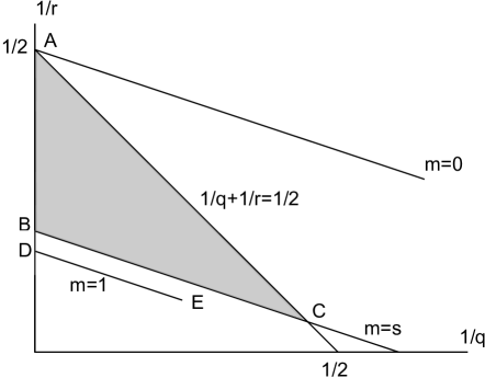
Figure 1: Region of allowed pairs

3 The Proof of Main Theorem

In this section, we will prove the main theorem. It depends on the following results.

Lemma 3.1.

If $(u_{0},u_{1})\in(\dot{H}^{s}\cap\dot{H}^{s_{p}})\times(\dot{H}^{s-1}\cap\dot{H}^{s_{p}-1})$, then we have

$$\|\nabla Iu_{0}\|_{L^{2}}\lesssim N^{1-s}\|u_{0}\|_{\dot{H}^{s}}.$$

$$\|Iu_{1}\|_{L^{2}}\lesssim N^{1-s}\|u_{1}\|_{\dot{H}^{s-1}}.$$

$$\|Iu_{0}\|_{L^{p+1}}^{p+1}\lesssim N^{2(1-s)}\|u_{0}\|_{\dot{H}^{s}}^{2}\|u_{0}\|_{\dot{H}^{s_{p}}}^{p-1}.$$

In summary, we have

$$E(Iu_{0},Iu_{1})\lesssim N^{2(1-s)}\left(\|u_{0}\|_{\dot{H}^{s}}^{2}+\|u_{1}\|_{\dot{H}^{s-1}}^{2}+\|u_{0}\|_{\dot{H}^{s}}^{2}\|u_{0}\|_{\dot{H}^{s_{p}}}^{p-1}\right).$$ (8)

Lemma 3.2.

Let $u$ be a solution of the equation (1), $J=[0,T]$, then

$$\|(u(T),\partial_{t}u(T))\|_{{\dot{H}^{s}}\times{\dot{H}^{s-1}}}\leq\|(u(0),\partial_{t}u(0))\|_{{\dot{H}^{s}}\times{\dot{H}^{s-1}}}$$

$$+C_{s,p}\left(\sup_{t\in J}E(t)^{1/2}+T\sup_{t\in J}E(t)^{\frac{p}{p+1}}+\frac{Z^{p}(J,u)}{N^{\frac{5-p}{2}+1-s}}\right).$$

Lemma 3.3.

There exist $\tau_{0}=\tau_{0}(s,p)$ and $N_{0}=N_{0}(s,p)$ such that if $|J|\leq\tau_{0}$, $N>N_{0}$ and $u(x,t)$ is a solution of the equation with

$$\sup_{t\in J}E(t)\leq 1,$$

then we have

$$Z(J,u)\lesssim_{s,p}1.$$

Lemma 3.4.

Almost Conservation Law of Energy If $u$ is a solution of the equation, then the inequality

$$|E(Iu(t_{1}))-E(Iu(t_{2}))|\lesssim\sup_{t\in J}E(t)^{1/2}\frac{Z^{p}(J,u)}{N^{(5-p)/2}}$$

holds for all times $t_{1},t_{2}\in J$.

These lemmas will be proved in the later sections. Now let us show that the main theorem holds assuming these lemmas.

Step 1: Scaling

Let $u_{\lambda}$ be

$$u_{\lambda}(x,t)=\frac{1}{\lambda^{\frac{3}{2}-s_{p}}}u(\frac{x}{\lambda},\frac{t}{\lambda}).$$ (9)

Thus

$$\partial_{t}u_{\lambda}(x,t)=\frac{1}{\lambda^{\frac{5}{2}-s_{p}}}\partial_{t}u(\frac{x}{\lambda},\frac{t}{\lambda}).$$ (10)

If $u(x,t)$ is a solution of the equation (1), one can check that $u_{\lambda}$ is still a solution of the original equation. In addition, the $\dot{H}^{s_{p}}\times\dot{H}^{s_{p}-1}$ norm is preserved under this rescaling. Using (8) we know the energy

$$E(Iu_{\lambda}(0),I\partial_{t}u_{\lambda}(0))$$

$$\lesssim N^{2(1-s)}\left(\|u_{\lambda}(0)\|_{\dot{H}^{s}}^{2}+\|\partial_{t}u_{\lambda}(0)\|_{\dot{H}^{s-1}}^{2}+\|u_{\lambda}(0)\|_{\dot{H}^{s}}^{2}\|u_{\lambda}(0)\|_{\dot{H}^{s_{p}}}^{p-1}\right)$$

$$\lesssim N^{2(1-s)}\lambda^{2s_{p}-2s}\left(\|u(0)\|_{\dot{H}^{s}}^{2}+\|\partial_{t}u(0)\|_{\dot{H}^{s-1}}^{2}+\|u(0)\|_{\dot{H}^{s}}^{2}\|u(0)\|_{\dot{H}^{s_{p}}}^{p-1}\right)$$

$$= N^{2(1-s)}\lambda^{2s_{p}-2s}\left(\|u_{0}\|_{\dot{H}^{s}}^{2}+\|u_{1}\|_{\dot{H}^{s-1}}^{2}+\|u_{0}\|_{\dot{H}^{s}}^{2}\|u_{0}\|_{\dot{H}^{s_{p}}}^{p-1}\right)$$

Let us define $C(u)$ by

$$C(u)=\|u_{0}\|_{\dot{H}^{s}}^{2}+\|u_{1}\|_{\dot{H}^{s-1}}^{2}+\|u_{0}\|_{\dot{H}^{s}}^{2}\|u_{0}\|_{\dot{H}^{s_{p}}}^{p-1},$$ (11)

and choose

$$\lambda=C_{s,p}C(u)^{\frac{1}{2(s-s_{p})}}N^{\frac{1-s}{s-s_{p}}}.$$ (12)

If $C_{s,p}$ is sufficiently large, then

$$E(Iu_{\lambda}(0),I\partial_{t}u_{\lambda}(0))\leq 1/2.$$

Step 2

We will show that the energy $E(Iu_{\lambda}(t),I\partial_{t}u_{\lambda}(t))$ is always less than $3/4$ in the whole interval $[0,\lambda T]$ if we choose sufficiently large $N=N(s,p,\|u\|,T)$. Let us define

$$T^{\prime}=\max\left\{t:t\in[0,\lambda T]\,\hbox{such that}\,E(Iu_{\lambda}(t^{\prime}),I\partial_{t}u_{\lambda}(t^{\prime}))\leq 3/4,\hbox{ for all }t^{\prime}\in[0,t]\right\}.$$

By continuity of the energy, if $T^{\prime}<\lambda T$, we have there exists $\varepsilon>0$, such that

$$E(Iu_{\lambda}(t),I\partial_{t}u_{\lambda}(t))\leq 1,\hbox{ for all }t\in[0,T^{\prime}+\varepsilon].$$

Break the interval $[0,T^{\prime}+\varepsilon]$ into subintervals $\{J_{i}\}$, $i=1,2,\cdots,n$, such that $|J_{i}|\leq\tau_{0}$. The constant $\tau_{0}=\tau_{0}(s,p)$ here and $N_{0}(s,p)$ mentioned below are the same constants as in lemma 3.3. We can always choose

$$n\leq\frac{\lambda T}{\tau_{0}}+1.$$ (13)

By lemma 3.3, we have (Let $N>N_{0}(s,p)$)

$$Z(J_{i},u_{\lambda})\lesssim 1.$$ (14)

Applying Almost Conservation Law in each subinterval, we obtain

$$E(Iu_{\lambda}(t),I\partial_{t}u_{\lambda}(t))\leq 1/2+\frac{C_{s,p}\cdot k}{N^{(5-p)/2}}.$$ (15)

for any $t\in J_{k}$. Using (13) we have for any $t\in[0,T^{\prime}+\varepsilon]$,

$$E(Iu_{\lambda}(t),I\partial_{t}u_{\lambda}(t)) \leq 1/2+\frac{C_{s,p}(1+\frac{\lambda T}{\tau_{0}})}{N^{(5-p)/2}}$$

$$\leq 1/2+\frac{C_{s,p}(1+\lambda T)}{N^{(5-p)/2}}$$

$$\leq 1/2+\frac{C_{s,p}(1+C(u)^{\frac{1}{2(s-s_{p})}}N^{\frac{1-s}{s-s_{p}}}T)}{N^{(5-p)/2}}$$

$$\leq 1/2+\frac{C_{s,p}}{N^{\frac{5-p}{2}}}+\frac{C_{s,p}C(u)^{\frac{1}{2(s-s_{p})}}T}{N^{\frac{5-p}{2}-\frac{1-s}{s-s_{p}}}}.$$

Here we use the choice of $\lambda$ (12). The constants above $C_{s,p}$ may be different in each step, but they only depend on the numbers $s,p$. Our assumption on $s$ actually implies

$$\frac{5-p}{2}>\frac{1-s}{s-s_{p}}.$$

Choosing

$$N=C\max\left\{C(u)^{\displaystyle\frac{1}{(5-p)(s-s_{p})-2(1-s)}}T^{\displaystyle\frac{1}{\frac{5-p}{2}-\frac{1-s}{s-s_{p}}}},\,N_{0}(s,p)\right\},$$ (16)

we have

$$E(Iu_{\lambda}(t),I\partial_{t}u_{\lambda}(t))\leq 3/4$$

for all $t\in[0,T^{\prime}+\varepsilon]$ if $C=C(s,p)$ is sufficiently large. This is a contradiction. Thus if we choose $N$ as (16), then the following inequality

$$E(Iu_{\lambda}(t),I\partial_{t}u_{\lambda}(t))\leq 3/4$$ (17)

holds for each $t\in[0,\lambda T]$. Breaking this interval into subintervals $J_{i}$ as above, we still have (14) and (13) holds.

Step 3

Applying lemma 3.2 to each subinterval and conducting an induction, we obtain for each $t_{0}\in[0,\lambda T]$, (Use (13), (14), (16) and (17))

$$\|(u_{\lambda}(t_{0}),\partial_{t}u_{\lambda}(t_{0}))\|_{{\dot{H}^{s}}\times{\dot{H}^{s-1}}}$$

$$\leq \|(u_{\lambda}(0),\partial_{t}u_{\lambda}(0))\|_{{\dot{H}^{s}}\times{\dot{H}^{s-1}}}+C_{s,p}\left(n+\lambda T+\frac{n}{N^{\frac{5-p}{2}+1-s}}\right)$$

$$\leq \lambda^{s_{p}-s}\|(u(0),\partial_{t}u(0))\|_{{\dot{H}^{s}}\times{\dot{H}^{s-1}}}+C_{s,p}\left(\lambda T+1+\frac{\lambda T+1}{N^{\frac{5-p}{2}+1-s}}\right)$$

$$\leq \lambda^{s_{p}-s}\|(u(0),\partial_{t}u(0))\|_{{\dot{H}^{s}}\times{\dot{H}^{s-1}}}+C_{s,p}\left(\lambda T+1\right).$$

Rescaling back we have

$$\left\|(u(\frac{t_{0}}{\lambda}),\partial_{t}u(\frac{t_{0}}{\lambda}))\right\|_{{\dot{H}^{s}}\times{\dot{H}^{s-1}}} \leq \|(u(0),\partial_{t}u(0))\|_{{\dot{H}^{s}}\times{\dot{H}^{s-1}}}+C_{s,p}\lambda^{s-s_{p}}(\lambda T+1)$$

$$\leq \|(u_{0},u_{1})\|_{{\dot{H}^{s}}\times{\dot{H}^{s-1}}}+C_{s,p}\lambda^{s-s_{p}}N^{(5-p)/2}$$

$$\leq \|(u_{0},u_{1})\|_{{\dot{H}^{s}}\times{\dot{H}^{s-1}}}+C_{s,p}C(u)^{1/2}N^{1-s}N^{(5-p)/2}$$

$$\lesssim \|(u_{0},u_{1})\|_{{\dot{H}^{s}}\times{\dot{H}^{s-1}}}+C(u)^{1/2}N^{1-s+\frac{5-p}{2}}$$

$$\lesssim \|(u_{0},u_{1})\|_{{\dot{H}^{s}}\times{\dot{H}^{s-1}}}+C(u)^{\alpha}T^{\beta}+C(u)^{1/2}.$$

The exponents $\alpha$ and $\beta$ are given by

$$\alpha=\alpha(s,p) = {\frac{\frac{5-p}{2}(1+s-s_{p})}{(5-p)(s-s_{p})-2(1-s)}};$$ (18)

$$\beta=\beta(s,p) = \frac{1-s+\frac{5-p}{2}}{\frac{5-p}{2}-\frac{1-s}{s-s_{p}}}.$$ (19)

In summary

$$\sup_{t\in[0,T]}\|(u(t),\partial_{t}u(t))\|_{{\dot{H}^{s}}\times{\dot{H}^{s-1}}}\lesssim\|(u_{0},u_{1})\|_{{\dot{H}^{s}}\times{\dot{H}^{s-1}}}+C(u)^{1/2}+C(u)^{\alpha}T^{\beta}.$$ (20)

This gives the bound for the $\dot{H}^{s}\times\dot{H}^{s-1}$ norm. We can also find an upper bound for the $\dot{H}^{s_{p}}\times\dot{H}^{s_{p}-1}$ norm as below.

The $\dot{H}^{s_{p}}\times\dot{H}^{s_{p}-1}$ Norm

By the local theory of the equation with initial data $(u_{0},u_{1})\in\dot{H}^{s}\times\dot{H}^{s-1}$, we know local solution will exist at least in the interval $[0,T_{1}]$, where the number $T_{1}$ is given by

$$T_{1}=\frac{C_{s,p}}{\|(u_{0},u_{1})\|_{\dot{H}^{s}\times\dot{H}^{s-1}}^{\frac{1}{s-s_{p}}}}.$$

This is different from the local theory with initial data in the critical space $\dot{H}^{s_{p}}\times\dot{H}^{s_{p}-1}$. In addition, Given each $s$-admissible pair $(q,r)$, we have

$$\|u\|_{L_{t}^{q}L_{x}^{r}([0,T_{1}]\times{\mathbb{R}}^{3})}\lesssim\|(u_{0},u_{1})\|_{\dot{H}^{s}\times\dot{H}^{s-1}}.$$ (21)

Now let the letter $M$ represent the upper bound as below. Please note that we can estimate $M$ by (20).

$$M=\sup_{t\in[0,T]}\|(u(t),\partial_{t}u(t))\|_{{\dot{H}^{s}}\times{\dot{H}^{s-1}}}.$$

If we break the interval $[0,T]$ into subintervals $J_{i}(i=1,2,\cdots,n)$, such that

$$|J_{i}|\leq T_{1}\approx 1/M^{\frac{1}{s-s_{p}}},$$

then the local theory can be applied in each subinterval. Choosing a specific $s$-admissible pair $(p/(1-p(s-s_{p})),6p/(5-2s_{p}))$, we have

$$\|F(u)\|_{L_{J_{i}}^{\frac{1}{1-p(s-s_{p})}}L_{x}^{\frac{6}{5-2s_{p}}}}\leq\|u\|_{L_{J_{i}}^{\frac{p}{1-p(s-s_{p})}}L_{x}^{\frac{6p}{5-2s_{p}}}}^{p}\lesssim M^{p}.$$

Thus

$$\|F(u)\|_{L_{J_{i}}^{1}L_{x}^{\frac{6}{5-2s_{p}}}}\leq|J_{i}|^{p(s-s_{p})}\|F(u)\|_{L_{J_{i}}^{\frac{1}{1-p(s-s_{p})}}L_{x}^{\frac{6}{5-2s_{p}}}}\lesssim 1.$$

The bound in question is given by a straightforward computation using the Strichartz estimates as below

$$\|(u,\partial_{t}u)\|_{C([0,T];\dot{H}^{s_{p}}\times\dot{H}^{s_{p}-1})}$$

$$\leq \|(u_{0},u_{1})\|_{\dot{H}^{s_{p}}\times\dot{H}^{s_{p}-1}}+C_{s,p}\|F(u)\|_{L_{[0,T]}^{1}L_{x}^{\frac{6}{5-2s_{p}}}}$$

$$\leq \|(u_{0},u_{1})\|_{\dot{H}^{s_{p}}\times\dot{H}^{s_{p}-1}}+C_{s,p}(1+\frac{T}{T_{1}})$$

$$\leq \|(u_{0},u_{1})\|_{\dot{H}^{s_{p}}\times\dot{H}^{s_{p}-1}}+C_{s,p}(1+TM^{\frac{1}{s-s_{p}}})$$

$$\leq \|(u_{0},u_{1})\|_{\dot{H}^{s_{p}}\times\dot{H}^{s_{p}-1}}$$

$$+C_{s,p}\left(1+T\left(\|(u_{0},u_{1})\|_{{\dot{H}^{s}}\times{\dot{H}^{s-1}}}+C(u)^{1/2}+C(u)^{\alpha}T^{\beta}\right)^{\frac{1}{s-s_{p}}}\right)$$

$$\lesssim \|(u_{0},u_{1})\|_{\dot{H}^{s_{p}}\times\dot{H}^{s_{p}-1}}+1+T\|(u_{0},u_{1})\|_{{\dot{H}^{s}}\times{\dot{H}^{s-1}}}^{\frac{1}{s-s_{p}}}+TC(u)^{\frac{1}{2(s-s_{p})}}$$

$$+C(u)^{\frac{\alpha}{s-s_{p}}}T^{\frac{\beta}{s-s_{p}}+1}.$$

4 Proof of Lemma 3.1

This lemma comes from some basic computation.

$$\|\nabla Iu_{0}\|_{L^{2}}^{2} \lesssim \int_{|\xi|\leq N}|\xi|^{2}|\hat{u_{0}}(\xi)|^{2}d\xi+\int_{|\xi|>N}|\xi|^{2}\frac{N^{2(1-s)}}{|\xi|^{2(1-s)}}|\hat{u_{0}}(\xi)|^{2}d\xi$$

$$\lesssim \int_{|\xi|\leq N}N^{2(1-s)}|\xi|^{2s}|\hat{u_{0}}(\xi)|^{2}d\xi+\int_{|\xi|>N}{N^{2(1-s)}}|\xi|^{2s}|\hat{u_{0}}(\xi)|^{2}d\xi$$

$$\lesssim N^{2(1-s)}\|u_{0}\|_{\dot{H}^{s}}^{2}.$$

Similar argument shows

$$\|Iu_{1}\|_{L^{2}}^{2}\lesssim\int_{|\xi|\leq N}|\hat{u_{1}}(\xi)|^{2}d\xi+\int_{|\xi|>N}\frac{N^{2(1-s)}}{|\xi|^{2(1-s)}}|\hat{u_{1}}(\xi)|^{2}d\xi$$

$$\lesssim \int_{|\xi|\leq N}N^{2(1-s)}|\xi|^{2(s-1)}|\hat{u_{0}}(\xi)|^{2}d\xi+\int_{|\xi|>N}{N^{2(1-s)}}|\xi|^{2(s-1)}|\hat{u_{0}}(\xi)|^{2}d\xi$$

$$\lesssim N^{2(1-s)}\|u_{1}\|_{\dot{H}^{s-1}}^{2}.$$

For the third inequality we have

$$\|Iu_{0}\|_{L^{p+1}}^{p+1} \lesssim \|Iu_{0}\|_{L^{6}}^{2}\|Iu_{0}\|_{L^{\frac{3(p-1)}{2}}}^{p-1}$$

$$\lesssim \|\nabla Iu_{0}\|_{L^{2}}^{2}\|u_{0}\|_{L^{\frac{3(p-1)}{2}}}^{p-1}$$

$$\lesssim N^{2(1-s)}\|u_{0}\|_{\dot{H}^{s}}^{2}\|u_{0}\|_{\dot{H}^{s_{p}}}^{p-1}.$$

5 Proof of Lemma 3.2

In this section we give the proof of lemma 3.2. We will first estimate the low frequency part, which is more difficult. By Strichartz estimate we have

$$\|P_{\leq 1}(u(T),\partial_{t}u(T))\|_{{\dot{H}^{s}}\times{\dot{H}^{s-1}}} \leq \|S(t)P_{\leq 1}(u(0),\partial_{t}u(0))\|_{{\dot{H}^{s}}\times{\dot{H}^{s-1}}}$$

$$+\left\|\int_{0}^{T}\frac{\sin{((T-t)\sqrt{-\Delta})}}{\sqrt{-\Delta}}P_{\leq 1}F(u(t))dt\right\|_{{\dot{H}^{s}}\times{\dot{H}^{s-1}}}$$

$$\leq \|P_{\leq 1}(u(0),\partial_{t}u(0))\|_{{\dot{H}^{s}}\times{\dot{H}^{s-1}}}+C_{s}\|P_{\leq 1}F(u)\|_{L_{J}^{1}L_{x}^{\frac{6}{5-2s}}}.$$

We can break the nonlinear part into

$$\|P_{\leq 1}F(u)\|_{L_{J}^{1}L_{x}^{\frac{6}{5-2s}}} \leq \|P_{\leq 1}F(Iu)\|_{L_{J}^{1}L_{x}^{\frac{6}{5-2s}}}+\|P_{\leq 1}[F(u)-F(Iu)]\|_{L_{J}^{1}L_{x}^{\frac{6}{5-2s}}}$$

$$\lesssim \|P_{\leq 1}F(Iu)\|_{L_{J}^{1}L_{x}^{\frac{6}{5-2s}}}+\|F(u)-F(Iu)\|_{L_{J}^{1}L_{x}^{\frac{6}{5-2s}}}$$

$$= X_{1}+X_{2},$$

and deal with each part individually

$$X_{1} \lesssim \|P_{\leq 1}F(Iu)\|_{L_{J}^{1}L_{x}^{\frac{p+1}{p}}}$$

$$\lesssim \|F(Iu)\|_{L_{J}^{1}L_{x}^{\frac{p+1}{p}}}$$

$$\lesssim T\|F(Iu)\|_{L_{J}^{\infty}L_{x}^{\frac{p+1}{p}}}$$

$$\lesssim T\sup_{t\in J}\left(\int_{{\mathbb{R}}^{3}}|F(Iu)|^{\frac{p+1}{p}}dx\right)^{\frac{p}{p+1}}$$

$$\lesssim T\sup_{t\in J}\left(\int_{{\mathbb{R}}^{3}}|Iu|^{p+1}dx\right)^{\frac{p}{p+1}}$$

$$\lesssim T\sup_{t\in J}E(t)^{\frac{p}{p+1}},$$

and (Similar argument is used in the proof of almost conservation law)

$$X_{2} \lesssim \|(|Iu|+|u|)^{p-1}|Iu-u|\|_{L_{J}^{1}L_{x}^{\frac{6}{5-2s}}}$$

$$\lesssim \|P_{\ll N}u\|_{L_{J}^{\frac{1}{\frac{7-p}{4(p-1)}+\frac{1-s}{2(p-1)}}}L_{x}^{\frac{1}{\frac{p-3}{4(p-1)}-\frac{1-s}{6(p-1)}}}}^{p-1}\cdot\|P_{\gtrsim N}u\|_{L_{J}^{\frac{1}{\frac{p-3}{4}-\frac{1-s}{2}}}L_{x}^{\frac{1}{\frac{5-p}{4}+\frac{1-s}{2}}}}$$

$$+\|P_{\gtrsim N}u\|_{L_{J}^{p}L_{x}^{\frac{6p}{5-2s}}}^{p-1}\cdot\|P_{\gtrsim N}u\|_{L_{J}^{p}L_{x}^{\frac{6p}{5-2s}}}$$

$$\lesssim \|D^{1-1}Iu\|_{L_{J}^{\frac{1}{\frac{7-p}{4(p-1)}+\frac{1-s}{2(p-1)}}}L_{x}^{\frac{1}{\frac{p-3}{4(p-1)}-\frac{1-s}{6(p-1)}}}}^{p-1}$$

$$\times\frac{1}{N^{\frac{5-p}{2}+1-s}}\|D^{1-\left(\frac{p-3}{2}-(1-s)\right)}Iu\|_{L_{J}^{\frac{1}{\frac{p-3}{4}-\frac{1-s}{2}}}L_{x}^{\frac{1}{\frac{5-p}{4}+\frac{1-s}{2}}}}$$

$$+\frac{1}{N^{\frac{5-p}{2}+1-s}}\|D^{1-\frac{3p-7+2s}{2p}}Iu\|_{L_{J}^{p}L_{x}^{\frac{6p}{5-2s}}}^{p}$$

$$\lesssim \frac{Z^{p}(J,u)}{N^{\frac{5-p}{2}+1-s}}.$$

Thus in summary we have

$$\|P_{\leq 1}(u(t),\partial_{t}u(t))\|_{{\dot{H}^{s}}\times{\dot{H}^{s-1}}} \leq \|P_{\leq 1}(u(0),\partial_{t}u(0))\|_{{\dot{H}^{s}}\times{\dot{H}^{s-1}}}$$

$$+C_{s,p}\left(T\sup_{t\in J}E(t)^{\frac{p}{p+1}}+\frac{Z^{p}(J,u)}{N^{\frac{5-p}{2}+1-s}}\right).$$

Next let us consider the high frequency part

$$\|P_{>1}u(t)\|_{\dot{H}^{s}}^{2} \leq \int_{1<|\xi|\leq 2N}|\xi|^{2s}|\hat{u}(t,\xi)|^{2}d\xi+\int_{|\xi|>2N}|\xi|^{2s}|\hat{u}(t,\xi)|^{2}d\xi$$

$$\lesssim X_{1}+X_{2}.$$

These two terms can be dominated by the energy just at the time $t$.

$$X_{1}\lesssim\int_{1<|\xi|\leq 2N}|\xi|^{2}|\hat{u}(t,\xi)|^{2}d\xi\lesssim\|\nabla Iu(t)\|_{L^{2}}^{2}\lesssim E(t).$$

$$X_{2} \lesssim \frac{1}{N^{2(1-s)}}\int_{|\xi|>2N}|\xi|^{2}\frac{N^{2(1-s)}}{|\xi|^{2(1-s)}}|\hat{u}(t,\xi)|^{2}d\xi$$

$$\lesssim \frac{1}{N^{2(1-s)}}\|\nabla Iu(t)\|_{L^{2}}^{2}$$

$$\lesssim \frac{1}{N^{2(1-s)}}E(t).$$

By similar argument we can show

$$\|P_{>1}\partial_{t}u(t)\|_{\dot{H}^{s-1}}^{2}\lesssim E(t).$$

Combining the low and high frequency parts, we have

$$\|(u(T),\partial_{t}u(T))\|_{{\dot{H}^{s}}\times{\dot{H}^{s-1}}}\leq\|(u(0),\partial_{t}u(0))\|_{{\dot{H}^{s}}\times{\dot{H}^{s-1}}}$$

$$+C_{s,p}\left(\sup_{t\in J}E(t)^{1/2}+T\sup_{t\in J}E(t)^{\frac{p}{p+1}}+\frac{Z(J,u)^{p}}{N^{\frac{5-p}{2}+1-s}}\right).$$

6 Proof of Lemma 3.3

In this section we will prove lemma 3.3.

Step 1

Let us first consider the estimate for $q=\infty$. Using the Sobolev embedding, we have

$$\|D^{1-m}Iu\|_{L_{J}^{\infty}L_{x}^{r}}\lesssim\|DIu\|_{L_{J}^{\infty}L_{x}^{2}}\lesssim\sup_{t\in J}(E(t))^{1/2}\leq 1.$$

Thus the estimate holds for $q=\infty$.

Step 2

Now we will first establish an estimate for $m\leq s$. WLOG, let $J=[0,\tau]$. Applying the operator $D^{1-m}I$ to the original equation (1) and then using the Strichartz estimate, we obtain

$$\|D^{1-m}Iu\|_{L_{J}^{q}L_{x}^{r}} \lesssim \|(D^{1-m}Iu(0),D^{1-m}I\partial_{t}u(0))\|_{\dot{H}^{m}\times\dot{H}^{m-1}}$$

$$+\|D^{1-m}IF(u)\|_{L_{J}^{1}L_{x}^{\frac{6}{5-2m}}}.$$

Using the fact $m\leq s$ we have

$$Z_{m,q,r} \lesssim \|(Iu(0),\partial_{t}Iu(0))\|_{\dot{H}^{1}\times L^{2}}+\|D^{1-m}Iu\|_{L_{J}^{\infty}L_{x}^{\frac{6}{3-2m}}}\|u\|_{L_{J}^{p-1}L_{x}^{3(p-1)}}^{p-1}$$

$$\lesssim \sup_{t\in J}E(t)^{1/2}$$

$$+ Z_{m,\infty,\frac{6}{3-2m}}\left(\tau^{\frac{5-p}{2}}\|P_{\ll N}u\|_{L_{J}^{\frac{2(p-1)}{p-3}}L_{x}^{3(p-1)}}^{p-1}+\|P_{\gtrsim N}u\|_{L_{J}^{p-1}L_{x}^{3(p-1)}}^{p-1}\right)$$

$$\lesssim \sup_{t\in J}E(t)^{1/2}+\tau^{\frac{5-p}{2}}\|D^{1-1}Iu\|_{L_{J}^{\frac{2(p-1)}{p-3}}L_{x}^{3(p-1)}}^{p-1}$$

$$+ \frac{1}{N^{\frac{5-p}{2}}}\|D^{1-{s_{p}}}Iu\|_{L_{J}^{p-1}L_{x}^{3(p-1)}}^{p-1}.$$

We also need to estimate the case when $m=1$. In this case we have

$$\|Iu\|_{L_{J}^{q}L_{x}^{r}} \lesssim \|(Iu(0),\partial_{t}Iu(0))\|_{\dot{H}^{1}\times L^{2}}+\|IF(u)\|_{L_{J}^{1}L_{x}^{2}}$$

$$\lesssim \sup_{t\in J}E(t)^{1/2}+\|D^{1-s}IF(u)\|_{L_{J}^{1}L_{x}^{\frac{6}{5-2s}}}.$$

Using the same argument as the case $m=s$, we can find the same upper bound as the previous case. In summary

$$Z(J,u)\leq C_{s,p}\left(\begin{array}[]{r}\sup_{t\in J}E(t)^{1/2}+\tau^{\frac{5-p}{2}}\|D^{1-1}Iu\|_{L_{J}^{\frac{2(p-1)}{p-3}}L_{x}^{3(p-1)}}^{p-1}\\ +\frac{1}{N^{\frac{5-p}{2}}}\|D^{1-s_{p}}Iu\|_{L_{J}^{p-1}L_{x}^{3(p-1)}}^{p-1}\end{array}\right)$$ (22)

Remark

It seems that the constant $C_{s,p}$ should have depended on $q,r$ besides $s,p$, because the best constant in a Srtrichartz estimate depends on the coefficients $(q,r)$. However, it is still possible to find a universal constant that works for each allowed triple. We can first establish individual estimates as above for those $(1/q,1/r)$ that respond to the vertices (A,B,C,D,E) in the figure 1 and then use an interpolation to gain a universal constant $C_{s,p}$ for all possible triples.

Step 3

Let

$$\tilde{Z}(t,u)=\max\left\{\|D^{1-1}Iu\|_{L_{[0,t]}^{\frac{2(p-1)}{p-3}}L_{x}^{3(p-1)}},\|D^{1-s_{p}}Iu\|_{L_{[0,t]}^{p-1}L_{x}^{3(p-1)}}\right\}.$$

This function is continuous and $\tilde{Z}(0,u)=0$. By the conclusion (22) of Step 2, we have

$$\tilde{Z}(t,u)\lesssim_{s,p}1+t^{\frac{5-p}{2}}\tilde{Z}^{p-1}(t,u)+\frac{1}{N^{\frac{5-p}{2}}}\tilde{Z}^{p-1}(t,u).$$

By a continuity argument it is clear that there exist $N_{0}(s,p)$ and $\tau_{0}(s,p)$, such that if $t<\tau_{0}$ and $N>N_{0}$, then $\tilde{Z}(t,u)\lesssim 1$. Plugging it back to (22), we finish the proof of this lemma.

7 Proof of Almost Conservation Law of Energy

In this section we will prove the almost conservation law of energy.

The Variation of the Energy

The following computation shows the difference of the energy from time $t_{1}$ to time $t_{2}$.

$$E(t_{2})-E(t_{1})=\int_{t_{1}}^{t_{2}}\partial_{t}\left[\int_{{\mathbb{R}}^{3}}(\frac{|\nabla Iu|^{2}}{2}+\frac{|\partial_{t}Iu|^{2}}{2}+\frac{|Iu|^{p+1}}{p+1})dx\right]dt$$

$$= \int_{t_{1}}^{t_{2}}\int_{{\mathbb{R}}^{3}}(\nabla Iu\cdot\partial_{t}\nabla Iu+\partial_{t}^{2}Iu\cdot\partial_{t}Iu-F(Iu)\partial_{t}Iu)dxdt$$

$$= \int_{t_{1}}^{t_{2}}\int_{{\mathbb{R}}^{3}}(\nabla Iu\cdot\partial_{t}\nabla Iu+I\Delta u\cdot\partial_{t}Iu+IF(u)\cdot\partial_{t}Iu-F(Iu)\partial_{t}Iu)dxdt$$

$$= \int_{t_{1}}^{t_{2}}\int_{{\mathbb{R}}^{3}}[\left(IF(u)-F(Iu)\right)\cdot\partial_{t}Iu]dxdt.$$

Here we use the equation (1).

The Establishment of Almost Conservation of Energy

From the computation above we can estimate the difference by the Holder’s Inequality

$$|E(Iu(t_{2}))-E(Iu(t_{1}))|\leq\|\partial_{t}Iu\|_{L_{J}^{\infty}L_{x}^{2}}\|F(Iu)-IF(u)\|_{L_{J}^{1}L_{x}^{2}}.$$

Thus

$$|E(Iu(t_{2}))-E(Iu(t_{1}))|\lesssim\sup_{t\in J}E(t)^{1/2}\|F(Iu)-IF(u)\|_{L_{J}^{1}L_{x}^{2}}.$$

The rest of the section consists of the proof of the following estimates, which immediately imply the almost conservation law.

$$\|F(Iu)-F(u)\|_{L_{J}^{1}L_{x}^{2}}\lesssim\frac{Z^{p}(J,u)}{N^{(5-p)/2}}.$$ (23)

$$\|F(u)-IF(u)\|_{L_{J}^{1}L_{x}^{2}}\lesssim\frac{Z^{p}(J,u)}{N^{(5-p)/2}}.$$ (24)

Proof of (23)

We have

$$\|F(Iu)-F(u)\|_{L_{J}^{1}L_{x}^{2}}\lesssim\|(|Iu|+|u|)^{p-1}|Iu-u|\|_{L_{J}^{1}L_{x}^{2}}$$

$$\lesssim \|P_{\ll N}u\|_{L_{J}^{\frac{4(p-1)}{7-p}}L_{x}^{\frac{4(p-1)}{p-3}}}^{p-1}\cdot\|P_{\gtrsim N}u\|_{L_{J}^{\frac{4}{p-3}}L_{x}^{\frac{4}{5-p}}}$$

$$+\|P_{\gtrsim N}u\|_{L_{J}^{p}L_{x}^{2p}}^{p-1}\cdot\|P_{\gtrsim N}u\|_{L_{J}^{p}L_{x}^{2p}}$$

$$\lesssim \|D^{1-1}Iu\|_{L_{J}^{\frac{4(p-1)}{7-p}}L_{x}^{\frac{4(p-1)}{p-3}}}^{p-1}\cdot\frac{1}{N^{(5-p)/2}}\|D^{1-\frac{p-3}{2}}Iu\|_{L_{J}^{\frac{4}{p-3}}L_{x}^{\frac{4}{5-p}}}$$

$$+\frac{1}{N^{(5-p)/2}}\|D^{1-\frac{3p-5}{2p}}Iu\|_{L_{J}^{p}L_{x}^{2p}}^{p}$$

$$\lesssim \frac{Z^{p}(J,u)}{N^{(5-p)/2}}.$$

Here we used the inequality

$$s>\frac{p-3}{2},\frac{3p-5}{2p}.$$

Proof of (24)

For the second inequality

$$\|F(u)-IF(u)\|_{L_{J}^{1}L_{x}^{2}}$$

$$\lesssim \|P_{\gtrsim N}F(u)\|_{L_{J}^{1}L_{x}^{2}}$$

$$\lesssim \|P_{\gtrsim N}F(P_{\ll N}u)\|_{L_{J}^{1}L_{x}^{2}}+\|P_{\gtrsim N}[F(u)-F(P_{\ll N}u)]\|_{L_{J}^{1}L_{x}^{2}}$$

$$\lesssim \|P_{\gtrsim N}F(P_{\ll N}u)\|_{L_{J}^{1}L_{x}^{2}}+\|F(u)-F(P_{\ll N}u)\|_{L_{J}^{1}L_{x}^{2}}$$

$$\lesssim \|P_{\gtrsim N}F(P_{\ll N}u)\|_{L_{J}^{1}L_{x}^{2}}+\left\||P_{\ll N}u|^{p-1}P_{\gtrsim N}u\right\|_{L_{J}^{1}L_{x}^{2}}$$

$$+\left\||P_{\gtrsim N}u|^{p-1}P_{\gtrsim N}u\right\|_{L_{J}^{1}L_{x}^{2}}$$

$$\lesssim X_{1}+X_{2}+X_{3}.$$

The last two terms $X_{2}$ and $X_{3}$ can be estimated in the same way as in the proof of (23), thus we only need to consider the first term here.

$$X_{1} \lesssim \frac{1}{N^{(5-p)/2}}\|D^{\frac{5-p}{2}}F(P_{\ll N}u)\|_{L_{J}^{1}L_{x}^{2}}$$

$$\lesssim \frac{1}{N^{(5-p)/2}}\|P_{\ll N}u\|_{L_{J}^{\frac{4(p-1)}{7-p}}L_{x}^{\frac{4(p-1)}{p-3}}}^{p-1}\cdot\|D^{\frac{5-p}{2}}P_{\ll N}u\|_{L_{J}^{\frac{4}{p-3}}L_{x}^{\frac{4}{5-p}}}$$

$$\lesssim \frac{1}{N^{(5-p)/2}}\|D^{1-1}Iu\|_{L_{J}^{\frac{4(p-1)}{7-p}}L_{x}^{\frac{4(p-1)}{p-3}}}^{p-1}\cdot\|D^{1-\frac{p-3}{2}}Iu\|_{L_{J}^{\frac{4}{p-3}}L_{x}^{\frac{4}{5-p}}}$$

$$\lesssim \frac{Z^{p}(J,u)}{N^{(5-p)/2}}.$$

References

- [1] J. Colliander, M. Keel, S. Staffilani, H. Takaoka and T. Tao, Almost Conservation Laws and Global Rough Solutions to a Nonlinear Schrödinger Equation, Mathematical Research Letters 9, 659-682(2002).
- [2] J. Ginibre and G. Velo, Generalized Strichartz inequality for the wave equation, Journal of functional analysis 133(1995), 50-68.
- [3] M. Keel, T. Roy and T. Tao, Global Well-Posedness of the Maxwell-Klein-Gordon equation below the energy norm, Discrete and Continuous Dynamical Systems 30(2011), 573 - 621.
- [4] S. Kwon and T. Roy, Generation of decay estimate and Application to scattering of rough solutions of 3D NLKG, arXiv: 1008.0094v1.
- [5] T. Roy, Global Well-posedness for the radial defocusing cubic wave equation in and for rough data, arXiv: 0708.2299v3.
- [6] T. Roy, Introduction to Scattering for Radial 3D NLKG Below Energy Norm, Journal of Differential Equations 248(2010), 893-923.
- [7] T. Roy, On control of Sobolev Norms for some Semilinear Wave Equation with Localized Data, arXiv: 1204.3038v1.
- [8] T. Tao, M. Visan and X. Zhang, The Nonlinear Schrödinger Equation With Combined Power-Type Nonlinearities, Communications in Partial Differential Equations 32(2007), 1281-1343.