Superfluid stiffness renormalization and critical temperature enhancement in a composite superconductor

Abstract

We study a model of a composite system constructed from a ”pairing layer” of disconnected attractive-$U$ Hubbard sites that is coupled by single-particle tunneling, $t_{\perp}$, to a disordered metallic layer. For small inter-layer tunneling the system is described by an effective long-range $XY$ phase model whose critical temperature, $T_{c}$, is essentially insensitive to the disorder and is exponentially suppressed by quantum fluctuations. $T_{c}$ reaches a maximum for intermediate values of $t_{\perp}$, which we calculate using a combination of mean-field, classical and quantum Monte Carlo methods. The maximal $T_{c}$ scales as a fraction of the zero temperature gap of the attractive sites when $U$ is smaller than the metallic bandwidth, and is bounded by the maximal $T_{c}$ of the two-dimensional attractive Hubbard model for large $U$. Our results indicate that a thin, rather than a thick, metallic coating is better suited for the enhancement of $T_{c}$ at the surface of a phase fluctuating superconductor.

I Introduction

Recently, composite systems made of a metal overlaying a superconductor with low phase stiffness have received theoretical attentionOurs ; Okamoto ; Ehud after experiments have demonstrated that the superconducting transition temperature, $T_{c}$, can be enhanced in bilayers consisting of underdoped and overdoped cuprates.Yuli ; Gozar In particular, Ref. Ours, considered a model of a pairing layer with zero phase stiffness, constructed from disconnected attractive-$U$ Hubbard sites, that is coupled via single-particle tunneling $t_{\perp}$ to a metallic noninteracting layer. As $t_{\perp}$ increases from zero, phase coupling between the pairing sites is established by Josephson tunneling through the metallic layer. At the same time, however, the pairing strength is diminished owing to the proximity effect induced by the same delocalization events. Consequently, $T_{c}$ reaches a maximum at an intermediate value of $t_{\perp}$, where both these trends attain a simultaneous optimum. It was shown, within a mean-field approximation, that the maximal $T_{c}$ approaches the limit set by the pairing scale of the Hubbard sites when the metallic bandwidth, $8t$, is much larger than $U$. Here we wish to reexamine these results using more accurate analytical and numerical techniques.

An additional goal of the present work is to study the effects of disorder in the metallic layer on $T_{c}$. Owing to Andersonanderson , it is well known that $T_{c}$ of a dirty BCS $s$-wave superconductor is essentially insensitive to disorder as long as $T_{c}$ is much larger than the local mean level spacing. However, BCS theory ignores fluctuations in the superconducting order parameter and one expects deviations from Anderson’s result when fluctuations are large. Indeed, phase fluctuations dominate the physics in strongly disordered and granular systems,Ma ; Fisher ; chak ; Ghosal98 ; Beloborodov ; Dubi ; borissteve where they can reduce $T_{c}$ to zero. In the bilayer that we study the disorder resides away from the pairing sites and is therefore expected to have only mild consequences for pairing. However, since phase stiffness is established by Josephson tunneling through the metal it is interesting to study the manner in which it is affected by the random potential.

Our results indicate that although the general picture obtained in Ref. Ours, holds, it requires some modifications. First, the analysis of Ref. Ours, relied on a Bogoliubov de-Gennes (BdG) mean-field treatment to calculate the phase stiffness. While this approximation takes into account the suppression of the phase stiffness by thermally excited quasiparticles, it ignores the renormalization of the stiffness by thermal and quantum phase fluctuations. The latter have little effect in the nearest-neighbor $XY$ model and the two-dimensional attractive Hubbard modelPaiva04 , where using the unrenormailzed stiffness reproduces the correct $T_{c}$ to within 40%. We show that this is not the case in the presence of long range phase couplings. Such couplings, which extend up to the thermal length of the metal, occur in the small $t_{\perp}$ regime of the bilayer. Under these circumstances classical phase fluctuations on scales smaller than the thermal length lead to a rapid decrease of the stiffness and therefore to a much lower $T_{c}$ than is anticipated from the unrenormalized stiffness. Even more important are the quantum phase fluctuations in the small $t_{\perp}$ regime, which lead to an exponential suppression of $T_{c}$ relative to its mean-field value.

Secondly, using quantum Monte Carlo and classical Monte Carlo mean-field techniques we find that the highest $T_{c}$ (maximized over $t_{\perp}$), is smaller by a factor 3-4 than the mean-field prediction for small and intermediate $U/t$. For large $U/t$ it is bounded by the maximal $T_{c}$ of the two-dimensional attractive Hubbard model. Our calculations reveal that the maximum is largely governed by classical phase fluctuations.

For small inter-layer tunneling the primary effect of the disorder is to decrease the range over which coherent phase coupling is mediated through the metal. However, as long as the metal remains in the diffusive regime, this has a negligible effect on $T_{c}$. Using a mean-field approach to estimate the effects of disorder away from the small $t_{\perp}$ regime yields a weak correction to the maximal $T_{c}$ at small disorder strength. Nevertheless, once the disorder becomes large in comparison to the hopping amplitude in the metallic layer the maximal $T_{c}$ is significantly suppressed. We conclude the paper with a short discussion of the relevance of these insights to attempts to enhance $T_{c}$ at the surface of a phase fluctuating superconductor.

II The model and its analysis in the small $t_{\perp}$ limit

II.1 The model

We consider a bilayer, see Fig. 1, consisting of a noninteracting disordered upper layer and a lower layer of disconnected negative-$U$ Hubbard sites. Each layer contains $N=L^{2}/a^{2}$ sites in a square array with lattice constant $a$. Neighboring sites on the two layers are connected via single particle tunneling, $t_{\perp}$. We denote by $c_{i\sigma}$ and $f_{i\sigma}$ the annihilation operator of an electron with spin $\sigma$ on the $i$th site of the upper and lower layer, respectively. The imaginary time action describing the model is

$$\!\!\!\!\!\!S\!\!\!\! =\int_{0}^{\beta}d\tau\left[\sum_{i,\sigma}c_{i\sigma}^{\dagger}\left(\partial_{\tau}-\mu+\epsilon+V_{i}\right)c_{i\sigma}\right.$$ (1)

$$-\;t\sum_{\left\langle i,j\right\rangle,\sigma}\left(c_{i\sigma}^{\dagger}c_{j\sigma}+{\rm H.c.}\right)+\sum_{i,\sigma}f_{i\sigma}^{\dagger}\left(\partial_{\tau}-\mu\right)f_{i\sigma}$$

$$-\left.U\sum_{i}f_{i\uparrow}^{\dagger}f_{i\uparrow}f_{i\downarrow}^{\dagger}f_{i\downarrow}-t_{\perp}\sum_{i,\sigma}\left(c_{i\sigma}^{\dagger}f_{i\sigma}+{\rm H.c.}\right)\right].$$

Here $\beta=1/T$ is the inverse temperature, $\mu$ is the chemical potential and $t$ is the hopping amplitude between sites in the upper layer, which contains a Gaussian random potential $V$ and a constant potential $\epsilon$ used to adjust the Fermi energy away from any van-Hove singularities.

II.2 Phase-only action

We proceed by decoupling the interaction term using a Hubbard-Stratonovich transformation $-Uf_{i\uparrow}^{\dagger}f_{i\downarrow}^{\dagger}f_{i\downarrow}f_{i\uparrow}\rightarrow\Delta^{*}_{i}\Delta_{i}/U+\Delta_{i}^{*}f_{i\downarrow}f_{i\uparrow}+\Delta_{i}f^{\dagger}_{i\uparrow}f^{\dagger}_{i\downarrow}$, where $\Delta_{i}=|\Delta_{i}|e^{i\theta_{i}}$. Gauge transforming $f_{i\sigma}\rightarrow f_{i\sigma}e^{i\theta_{i}/2}$, integrating out the noninteracting layer and denoting $\Psi_{i}^{\dagger}=(f_{i\uparrow}^{\dagger},f_{i\downarrow})$ leads to

$$S = \int_{0}^{\beta}d\tau d\tau^{\prime}\sum_{ij}\Psi_{i}^{\dagger}(\tau)[M^{(0)}+V^{(0)}+V^{(1)}]\Psi_{j}(\tau^{\prime})$$ (2)

$$+ \int_{0}^{\beta}d\tau\sum_{i}|\Delta_{i}(\tau)|^{2},$$

with

$$M^{(0)} = [\partial_{\tau}{\bf I}-\mu\mbox{\boldmath$\sigma$}_{3}+|\Delta_{i}(\tau)|\mbox{\boldmath$\sigma$}_{1}]\delta_{ij}\delta(\tau-\tau^{\prime}),$$

$$V^{(0)} = \frac{i}{2}\partial_{\tau}\theta_{i}(\tau)\mbox{\boldmath$\sigma$}_{3}\delta_{ij}\delta(\tau-\tau^{\prime}),$$

$$V^{(1)} = t_{\perp}^{2}e^{-i[\theta_{i}(\tau)-\theta_{j}(\tau^{\prime})]/2}{\cal G}_{ij}(\tau-\tau^{\prime})\mbox{\boldmath$\sigma$}_{3},$$ (3)

where ${\cal G}_{ij}(\tau)$ is the Green’s function of the noninteracting layer, and $\sigma$ are the Pauli matrices.

Next, we integrate out the degrees of freedom of the pairing layer. We do so perturbatively to second order in $V^{(0)}$ and $V^{(1)}$. The time independent amplitude $|\Delta_{i}|\equiv|\Delta_{i}|(\Omega_{n}=0)$ is essentially set by the zeroth order contribution $(\beta/U)\sum_{i}|\Delta_{i}|^{2}-{\rm Tr}\ln M^{(0)}(|\Delta_{i}|)$ to the effective action, which provides within a saddle point approximation the BCS gap equation for the decoupled Hubbard sites. We assume that the pairing layer is close to half filling such that $\mu\ll|\Delta|$, and obtain as a result the $T=0$ solution $|\Delta|\equiv\Delta_{0}\approx U/2$. The ${\cal O}(t_{\perp}^{2})$ contribution modifies the gap equation and leads to a reduction of order $t_{\perp}^{2}/t$ of $\Delta_{0}$, reflecting the proximity effect. In the following we assume that $t_{\perp}^{2}/t,T\ll\Delta_{0}$ and therefore neglect both this effect and any thermal or quantum fluctuations of the gap amplitude.

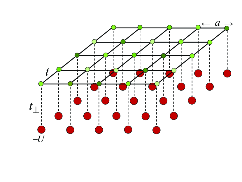
Figure 1: The model: A square lattice of disconnected attractive-$U$ Hubbard sites is coupled via single-particle tunneling $t_{\perp}$ to a noninteracting tight-binding layer with on-site random disorder.

The action governing the phase fluctuations is derived in the appendix. There we show that its dominant terms are

$$\!\!\!\!\!\!\!S_{\theta} = \frac{1}{8\Delta_{0}}\int_{0}^{\beta}d\tau\sum_{i}(\partial_{\tau}\theta_{i})^{2}$$ (4)

$$- \int_{0}^{\beta}d\tau d\tau^{\prime}\sum_{i,j}K(r_{ij},\tau-\tau^{\prime})\cos[\theta_{i}(\tau)-\theta_{j}(\tau^{\prime})].$$

The Kernel $K(r,\tau)$ decays exponentially for spatial separations $r_{ij}=|{\bf r}_{i}-{\bf r}_{j}|$ larger than the thermal length $l_{T}$. This decay reflects the loss of coherence between the dynamical phases of the members of a pair that mediates the phase coupling. Due to thermal smearing of the Fermi-Dirac distribution the difference between the energies of the two electrons is of order $T$, which leads to loss of coherence after time $1/T$. In the clean limit where the elastic mean free time of the metal satisfies $\tau_{e}^{-1}\ll T$ this coherence time translates to a distance $l_{T}=v_{F}/T$ covered by the ballistically propagating electrons with Fermi velocity $v_{F}$. In the same clean limit we find for $l_{T}\gg r\gg\xi=v_{F}/\Delta_{0}$, that the kernel is

$$K(l_{T}\gg r\gg\xi,\tau)=\frac{t_{\perp}^{4}N_{F}a^{4}}{2\pi^{2}v_{F}}\frac{1}{r}\frac{1}{(\Delta_{0}\tau)^{2}+(r/\xi)^{2}},$$ (5)

where $N_{F}$ is the density of states of the metallic layer at the Fermi energy. Up to logarithmic corrections the behavior at shorter distances may be approximated by

$$\!\!K(\xi\gg r\gg a,\tau) = \frac{t_{\perp}^{4}N_{F}a^{4}}{2\pi^{2}v_{F}}\frac{1}{r}$$ (6)

$$\times \left[\frac{\pi^{2}}{4}e^{-2\Delta_{0}|\tau|}+\frac{(\Delta_{0}\tau)^{2}}{1+(\Delta_{0}\tau)^{4}}\right].$$

Owing to the reasons outlined above the phase coupling in the diffusive regime $\tau_{e}^{-1}\gg T$ exhibits a similar exponential decay beyond the thermal length, which for a disordered metal with diffusion constant $D$ is given by $l_{T}=\sqrt{D/T}$. In the important range $l_{T}\gg r\gg\xi=\sqrt{D/\Delta_{0}}$ the kernel behaves to within logarithmic accuracy as

$$K(l_{T}\gg r\gg\xi,\tau)=\frac{t_{\perp}^{4}N_{F}a^{4}}{2\pi^{2}D}\frac{1}{(\Delta_{0}\tau)^{2}+(r/2\xi)^{4}}.$$ (7)

II.3 Classical phase fluctuations

In the small $t_{\perp}$ limit the superconducting critical temperature, $T_{c}$, equals the phase ordering temperature as determined by the action, Eq. (4). Being a finite temperature transition in a two-dimensional system with finite range couplings it is clear that the phase ordering transition belongs to the classical Berezinskii-Kosterlitz-Thouless (BKT) universality class. However, $T_{c}$ itself is determined by both quantum (time-dependent) and classical (time-independent) phase fluctuations. As we shall see, the quantum phase fluctuations can not be neglected and are in fact dominant for small $t_{\perp}$, leading to exponential suppression of $T_{c}$. Albeit, we begin by considering the effects of the classical fluctuations. We do so since the treatment of the classical fluctuations will reveal a lesson concerning the renormalization of the phase stiffness which is generic to models with interactions that extend well beyond nearest neighbors and since it will provide the tool to calculate the effects of the quantum fluctuations.

To this end, consider the case of a time-independent but space fluctuating $\theta$. Assuming $\beta\Delta_{0}\gg 1$ and carrying out the time integration in Eq. (4) results in

$$S_{\rm class}=-\beta\frac{t_{\perp}^{4}N_{F}a^{2}}{\Delta_{0}^{2}}\sum_{i,j}f(r_{ij})\cos(\theta_{i}-\theta_{j}),$$ (8)

with phase couplings $f(r)$ given by

$$\begin{array}[]{ccc}&{\rm clean\;limit}&{\rm diffusive\;limit}\\ \xi\gg r\gg a,l_{e}&\frac{a^{2}}{4\xi r}&-\frac{1}{4}\left(\frac{a}{\xi}\right)^{2}\ln\left(\frac{e^{\gamma-1/2}}{\sqrt{2}}\frac{r}{\xi}\right)\\ \\ \l_{T}\gg r\gg\xi&\frac{1}{2\pi}\left(\frac{a}{r}\right)^{2}&\frac{1}{\pi}\left(\frac{a}{r}\right)^{2}\\ \\ r\gg l_{T}&\frac{2a^{2}}{l_{T}r}e^{-2\pi r/l_{T}}&\left(\frac{a}{l_{T}}\right)^{\frac{3}{2}}\frac{(2\pi)^{1/4}}{\sqrt{r/a}}e^{-\sqrt{2\pi}\,r/l_{T}},\end{array}$$ (15)

where $l_{e}=v_{F}\tau_{e}$ is the elastic mean free path and $\gamma$ is the Euler constant. In our region of interest $T\ll\Delta_{0}$ and the physics is governed by the couplings in the range $l_{T}\gg r\gg\xi$. Thus, we are led to study the following $XY$-type model

$$H=-\frac{J}{2}\sum_{i,j}\left(\frac{a}{r_{ij}}\right)^{2}e^{-r_{ij}/\lambda}\cos(\theta_{i}-\theta_{j}),$$ (16)

with $J\sim t_{\perp}^{4}N_{F}a^{2}/\Delta_{0}^{2}$ and $\lambda\sim l_{T}$ as an effective description of the classical phase fluctuations. Here, for sake of simplicity, we extended the $r^{-2}$ behavior of the coupling down to the short distance cutoff, ignoring the crossover when $r<\xi$, see Eq. (15). As we shall demonstrate, this leads to a negligible correction to $T_{c}$.

Since the phase ordering transition belongs to the BKT class its critical temperature is related to the universal jump of the renormalized phase stiffness at criticality:

$$\rho_{s}(T_{c})=\frac{2}{\pi}T_{c}.$$ (17)

In turn, the phase stiffness is calculated from the free energy in the presence of a phase twist, $\phi$, per bond in the $x$ direction. That is, if $H=-(1/2)\sum_{i,j}J_{ij}\cos[\theta_{i}-\theta_{j}+(x_{i}-x_{j})\phi/a]$ then

$$\!\!\!\!\!\!\!\!\!\!\!\!\!\!\!\!\rho_{s}(T)=\left.\left(\frac{a}{L}\right)^{2}\frac{\partial^{2}F}{\partial\phi^{2}}\right|_{\phi=0}$$

$$=\frac{1}{2L^{2}}{\Bigg{\{}}{\Bigg{\langle}}\sum_{i,j}(x_{i}-x_{j})^{2}J_{ij}\cos(\theta_{i}-\theta_{j}){\Bigg{\rangle}}$$

$$-\frac{1}{2T}{\Bigg{\langle}}{\Bigg{[}}\sum_{i,j}(x_{i}-x_{j})J_{ij}\sin(\theta_{i}-\theta_{j}){\Bigg{]}}^{2}{\Bigg{\rangle}}{\Bigg{\}}},$$ (18)

where here $\langle\rangle$ denotes thermal averaging.

For the standard $XY$ model it is known that the BKT criterion (17) yields a fair estimate for $T_{c}$ even when $\rho_{s}$ is replaced by the bare stiffness $\rho_{s}^{0}$, unrenormalized by vortices and longitudinal phase fluctuations. Indeed, for that model $\rho_{s}^{0}=J$, as calculated from Eq. (II.3) using a uniform phase field $\theta_{i}=\theta$. This gives the estimate $T_{c}=(\pi/2)J$, which is to be compared with the most recent numerical valueHasen05 $T_{c}=0.8929J$. One may, therefore, attempt to apply the same approximation to calculate the transition temperature of model (16). For this case one finds, using the fact $\lambda\gg a$, that

$$\rho_{s}^{0}=\frac{J}{2a^{2}}\int d^{2}r\left(\frac{x}{r}\right)^{2}e^{-r/\lambda}=\frac{\pi}{2}\left(\frac{\lambda}{a}\right)^{2}J,$$ (19)

and the estimate $T_{c}=(\pi\lambda/2a)^{2}J$. Accordingly, the temperature dependence of $\lambda\sim l_{T}$ would imply $T_{c}\sim t_{\perp}^{2}/\Delta_{0}$ for the diffusive system and $T_{c}\sim(t_{\perp}^{4}N_{F}v_{F}^{2}/\Delta_{0}^{2})^{1/3}$ in the clean limit. The latter result was previously derived in Ref. Ours, within the same approximation.

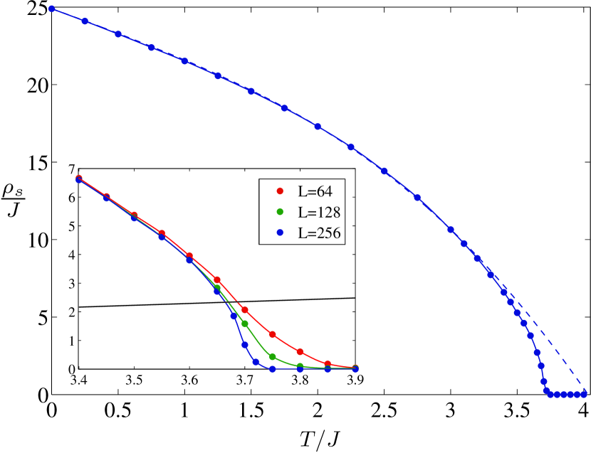
Figure 2: The phase stiffness of the effective model, Eq. (16), with $\lambda/a=4$. The dashed line is a fit (with $\lambda/a=3.897$, ${\bar{J}}/J=0.108$ and $z=8$) using the mean-field approximation discussed in the text. The inset shows the size dependence of $\rho_{s}$ in the vicinity of the transition, which occurs near the crossing of the stiffness curves with the solid black line $\rho_{s}=(2/\pi)T$.

To test the validity of these estimates we calculated $\rho_{s}(T)$ for the Hamiltonian, Eq. (16), via Monte-Carlo simulations of systems with up to $L=512$. For this purpose we used Eq. (II.3) and implemented the Wolff algorithmWolff , which is easily generalized to include couplings beyond nearest-neighbor range. Our results, see Fig. 2, indicate that the phase stiffness develops a discontinuity, in accord with the expected signature at a BKT transition. However, unlike the situation in the standard $XY$ model, $\rho_{s}(T_{c})$ is massively renormalized down from its bare ($T=0$) value $\rho_{s}^{0}$. In fact, as shown by Fig. 3, this renormalization leads in our region of interest $\lambda/d\gg 1$ to $T_{c}\simeq 3.21J\ln(0.74\lambda/a)$ instead of $T_{c}\sim J(\lambda/a)^{2}$. Therefore, using the above stated values of $J$ and $\lambda$ in terms of the parameters of the original model we find the following estimate for $T_{c}$, based on thermal fluctuations alone

$$T_{c,{\rm class}}\sim\frac{N_{F}a^{2}t_{\perp}^{4}}{\Delta_{0}^{2}}\ln\left(\frac{\sqrt{N_{F}\eta}\Delta_{0}}{N_{F}a^{2}t_{\perp}^{2}}\right)+{\cal O}\left(t_{\perp}^{4}\ln\ln t_{\perp}^{-1}\right),$$ (20)

where $\eta=D,v_{F}a$ in the diffusive and ballistic regimes, respectively.

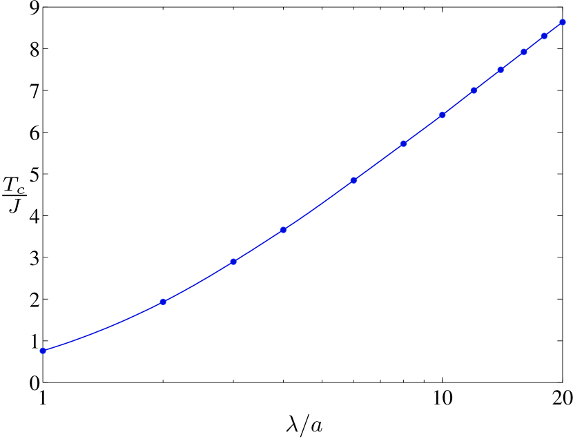
Figure 3: The critical temperature of the effective model, Eq. (16), as function of $\lambda/a$.

In order to acquire an insight into these findings let us consider the following coarse-grained model where we divide the system into blocks containing $(\lambda/a)^{2}$ unit spins. Each spin is assumed to interact with all the other spins in its own block and in the $z$ neighboring blocks. To make analytical progress we replace the original coupling in our model, which decays as $1/r^{2}$, by its average over a block. Hence, if we denote by $\mathbf{s}_{i}^{I}$, $i=1\ldots(\lambda/a)^{2}$, the spins on the $I$th block, and by $\mathbf{m}_{I}=\sum_{i}\mathbf{s}_{i}^{I}$ the total (super)spin on that block, we are led to study the model

$${\bar{H}}=-\frac{\bar{J}}{2}\sum_{I}\mathbf{m}_{I}^{2}-{\bar{J}}\sum_{\langle I,J\rangle}\mathbf{m}_{I}\cdot\mathbf{m}_{J},$$ (21)

where $\langle I,J\rangle$ denotes the blocks that couple to block $I$ and

$${\bar{J}}\approx J\left(\frac{a}{\lambda}\right)^{2}\int_{a}^{\infty}d^{2}r\,\frac{e^{-r/\lambda}}{r^{2}}\approx J\left(\frac{a}{\lambda}\right)^{2}\ln\left(\frac{\lambda}{a}\right).$$ (22)

The coarse-grained model, Eq. (21), is a model of soft superspins whose average length $M=\langle|\mathbf{m}|\rangle$ is determined by the intra-block phase fluctuations. As long as fluctuations in $M$ are ignored the system can be viewed as an ordinary $XY$ model for unit superspins with coupling ${\bar{J}}M^{2}$. Hence, we are interested in calculating the temperature dependence of the latter. To this end, we continue to treat the intra-block fluctuations exactly but treat the inter-block coupling in mean-field approximation using the following effective single block Hamiltonian

$${\bar{H}}_{MF}=-\frac{\bar{J}}{2}\mathbf{m}^{2}-{\bar{J}}z\mathbf{M}\cdot\mathbf{m},$$ (23)

with the self-consistency condition $\mathbf{M}=\langle\mathbf{m}\rangle_{{\bar{H}}_{MF}}$.

Using the Hubbard-Stratonovich transformationAntoni

$$e^{\beta{\bar{J}}\mathbf{m}^{2}/2}=\frac{1}{\pi}\int_{-\infty}^{\infty}d^{2}ye^{-\mathbf{y}^{2}+\sqrt{2\beta{\bar{J}}}\mathbf{m}\cdot\mathbf{y}},$$ (24)

we are able to write the mean-field partition function as

$$Z_{MF}=\int_{-\infty}^{\infty}\frac{d^{2}y}{\pi}\prod_{i=1}^{(\lambda/a)^{2}}\int_{0}^{2\pi}d\phi_{i}e^{-\mathbf{y}^{2}+|\mathbf{x}|\cos\phi_{i}},$$ (25)

where $\phi_{i}$ is the angle between $\mathbf{s}_{i}$ and $\mathbf{x}=\sqrt{2\beta{\bar{J}}}\mathbf{y}+z\beta{\bar{J}}\mathbf{M}$. Carrying out the integrations over the $\phi_{i}$s and the direction of $\mathbf{x}$ we arrive at

$$\!\!\!\!\!\!\!\!\!\!\!\!\!\!Z_{MF}=\frac{(2\pi)^{(\lambda/a)^{2}}}{\beta{\bar{J}}}e^{\beta{\bar{J}}z^{2}M^{2}/2}$$

$$\times\int_{0}^{\infty}dx\,x\left[I_{0}(x)\right]^{(\lambda/a)^{2}}I_{0}(zMx)e^{-x^{2}/(2\beta{\bar{J}})},$$ (26)

where $I_{0}(x)$ is the modified Bessel function of the first kind. Finally, the self-consistency condition implies $M^{2}=(\beta{\bar{J}})^{-1}\partial\ln Z_{MF}/\partial z$, from which follows

$$M\!=\frac{1}{(1+z)\beta{\bar{J}}}\frac{\int_{0}^{\infty}\!dxx^{2}\left[I_{0}(x)\right]^{(\lambda/a)^{2}}\!I_{1}(zMx)e^{-x^{2}/(2\beta{\bar{J}})}}{\int_{0}^{\infty}\!dxx\left[I_{0}(x)\right]^{(\lambda/a)^{2}}\!I_{0}(zMx)e^{-x^{2}/(2\beta{\bar{J}})}}.$$ (27)

Near the mean-field transition temperature, $T_{c,MF}$, $M\rightarrow 0$ and we may approximate $I_{0}(zMx)\approx 1$ and $I_{1}(zMx)\approx zMx$. This, together with the parameterization $\beta_{c}{\bar{J}}=c(a/\lambda)^{2}$ for the inverse critical temperature, turns Eq. (27) into

$$1=\frac{z}{1+z}\frac{\int_{0}^{\infty}dxx^{3}\left[I_{0}\left(\sqrt{2c}(a/\lambda)x\right)\right]^{(\lambda/a)^{2}}e^{-x^{2}}}{\int_{0}^{\infty}dxx\left[I_{0}\left(\sqrt{2c}(a/\lambda)x\right)\right]^{(\lambda/a)^{2}}e^{-x^{2}}}.$$ (28)

Since $I_{0}(x\ll 1)\approx 1+x^{2}/4$ one finds in the limit $a/\lambda\ll 1$ that $\left[I_{0}\left(\sqrt{2c}(a/\lambda)x\right)\right]^{(\lambda/a)^{2}}\approx e^{cx^{2}/2}$. The integrals in Eq. (28) are then readily evaluated with the result $c=2/(1+z)$, leading to

$$T_{c,MF}=\frac{1+z}{2}\left(\frac{\lambda}{a}\right)^{2}{\bar{J}}\sim J\ln(\lambda/a).$$ (29)

The phase stiffness of the coarse-grained model is determined by two types of processes: intra-block fluctuations that reduce $M$ and with it the average coupling between superspins, and inter-block fluctuations of the superspins. Our mean-field treatment ignores the second type of fluctuations. Fig. 2 depicts a fit to $\rho_{s}(T)/J$ of Hamiltonian (16) using $M^{2}(T)$ obtained by solving Eq. (27). The fit begins to deviate from $\rho_{s}(T)$ as the latter becomes of order $(2/\pi)T$. Hence, the following physical picture emerges: The phase stiffness is rapidly reduced from its large bare value by fluctuations on scales smaller than $\lambda$. These include both longitudinal and transverse vortex excitations which reach, according to our numerical findings, much higher densities below $T_{c}$ as compared to the case of the standard $XY$ model. It is this renormalization that is responsible for the $T_{c}$ scaling with $\ln(\lambda/a)$. Once $\rho_{s}$ approaches $(2/\pi)T$ vortex fluctuations on scales larger that $\lambda$ become important and drive the system through a BKT transition.

Before proceeding to discuss the quantum fluctuations let us consider the approximation we made in neglecting the crossover to a slower decay of the coupling, Eq. (15), for $r<\xi$. Based on the insights gathered above we can easily modify the mean-field treatment to include this crossover by defining the average coupling according to

$${\bar{J}} \approx J\left(\frac{a}{\lambda}\right)^{2}\left[\int_{a}^{\xi}d^{2}r\,\frac{e^{-r/\lambda}}{\xi r}+\int_{\xi}^{\infty}d^{2}r\,\frac{e^{-r/\lambda}}{r^{2}}\right]$$ (30)

$$\approx J\left(\frac{a}{\lambda}\right)^{2}\left[1+\ln\left(\frac{\lambda}{\xi}\right)\right].$$

Since $\lambda\gg\xi$ this introduces only a small correction to the mean-field transition temperature, Eq. (29).

II.4 Quantum phase fluctuations

For small $t_{\perp}$ the short time phase dynamics on a single site is governed by the first term in the action (4), which implies

$$\langle e^{-i[\theta_{i}(\tau)-\theta_{i}(\tau^{\prime})]}\rangle=e^{-2\Delta_{0}|\tau-\tau^{\prime}|}.$$ (31)

This means that a site phase is essentially constant over a time of the order of $\Delta_{0}^{-1}$ and allows us to coarse grain space-time into ”needles” of length $\Delta_{0}^{-1}$ in the imaginary time direction. The phases of the needles interact according to the last term in Eq. (4), resulting in a coarse grained phase action

$$S_{\theta}=-\sum_{\tau,\tau^{\prime}}\sum_{i,j}g(r_{ij},\tau-\tau^{\prime})\cos[\theta_{i}(\tau)-\theta_{j}(\tau^{\prime})],$$ (32)

where $g(r,\tau)=\Delta_{0}^{-2}K(r,\tau)$, and $\theta_{i}(\tau)$ denotes the phase of the needle centered around time $\tau$ at site $i$.

The fact that $g(r,\tau)$ is long ranged in the time direction allows us to apply a similar mean-field approach to the one employed above in order to estimate $T_{c}$. Now, however, we include the effects of both quantum and thermal fluctuations. For this purpose we divide space-time into rods of length $\beta$ in the time direction and spatial area $l_{T}^{2}$. Each phase within a rod is taken to interact with all the other phases in its rod and in the $z$ neighboring rods with a coupling strength which is the average of $g(r,\tau)$ over a rod

$${\bar{g}} = \frac{1}{N_{\rm rod}}\sum_{\tau=-\beta/2}^{\beta/2}\sum_{r<l_{T}}g(r,\tau)$$ (33)

$$= \frac{1}{N_{\rm rod}}\frac{2\pi t_{\perp}^{4}N_{F}}{\Delta_{0}^{3}}\int_{a}^{l_{T}}dr\,rf(r).$$

Here $N_{\rm rod}=\beta\Delta_{0}(l_{T}/a)^{2}$ is the number of needles within a rod and we used the fact that the averaging along the time direction leads to the couplings $f(r)$, Eq. (15), encountered previously in the context of the thermal fluctuations. According to the mean-field analysis preceding Eq. (29) criticality occurs when $N_{\rm rod}{\bar{g}}=2/(1+z)$. As a result one obtains

$$T_{c}\sim{\rm min}(\Delta_{0},\frac{v_{F}}{a})\exp\left[-\frac{2\Delta_{0}^{3}}{(1+z)t_{\perp}^{4}N_{F}a^{2}}\right],$$ (34)

both in the clean and diffusive limits. We conclude that for $t_{\perp}\ll\sqrt{t\Delta_{0}}$, where our treatment applies, quantum phase fluctuations induce an exponential suppression of $T_{c}$ from its value based on thermal fluctuations only, Eq. (20). Secondly, within our approximation the disorder has no effect on $T_{c}$ as long as the metallic layer is in the diffusive regime.

III Large and intermediate $t_{\perp}$

III.1 The large $t_{\perp}$ limit

When $t_{\perp}\gg U,t$ the physics is dominated by the inter-layer tunneling and the energy is minimized by the creation of a symmetric state on each $c-f$ dimer (assuming that the system is below half filling). Denoting by $a_{i\sigma}$ the annihilation operator of this state on site $i$ one finds $c_{i\sigma}\approx f_{i\sigma}\approx a_{i\sigma}/\sqrt{2}$ and a disordered Hubbard model as the effective Hamiltonian

$$\!\!\!\!\!\!\!\!\!\!\!\!\!\!\!H=-\frac{t}{2}\sum_{\langle i,j\rangle,\sigma}\left(a_{i\sigma}^{\dagger}a_{j\sigma}+{\rm H.c}\right)$$

$$+\sum_{i\sigma}\left(\frac{\epsilon+V_{i}}{2}-\mu-t_{\perp}\right)n_{i\sigma}-\frac{U}{4}\sum_{i}n_{i\uparrow}n_{i\downarrow},$$ (35)

where $n_{i\sigma}=a_{i\sigma}^{\dagger}a_{i\sigma}$. In the weak coupling limit $U\ll t$ the phase stiffness is largely determined by the amplitude of the order parameter. Hence, the BKT critical temperature is very close to the BCS mean field transition temperatureHalperin79 and Anderson’s theorem applies. For stronger interaction $U\sim t$ the model was investigated using both the mean-field approximationGhosal98 and quantum Monte-Carlo (QMC) simulationsScalettar99 . These studies demonstrated how with increasing disorder strength the system becomes dominated by phase fluctuations which eventually turn it into an insulator. In the limit $U\gg t$ the model can be mappedDePalo99 ; Benfatto04 to a nearest-neighbor quantum $XY$ model whose $T_{c}\sim t^{2}/U$.

III.2 The intermediate $t_{\perp}$ regime

The preceding analysis shows that $T_{c}$ rises with small $t_{\perp}$ according to Eq. (34), while approaching an asymptotic large $t_{\perp}$ value which scales as $t\exp(-16t/U)$ and $t^{2}/U$ in the weak and strong interacting limits, respectively. The absence of a small parameter in the intermediate regime $t_{\perp}\sim U$ makes it a more difficult theoretical challenge and one needs to resort to numerical methods. For this purpose we took advantage of the fact that the bilayer model is free from the sign problem at all doping levels, and implemented a determinantal QMC technique to calculate its phase stiffness. Consequently, $T_{c}$ was evaluated via the BKT criterion. The phase stiffness was extracted from imaginary time current-current correlations according to a theorem by Scalapino, White and ZhangSWZ

$$\rho_{s}=-\frac{1}{4}\left[\langle K_{x}\rangle+\Lambda_{xx}(q_{x}=0,q_{y}\rightarrow 0,i\omega_{n}=0)\right].$$ (36)

Here

$$K_{x}=-\frac{t}{N}\sum_{{\bf r},\sigma}\left(c_{{\bf r}+\hat{x},\sigma}^{\dagger}c_{{\bf r},\sigma}+c_{{\bf r},\sigma}^{\dagger}c_{{\bf r}+\hat{x},\sigma}\right),$$ (37)

is half the kinetic energy per site, and in practice the limit $q_{y}\rightarrow 0$ of the correlation function

$$\Lambda_{xx}({\bf q},i\omega_{n})=\frac{1}{N}\int_{0}^{\beta}d\tau e^{i\omega_{n}\tau}\langle j_{x}({\bf q},\tau)j_{x}({\bf-q},0)\rangle,$$ (38)

where

$$j_{x}({\bf q})=it\sum_{{\bf r},\sigma}e^{-i{\bf q}\cdot{\bf r}}\left(c_{{\bf r}+\hat{x},\sigma}^{\dagger}c_{{\bf r},\sigma}-c_{{\bf r},\sigma}^{\dagger}c_{{\bf r}+\hat{x},\sigma}\right),$$ (39)

stands for its value for $q_{y}=2\pi/L$ in the finite systems that we simulate. We used the BSS algorithmBSS to carry out the evolution in configuration space and the Hirsch methodHirsch for the measurement of $\Lambda_{xx}$. We found that in the range $U>t$ it was sufficient to set the QMC time slice to $\Delta\tau=(4U)^{-1}$ and sweep through the system 5000-10,000 times in order to limit the systematic and statistical errors of the calculated $T_{c}$ to a few percents.

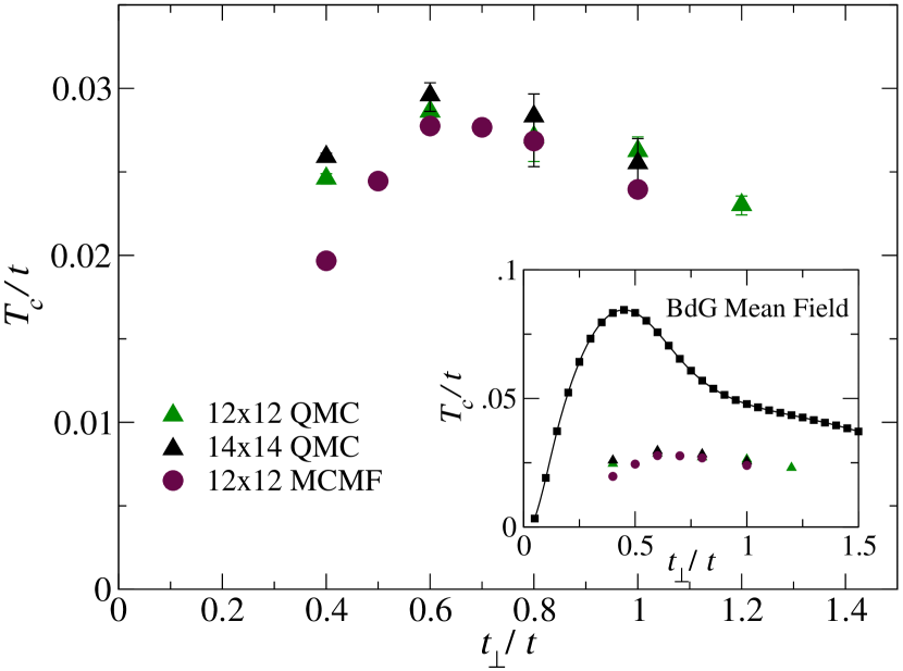
Figure 4: The critical temperature as function of $t_{\perp}$ for a clean bilayer with $U/t=1$ and $n=1.5$, calculated using QMC and MCMF methods. The inset depicts a comparison of these results with the predications of the BdG mean-field theory.

Our results for a clean bilayer with $U/t=1$, total density $n=1.5$ and $L/a=12,14$ appear in Fig. 4. A maximum in $T_{c}$ as function of $t_{\perp}$ is observed at $t_{\perp,{\rm max}}\simeq 0.6t$. While this behavior is akin to the BdG mean-field findings of Ref. Ours, , shown in the inset, the two sets of data differ quantitatively. The peak in $T_{c}$, as calculated by QMC, occurs at somewhat higher values of $t_{\perp}$ and its magnitude, $T_{c,{\rm max}}$, is about 3 times smaller than the corresponding maximum in the BdG mean-field $T_{c}$.

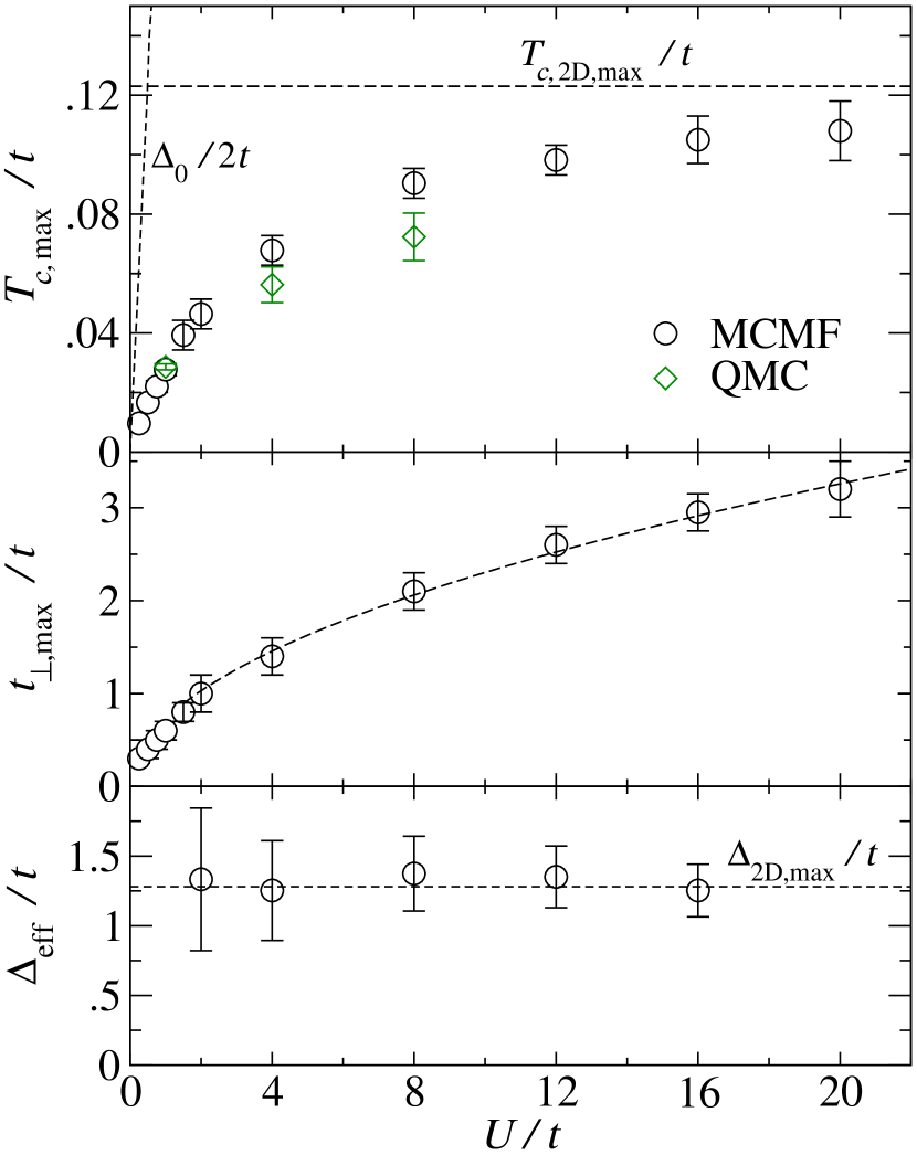
Figure 5: Upper panel: The maximal critical temperature as function of $U/t$ for a clean $12\times 12$ bilayer with $n=1.5$. The horizontal dashed line depicts the highest $T_{c}$ (maximized over $U/t$) of the single-layer attractive Hubbard model with $n=0.5$. The left dashed line corresponds to the mean-field transition temperature of the disconnected Hubbard sites. Middle panel: $t_{\perp,{\rm max}}$ for which $T_{c,{\rm max}}$ is obtained as function of $U/t$. The dashed line is a fit to $t_{\perp,{\rm max}}\propto\sqrt{tU}$. Lower panel: $\Delta_{\rm eff}(t_{\perp,{\rm max}})=t_{\perp,{\rm max}}^{2}/\Delta_{0}$ as function of $U/t$. The dashed line corresponds to the average amplitude of the order parameter at the highest $T_{c}$ of the single-layer attractive Hubbard model with $n=0.5$.

The use of QMC to study the $U/t$ dependence of $T_{c,{\rm max}}$ is restricted by the low temperatures that are encountered in the small $U/t$ regime and the short $\Delta\tau$ required when $U/t$ is large. To partially overcome these difficulties we employ an approximate method which neglects quantum fluctuations of the order parameter. As we saw in Sec. II.3 such an approximation fails for small $t_{\perp}$. However, our findings demonstrate that it is sufficient near the maximal $T_{c}$. In this Monte Carlo Mean Field method (MCMF), (originally introduced by Mayr et al. Mayr in its $d$-wave version), a classical Monte-Carlo scheme is used to average over random configurations of the local pairing field. The partition function is given by

$${\cal Z}=\int\prod_{i=1}^{N}d\Delta_{i}d\Delta_{i}^{*}e^{-(\beta/U)\sum_{i}|\Delta_{i}|^{2}}Z(\{\Delta_{i}\}),$$ (40)

where $Z(\{\Delta_{i}\})$ is the partition function of the BdG quasi-particles for a given configuration of the pairing field. Observables, such as the phase stiffness, are calculated using the quasi-particle Green’s functions and averaged over the pairing field configurations. The critical temperature is determined using Eq. (36), just as in the QMC simulations. As shown in Figs. 4 and 5 MCMF reproduces to within 20% the QMC results for $T_{c,{\rm max}}$ over the range $1\leq U/t\leq 8$ (we attribute the fact that the MCMF $T_{c}$ curve lies below the corresponding QMC curve in the $U/t=1$ system to a different finite size scaling of the two methods). We therefore conclude that the maximal $T_{c}$ is largely governed by thermal fluctuations.

Utilizing the MCMF method to calculate $T_{c,{\rm max}}$ beyond the $U/t$ range which is amenable to QMC simulations one obtains the following behavior, depicted in Fig. 5. First, at small $U/t$ the maximal critical temperature scales with the mean-field temperature, $T_{\rm MF}\approx U/4$, of the disconnected Hubbard sited. The latter is the temperature at which the pairing gap on each site closes and thus sets a maximum conceivable value for $T_{c}$ which takes full advantage of the pairing scale. Numerically, we find for $U<t$ that $T_{c,{\rm max}}\approx T_{\rm MF}/3$. This is to be contrasted with the mean-field result of Ref. Ours, , $T_{c,{\rm max}}\rightarrow T_{\rm MF}$ in the same range of parameters. Presumably, the difference stems from the absence of (predominantly classical) phase fluctuations in the mean-field calculation.

At large $U/t$, $T_{c,{\rm max}}$ seems to saturate to a limiting value, which is close to the maximal $T_{c}$ of the quarter filled two-dimensional attractive Hubbard model.Tcmax-comm Our MCMF results indicate that amplitude fluctuations of the order parameter play a minor role at the $T_{c}$ maximum of both models, changing it by about 5%. We would therefore attempt to understand the above behavior from the perspective of thermal phase fluctuations only. To this end we decouple the interaction term in the original action (1) and integrate out the pairing sites while allowing only spatial phase fluctuation in the pairing field, i.e. assuming $\Delta_{i}(\tau)=\Delta_{0}e^{i\theta_{i}}$. The result is

$$S = -\beta\sum_{i,j,\sigma}\sum_{\omega_{n}}c_{i\sigma}^{\dagger}(\omega_{n})\left[{\cal G}_{ij}^{-1}(\omega_{n})+\frac{t_{\perp}^{2}(i\omega_{n}-\mu)\delta_{ij}}{\omega_{n}^{2}+\mu^{2}+\Delta_{0}^{2}}\right]$$ (41)

$$\times c_{j\sigma}(\omega_{n})+\beta\Delta_{\rm eff}\sum_{i}\sum_{\omega_{n}}\frac{\Delta_{0}^{2}}{\omega_{n}^{2}+\mu^{2}+\Delta_{0}^{2}}$$

$$\times \left[e^{i\theta_{i}}c_{i\uparrow}^{\dagger}(\omega_{n})c_{i\downarrow}^{\dagger}(-\omega_{n})+{\rm H.c.}\right],$$

where

$$\Delta_{\rm eff}=\frac{t_{\perp}^{2}}{\Delta_{0}}.$$ (42)

As shown in Fig. 5, $t_{\perp,{\rm max}}$ scales as $\sqrt{tU}$ for $U>t$. Since $\Delta_{0}\approx U/2$ this implies that at $t_{\perp,{\rm max}}$ and for $U\gg t$ the ${\cal O}(t_{\perp}^{2})$ correction to the first term in the action (41) can be neglected in comparison to ${\cal G}_{ij}^{-1}$. Moreover, since the important contribution to the action comes from frequencies within the metallic bandwidth the prefactor inside the second term of Eq. (41) can be replaced in the limit $U\gg t$ by 1. Within these approximations Eq. (41) becomes the action of a two-dimensional attractive Hubbard whose filling is set by the filling of the metallic layer and whose pairing field amplitude is given by $\Delta_{\rm eff}$. The lower panel of Fig. 5 demonstrates that in the $U>t$ regime $\Delta_{\rm eff}(t_{\perp,{\rm max}})$ coincides with the order parameter amplitude of the two-dimensional attractive Hubbard model at its maximum $T_{c}$ (as obtained using MCMF). In other words, for large $U$ the bilayer achieves its optimal $T_{c}$ by adjusting the inter-layer tunneling $t_{\perp}$ to a point that maps the bilayer onto a single layer attractive Hubbard with an optimal $U/t$ ratio. Since the average pairing amplitude of the latter is of order $t$ Eq. (42) implies the $t_{\perp,{\rm max}}\sim\sqrt{tU}$ scaling mentioned above.

Finally, in order to obtain a rough idea of the effect of disorder on $T_{c,{\rm max}}$ we resort to the mean-field treatment of Ref. Ours, . We apply it to a bilayer with $U=t$ where in the absence of disorder it differs from the QMC and MCMF results by a factor of 3, see Fig. 4. The mean-field approximation consists of decoupling the interaction term $-Uf^{\dagger}_{i\uparrow}f_{i\uparrow}f^{\dagger}_{i\downarrow}f_{i\downarrow}\rightarrow-\Delta^{*}_{i}f_{i\uparrow}f_{i\downarrow}-\Delta_{i}f^{\dagger}_{i\downarrow}f^{\dagger}_{i\uparrow}$, and solving the BdG equations for the disordered bilayer at finite temperature. This is done under the self-consistent condition $\Delta_{i}=U\langle f_{i\uparrow}f_{i\downarrow}\rangle$ and with a phase twist in the $x$ direction, which enters the kinetic part of the Hamiltonian according to

$$-t\sum_{\langle i,j\rangle,\sigma}c^{\dagger}_{i\sigma}c_{j\sigma}\rightarrow-t\sum_{\langle i,j\rangle,\sigma}e^{q_{x}(x_{i}-x_{j})/2a}c^{\dagger}_{i\sigma}c_{j\sigma}.$$ (43)

The free energy, $F$, calculated from the BdG solutions, is then used to evaluate the bare phase stiffness $\rho_{s}^{0}(T)=(a/L)^{2}\partial^{2}F/\partial q_{x}^{2}$, which includes the physics of thermally excited quasiparticles but ignores the renormalization of the stiffness by phase fluctuations.

Figure 6 depicts the estimated maximal critical temperature obtained from the approximate BKT criterion ${\widetilde{T}}_{c,{\rm max}}=(\pi/2)\rho_{s}^{0}({\widetilde{T}}_{c,{\rm max}},t_{\perp,{\rm max}})$ for a bilayer with $L=10a$, and $n=1.5$. The results were averaged over up to 200 realizations of disorder in which every $V_{i}$ was drawn independently from a uniform distribution in the range $[-V,V]$. As shown, the disorder has little effect on $T_{c,{\rm max}}$ as long as it is smaller than the metallic hopping amplitude. For $V/t\gtrsim 2.5$ we found that the system’s dimensionless conductance, $g$, obeys $g<1$, indicating that strong localization effects become important in this range. Such effects enhance phase fluctuations and are expected to induce a transition to an insulating phase, which is not seen in the small system considered by us. We also found that the value of $t_{\perp,{\rm max}}$ is not affected by the disorder and remains fixed at $t_{\perp,{\rm max}}\approx 0.48t$.

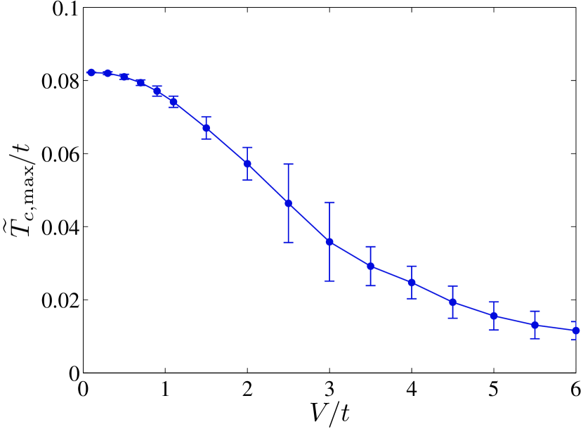
Figure 6: The estimated maximal critical temperature ${\widetilde{T}}_{c,{\rm max}}$ deduced from the approximated BKT criterion ${\widetilde{T}}_{c,{\rm max}}=(\pi/2)\rho_{s}^{0}({\widetilde{T}}_{c,{\rm max}})$ as function of the disorder strength $V$ for $U/t=1$ and $n=1.5$. The bars depict the standard deviation of the distribution of ${\widetilde{T}}_{c,{\rm max}}$. Based on our results for the clean system we expect the actual maximal $T_{c}$ to be about 3 times smaller than the values presented here. For $V/t\gtrsim 2$ strong localization effects likely cause $T_{c}$ to drop even faster and to eventually vanish at a critical disorder strength.

IV Conclusion

Superconductivity contains within itself a built-in tension between its two essential prerequisites: pairing and phase coherence. In all known examples where interactions are strong such that they lead to a large pairing scale a concomitant suppression of the superfluid stiffness, and with it of $T_{c}$, takes place. Canonical examples are the strong interaction regime of the attractive Hubbard model and the underdoped cuprate superconductors. It was suggested that a possible way out of the dilemma is to separate the pairing medium from the conduction electrons, thus maintaining their large phase stiffness.StevePhysica This strategy was pursued in Ref. Ours, and its qualitative feasibility was demonstrated. However, the consequences of superconducting phase fluctuations on the induced stiffness at the interface between the two subsystems were not considered.

In the present work we have shown that phase fluctuations lead to an exponential suppression of the superfluid stiffness when the interlayer coupling is small. For intermediate coupling these fluctuations cause a reduction of $T_{c}$ by factor 3 relative to its value based solely on thermal excitation of quasiparticles. We believe that our results have broader implications beyond the specific model studied here, as they point to the fact that renormalization of the stiffness by phase fluctuations is important in systems with long range phase couplings.

Despite the renormalization, long phase couplings are preferable to short ones from the perspective of increasing $T_{c}$ at the surface of a phase fluctuating superconductor. As we showed, when a metal is overgrown on the surface of a superconductor, additional phase couplings between sites on the interface are established up to distances of the order of the metallic thermal length. This is true whether the added metal forms a two-dimensional layer or is thicker than the thermal length and can therefore be considered as three dimensional. However, within this range the decay of the coupling, technically described by the cooperon, follows $r^{-d}$ in the $d$-dimensional case. This is a result of the fact that in three dimensions the electrons that mediate the coupling spend part of their time moving in the direction perpendicular to the surface, thereby lowering their probability to reach longer distances along the surface within the allotted coherence time $1/T$. Consequently, our analysis suggests that one should attempt to make the metallic layer as thin as possible in order to maximize the induced phase couplings and with them $T_{c}$.

Our results show that disorder has little effect on $T_{c}$, as long as it is weak enough not to cause strong localization. From a practical point of view, a particular form of disorder, namely interface roughness, may actually benefit the enhancement of $T_{c}$.Goren This statement stems from the fact that when the pairing scale is of the order of the metallic bandwidth maximal enhancement occurs at values of the interlayer tunneling which are comparable to the metallic hopping amplitude. Such strong tunneling across the interface may be difficult to achieve. An example can be found in the cuprate bilayersYuli ; Gozar where the intrinsic in-plane hopping is much stronger than the inter-plane one. Nevertheless, if the interface is not perfect so that the pairing medium and the metal locally interpenetrate each other electrons may tunnel between the two laterally, exploiting the large hopping amplitude in this direction.

Appendix A Derivation of the phase action

Here we provide details concerning the derivation of the phase action, Eq. (4). As discussed in Section II.2 we assume that the superconducting amplitude is fixed at its zero temperature value $|\Delta_{i}(\tau)|=\Delta_{0}$ and proceed to write Eqs. (2,II.2) in frequency space. In terms of $\Psi_{i}^{\dagger}(\omega_{m})=[f_{i\uparrow}^{\dagger}(\omega_{m}),f_{i\downarrow}(-\omega_{m})]$ they become

$$S=\sum_{i,j}\sum_{\omega_{m},\omega_{n}}\Psi^{\dagger}_{i}(\omega_{m})\left[M^{(0)}+V^{(0)}+V^{(1)}\right]\Psi_{j}(\omega_{n}),$$ (44)

where

$$M^{(0)}_{ij}(\omega_{m},\omega_{n})=\beta[-i\omega_{m}{\bf I}-\mu\mbox{\boldmath$\sigma$}_{3}+\Delta_{0}\mbox{\boldmath$\sigma$}_{1}]\delta_{ij}\delta_{\omega_{m},\omega_{n}},$$

$$V^{(0)}_{ij}(\omega_{m},\omega_{n})=\frac{\beta}{2}(\omega_{m}-\omega_{n})\theta_{i}(\omega_{m}-\omega_{n})\mbox{\boldmath$\sigma$}_{3}\delta_{ij}\delta_{\omega_{m},\omega_{n}},$$

$$V^{(1)}_{ij}(\omega_{m},\omega_{n})=\frac{\beta}{2}t_{\perp}^{2}\sum_{\Omega_{n}}\left[({\bf I}+\mbox{\boldmath$\sigma$}_{3}){\cal G}_{ij}(\omega_{m}-\Omega_{n})F_{i}(\Omega_{n})\right.$$

$$\times F_{j}^{*}(\Omega_{n}+\omega_{n}-\omega_{m})-({\bf I}-\mbox{\boldmath$\sigma$}_{3}){\cal G}_{ji}(-\omega_{n}-\Omega_{n})F_{j}(\Omega_{n})$$

$$\left.\times F_{i}^{*}(\Omega_{n}+\omega_{n}-\omega_{m})\right].$$ (45)

Here, and throughout, $\omega_{n}$ and $\Omega_{n}$ are fermionic and bosonic Matsubara frequencies, respectively. We also denoted

$$F_{i}(\tau)=e^{-i\theta_{i}(\tau)/2}=\sum_{\Omega_{n}}F_{i}(\Omega_{n})e^{-i\Omega_{n}\tau}.$$ (46)

Our goal is to integrate out the fermions to obtain

$$S_{\theta} = -{\rm Tr}\ln[M^{(0)}+V^{(0)}+V^{(1)}]$$ (47)

$$\approx -{\rm Tr}\ln[M^{(0)}]-{\rm Tr}\left\{{M^{(0)}}^{-1}[V^{(0)}+V^{(1)}]\right\}$$

$$+\frac{1}{2}{\rm Tr}\left\{{M^{(0)}}^{-1}[V^{(0)}+V^{(1)}]\right\}^{2}.$$

$M^{(0)}$ is independent of $\theta$ and thus plays no role here. It is also trivial to see that the linear term in $V^{(0)}$ vanishes. Hence, we turn our attention to

$$-{\rm Tr}\left[{M^{(0)}}^{-1}V^{(1)}\right]$$

$$\approx{\rm min}\left(1,\frac{8t}{\Delta_{0}}\right)\frac{t_{\perp}^{2}N_{F}a^{2}}{T\Delta_{0}^{2}}\sum_{i,\Omega_{n}}\Omega_{n}^{2}|\theta_{i}(\Omega_{n})|^{2},$$ (48)

evaluated for $\Omega_{n}<\Delta_{0}$. This, however, is negligible compared to

$$\frac{1}{2}{\rm Tr}\left[{M^{(0)}}^{-1}V^{(0)}{M^{(0)}}^{-1}V^{(0)}\right]$$

$$=\frac{1}{8T\Delta_{0}}\sum_{i,\Omega_{n}}\Omega_{n}^{2}|\theta_{i}(\Omega_{n})|^{2}+{\cal O}\left(\frac{\mu^{2}\Omega_{n}^{2}+\Omega_{n}^{4}}{T\Delta_{0}^{3}}\right),$$ (49)

which constitutes the first term in Eq. (4).

The term $\frac{1}{2}{\rm Tr}\left[{M^{(0)}}^{-1}V^{(1)}{M^{(0)}}^{-1}V^{(1)}\right]$ contains two contributions. The first is

$$\!\!\!\!\!C_{1}=-\sum_{i,j}\sum_{\Omega_{m},\Omega_{n}}\sum_{\omega_{m},\omega_{n}}\frac{t_{\perp}^{4}\Delta_{0}^{2}}{(\omega_{m}^{2}+\mu^{2}+\Delta_{0}^{2})(\omega_{n}^{2}+\mu^{2}+\Delta_{0}^{2})}$$

$$\;\;\times\;F_{i}(\Omega_{n})F_{j}^{*}(\Omega_{n}+\omega_{m}-\omega_{n}){\cal G}_{ij}(-\omega_{m}-\Omega_{n})$$

$$\;\;\times\;F_{i}(\Omega_{m})F_{j}^{*}(\Omega_{m}+\omega_{n}-\omega_{m}){\cal G}_{ij}(\omega_{m}-\Omega_{m}).$$ (50)

Its evaluation requires the disorder average $P_{ij}(\omega_{n},\Omega_{n})=\left\langle{\cal G}_{ij}\left(\omega_{n}\right){\cal G}_{ij}\left(\omega_{n}+\Omega_{n}\right)\right\rangle$. The metallic layer is assumed to contain Gaussian disorder obeying $\langle V_{i}\rangle=0$ and $\langle V_{i}V_{j}\rangle=n{\cal V}^{2}\delta_{ij}$, where $n$ is the average number of impurities per site and ${\cal V}^{2}=\langle V_{i}^{2}\rangle/n$. The disorder scattering is characterized by the elastic mean free time $\tau_{e}=[2\pi N_{F}a^{2}n{\cal V}^{2}]^{-1}$ and is assumed weak, $k_{F}l_{e}\gg 1$. The leading contribution to the above average comes from the cooperon, i.e. , the sum of ladder diagrams whose legs are constructed from disorder-averaged Green’s functions and whose rungs are disorder lines. In momentum space the cooperon takes the formAkkermans

$$P({\bf Q},\omega_{n},\Omega_{n}) = \frac{P_{0}({\bf Q},\omega_{n},\Omega_{n})}{1-(2\pi N_{F}a^{2}\tau_{e})^{-1}P_{0}({\bf Q},\omega_{n},\Omega_{n})}.$$

Here

$$P_{0}({\bf Q},\omega_{n},\Omega_{n})=\frac{1}{N}\sum_{{\bf K}}\frac{1}{-i\omega_{n}-\xi_{{\bf k}}-\frac{i}{2\tau_{e}}{\rm sign}(\omega_{n})}$$

$$\times\frac{1}{i(\omega_{n}+\Omega_{n})-\xi_{{\bf k}+{\bf Q}}+\frac{i}{2\tau_{e}}{\rm sign}(\omega_{n}+\Omega_{n})},$$ (52)

with $\xi_{{\bf k}}=-2t[\cos(k_{x}a)+\cos(k_{y}a)]+\epsilon-\mu$, reduces to the cooperon of the clean system in the limit $\tau_{e}\rightarrow\infty$. For $Q=|{\bf Q}|\ll k_{F}$ it becomes

$$P_{0}({\bf Q},\omega_{n},\Omega_{n})=\pi N_{F}a^{2}\tau_{e}\frac{\left|{\rm sign}(\omega_{n}+\Omega_{n})-{\rm sign}(\omega_{n})\right|}{\sqrt{(1+|\Omega_{n}|\tau_{e})^{2}+(Ql_{e})^{2}}}.$$ (53)

For a diffusive system, and as long as $Ql_{e}\ll 1$ and $|\omega_{n}|\tau_{e}\ll 1$, one may expand the square root in Eq. (53), and plug the result into Eq. (A) to find

$$P({\bf Q},\omega_{n},\Omega_{n})=\pi N_{F}a^{2}\frac{\left|{\rm sign}(\omega_{n}+\Omega_{n})-{\rm sign}(\omega_{n})\right|}{|\Omega_{n}|+DQ^{2}},$$ (54)

where $D=l_{e}^{2}/(2\tau_{e})$ is the diffusion constant. At this point we would like to note that an additional time scale, the phase breaking time $\tau_{\varphi}$, can be phenomenologically introduced into the problem and act as a mass term for the cooperon. It is knownAAK that interactions in two dimensions lead to $\tau_{\varphi}^{-1}\sim(T\ln g)/g$, where $g$ is the dimensionless conductance of the disordered layer. Our treatment of the disorder is valid for $g\gg 1$ and therefore $\tau_{\varphi}^{-1}\ll T$. Consequently, it does not alter our results and is not considered further.

Transforming back to real space leads in the clean limit and $r_{ij}\gg k_{F}^{-1}$ to

$$P_{ij}(\omega_{n},\Omega_{n}) = \frac{1}{2}N_{F}a^{4}\left|{\rm sign}(\omega_{n}+\Omega_{n})-{\rm sign}(\omega_{n})\right|$$ (55)

$$\times \frac{1}{v_{F}r_{ij}}e^{-|\Omega_{m}|r_{ij}/v_{F}},$$

while for the diffusive system and $r_{ij}\gg l_{e}$ the result is

$$P_{ij}(\omega_{n},\Omega_{n}) = \frac{N_{F}a^{4}}{2D}\left|{\rm sign}(\omega_{n}+\Omega_{n})-{\rm sign}(\omega_{n})\right|$$ (56)

$$\times K_{0}\left(r\sqrt{\frac{|\Omega_{n}|}{D}}\right),$$

where $K_{0}(x)$ is the Bessel function of the first kind.

Plugging Eq. (55) into Eq. (A), defining $\omega=\Omega_{m}-\omega_{m}$, $\omega^{\prime}=\Omega_{n}+\omega_{m}$ and carrying out the summation over $\omega_{m}$ and $\omega_{n}$ using the fact that at the relevant low temperature range they can be approximated by integrals one obtains $C_{1}=\sum_{i,j}C_{1,ij}$, where in the clean limit

$$C_{1,ij}=-\frac{t_{\perp}^{4}N_{F}a^{4}T^{2}}{8v_{F}r_{ij}}\int_{0}^{\beta}\!\prod_{n=1}^{4}d\tau_{n}e^{-\Delta_{0}|\tau_{1}-\tau_{2}|}e^{-\Delta_{0}|\tau_{3}-\tau_{4}|}$$

$$\,\times\;F_{i}(\tau_{1})F_{i}(\tau_{2})F_{j}^{*}(\tau_{3})F_{j}^{*}(\tau_{4})\sum_{\omega,\omega^{\prime}}\left|{\rm sign}(\omega^{\prime})-{\rm sign}(\omega)\right|$$

$$\,\times\;e^{i[\omega(\tau_{1}-\tau_{3})+\omega^{\prime}(\tau_{2}-\tau_{4})]-|\omega^{\prime}-\omega|r_{ij}/v_{F}}.$$ (57)

For $r_{ij}>l_{T}=v_{F}/T$ the sum is dominated by the lowest frequency difference and $C_{1,ij}$ decays as $(1/r_{ij})e^{-2\pi r_{ij}/l_{T}}$. For $r_{ij}\ll l_{T}$ the sums may be approximated by integrals with the result

$$C_{1,ij}=-\frac{t_{\perp}^{4}N_{F}a^{4}}{8\pi^{2}v_{F}r_{ij}}\int_{0}^{\beta}\!\prod_{n=1}^{4}d\tau_{n}e^{-\Delta_{0}|\tau_{1}-\tau_{2}|}e^{-\Delta_{0}|\tau_{3}-\tau_{4}|}$$

$$\hskip 11.38092pt\times\;\frac{(\tau_{1}-\tau_{3})(\tau_{2}-\tau_{4})+(\frac{r_{ij}}{v_{F}})^{2}}{[(\tau_{1}-\tau_{3})^{2}+(\frac{r_{ij}}{v_{F}})^{2}][(\tau_{2}-\tau_{4})^{2}+(\frac{r_{ij}}{v_{F}})^{2}]}$$

$$\hskip 11.38092pt\times\;F_{i}(\tau_{1})F_{i}(\tau_{2})F_{j}^{*}(\tau_{3})F_{j}^{*}(\tau_{4}).$$ (58)

Owing to Eq. (A) $\langle F_{i}(\tau)F_{i}^{*}(\tau^{\prime})\rangle=e^{-\Delta_{0}|\tau-\tau^{\prime}|/2}$, which means that $F_{i}$ may be considered constant within a time window of order $\Delta_{0}^{-1}$. This fact and the exponential factors in Eq. (A) enable us to approximate $F_{i}(\tau_{1})=F_{i}(\tau_{2})$ and $F_{j}^{*}(\tau_{3})=F_{j}^{*}(\tau_{4})$, leading to the coupling $\cos[\theta_{i}(\tau)-\theta_{j}(\tau^{\prime})]$ mediated by pair tunneling between the two sites, and constituting the second term in the action, Eq. (4). The associated kernel may be evaluated in the range $a\ll r_{ij}\ll\xi=v_{F}/\Delta_{0}$ by taking $r_{ij}\rightarrow 0$ in Eq. (A) and carrying out the integration over $\tau_{2}$ and $\tau_{3}$. The result

$$K(r,\tau)=\frac{t_{\perp}^{4}N_{F}a^{4}}{8\pi^{2}v_{F}r}\left[\left(e^{\Delta_{0}\tau}{\rm Ei}[-\Delta_{0}\tau]-e^{-\Delta_{0}\tau}{\rm Ei}[\Delta_{0}\tau]\right)^{2}\right.$$

$$\hskip 22.47748pt+\left.\pi^{2}e^{-2\Delta_{0}|\tau|}\right],$$ (59)

where ${\rm Ei}(x)$ is the exponential integral function, is approximated by Eq. (6). For $l_{T}\gg r_{ij}\gg\xi$ we may expand the integrand in Eq. (A) to second order in $\tau_{1}-\tau_{2}$ and $\tau_{3}-\tau_{4}$. Integration over $\tau_{2}$ and $\tau_{3}$ then yields Eq. (5).

Repeating the derivation using Eq. (56) for the diffusive case produces a similar coupling with the kernel

$$K(r,\tau) = \frac{t_{\perp}^{4}\Delta_{0}N_{F}a^{4}T}{\pi D}\sum_{\omega>0}\frac{1}{\omega(\omega^{2}+\Delta_{0}^{2})}K_{0}\left(r\sqrt{\frac{2\omega}{D}}\right)$$ (60)

$$\times \int_{-\infty}^{\infty}d\eta e^{-2\Delta_{0}|\eta|}\frac{\sin[2\omega(\tau+\eta)]}{\tau+\eta}$$

$$\times \left[\omega\cos(2\omega\eta)+\Delta_{0}\sin(2\omega|\eta|)\right].$$

The exponential decay of $K_{0}(x)$ for $x>1$ induces the decay of the kernel when $r_{ij}>l_{T}=\sqrt{D/T}$. This also means that for $l_{T}\gg r_{ij}\gg\xi=\sqrt{D/\Delta_{0}}$ only $\omega<\Delta_{0}(\xi/r)^{2}$ contribute. Since the exponential factor in Eq. (60) implies $|\eta|<\Delta_{0}$ we may expand the integrand in $\omega|\eta|<1$ and evaluate the integrals with the approximated result Eq. (7).

The second contribution to the effective action coming from $\frac{1}{2}{\rm Tr}\left[{M^{(0)}}^{-1}V^{(1)}{M^{(0)}}^{-1}V^{(1)}\right]$ is

$$\!\!\!\!\!\!\!\!\!\!\!\!C_{2}=\sum_{i,j}\sum_{\Omega_{m},\Omega_{n}}\sum_{\omega_{m},\omega_{n}}\frac{t_{\perp}^{4}(i\omega_{m}+\mu)(i\omega_{n}+\mu)}{(\omega_{m}^{2}+\mu^{2}+\Delta_{0}^{2})(\omega_{n}^{2}+\mu^{2}+\Delta_{0}^{2})}$$

$$\!\!\!\times\;F_{i}(\Omega_{n})F_{j}^{*}(\Omega_{n}+\omega_{m}-\omega_{n}){\cal G}_{ij}(-\omega_{m}-\Omega_{n})$$

$$\!\!\!\times\;F_{j}(\Omega_{m})F_{i}^{*}(\Omega_{m}+\omega_{n}-\omega_{m}){\cal G}_{ji}(-\omega_{n}-\Omega_{m}).$$ (61)

Following a similar line of derivation to the one taken above we find that this contribution corresponds to a coupling $\cos\left\{\frac{1}{2}[\theta_{i}(\tau)-\theta_{j}(\tau)-\theta_{i}(\tau^{\prime})+\theta_{j}(\tau^{\prime})]\right\}$, induced by single-particle tunneling between the sites.schonreview However, we find that it has a negligible effect in comparison to the pair-tunneling term. For example in the clean system and for $l_{T}\gg r_{ij}\gg\xi$ the associated kernel reads

$${\tilde{K}}(r,\tau)=\frac{t_{\perp}^{4}N_{F}a^{4}\mu^{2}}{2\pi^{2}\Delta_{0}^{4}v_{F}}\frac{1}{r}\frac{\tau^{2}-(r/v_{F})^{2}}{[\tau^{2}+(r/v_{F})^{2}]^{2}}.$$ (62)

Applying the mean field treatment of Sec. II.4 to this term yields an average coupling constant ${\bar{g}}\simeq(2t_{\perp}^{4}N_{F}a^{2}\mu^{2})/(N_{\rm rod}\pi\Delta_{0}^{5})$ to be compared with ${\bar{g}}=(t_{\perp}^{4}N_{F}a^{2}/N_{\rm rod}\Delta_{0}^{3})\ln(l_{T}/\xi)$, Eq. (33).

Finally, the ${\rm Tr}\left[{M^{(0)}}^{-1}V^{(0)}{M^{(0)}}^{-1}V^{(1)}\right]$ piece in Eq. (47) can be shown to result in a $(\partial_{\tau}\theta_{i})^{2}$ term, which is of order $t_{\perp}^{2}$ and is therefore insignificant compared to Eq. (A).

References

- (1) E. Berg, D. Orgad, and S. A. Kivelson, Phys. Rev. B 78, 094509 (2008).
- (2) S. Okamoto S and T. A. Maier, Phys. Rev. Lett. 101, 156401 (2008).
- (3) L. Goren and E. Altman, Phys. Rev. B 79, 174509 (2009).
- (4) O. Yuli, I. Asulin, O. Millo, D. Orgad, L. Iomin, and G. Koren, Phys. Rev. Lett. 101, 057005 (2008); G. Koren and O. Millo, Phys. Rev. B 81, 134516 (2010).
- (5) A. Gozar, G. Logvenov, L. .F. Kourkoutis, A. T. Bollinger, L. A. Giannuzzi, D. A. Muller, and I. Bozovic, Nature (London) 455, 782 (2008).
- (6) P. W. Anderson, J. Phys. Chem. Solids 11, 26 (1959).
- (7) M. Ma, B. I. Halperin, and P. A. Lee, Phys. Rev. B 34, 3136 (1986).
- (8) M. P. A. Fisher, Phys. Rev. Lett. 57, 885 (1986).
- (9) S. Chakravarty, G.-L. Ingold, S. Kivelson, and G. Zimanyi, Phys. Rev. B 37, 3283 (1988).
- (10) A. Ghosal, M. Randeria, and N. Trivedi, Phys. Rev. Lett. 81, 3940 (1998).
- (11) I. S. Beloborodov, K. B. Efetov, A. V. Lopatin, and V. M. Vinokur, Phys. Rev. B 71, 184501 (2005).
- (12) Y. Dubi, Y. Meir, Y. Avishai, Nature (London) 449, 876 (2007).
- (13) B. Spivak, P. Oreto, and S. A. Kivelson, Phys. Rev. B 77, 214523 (2008).
- (14) T. Paiva, R. R. dos Santos, R. T. Scalettar, and P. J. H. Denteneer, Phys. Rev. B 69, 184501 (2004).
- (15) M. Hasenbusch. J. Phys. A 38, 5869 (2005).
- (16) U. Wolff, Phys. Rev. Lett. 62, 361 (1989).
- (17) M. Antoni and S. Ruffo, Phys. Rev. E 52, 2361 (1995).
- (18) B. Halperin and D. Nelson, J. Low Temp. Phys. 36, 599 (1979).
- (19) R. T. Scalettar, N. Trivedi, and C. Huscroft, Phys. Rev. B 59, 4364 (1999).
- (20) S. De Palo, C. Castellani, C. Di Castro, and B. K. Chakraverty, Phys. Rev. B 60, 564 (1999).
- (21) L. Benfatto, A. Toschi, and S. Caprara, Phys. Rev. B 69, 184510 (2004).
- (22) D. J. Scalapino, S. R. White, and S. Zhang, Phys. Rev. B 47, 7995 (1993).
- (23) R. Blankenbecler, D. J. Scalapino, and R. L. Sugar, Phys. Rev. D 24, 2278 (1981).
- (24) J. E. Hirsch, Phys. Rev. B 38, 12023 (1988).
- (25) M. Mayr, G. Alvarez, C. Şen, and E. Dagotto, Phys. Rev. Lett. 94, 217001 (2005).
- (26) According to our MCMF results of the quarter-filled two-dimensional attractive Hubbard model occurs at . QMC simulations of an system yield a broad maximum in the range with . These results are to be compared with the findings of R. T. Scalettar, E. Y. Loh, J. E. Gubernatis, A. Moreo, S. R. White, D. J. Scalapino, R. L. Sugar, and E. Dagotto, Phys. Rev. Lett. 62, 1407 (1989), and of A. Moreo and D. J. Scalapino, Phys. Rev. Lett. 66, 946 (1991), who reported a maximum at . Note, however, that their conclusion was based on the magnitude of the pairing correlations and not on the phase stiffness, see also Ref. Paiva04, .
- (27) S. A. Kivelson, Physica B 318, 61 (2002).
- (28) L. Goren and E. Altman, Phys. Rev. B 84, 094508 (2011).
- (29) E. Akkermans and G. Montambaux, Mesoscopic Physics of Electrons and Photons, (Cambridge University Press, 2007).
- (30) B. L. Altshuler, A. G. Aronov, and D. E. Khmelnitsky, J. Phys. C 15, 7367 (1982).
- (31) G. Schn and A. D. Zaikin, Phys. Rep. 198, 237 (1990).