The exponential map at a cuspidal singularity

Abstract.

We study spaces with a cuspidal (or horn-like) singularity embedded in a smooth Riemannian manifold and analyze the geodesics in these spaces which start at the singularity. This provides a basis for understanding the intrinsic geometry of such spaces near the singularity. We show that these geodesics combine to naturally define an exponential map based at the singularity, but that the behavior of this map can deviate strongly from the behavior of the exponential map based at a smooth point or at a conical singularity: While it is always surjective near the singularity, it may be discontinuous and non-injective on any neighborhood of the singularity. The precise behavior of the exponential map is determined by a function on the link of the singularity which is an invariant of the induced metric. Our methods are based on the Hamiltonian system of geodesic differential equations and on techniques of singular analysis. The results are proved in the more general natural setting of manifolds with boundary carrying a so-called cuspidal metric.

1. Introduction

Geodesics are among the fundamental objects of differential geometry. On a smooth Riemannian manifold the geodesics starting at a point $p$ are classified by and smoothly depend on their initial velocity vector, and combine to define the exponential map based at $p$, which in turn yields normal coordinates and important geometric information about the manifold. Also, geodesics arise in the study of the propagation of waves on the manifold as paths along which singularities of solutions of the linear wave equation travel.

Much less is known about the behavior of geodesics on singular spaces. Here by a geodesic we always mean a locally shortest curve. Our general aim is to analyze the full local asymptotic behavior of the family of geodesics reaching, or starting at, a singularity. Previously, Bernig and Lytchak [BeLy] obtained first order information for geodesics on general real algebraic sets $X\subset\mathbb{R}^{n}$, by showing that any geodesic reaching a singular point $p$ of $X$ in finite time must have a limit direction at $p$. In the special situation of isolated conical singularities $p$, Melrose and Wunsch [MeWu] obtain full asymptotic information by showing that the geodesics starting at $p$ define a smooth foliation of a neighborhood of $p$ and thus may be combined to define a smooth exponential map based at $p$, analogous to Theorem 1.2 below.

In this paper we analyze the family of geodesics starting at an isolated cuspidal singularity, defined below. Our method is based on the geodesic differential equations and yields full asymptotic information about the geodesics. We will see that there is a much richer range of possible local behavior than in the case of conical singularities; for example, there is a natural notion of exponential map based at the singularity, but this map may be non-injective or discontinuous on any neighborhood of the singularity.

A natural setting for our investigation is the notion of cuspidal manifold. This is a smooth (that is, $C^{\infty}$) manifold, $M$, with compact boundary, equipped with a semi-Riemannian metric, ${\bf g}$, which is Riemannian in the interior $\mathring{M}$ and in a neighborhood $U$ of the boundary $\partial M$ can be written

(1) $${\bf g}_{|U}=\left(1-k(k-1)r^{2k-2}S+O(r^{2k-1})\right)\,dr^{2}+r^{2k}h\,.$$

Here $r$ is a boundary defining function for $M$ (that is, $r\in C^{\infty}(M)$ is positive in $\mathring{M}$, vanishes on $\partial M$ and satisfies $dr_{{\bf p}}\neq 0$ for all ${\bf p}\in\partial M$), $S$ is a smooth function on $\partial M$ and $h$ is a smooth symmetric two-tensor on $U$ whose restriction to $\partial M$, denoted ${\bf g}_{\partial M}$, is positive definite. Finally,

$$k\geq 2\text{ is an integer, called the {\em order} of the cuspidal manifold.}$$

At first reading it may be useful to think of $k=2$, so that ${\bf g}_{|U}=(1-2r^{2}S+O(r^{3}))\,dr^{2}+r^{4}h$. In fact, it follows from our results that cusps of different orders behave qualitatively the same with respect to the questions we investigate.

We call ${\bf g}$ a cuspidal metric of order $k$. A given cuspidal metric defines invariantly the quantities

$$S\in C^{\infty}(\partial M)\quad\text{and}\quad{\bf g}_{\partial M},\text{ a Riemannian metric on }\partial M$$

(more precisely, $S$ is only determined up to addition of a locally constant function) and fixes $r$ to order $2k-1$. For simplicity we will fix a boundary defining function $r$ throughout.

Cuspidal manifolds of order $k$ arise as resolutions of spaces $X$ with isolated cuspidal singularity $p\in X$ or order $k$. These are subsets $X\subset\mathbb{R}^{n}$ so that $X\setminus p$ is a submanifold of $\mathbb{R}^{n}$ and so that $X$ is given by the following local model in a neighborhood $U^{\prime}$ of $p$: Let $p=0$. Then, with $\mathbb{R}_{+}=[0,\infty)$,

(2) $$X\cap U^{\prime}=\beta({\widetilde{X}}),\quad\beta:\mathbb{R}^{n-1}\times\mathbb{R}_{+}\to\mathbb{R}^{n},\quad(u,z)\mapsto(z^{k}u,z)$$

where ${\widetilde{X}}\subset\mathbb{R}^{n-1}\times\mathbb{R}_{+}$ is a smooth manifold with compact boundary, which satisfies

(2’) $$\partial{\widetilde{X}}\subset E:=\mathbb{R}^{n-1}\times\{0\},\quad{\widetilde{X}}\text{ intersects $E$ transversally.}$$

We call ${\widetilde{X}}$ a resolution of $X$. See Figure 1.

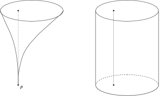
Figure 1. A cuspidal surface singularity $X$ and its resolution ${\widetilde{X}}$; the dotted lines are explained in Remark 7.4

Now if $g$ is any smooth Riemannian metric on the ambient space $\mathbb{R}^{n}$ then the restriction of $g$ to the manifold $X\setminus p$ pulls back under $\beta$ to a Riemannian metric on the interior of ${\widetilde{X}}$. We will prove that this metric extends smoothly to the boundary, and that the extension is a cuspidal metric on ${\widetilde{X}}$. In this sense the resolution of a space with cuspidal singularity is a cuspidal manifold $(M,{\bf g})=({\widetilde{X}},\beta^{*}g)$.

Let $(M,{\bf g})$ be a cuspidal manifold. Since ${\bf g}$ is Riemannian over the interior $\mathring{M}$, locally shortest curves in $\mathring{M}$ are precisely the unit speed solutions of the geodesic differential equations. We call these solutions geodesics on $M$. We are interested in those geodesics starting at the boundary, that is, geodesics $\gamma:(T_{-},T_{+})\to\mathring{M}$ for which $\lim_{\tau\to T_{-}}r(\gamma(\tau))=0$. Here $T_{-}\in\mathbb{R}\cup\{-\infty\}$. If $\lim_{\tau\to T_{-}}\gamma(\tau)$ exists then we call it the starting point of $\gamma$.

Our first theorem shows that, under certain assumptions, geodesics starting at the boundary have a starting point on $\partial M$, and characterizes the possible starting points. Recall that a critical point of $S\in C^{\infty}(\partial M)$ is a point ${\bf p}\in\partial M$ where the differential $dS_{|{\bf p}}$ vanishes.

Theorem 1.1.

Let $(M,{\bf g})$ be a cuspidal manifold. Assume that either $S$ is constant or the critical points of $S$ are isolated.

Then there are $r_{0}>0$, $\tau_{0}>0$ so that the following is true: Let $\gamma:(T_{-},T_{+})\to\mathring{M}$ be a maximal geodesic and assume that for some $T\in(T_{-},T_{+})$ the initial part $\gamma_{|(T_{-},T)}$ is contained in $\{r<r_{0}\}$. Then

1. $T_{-}$ is finite and the starting point $\lim_{\tau\to T_{-}}\gamma(\tau)$ exists.

2. The starting point of $\gamma$ lies on $\partial M$ and is a critical point of $S$.

3. $T_{+}-T_{-}\geq\tau_{0}$, i.e. the geodesic exists at least for time $\tau_{0}$.

Also, the following converse to (b) holds: Each critical point of $S$ is the starting point of a geodesic on $M$.

Our next theorem says that for constant $S$ we have a smooth foliation by geodesics of a neighborhood of $p$, analogous to the Theorem of Melrose and Wunsch [MeWu] in the conical case.

Theorem 1.2.

Let $(M,{\bf g})$ be a cuspidal manifold. Assume $S$ is constant. Then to each ${\bf p}\in\partial M$ there is a unique geodesic $\gamma_{\bf p}$ starting at ${\bf p}$ at time $\tau=0$. Furthermore, there is $\tau_{0}>0$ and a neighborhood $U$ of $\partial M$ in $M$ such that the exponential map

$$\exp_{{\partial M}}:\partial M\times[0,\tau_{0})\to U\subset M,\quad({\bf p},\tau)\mapsto\gamma_{\bf p}(\tau)$$

is a diffeomorphism.

See the left picture in Figure 2.

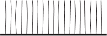
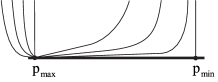
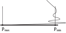
Figure 2. Geodesics in the cases $S=$ const, $S_{\varphi\varphi}<a_{k}$ and $S_{\varphi\varphi}({{\bf p}_{\text{min}}})>a_{k}$. The bold line is ${\partial M}$. The points ${{\bf p}_{\text{max}}}$ and ${{\bf p}_{\text{min}}}$ are a maximum resp. minimum of $S$.

For a general cuspidal manifold, where $S$ need not be constant, it seems clear that a full neighborhood of the boundary is covered by geodesics starting at the boundary, since for any interior point of $M$ any shortest curve from this point to the boundary must be a geodesic. We will not attempt to make this argument precise here (that is, prove existence of a minimizer) but rather analyze the case where $S$ is a Morse function much more precisely, mostly in the case of surfaces.

For our next theorems we assume that $S$ is a Morse function. That is, all critical points are non-degenerate (i.e. the Hessian of $S$ at these points is a non-degenerate quadratic form). This implies that the critical points are isolated.

The behavior of geodesics hitting a non-degenerate critical point ${\bf p}$ of $S$ can be analyzed very precisely in a neighborhood of ${\bf p}$. See for example Proposition 4.2 for the case of local maxima and minima of $S$. We will now focus on surfaces $M$, for which we can analyze how these local pictures fit together in a full neighborhood of $\partial M$. First, we show that there is an exponential map. To simplify the exposition we assume in the following theorems that ${\partial M}$ is connected.

Theorem 1.3.

Let $(M,{\bf g})$ be a cuspidal surface with connected boundary. Assume that $S$ is a Morse function. There is a parametrization $q\mapsto\gamma_{q}$, $q\in{\bf S}^{1}$, of the set of geodesics starting at ${\partial M}$ at time $\tau=0$ so that the map

(3) $$\exp_{{\partial M}}:{\bf S}^{1}\times(0,\tau_{0})\to U\setminus{\partial M},\quad(q,\tau)\mapsto\gamma_{q}(\tau)$$

is defined and surjective for some $\tau_{0}>0$ and some neighborhood $U$ of ${\partial M}$.

The full asymptotic behavior of $\exp_{{\partial M}}$ as $\tau\to 0$ can be described explicitly in terms of $S$.

The parametrization $q\mapsto\gamma_{q}$ is uniquely determined, up to homeomorphisms of ${\bf S}^{1}$, by the requirement that it preserves cyclic ordering in a suitable sense, explained after Definition 6.1. However, $\exp_{{\partial M}}$ need not be a diffeomorphism, it may even be discontinuous. See Section 6 for details.

Whether the exponential map is a homeomorphism onto a neighborhood of the boundary or not is mostly determined by the size of the second derivative of $S$, and the number

(4) $$a_{k}=\frac{(2k-1)^{2}}{2k(k-1)}=2+\frac{1}{2k(k-1)}$$

(for example, $a_{2}=9/4$) turns out to be the determining threshold, where $k$ is the order of the cusp. This is made precise in the next two theorems. Here and throughout we denote by $S_{\varphi}$, $S_{\varphi\varphi}$ the first and second derivatives of $S$ with respect to a coordinate $\varphi$ on $\partial M$.

Theorem 1.4.

Let $(M,{\bf g})$ be a cuspidal surface of order $k$ with connected boundary. Assume that $S$ is a Morse function, that $S_{\varphi\varphi}<a_{k}$ on $\partial M$ and that $S_{\varphi\varphi}$ never takes the value $2$ at any local minimum, where $\varphi$ is an arc length parameter on $\partial M$. Then the exponential map (3) is a homeomorphism for suitable $\tau_{0}$, $U$.

In particular, there is a neighborhood of $\partial M$ such that $U\setminus{\partial M}$ is foliated by geodesics starting at ${\partial M}$.

The exponential map (3) extends to the boundary by letting $\exp_{{\partial M}}(q,0)$ be the starting point of $\gamma_{q}$. However, unlike in the case of constant $S$, the extension ${\bf S}^{1}\times[0,\tau_{0})\to U$ is not continuous in $q$ if $S$ is a Morse function; this is clear since the image of ${\bf S}^{1}\times\{0\}$ is a finite set with at least two elements, a maximum and minimum of $S$.

The value $a_{k}$ in Theorem 1.4 is optimal in the following sense.

Theorem 1.5.

Let $(M,{\bf g})$ be a cuspidal surface of order $k$ with connected boundary. Assume that $S$ is a Morse function and that $S_{\varphi\varphi}>a_{k}$ at some minimum of $S$, for an arc length parameter $\varphi$ on ${\partial M}$. Then the exponential map (3) is not injective for any $\tau_{0}>0$.

That is, in any neighborhood $U$ of ${\partial M}$ there are points through which at least two geodesics starting at the boundary pass.

Theorems 1.4 and 1.5 are illustrated in Figure 2, middle and right.

We also show that the conditions on $S$ in Theorem 1.4 are satisfied if $M$ arises from a cuspidal surface singularity $X$ and if $\partial{\widetilde{X}}$ is contained in the boundary of a strictly convex subset of $\mathbb{R}^{n-1}$ which contains the origin, and is never doubly tangent to a sphere centered at the origin. See Theorem 7.6.

Theorems 1.2, 1.3, 1.4 and 1.5 may be summarized as follows, in the case of surfaces: There is a well-defined exponential map. For constant $S$ it is a smooth diffeomorphism near the boundary. If $S$ is not too far from constant then it is a homeomorphism, though not on the boundary. If $S$ is far from constant then it may be not injective and also discontinuous.

Main ideas, outline of the proofs

To simplify the notation, we assume in this outline that $k=2$. Thus the metric on a neighborhood $U$ of the boundary of $M$ is

(5) $${\bf g}_{|U}=(1-2r^{2}S+O(r^{3}))\,dr^{2}+r^{4}h\,.$$

Let ${\bf g}^{*}$ be the metric on the cotangent bundle $T^{*}\mathring{M}$ dual to ${\bf g}$. Consider the energy function (Hamiltonian) $\widetilde{E}=\frac{1}{2}{\bf g}^{*}$ and the associated Hamiltonian vector field $\widetilde{{\bf W}}$ on $T^{*}\mathring{M}$. Then geodesics on $\mathring{M}$ are the projections to $\mathring{M}$ of integral curves of $\widetilde{{\bf W}}$. Unit speed geodesics correspond to integral curves on the energy hypersurface $\{\widetilde{E}=\frac{1}{2}\}$. The degeneracy of ${\bf g}$ at ${\partial M}$ implies that $\widetilde{E}$ and hence $\widetilde{{\bf W}}$ are undefined over ${\partial M}$. To make this explicit, let $m=\dim M$ and $(r,\varphi)$, $\varphi=(\varphi_{1},\dots,\varphi_{m-1})$ be local coordinates near a boundary point of $M$ and denote by $\xi,\eta=(\eta_{1},\dots,\eta_{m-1})$ the dual coordinates on the fibers of $T^{*}M$. Since ${\bf g}$ is a positive definite quadratic form in $dr$ and $r^{2}\,d\varphi$ whose coefficients are smooth functions of $r,\varphi$ up to $r=0$, the function $\widetilde{E}$ is a positive definite quadratic form in $\xi,\frac{\eta}{r^{2}}$ with coefficients smooth up to $r=0$. Therefore, rescaling

(6) $$\theta=\frac{\eta}{r^{3}},\quad E(r,\varphi,\xi,\theta)=\widetilde{E}(r,\varphi,\xi,r^{3}\theta)$$

yields a function $E$ which is smooth up to the boundary $r=0$, and simple calculations using the specific form (5) of ${\bf g}$ show that the associated Hamiltonian vector field ${\bf W}$ (which is $\widetilde{{\bf W}}$ written in coordinates $r,\varphi,\xi,\theta$) is $\frac{1}{r}$ times a vector field ${\bf V}$ which is smooth up to the boundary $r=0$ and also tangent to the boundary.

Clearly, ${\bf V}$ and ${\bf W}$ have the same integral curves up to time reparametrization, so we need to analyze the integral curves of the rescaled vector field ${\bf V}$. It is essential for our analysis that ${\bf V}$ is sufficiently non-degenerate at its singular points to make a precise analysis of its integral curves possible. For example, the singular points of ${\bf V}$ are hyperbolic if $S$ is a Morse function.

It may seem strange to use the rescaling (6) instead of $\mu=\frac{\eta}{r^{2}}$, which is more naturally associated to cuspidal manifolds of order $2$ and is sufficient to make the energy a smooth function. But it turns out that the Hamilton vector field, written in coordinates $r,\varphi,\xi,\mu$, needs to be multiplied by $r^{2}$ instead of $r$ to yield a smooth vector field, and that the resulting vector field is highly degenerate near its singular points, so a precise analysis via linearization would not be possible.

The rescaling (6) may be given an invariant description as follows. This is the natural setting for our results and methods, but is not strictly necessary to understand most of the paper. Introducing $\theta$ corresponds to replacing the vector bundle $T^{*}M$ by a rescaled cotangent vector bundle which we denote by ${}^{\text{3}}T^{*}M$, defined as the unique vector bundle over $M$ whose space of sections is the set of smooth one forms $\alpha$ on $M$ satisfying $\alpha(V)=O(r^{3})$ for all smooth vector fields $V$ tangent to third order to the boundary, i.e. satisfying $dr(V)=O(r^{3})$. In coordinates, this space of sections is spanned by $dr$, $r^{3}d\varphi_{1},\dots,r^{3}d\varphi_{m-1}$ over $C^{\infty}(M)$. Then $E$ is a smooth function on ${}^{\text{3}}T^{*}M$ and the rescaled geodesic vector field ${\bf V}$ is a smooth vector field on ${}^{\text{3}}T^{*}M$.

We also need to describe the relation of ${}^{\text{3}}T^{*}M$ to $T^{*}\partial M$. The rescaled cotangent bundle ${}^{\text{3}}T^{*}M$ is a manifold with boundary $\partial({}^{\text{3}}T^{*}M)={}^{\text{3}}T^{*}_{{\partial M}}M$, and $\pi^{*}r$ (where $\pi:{}^{\text{3}}T^{*}M\to M$ is the projection), denoted $r$ for short, is a boundary defining function. The coordinate $\xi$ is invariantly defined on ${}^{\text{3}}T^{*}_{{\partial M}}M$, and for any $\xi_{0}\in\mathbb{R}$ the affine subbundle $\xi=\xi_{0}$ of ${}^{\text{3}}T^{*}_{{\partial M}}M$ may be naturally identified with $T^{*}{\partial M}$. This identification is given in coordinates by $\xi_{0}\,dr+\theta\,r^{3}d\varphi\mapsto\theta d\varphi$, where we write $\theta d\varphi=\sum_{i=1}^{m-1}\theta_{i}d\varphi_{i}$. That is, in coordinates the embedding $T^{*}{\partial M}\to{}^{\text{3}}T^{*}_{{\partial M}}M$ is simply given by $(\varphi,\theta)\mapsto(0,\varphi,\xi_{0},\theta)$ where on the left $\theta$ plays the role of the fiber coordinate on $T^{*}{\partial M}$.

Our aim is to understand the dynamics of ${\bf V}$ close to the boundary, so the dynamics of the restriction of ${\bf V}$ to the boundary plays an important role in our analysis. Unit speed geodesics leaving the boundary have $\xi=1$ there, so this restriction may be considered as a vector field on $T^{*}{\partial M}$ under the identification just described. We will see in Section 5 that the boundary dynamics is given by a damped Hamiltonian system with Hamiltonian

(7) $$E^{\partial}=S+\tfrac{1}{2}{\bf g}_{\partial M}^{*}\quad\text{ on }T^{*}{\partial M}.$$

More precisely, in local coordinates it is given by the equations

(8) $$\dot{\varphi}=E^{\partial}_{\theta},\quad\dot{\theta}=-E^{\partial}_{\varphi}-3\theta.$$

Here $E^{\partial}_{\theta}=(\frac{\partial E^{\partial}}{\partial\theta_{1}},\dots,\frac{\partial E^{\partial}}{\partial\theta_{m-1}})$ etc. The Hamiltonian $E^{\partial}$ corresponds to a particle moving on the Riemannian manifold $({\partial M},{\bf g}_{\partial M})$ in the potential $S$.

The theorems now follow from a precise analysis of ${\bf V}$. Singular points ${\overline{\bf p}}\in{}^{\text{3}}T^{*}_{{\partial M}}M$ of ${\bf V}$ (that is, points where ${\bf V}$ vanishes) correspond to critical points ${\bf p}\in{\partial M}$ of $S$ via projection, and integral curves of ${\bf V}$ leaving ${\overline{\bf p}}$ correspond to geodesics starting at ${\bf p}$. These integral curves foliate the unstable manifold $M^{u}_{\bf p}\subset{}^{\text{3}}T^{*}M$ of ${\bf p}$. If $S$ is constant then each ${\bf p}\in{\partial M}$ is a critical point, and ${\bf V}$ is transversally hyperbolic with respect to the submanifold of ${}^{\text{3}}T^{*}M$ formed by the corresponding points ${\overline{\bf p}}$, and the unstable manifold theorem yields Theorem 1.2. For general $S$, the analysis of the exponential map breaks up into three parts:

1. Understand the flow on $M^{u}_{\bf p}$ for each critical point ${\bf p}$.

2. Understand the regularity of $M^{u}=\bigcup_{\bf p}M^{u}_{\bf p}$, that is, how the various $M^{u}_{\bf p}$ fit together.

3. Determine whether $M^{u}$ projects diffeomorphically to $M$ in a neighborhood of ${\partial M}$, under the projection ${}^{\text{3}}T^{*}M\to M$.

If $S$ is a Morse function then the singular points of ${\bf V}$ are isolated, and the linear part of ${\bf V}$ is invertible at each singular point; this allows to do a) and answer c) affirmatively (for $M^{u}_{\bf p}$) near each ${\bf p}$. The main task now is to understand the global boundary dynamics, i.e. the global behavior of the unstable manifolds $\Gamma^{u}_{\bf p}=\partial M^{u}_{\bf p}$ of ${\bf V}$ restricted to the boundary. In the case of surfaces this global analysis can be done. This allows to do a), b) and c) in a full neighborhood of the boundary. Here some technicalities about linearizations enter; the assumption $S_{\varphi\varphi}\neq 2$ at minima in Theorem 1.4 is a non-resonance condition needed to ensure existence of a $C^{1}$ linearization. However, we believe that the theorem is true without this assumption. From this we then deduce Theorems 1.1, 1.3, 1.4, and 1.5.

For cuspidal metrics of order $k\geq 2$ the only modifications to this outline are that $\tilde{E}$ is a positive definite quadratic form in $\xi,\frac{\eta}{r^{k}}$ and that $\theta=\frac{\eta}{r^{2k-1}}$, so that the rescaled geodesic vector field ${\bf V}$ lives naturally on the space ${}^{(2k-1)}T^{*}M$. In (7) one needs to replace $S$ by $\frac{1}{2}k(k-1)S$ and in (8) one needs to replace $3\theta$ by $(2k-1)\theta$.

Structure of the paper

In Section 2 we introduce and discuss cuspidal manifolds. In Section 3 we calculate the rescaled geodesic vector field ${\bf V}$ and analyze its singular points, and prove Theorem 1.2. In Section 4 we analyze the local behavior of the flow of ${\bf V}$ for a Morse function $S$, and discuss linearizations. In Section 5 we analyze the boundary dynamics, which we use in Section 6 to prove the remaining theorems, after defining the exponential map. In Section 7 we apply our results to cuspidal singularities by first showing that the restriction of an ambient metric to a cuspidal singularity yields a cuspidal metric upon resolution, and then interpreting the quantities $S$ and ${\bf g}_{{\partial M}}$ in this context; we use this to prove Theorem 7.6. In Section 8 we give some examples. In the interest of better readability we present the arguments in Sections 3-6 in detail for the case $k=2$ and then sketch the small adjustments needed for general $k$.

Further related work

The exponential map may be used to study differential geometric quantities near a singularity. For example, the description of the asymptotic behavior of the exponential map may be used to deduce the asymptotic behavior of the volume of balls centered at the singularity, as the radius tends to zero. In the case where $p$ is a smooth point, the coefficients in this expansion are related to the curvature at $p$. In [Gri2] such an expansion was derived for real analytic isolated surface singularities; however, the balls were defined extrinsically, i.e. with distance defined as distance in the ambient space $\mathbb{R}^{n}$. A study of conical metrics related to our discussion of cuspidal metrics is done in [Gri3]. The bi-Lipschitz geometry of (singular) algebraic subsets of $\mathbb{R}^{n}$ was investigated extensively in [Mos, Par, Bir, Val1, Val2]. However, very little is known about the precise intrinsic geometry of these sets, and the present paper provides a first insight into this question. Global aspects of the geodesics of spaces with isolated singularities were studied in [Ghi].

2. Cuspidal metrics

In this section we define cuspidal metrics on an $m$-dimensional manifold $M$ with boundary and show that they define invariantly a function $S$ and a metric ${\bf g}_{\partial M}$ on the boundary.

Definition 2.1.

Let $k\geq 2$, $k\in\mathbb{N}$. A cuspidal metric of order $k$ on a manifold with compact boundary $M$ is a smooth semi-Riemannian metric ${\bf g}$ on $M$ for which near any boundary point there are coordinates $(r,\varphi_{1},\dots,\varphi_{m-1})$, and the boundary defined by $r=0$, in which ${\bf g}$ takes the form

(9) $${\bf g}=\left(1-k(k-1)r^{2k-2}S+O(r^{2k-1})\right)\,dr^{2}+r^{2k}\left(2\sum_{i=1}^{m-1}b_{i}\,dr\,d\varphi_{i}+\sum_{i,j=1}^{m-1}c_{ij}\,d\varphi_{i}\,d\varphi_{j}\right)$$

where $S=S(\varphi)$, $b_{i}=b_{i}(r,\varphi)$ and $c_{ij}=c_{ij}(r,\varphi)$ are smooth and the bilinear form $\sum_{i,j=1}^{m-1}c_{ij}(0,\varphi)\,d\varphi_{i}\,d\varphi_{j}$ is positive definite for each $\varphi$, so defines a Riemannian metric on the boundary.

A cuspidal manifold is a manifold with compact boundary endowed with a cuspidal metric.

The main feature here are the powers of $r$ that occur. The reason for inserting the factor $k(k-1)$ is that in the case of cuspidal singularities the function $S$ has a natural meaning, see (43). Observe that the form of metric (9) is unaffected by a change of the $\varphi$-coordinates. However, this is not true for the coordinate (boundary defining function) $r$. More precisely, we have:

Lemma 2.2.

A cuspidal metric of order $k$ on $M$ determines invariantly the function $S$ on $\partial M$, up to additive constants, as well as a Riemannian metric ${\bf g}_{\partial M}$ on $\partial M$, given by ${\bf g}_{\partial M}=\sum_{i,j=1}^{m-1}c_{ij}(0,\varphi)\,d\varphi_{i}\,d\varphi_{j}$ in coordinates. The metric also fixes the boundary defining function $r$ up to replacing it by $r+br^{2k-1}+O(r^{2k})$, where $b$ is constant on each connected component of ${\partial M}$.

Proof.

Let $R$ be another boundary defining function. We find conditions on $R$ ensuring that the metric has the form (9) when written in terms of $R$ instead of $r$. Write $r=w_{1}(\varphi)R+\dots+w_{2k-1}(\varphi)R^{2k-1}+O(R^{2k})$. Then

$$dr=\sum_{i=1}^{2k-1}iw_{i}R^{i-1}\,dR+\sum_{i=1}^{2k-1}R^{i}dw_{i}+O(R^{2k-1})\,dR+O(R^{2k})d\varphi\,.$$

Inserting this in (9) we see that the coefficient of $dR^{2}$ in ${\bf g}$ will be of the form $1+O(R^{2k-2})$ iff $w_{1}\equiv 1$, $w_{2}\equiv\dots\equiv w_{2k-2}\equiv 0$, and then

(10) $$\begin{gathered}\left(1-k(k-1)r^{2k-2}S+O(r^{2k-1})\right)\,dr^{2}=A\,dR^{2}+2R^{2k-1}dR\,dw_{2k-1}+O(R^{4k-3})\\ A=1+R^{2k-2}\left(-k(k-1)S+2(2k-1)w_{2k-1}\right)+O(R^{2k-1})\,.\end{gathered}$$

This shows that the mixed term involving $dRd\varphi$ in ${\bf g}$ is $O(R^{2k})$ (as required in (9)) iff $dw_{2k-1}=0$, i.e. $w_{2k-1}$ is locally constant. Therefore, under a change of the boundary defining function $r$ preserving the form (9) of the metric, the coefficient of $r^{2k-2}\,dr^{2}$ (hence $S$) is determined up to a locally constant term on $\partial M$ and $r$ is determined to the order claimed. Also, the $d\varphi_{i}d\varphi_{j}$ term is changed only by $O(R^{4k-2})$ and transforms like a Riemannian metric under changes of the $\varphi$-coordinates, so the metric on $\partial M$ is well-defined. ∎

3. The rescaled geodesic vector field

In this section we analyze the rescaled geodesic vector field ${\bf V}$ for a cuspidal metric (9). We show that ${\bf V}$ is smooth, find its singular locus and its linearization at any singular point. This is the foundation for the proofs of all theorems. At the end of the section we prove Theorem 1.2.

We present the detailed computations for $k=2$ and indicate the changes required for general $k$ at the end of the section. We always work in coordinates $(r,\varphi)$ in which (9) holds and write the metric in simplified notation as

$${\bf g}=(1-2r^{2}S+O(r^{3}))\,dr^{2}+r^{4}2B\,dr\,d\varphi+r^{4}C\,d\varphi^{2}$$

where $d\varphi=(d\varphi_{1},\dots,d\varphi_{m-1})$, $B=(b_{1},\dots,b_{m-1}),C=(c_{ij})_{i,j=1,\dots,m-1}$ (with $c_{ij}=c_{ji}$) are smooth functions of $r,\varphi$ and $S$ is a smooth function of $\varphi$. All vectors will be treated as column vectors. By assumption $C>0$ at $r=0$. Here and in the sequel, $O(r)$ denotes $r$ times a smooth, possibly vector- or matrix-valued function defined near ${\partial M}$, hence can be differentiated.

Let $\xi$, $\eta$ denote the cotangent coordinates dual to $r$, $\varphi$, respectively. In order to calculate the metric dual to ${\bf g}$, we need to invert the coefficient matrix of ${\bf g}$. We use the general formula (for a scalar $a$, vector $b$ and symmetric matrix $c$)

$$\begin{pmatrix}a&b^{t}\\ b&c\end{pmatrix}^{-1}=d^{-1}\begin{pmatrix}1&-b^{t}c^{-1}\\ -c^{-1}b&c^{-1}d+c^{-1}bb^{t}c^{-1}\end{pmatrix},\quad d=a-b^{t}c^{-1}b$$

which can be verified by direct calculation, with $a=1-2r^{2}S+O(r^{3})$, $b=r^{4}B$, $c=r^{4}C$. Then $d=1-2r^{2}S+O(r^{3})$, hence $d^{-1}=1+2r^{2}S+O(r^{3})$, and we get

$${\bf g}^{*} =\left(1+2r^{2}S+O(r^{3})\right)\xi^{2}+2\left(-B^{t}C^{-1}+O(r^{2})\right)\xi\eta+r^{-4}\left(C^{-1}+O(r^{4})\right)\eta^{2}$$

$$=\xi^{2}+2r^{2}G(r,\varphi,\xi,\frac{\eta}{r^{3}})$$

($C^{-1}\eta^{2}$ is to be interpreted as $\eta^{t}C^{-1}\eta$) where

(11) $$\begin{gathered}G(r,\varphi,\xi,\theta)=G_{0}(r,\varphi,\xi,\theta)+\widetilde{G}(r,\varphi,\xi,\theta),\\ G_{0}=S(\varphi)\xi^{2}+\tfrac{1}{2}C_{\partial}(\varphi)^{-1}\theta^{2},\qquad\widetilde{G}=O(r)\xi^{2}+O(r)\xi\theta+O(r)\theta^{2}\end{gathered}$$

where $C_{\partial}(\varphi)=C(0,\varphi)$. The energy $\widetilde{E}(r,\varphi,\xi,\eta)$ is defined as half the dual metric, so if we rewrite it in the rescaled coordinates (6) we get

(12) $$E(r,\varphi,\xi,\theta)=\frac{1}{2}\xi^{2}+r^{2}G(\varphi,r,\xi,\theta)$$

The geodesics are projections of integral curves of the Hamiltonian vector field associated with the energy function $E$ and the symplectic form $dr\wedge d\xi+d\varphi\wedge d\eta$, that is they are the $r,\varphi$ part of the solutions of the following differential equation:

(13) $$r^{\prime} =\widetilde{E}_{\xi} \xi^{\prime} =-\widetilde{E}_{r}$$

$$\varphi^{\prime} =\widetilde{E}_{\eta} \eta^{\prime} =-\widetilde{E}_{\varphi}$$

In order to rewrite this using the $\theta$ coordinate, we differentiate (6) with respect to the various variables and obtain

$$E_{\xi} =\widetilde{E}_{\xi} E_{r} =\widetilde{E}_{r}+3r^{2}\theta\widetilde{E}_{\eta}$$

$$E_{\theta} =r^{3}\widetilde{E}_{\eta} E_{\varphi} =\widetilde{E}_{\varphi}$$

and

$$\theta^{\prime}=\displaystyle{\frac{\eta^{\prime}}{r^{3}}-3\frac{r^{\prime}}{r}\theta}$$

Therefore, in the new coordinates the differential equations (13) are

(14) $$r^{\prime} =E_{\xi} \xi^{\prime} =-E_{r}+3\frac{\theta}{r}E_{\theta}$$

$${\varphi}^{\prime} =\frac{1}{r^{3}}E_{\theta} {\theta}^{\prime} =-\frac{1}{r^{3}}E_{\varphi}-3\frac{\theta}{r}E_{\xi}$$

This new system corresponds to a vector field ${\bf W}$ that we call the geodesic vector field, which is well defined and smooth outside $\{r=0\}$.
Since $E=\frac{1}{2}\xi^{2}+r^{2}G$ with $G$ smooth as a function of $r,\varphi,\xi,\theta$ by (12), we obtain from (14) the following fundamental fact.

Lemma 3.1.

The rescaled geodesic vector field ${\bf V}=r{\bf W}$ is smooth up to $r=0$, that is, it is a smooth vector field on the space ${}^{\text{3}}T^{*}M$. In coordinates $r,\varphi,\xi,\theta$ its integral curves are the solutions of the system

(15) $$\dot{r} =r[\xi+r^{2}G_{\xi}] \dot{\xi} =r^{2}[-2G-rG_{r}+3\theta G_{\theta}]$$

$$\dot{\varphi} =G_{\theta} \dot{\theta} =-\left[G_{\varphi}+3\xi\theta+3r^{2}\theta G_{\xi}\right]$$

where $G$ is defined in (11).

(Throughout the paper the time variables for integral curves of ${\bf W}$, ${\bf V}$ are denoted $\tau$, $t$, respectively, and $\frac{d}{d\tau}$ by a prime and $\frac{d}{dt}$ by a dot.) Unit speed geodesics lie on the energy level $\{E=\tfrac{1}{2}\}$. This is a $(2m-1)$-dimensional manifold which intersects the boundary $\{r=0\}$ transversally and whose intersection with the boundary has two connected components corresponding to $\xi=\pm 1$, by (12). In a neighborhood of this intersection each component can be parametrized by $(r,\varphi,\theta)$. The $\dot{r}$ equation shows that $\xi>0$ for geodesics leaving the boundary. We will always consider this component.

It is important to understand the behavior of the energy hypersurface $\{E=\tfrac{1}{2}\}$ near $r=0$, and also the leading terms of ${\bf V}$ near $r=0$. Note that the energy surface is non-compact since $\theta$ is not restricted to a bounded set (as opposed to $\eta$ or $\frac{\eta}{r^{2}}$). For the following estimates it is important that they are uniform in all variables in a neighborhood of $\{r=0\}$. In particular, $O(r)$ means $r$ times a smooth bounded function on $\{E=\tfrac{1}{2}\}$. This makes the error estimates in the sequel a little cumbersome. It may be useful to read them separately for bounded $\theta$ – which is all that is needed for analysis near the singular locus of ${\bf V}$ – and general $\theta$, which is needed in global arguments.

Since ${\bf g}^{*}$ is a quadratic form in $\xi$ and $\frac{\eta}{r^{2}}=r\theta$ which is uniformly positive definite,

(16) $$\xi,\ r\theta\text{ are bounded on }\{E=\tfrac{1}{2}\}.$$

Then (11), (12) imply that

(17) $$\xi^{2}+r^{2}C_{\partial}^{-1}\theta^{2}=1+O(r^{2})+O(r^{3})\theta^{2}\qquad\text{ on }\{E=\tfrac{1}{2}\}.$$

Also $G_{\xi}=O(1)$, $\widetilde{G}_{\theta}=O(r)+O(r)\theta$, $|rG_{r}|+|\widetilde{G}_{\varphi}|=O(r)+O(r)\theta^{2}$ (the two error terms are not comparable since $\theta$ is unbounded) and $3\theta G_{\theta}-2G=2C^{-1}\theta^{2}+O(1)+O(r)\theta^{2}=r^{-2}\left[2(1-\xi^{2})+O(r^{2})+O(r^{3})\theta^{2}\right]$ (using (17)), so (15) yields, with uniform estimates on $\{E=\tfrac{1}{2}\}$,

(18) $$\dot{r} =r\xi+O(r^{3}) \dot{\xi} =2(1-\xi^{2})+O(r^{2})+O(r^{3})\theta^{2}$$

$$\dot{\varphi} =(G_{0})_{\theta}+O(r)+O(r)\theta \dot{\theta} =-(G_{0})_{\varphi}-3\xi\theta+O(r)+O(r)\theta^{2}$$

Lemma 3.2.

In a neighborhood of $\{r=0\}$ the singular locus of ${\bf V}$ on the energy hypersurface $\{E=\tfrac{1}{2}\}$ is $\{r=0,\theta=S_{\varphi}=0\}$.

Proof.

By (18) we have $\dot{\xi}\geq 1-2\xi^{2}$ in a neighborhood of $\{r=0\}$, so $\dot{\xi}=0$ implies $|\xi|\geq\frac{1}{\sqrt{2}}$ and hence $|\dot{r}|\geq\frac{1}{\sqrt{2}}r+O(r^{3})$, so at a singular point of ${\bf V}$ we must have $r=0$ and hence $\xi=\pm 1$. Then $\dot{\varphi}=C^{-1}\theta=0$ gives $\theta=0$, and then $\dot{\theta}=0$ gives $S_{\varphi}=0$. ∎

Therefore singularities of ${\bf V}$ correspond to critical points of $S$, that is, to points ${\bf p}={\bf p}(\varphi_{0})\in\partial M$ where $S_{\varphi}(\varphi_{0})=0$. We denote the corresponding singular point of ${\bf V}$ having $\xi=1$ and $\theta=0$ by ${\overline{\bf p}}\in\{E=\tfrac{1}{2}\}$.

Lemma 3.3.

The linear part of ${\bf V}$ on the energy hypersurface at a singular point ${\overline{\bf p}}=(0,\varphi_{0},1,0)$ is

$$\dot{r}=r,\quad\dot{\varphi}=\gamma_{1}r+C_{\partial}^{-1}\theta,\quad\dot{\theta}=\gamma_{2}r-S_{\varphi\varphi}\cdot(\varphi-\varphi_{0})-3\theta$$

with $S_{\varphi\varphi},C_{\partial}$ evaluated at ${\bf p}$ and for suitable $\gamma_{1},\gamma_{2}$.

The precise values of $\gamma_{1},\gamma_{2}\in\mathbb{R}^{m-1}$ are inessential for the analysis. $\gamma_{1}=-B^{t}C^{-1}$ and $\gamma_{2}$ is determined by $B,C$ and the $O(r^{3})$ term in the coefficient of $dr^{2}$ in ${\bf g}$. We rewrite the linear part in matrix form:

(19) $$\text{Linear part of ${\bf V}$:}\quad\begin{pmatrix}\dot{r}\\ \dot{\varphi}\\ \dot{\theta}\end{pmatrix}=\begin{pmatrix}1&0&0\\ \gamma_{1}&0&C_{\partial}^{-1}\\ \gamma_{2}&-S_{\varphi\varphi}&-3\,{\rm Id}\end{pmatrix}\begin{pmatrix}r\\ \varphi-\varphi_{0}\\ \theta\end{pmatrix}$$

We can now settle the case of constant $S$.

Proof of Theorem 1.2

The proof is analogous to the proof of the result of Melrose & Wunsch in the conical case [MeWu]. The idea is that by Lemma 3.2 for constant $S$ every point on the set ${\mathcal{C}}=\{(r,\varphi,\xi,\theta):\,r=0,\theta=0,\xi=1\}$ is a singular point of ${\bf V}$. The linearization in Lemma 3.3 shows that ${\bf V}$ is transversally hyperbolic along ${\mathcal{C}}$, so there is a unique integral curve starting at each point of ${\mathcal{C}}$. Since ${\mathcal{C}}$ projects diffeomorphically to $\partial M$, the projections of these curves give the desired foliation of a neighborhood of $\partial M$.

Let ${\overline{\bf p}}=(0,\varphi_{0},1,0)\in{\mathcal{C}}$. The set $\{\varphi=\varphi_{0}\}$ is transversal to ${\mathcal{C}}$, and projecting the linear part of ${\bf V}$ at ${\overline{\bf p}}$ onto the tangent space of this set we obtain

(20) $$\begin{pmatrix}1&0\\ \gamma_{2}&-3\,{\rm Id}\end{pmatrix}$$

(delete the second block of rows and columns in the matrix (19)). This has a single eigenvalue $1$ and the $(m-1)$-fold eigenvalue $-3$, so ${\bf V}$ is normally hyperbolic along ${\mathcal{C}}$. The unstable eigenvector $v$ (for the eigenvalue $1$) has non-vanishing $\partial_{r}$-component. By the stable manifold theorem [HPS] there exists a unique smooth unstable submanifold $N$ of dimension $m$ with $\partial N=N\cap\{r=0\}={\mathcal{C}}$, transversal to $\{r=0\}$, which is the union of trajectories of ${\bf V}$ starting at points of ${\mathcal{C}}$. The restriction of ${\bf V}$ to $N$ is a smooth vector field on $N$ which vanishes at $r=0$, hence ${\bf W}=\frac{1}{r}{\bf V}_{|N}$ extends smoothly from $N\cap\{r>0\}$ to all of $N$ by Taylor’s theorem. Also, ${\bf W}$ has a non-zero $\partial_{r}$-component at $\partial N$ by the $\dot{r}$ equation in (14). Near $r=0$, $N$ is a graph over $(r,\varphi)$ since its tangent space is spanned by $T{\mathcal{C}}$ and $v$. Therefore, the projection $(r,\varphi,\theta)\mapsto(r,\varphi)$ restricts, near $\partial N$, to a diffeomorphism $\psi:N\to M$. Therefore, the vector field ${\bf W}^{\prime}=\psi_{*}({\bf W}|_{N})$ is well-defined near $\partial M$, and its integral curves are geodesics in $M$. Since ${\bf W}^{\prime}$ is transversal to $\partial M$, the result follows from standard facts about flows.

Remark 3.4.

1) This can be generalized to the case when $S$ is constant only on an open subset of ${\partial M}$, with the same proof.
2) By the standard Gauss lemma (which is also applicable here, cf. the footnote in the proof of the conical theorem in [MeWu]), the theorem implies that for constant $S$ the normal form (9) may be improved: There is a trivialization of a neighborhood $U$ of the boundary, $\partial M\times[0,\tau_{0})\cong U$ (given by the flow of the vector field ${\bf W}^{\prime}$ in the proof), so that

$${\bf g}_{|U}=dr^{2}+r^{4}h(r)$$

(resp. $dr^{2}+r^{2k}h(r)$ for cusps of order $k$) where $h$ is a smooth family of metrics on $\partial M$.

Adjustments for general order $k$

For cuspidal manifolds of order $k\geq 2$ the correct rescaling of the cotangent variable is

$$\theta=\frac{\eta}{r^{2k-1}}\,.$$

The same line of argument as above yields, generalizing (12), (11), the energy

$$E=\frac{1}{2}\xi^{2}+r^{2k-2}G\quad\text{where}\quad G=G_{0}+\widetilde{G},\ G_{0}=\tfrac{1}{2}k(k-1)S\xi^{2}+\tfrac{1}{2}C_{\partial}^{-1}\theta^{2}$$

and $\widetilde{G}=O(r)\xi^{2}+O(r)\xi\theta+O(r)\theta^{2}$. This yields the rescaled geodesic vector field, ${\bf V}=r{\bf W}$,

($$\ref{eq: diffeq E2}_{k} \dot{r} =r[\xi+r^{2k-2}G_{\xi}] \dot{\xi} =r^{2k-2}[-(2k-2)G-rG_{r}+(2k-1)\theta G_{\theta}]$$)

$$\dot{\varphi} =G_{\theta} \dot{\theta} =-\left[G_{\varphi}+(2k-1)\xi\theta+(2k-1)r^{2k-2}\theta G_{\xi}\right]$$

Then $\xi$ and $\frac{\eta}{r^{k}}=r^{k-1}\theta$ are bounded on the energy shell, and (17) generalizes to

($$\ref{eqn: energy shell}_{k} \xi^{2}+r^{2k-2}C_{\partial}^{-1}\theta^{2}=1+O(r^{2k-2})+O(r^{2k-1})\theta^{2}\quad\text{ on }\{E=\tfrac{1}{2}\}\,.$$)

Then ($\ref{eq: diffeq E2}_{k}$) yields the equations near the boundary, generalizing (18),

($$\ref{eq: diffeq E1 leading terms}_{k} \dot{r} =r\xi+O(r^{2k-1})+O(r^{2k})\theta \dot{\xi} =k(1-\xi^{2})+O(r^{2k-2})+O(r^{2k-1})\theta^{2}$$)

$$\dot{\varphi} =(G_{0})_{\theta}+O(r)+O(r)\theta \dot{\theta} =-(G_{0})_{\varphi}-(2k-1)\xi\theta+O(r)+O(r)\theta^{2}$$

At a singular point this has linear part on the energy surface as in (19) resp. (20) with

(21) $$S \tfrac{1}{2}k(k-1)S 3{\rm Id} (2k-1){\rm Id}$$ replaced by and by .

The proofs of the lemmas and of Theorem 1.2 proceed as in the case $k=2$.

4. Local behavior of the rescaled geodesic vector field near singularities

Let ${\overline{\bf p}}$ be a singular point of the rescaled geodesic vector field ${\bf V}$ corresponding to a critical point ${\bf p}$ of $S$. We will determine the local phase portrait of ${\bf V}$ near ${\overline{\bf p}}$ in the case where ${\bf p}$ is a non-degenerate critical point of $S$.

We first determine the eigenvalues and eigenvectors of the linear part (19) of ${\bf V}$ at ${\overline{\bf p}}$. Recall that the Hessian of $S$ at a critical point ${\bf p}$ is a well-defined symmetric bilinear form on $T_{\bf p}\partial M$. By way of the metric ${\bf g}_{\partial M}$, this form corresponds to a linear endomorphism of $T_{\bf p}\partial M$, which we call the Hessian of $S$ relative to ${\bf g}_{\partial M}$ at ${\bf p}$. For example, if one chooses coordinates in which $\partial_{\varphi_{1}},\dots,\partial_{\varphi_{m-1}}$ are orthonormal with respect to ${\bf g}_{\partial M}$ at ${\bf p}$ then this is simply the matrix of partial derivatives $S_{\varphi_{i}\varphi_{j}}$, and $C_{\partial}={\rm Id}$ at ${\bf p}$. A simple calculation using (19) (considering also (21) for general order $k$) yields:

Lemma 4.1.

The linear part of ${\bf V}$ at a singular point ${\overline{\bf p}}$ has an eigenvalue $\lambda_{1}({\bf p})=1$ with eigenvector transverse to $r=0$, and for each eigenvalue $a$ of the Hessian of $S$ relative to ${\bf g}_{\partial M}$ at ${\bf p}$ and each corresponding eigenvector $u\frac{\partial}{\partial\varphi}=\sum_{i=1}^{m-1}u_{i}\frac{\partial}{\partial\varphi_{i}}$ the two eigenvalues (in the case $k=2$)

(22) $${\lambda_{2}({\bf p},a)=\frac{-3+\sqrt{9-4a}}{2}}\ \text{ and }\ \displaystyle{\lambda_{3}({\bf p},a)=\frac{-3-\sqrt{9-4a}}{2}}$$

with eigenvectors

(23) $${\nu_{2}({\bf p},a,u)=u\frac{\partial}{\partial\varphi}+\lambda_{2}({\bf p},a)(C_{\partial}u)\frac{\partial}{\partial\theta}}\text{ and }\displaystyle{\nu_{3}({\bf p},a,u)=u\frac{\partial}{\partial\varphi}+\lambda_{3}({\bf p},a)(C_{\partial}u)\frac{\partial}{\partial\theta}}$$

For general $k$ the eigenvalues are

$$\lambda_{2/3}({\bf p},a)=\frac{-(2k-1)\pm\sqrt{(2k-1)^{2}-2k(k-1)a}}{2}$$

with the same eigenvectors as before.

Note that the eigenvalues $\lambda_{2,3}({\bf p},a)$ are non-real if $a>a_{k}$ where

$$a_{k}=\frac{(2k-1)^{2}}{2k(k-1)}=2+\frac{1}{2k(k-1)}.$$

In particular $a_{2}=9/4$.

This allows us to analyze the geodesics near non-degenerate critical points. We only note the cases of maxima and minima of $S$, other critical points can be treated similarly.

Proposition 4.2.

Let ${\bf p}$ be a non-degenerate critical point of $S$ on a cuspidal manifold $M$.

1. If $S$ has a local maximum at ${\bf p}$ then there is a neighborhood $U$ of ${\bf p}$ in $M$ so that $U\cap\mathring{M}$ is foliated by geodesics.

2. If $S$ has a local minimum at ${\bf p}$ then there is a unique geodesic which starts at ${\bf p}$.

Proof.

At a local maximum of $S$, all eigenvalues $a$ of its Hessian are negative, so all eigenvalues of the linear part of ${\bf V}$ are real and $\lambda_{3}({\bf p},a)<0<\lambda_{2}({\bf p},a)$. By the unstable manifold theorem, the unstable manifold $M_{\bf p}^{u}$ is a smooth $m$-dimensional submanifold of ${}^{\text{3}}T^{*}M$ whose tangent space at ${\overline{\bf p}}$ is spanned by the eigenspaces corresponding to $\lambda_{1}$ and the various $\lambda_{2}({\bf p},a)$. Eigenvectors for $\lambda_{1}$ have non-zero $\partial_{r}$-component, and the $\varphi$-components of the eigenvectors $\nu_{2}({\bf p},a)$ span $T_{\bf p}\partial M$. Therefore the projection of $M_{\bf p}^{u}$ onto $M$ is a diffeomorphism in a neighborhood of ${\bf p}$. Since $M_{\bf p}^{u}\setminus{\overline{\bf p}}$ is locally foliated by trajectories of ${\bf V}$, the result for a maximum follows.

At a minimum of $S$, all values $a$ are positive, so the linear part of ${\bf V}$ has a unique eigenvalue, $\lambda_{1}=1$, with positive real part. By the unstable manifold theorem, there is a unique trajectory leaving ${\overline{\bf p}}$. The result follows. ∎

From now on we focus on cuspidal surfaces. In this case the Hessian of $S$ at ${\bf p}$ has only one eigenvalue $a$, which we denote by

$$a({\bf p})=S_{\varphi\varphi}({\bf p})C_{\partial}({\bf p})^{-1}$$

In arc length coordinates this is simply $S_{\varphi\varphi}({\bf p})$. We write $\lambda_{2,3}({\bf p})=\lambda_{2,3}({\bf p},a({\bf p}))$ and $\nu_{2,3}({\bf p})=\nu_{2,3}({\bf p},a({\bf p}),1)$. See (44) for the geometric meaning of $S_{\varphi\varphi}$ and hence $a$ in the case of cusp singularities.

Linearization near a singular point

A triple of complex numbers $\lambda_{1},\lambda_{2},\lambda_{3}$ are resonant if there exist $i\in\{1,2,3\}$ and $a_{1},a_{2},a_{3}\in\mathbb{N}_{0}$ with $a_{1}+a_{2}+a_{3}\geq 2$ such that

(24) $$\vspace{4pt}a_{1}\lambda_{1}+a_{2}\lambda_{2}+a_{3}\lambda_{3}=\lambda_{i}.$$

This relation, or the triple $(a_{1},a_{2},a_{3})$, is called a resonance relation of type $i$ among $\lambda_{1}$, $\lambda_{2}$ and $\lambda_{3}$.

Given a non degenerate local extremum ${\bf p}$ of the function $S$, we observe that we always have the relation $(2k-1)\lambda_{1}({\bf p})+\lambda_{2}({\bf p})+\lambda_{3}({\bf p})=0$. Multiplying by any natural number and adding $\lambda_{i}({\bf p})$ we obtain three families of resonance relations.

We recall the following very useful linearization criterion (Samovol’s criterion).

Theorem 4.3 ([Sam]).

Let $(\mu_{1}\ldots\mu_{s},\sigma_{1},\ldots,\sigma_{u})$ be the set of eigenvalues of the linear part of a smooth vector field $V$ at ${\bf 0}$, a singular point of $V$. Assume that

$Re(\mu_{s})\leq\ldots\leq Re(\mu_{1})<0<Re(\sigma_{1})\leq\ldots\leq Re(\sigma_{u})$

Assume there exists a positive integer $l$ such that for each resonant relation,

$\lambda=\sum r_{i}^{-}\mu_{i}+\sum r_{j}^{+}\sigma_{j}$,

where $\lambda$ is an eigenvalue, there exists an integer $i\leq s$ or $j\leq u$ such that

$-lRe(\mu_{i})<-Re(r_{1}^{-}\mu_{1}+\ldots+r_{i}^{-}\mu_{i})$ or $lRe(\sigma_{j})<Re(r_{1}^{+}\sigma_{1}+\ldots+r_{i}^{+}\sigma_{j})$.

Then the vector fields $V$ is $C^{l}$-conjugate to its linear part in a neighborhood of ${\bf 0}$.

As a consequence of this result and of the remark, we get the following proposition.

Proposition 4.4.

Assume that $M$ is a cuspidal surface of order $k$ and that ${\bf p}\in\partial M$ is a non-degenerate local minimum for the function $S$ for which $a({\bf p})<a_{k}$ and $a({\bf p})\neq 2$. If $\lambda_{2}({\bf p})\in\mathbb{Q}$ then ${\bf V}$ is $C^{1}$ linearizable near ${\overline{\bf p}}$, otherwise it is $C^{2k-2}$ linearizable.

Proof.

Note that $a({\bf p})\neq 2$ is equivalent to $\lambda_{2}({\bf p})\neq-(k-1)$.

Write $\lambda_{i}=\lambda_{i}({\bf p})$. The assumptions imply $\lambda_{1}=1$, $\lambda_{3}<-\frac{2k-1}{2}<\lambda_{2}<0$ and $\lambda_{2}\neq-(k-1)$.

1) Assume $\lambda_{2}$ is irrational. The resonance relations between the eigenvalues are of the form $\delta(2k-1,1,1)+R$, where $R\in\{(1,0,0),(0,1,0),(0,0,1)\}$ and $\delta\in\mathbb{N}$. For each such relation we always find

$(2k-2)\lambda_{1}<[(2k-1)\delta+\omega]\lambda_{1}$ for $\omega=0$ or $1$.

We conclude using Theorem 4.3 that ${\bf V}$ is $C^{2k-2}$ linearizable at ${\overline{\bf p}}$.

2) Assume that $\lambda_{2}=-\frac{p}{q}\neq-(k-1)$ is a negative rational number written in its irreducible form.

Let $(a_{1},a_{2},a_{3})$ be a resonance relation of the form $a_{1}\lambda_{1}+a_{2}\lambda_{2}+a_{3}\lambda_{3}=\lambda_{1}$.
Then $a_{1}>1$ since otherwise $0>a_{2}\lambda_{2}+a_{3}\lambda_{3}=(1-a_{1})\lambda_{1}\geq 0$. Hence $a_{1}\lambda_{1}>\lambda_{1}$.

So for all resonance relations of type 1 we always find $a_{1}\lambda_{1}>\lambda_{1}$, so that we can take $j=1,l=1$ in regards of Samovol’s criterion.

Let $(a_{1},a_{2},a_{3})$ be a resonance relation of the form $a_{1}\lambda_{1}+a_{2}\lambda_{2}+a_{3}\lambda_{3}=\lambda_{2}$.
If $a_{2}\geq 2$ then $a_{2}(-\lambda_{2})>-\lambda_{2}$.
If $a_{2}=1$ then $a_{1}+a_{3}\lambda_{3}=0$, thus $a_{1}\geq k$ and so $a_{1}\lambda_{1}>\lambda_{1}$.
If $a_{2}=0$ we check that $(a_{1},a_{3})\neq(1,1)$ since $\lambda_{2}\neq-(k-1)$. Thus we either have $a_{1}\lambda_{1}>\lambda_{1}$ or $a_{2}(-\lambda_{2})+a_{3}(-\lambda_{3})>-\lambda_{3}$.

So for all resonance relations of type 2 we can take $l=1$ and, respectively, $i=1$, $j=1$, $j=1$ or $i=2$, in view of Samovol’s criterion.

Let $(a_{1},a_{2},a_{3})$ be a resonance relation of the form $a_{1}\lambda_{1}+a_{2}\lambda_{2}+a_{3}\lambda_{3}=\lambda_{3}$.
If $a_{2},a_{3}\geq 1$ then $a_{2}(-\lambda_{2})+a_{3}(-\lambda_{3})>-\lambda_{3}$. Note also that the cases $a_{2}=a_{3}=0$ and $a_{2}=0,a_{3}=1$ are impossible.
If $a_{2}=1$, $a_{3}=0$ then $\lambda_{3}=a_{1}\lambda_{1}+\lambda_{2}\geq\lambda_{2}$, which is impossible by hypothesis.

So for all resonance relations of type 3 we can take $i=2,l=1$, in view of Samovol’s criterion.

We conclude using Theorem 4.3 that ${\bf V}$ is $C^{1}$ linearizable at ${\overline{\bf p}}$. ∎

5. Global boundary dynamics

As before, in this section we assume $k=2$ and explain the adjustments for general $k$ at the end of the section. The rescaled geodesic vector field ${\bf V}$ is tangent to the boundary $r=0$ of $\{E=\tfrac{1}{2}\}\subset{}^{\text{3}}T^{*}M$, which is the union of two components corresponding to $\xi=\pm 1$. We will study the dynamics of the flow of ${\bf V}$ on the part $\xi=1$. As explained in the introduction this can be identified with the space $T^{*}\partial M$ with variables $\varphi,\theta$ in local coordinates.

Let

(25) $$E^{\partial}(\varphi,\theta)=S(\varphi)+\tfrac{1}{2}C_{\partial}^{-1}\theta^{2}=(G_{0})_{|\xi=1}.$$

By (18) the trajectories of the vector field ${\bf V}$ on $T^{*}{\partial M}$ are the solutions of the system

(26) $$\dot{\varphi}=E^{\partial}_{\theta},\qquad\dot{\theta}=-E^{\partial}_{\varphi}-3\theta$$

Explicitly,

(27) $$\dot{\varphi}=C_{\partial}^{-1}\theta,\qquad\dot{\theta}=-S_{\varphi}(\varphi)-3\theta-\tfrac{1}{2}(C_{\partial}^{-1})_{\varphi}\theta^{2}.$$

The system (26) is a Hamiltonian system modified by the damping term $-3\theta$. It describes motion of a particle on $\partial M$, with Riemannian metric given by ${\bf g}_{\partial M}$, in the potential $S$ and in the presence of damping (for example, friction). The following properties are standard for such systems. We provide a proof for completeness. In this discussion the dimension of $M$ is arbitrary.

Proposition 5.1.

Let $M$ be a cuspidal manifold of order $k=2$. The singular points of ${\bf V}$ on $T^{*}\partial M$ are equal to the critical points of the boundary energy $E^{\partial}$ and given by the critical points of $S$:

$$\{(\varphi,\theta):\,\theta=0,\ S_{\varphi}(\varphi)=0\}.$$

Every maximal trajectory $\gamma$ of ${\bf V}$ on $T^{*}\partial M$ is defined for all times. If $S$ is constant or has only isolated critical points then we have in addition:

1. As $t\to\infty$, the trajectory $\gamma(t)$ converges to a singular point of ${\bf V}$.

2. As $t\to-\infty$, either $E^{\partial}$ is bounded along $\gamma$ and $\gamma(t)$ converges to a singular point of ${\bf V}$, or else $E^{\partial}(\gamma(t))\to\infty$.

Proof.

Let $t\mapsto\gamma(t)=(\varphi(t),\theta(t))$, $t\in(T_{-},T_{+})$ be a maximal trajectory of ${\bf V}$. From (26) we get

(28) $$\dot{E}^{\partial}=-3|\theta|^{2}$$

where $|\theta|^{2}:=C_{\partial}^{-1}\theta^{2}$. In particular, $E^{\partial}$ is decreasing along $\gamma$. Since $E^{\partial}$ is bounded below, it must approach a limit as $t\to T_{+}$. In particular, $\gamma$ is contained in a compact subset of $T^{*}\partial M$, which implies $T_{+}=\infty$. Fix $T\in(T_{-},\infty)$. Equation (28) implies $\int_{T}^{\infty}|\theta(t)|^{2}\,dt<\infty$, and then the boundedness of $\dot{\theta}$ easily implies that $\theta(t)\to 0$ as $t\to\infty$. Let $\alpha(t)=S_{\varphi}(\varphi(t))$. The equation for $\dot{\theta}$ and $\theta\to 0$ imply that $\int_{t}^{t+1}\alpha(s)\,ds\to 0$ as $t\to\infty$, and boundedness of $\dot{\alpha}$ again implies that $\alpha(t)\to 0$, so $\gamma$ converges to the set of critical points of $E^{\partial}$. If this set is discrete then a) follows immediately. If $S$ is constant then $(C_{\partial}^{-1})^{\cdot}=\dot{\varphi}(C_{\partial}^{-1})_{\varphi}=O(\theta)$, hence

$$(C_{\partial}^{-1}\theta)^{\cdot}+3C_{\partial}^{-1}\theta=O(|\theta|^{2})+C_{\partial}^{-1}\dot{\theta}+3C_{\partial}^{-1}\theta=O(|\theta|^{2})-\tfrac{1}{2}C_{\partial}^{-1}(C_{\partial}^{-1})_{\varphi}\theta^{2}=O(|\theta|^{2})$$

which is integrable over $[T,\infty)$. Now $\theta\to 0$ implies that $\lim_{T^{\prime}\to\infty}\int_{T}^{T^{\prime}}(C_{\partial}^{-1}\theta)^{\cdot}\,dt$ exists, hence so does $\lim_{T^{\prime}\to\infty}\int_{T}^{T^{\prime}}3C_{\partial}^{-1}\theta\,dt$ and hence $\lim_{t\to\infty}\varphi(t)$ exists. Choosing $T$ sufficiently big one may assume that all these curves lie in a single coordinate patch. This proves a).

Next, (28) implies $\dot{E}^{\partial}=-6E^{\partial}+O(1)$ which implies $|E^{\partial}(\gamma(t))|\leq Ke^{6|t|}$ for some constant $K$. Then the same estimate must hold for $|\theta(t)|^{2}$, and this implies $T_{-}=-\infty$. Now by monotonicity either $E^{\partial}(\gamma(t))\to\infty$ as $t\to-\infty$, or else it is bounded. In the latter case (28) implies that $\int_{-\infty}^{\infty}|\theta(t)|^{2}\,dt<\infty$. Then the same arguments as in the proof of a) yield b). ∎

Remark 5.2.

The proof carries over almost literally to the following perturbed version of b): Let $\gamma$ be a solution of the system

$$\dot{\varphi}=E^{\partial}_{\theta}+f(t),\quad\dot{\theta}=-E^{\partial}_{\varphi}-3\theta-g(t)$$

where $|f(t)|+|g(t)|\leq Le^{-|t|/K}$ for all $t<0$, for some constants $K,L$. Then, if $E^{\partial}$ is bounded along $\gamma$, then $\gamma(t)$ converges to a singular point of ${\bf V}$ as $t\to-\infty$.

We now analyze the case of surfaces $M$ in greater detail. Then we may and will, for simplicity, assume:

(29) $$\varphi\text{ is an arc length parameter for }\partial M.$$

This means $C_{\partial}\equiv 1$ on $\partial M$, so ${\bf V}=\theta\partial_{\varphi}-(S_{\varphi}+3\theta)\partial_{\theta}$ when restricted to ${\partial M}$.

For the following discussion we assume:

(30) $$\begin{gathered}\text{$S$ has a maximum at $\varphi=0$ with $S_{\varphi\varphi}(0)<0$}\\ \text{and a minimum at $\varphi_{\text{min}}>0$, and $S_{\varphi}<0$ on $(0,\varphi_{\text{min}})$.}\end{gathered}$$

Denote by ${\bf p}_{-},{{\bf p}_{\text{min}}}$ the points in $\partial M$ given by $\varphi=0$, $\varphi=\varphi_{\text{min}}$, respectively. Recall that these correspond to singular points ${\overline{\bf p}}_{-},{\overline{\bf p}}_{\text{min}}$ of ${\bf V}$ in $T^{*}\partial M$, given by these values of $\varphi$, and $\theta=0$. Recall that at a local maximum of $S$, the linear part of ${\bf V}$ restricted to $T^{*}\partial M$ has eigenvalues $\lambda_{3}<0<\lambda_{2}$, with eigenspace for $\lambda_{2}$ spanned by $\nu_{2}=\partial_{\varphi}+\lambda_{2}\partial_{\theta}$. Thus, by the unstable manifold theorem there are (up to time shift) precisely two trajectories starting at ${\overline{\bf p}}_{-}$ at $t=-\infty$, and their directions at ${\overline{\bf p}}_{-}$ are $\pm\nu_{2}$. We discuss only the trajectory starting in direction $\nu_{2}$ and denote it by $\Gamma_{{\bf p}_{-}}$, there is an analogous discussion for the other trajectory.

The trajectory $t\mapsto\Gamma_{{\bf p}_{-}}(t)=(\varphi(t),\theta(t))$ starts out at ${\overline{\bf p}}_{-}$ into the first quadrant $\varphi>0$, $\theta>0$. It is defined for all times by Proposition 5.1 a). As long as $\varphi<\varphi_{\text{min}}$, that is, for $t<T:=\sup\{t:\,\varphi(s)<\varphi_{\text{min}}\text{ for all }s\leq t\}$, it will stay in the first quadrant since ${\bf V}$ points inside this quadrant along this part of its boundary, more precisely:

$${\bf V}(\varphi,0) =-S_{\varphi}(\varphi)\partial_{\theta}\quad\text{ and }-S_{\varphi}(\varphi)>0\text{ for }0<\varphi<\varphi_{\text{min}}$$

$${\bf V}(0,\theta) =\theta\partial_{\varphi}-3\theta\partial_{\theta}\quad\text{and }\theta>0\text{ for the first quadrant}.$$

See Figure 3.

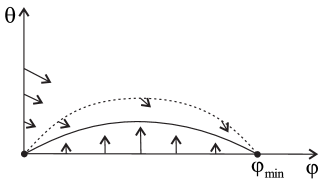
Figure 3. Boundary dynamics between a maximum of $S$ (at $\varphi=0$) and a minimum in case $T=\infty$: The dotted line is the graph of the barrier function $f$, the solid line is the trajectory $\Gamma_{{\bf p}_{-}}$

Since $\dot{\varphi}=\theta>0$ in the first quadrant, $\varphi$ is strictly increasing on $(-\infty,T)$. Now there are two possibilities:

(31) either $$T<\infty,\text{ then $\varphi(T)=\varphi_{\text{min}}$ and $\theta(T)>0$}$$

or $$T=\infty,\text{ then $\varphi(t)<\varphi_{\text{min}}\ \forall t$ and $\varphi(t)\to\varphi_{\text{min}}$, $\theta(t)\to 0$ as $t\to\infty$}$$

(and hence $\Gamma_{{\bf p}_{-}}(t)\to{\overline{\bf p}}_{\text{min}}$), by Proposition 5.1 a) since there are no critical points with $\varphi\in(0,\varphi_{\text{min}})$.

We discuss the first case below in the proof of Theorem 1.5. In the second case in (31) the trajectory $\Gamma_{{\bf p}_{-}}$ is the graph of a smooth function $h:(0,\varphi_{\text{min}})\to(0,\infty)$. We now give a sufficient condition for this to occur. It is obtained by a simple barrier argument.

Lemma 5.3.

Suppose we are in the setup described above, starting from (29). Assume that there is a $C^{1}$ function $f:[0,\varphi_{\text{min}}]\to\mathbb{R}_{+}$ satisfying the conditions

(32) $$f(\varphi_{\text{min}})=0,\text{ and }f(\varphi)>0\text{ for }\varphi\in(0,\varphi_{\text{min}})$$

(33) $$f(0)>0,\text{ or }f(0)=0\text{ and }f^{\prime}(0)>\lambda_{2}({\bf p}_{-}).$$

(34) $$ff^{\prime}+3f+S_{\varphi}\geq 0\text{ on }(0,\varphi_{\text{min}})$$

Then:

1. The closure of the image of $\Gamma_{{\bf p}_{-}}$ is the graph of a $C^{1}$ function $h:[0,\varphi_{\text{min}}]\to\mathbb{R}_{+}$, and $h^{\prime}(0)=\lambda_{2}({\bf p}_{-})$.

2. If in addition $(ff^{\prime}+3f+S_{\varphi})^{\prime}<0$ at $\varphi_{\text{min}}$ then $\Gamma_{{\bf p}_{-}}$ approaches ${{\bf p}_{\text{min}}}$ tangent to the eigenvector $\nu_{2}({{\bf p}_{\text{min}}})$, that is, $h^{\prime}(\varphi_{\text{min}})=\lambda_{2}({{\bf p}_{\text{min}}})$.

Concerning the condition in b), observe that $f(\varphi_{\text{min}})=0$ implies differentiability of $ff^{\prime}$ there, with derivative $(f^{\prime}(\varphi_{\text{min}}))^{2}$. Also, the function $g=ff^{\prime}+3f+S_{\varphi}$ satisfies $g(\varphi_{\text{min}})=0$ and $g(\varphi)\geq 0$ for $\varphi<\varphi_{\text{min}}$, which implies that $g^{\prime}(\varphi_{\text{min}})\leq 0$. The given condition strengthens this to $g^{\prime}(\varphi_{\text{min}})<0$.

Proof.

Let

$$D(f)=\{(\varphi,\theta):0\leq\varphi\leq\varphi_{\text{min}},\ 0\leq\theta\leq f(\varphi)\}$$

We claim that the vector field ${\bf V}=\theta\partial_{\varphi}-(S_{\varphi}+3\theta)\partial_{\theta}$ points inside $D(f)$, or is tangential to the boundary, at each boundary point of $D(f)$: This was checked before the proposition for the parts of the boundary where $\theta=0$ or $\varphi=0$. The remaining part of the boundary is the graph of $f$, which is the zero set of $\tilde{f}(\varphi,\theta)=f(\varphi)-\theta$, with $\tilde{f}>0$ inside $D(f)$. Now ${\bf V}\tilde{f}=\theta f^{\prime}+S_{\varphi}+3\theta$, which at $\theta=f(\varphi)$ equals $ff^{\prime}+3f+S_{\varphi}$, so (34) gives ${\bf V}\tilde{f}\geq 0$ which was to be shown.

By (33) the trajectory $\Gamma_{{\bf p}_{-}}$ starts out into the interior of $D(f)$, and by what we just proved it can never leave it. Since $\dot{\varphi}=\theta$ is positive in the interior of $D(f)$, the trajectory traces out the graph of a smooth function $\varphi\mapsto h(\varphi)$ on $(0,\varphi_{\text{min}})$. $h$ extends to be smooth at $0$ by the unstable manifold theorem, and it is $C^{1}$ at $\varphi_{\text{min}}$ since the trajectory is tangent to an eigenspace at ${\overline{\bf p}}_{\text{min}}$. This proves a).

Finally, $(ff^{\prime}+3f+S_{\varphi})^{\prime}=(f^{\prime})^{2}+3f^{\prime}+S_{\varphi\varphi}$ at $\varphi_{\text{min}}$, and if this is negative then $f^{\prime}$ (everything evaluated at $\varphi_{\text{min}}$) must lie strictly between the zeroes $\lambda_{2}$ and $\lambda_{3}$ of the characteristic polynomial $\lambda^{2}+3\lambda+S_{\varphi\varphi}$ of the linear part of ${\bf V}$ at $\varphi_{\text{min}}$, so $h^{\prime}\geq f^{\prime}>\lambda_{3}$. Since $h^{\prime}$ must be either $\lambda_{2}$ or $\lambda_{3}$ by the local behavior of trajectories, it follows that $h^{\prime}=\lambda_{2}$ and hence b). ∎

Proposition 5.4.

Let $M$ be a cuspidal surface of order $2$ and assume $S$ is a Morse function on $\partial M$ satisfying the bound $S_{\varphi\varphi}<9/4$ everywhere, where $\varphi$ is an arc length parameter on $\partial M$. Let $\Gamma=\bigcup_{\bf p}\Gamma_{\bf p}$ where ${\bf p}$ ranges over the critical points of $S$ and $\Gamma_{\bf p}$ is the unstable manifold of the point ${\overline{\bf p}}$ for the vector field ${\bf V}$ on $T^{*}\partial M$. Then $\Gamma$ is the graph of a $C^{1}$ section of $T^{*}\partial M$. That is,

$$\Gamma=\{(\varphi,\theta):\,\varphi\in\partial M,\ \theta=h(\varphi)\},\quad h\in C^{1}(\partial M).$$

Furthermore, $h^{\prime}(\varphi)=\lambda_{2}({\bf p}(\varphi))$ at each critical point ${\bf p}={\bf p}(\varphi)$ of $S$.

In fact, the proof shows that $h$ is $C^{\infty}$ except at minima of $S$, and at the minima the regularity can, in general, be slightly improved, see the remark after Proposition 6.4.

Proof.

Since $S$ is a Morse function and $\dim\partial M=1$, its critical points are either maxima or minima, and these alternate along $\partial M$. We first consider an interval between a maximum ${\bf p}_{-}$ and the next minimum ${{\bf p}_{\text{min}}}$. We may assume that the maximum is at $\varphi=0$ and the minimum is at $\varphi_{\text{min}}>0$. Then we are in the situation of Lemma 5.3. As barrier function we take $f=-\tfrac{2}{3}S_{\varphi}$. This clearly satisfies condition (32). Also, condition (34) holds since

$$g:=ff^{\prime}+3f+S_{\varphi}=\tfrac{4}{9}S_{\varphi}S_{\varphi\varphi}-2S_{\varphi}+S_{\varphi}=S_{\varphi}(\tfrac{4}{9}S_{\varphi\varphi}-1)>0$$

on $(0,\varphi_{\text{min}})$, and $g^{\prime}(\varphi_{\text{min}})<0$ since $S_{\varphi}=0$, $\tfrac{4}{9}S_{\varphi\varphi}-1<0$, $S_{\varphi\varphi}>0$ at $\varphi_{\text{min}}$. Finally, since $f(0)=0$ condition (33) is equivalent to $-\tfrac{2}{3}a>\tfrac{-3+\sqrt{9-4a}}{2}$ where $a=S_{\varphi\varphi}(0)$, which is easily checked to be true for any $a<0$. So Lemma 5.3 a) and b) are applicable and yield a function $h_{{\bf p}_{-}{{\bf p}_{\text{min}}}}$ on the interval $[0,\varphi_{\text{min}}]$ satisfying the claim of the Proposition there. We construct corresponding functions for each pair $({\bf p}_{-},{{\bf p}_{\text{min}}})$ of consecutive maxima and minima of $S$, and by changing the signs also for pairs $({{\bf p}_{\text{min}}},{\bf p}_{+})$ of consecutive minima and maxima; here $h_{{{\bf p}_{\text{min}}}{\bf p}_{+}}$ is negative in the interior of this interval. All these functions fit together to form a continuous function $h$ on all of $\partial M$ since they vanish at the endpoints of these intervals. $h$ is smooth at maxima ${\bf p}$ of $S$ since its graph is the unstable manifold of ${\overline{\bf p}}$ near ${\overline{\bf p}}$, which is smooth. $h$ is $C^{1}$ at minima ${{\bf p}_{\text{min}}}$ of $S$ since its derivatives from both sides agree, by Lemma 5.3b). ∎

The value $\tfrac{9}{4}$ is optimal for this type of barrier function $f$. Note that the condition $0<S_{\varphi\varphi}<\frac{9}{4}$ at a minimum ${{\bf p}_{\text{min}}}$ is equivalent to the linear part of ${\bf V}$ at ${{\bf p}_{\text{min}}}$ having two distinct negative real eigenvalues.

See Section 7 for a sufficient condition when the condition of Proposition 5.4 is satisfied in the case of cuspidal singularities.

Adjustments for general order $k$

The discussion generalizes to general $k$ by replacing $S$ with $\frac{1}{2}k(k-1)S$ and $3$ by $2k-1$, starting in (25), (26). Compare (21). Proposition 5.1 generalizes literally (with obvious adjustments in the proof). In the statement of Lemma 5.3 replace $S$ and $3$ as described.

In Proposition 5.4 the bound $S_{\varphi\varphi}<9/4$ is replaced by $S_{\varphi\varphi}<a_{k}$, with $a_{k}$ defined in (4). This results from replacing the barrier function $f=-\frac{2}{3}S_{\varphi}$ by $f=-\frac{k(k-1)}{2k-1}S_{\varphi}$.

6. The exponential map in the case of a Morse function $S$

In this section we prove Theorem 1.1 for cuspidal manifolds of arbitrary dimension with $S$ a constant or a Morse function. Then we consider the case of a cuspidal surface, with $S$ a Morse function. We define the exponential map and prove Theorems 1.3, 1.4 and 1.5.

Proof of Theorem 1.1

Assume $k=2$ first. The geodesics are, up to reparametrization, the projections to $M$ of the integral curves of the vector field ${\bf V}$ on the energy hypersurface $\{E=\tfrac{1}{2}\}\subset{}^{\text{3}}T^{*}M$. Thus, let $\gamma:(T_{-}^{\prime},T_{+}^{\prime})\to{}^{\text{3}}T^{*}M$ be a maximal integral curve of ${\bf V}$, and assume that $\gamma_{|(T_{-}^{\prime},T^{\prime})}$ is contained in $\{r<r_{0}\}$ for some $T^{\prime}\in(T_{-}^{\prime},T_{+}^{\prime})$. The number $r_{0}$ will be chosen sufficiently small below. Then necessarily $T_{-}^{\prime}=-\infty$ since ${\bf V}$ is tangent to the boundary. We will show that $\lim_{t\to-\infty}\gamma(t)$ exists and is a singular point of ${\bf V}$.

Write $\gamma(t)=(r(t),\varphi(t),\xi(t),\theta(t))$. Here we have chosen a trivialization of $M$ near the boundary, which allows us to identify ${}^{\text{3}}T^{*}M$ with $T^{*}[0,r_{0})\times T^{*}\partial M$ there, and then $(r,\xi)$ denotes a point in the first factor and $(\varphi,\theta)$ a point in the second factor. The proof falls into two parts: First, we use the $\dot{r}$ and $\dot{\xi}$ equations in (18) to show that $\xi(t)$ must be close to one on $(-\infty,T^{\prime})$, hence $r(t)$ exponentially decreasing as $t$ decreases, and that $\theta(t)$ is bounded. Then the decay of $r$ together with the boundedness of $\theta$ shows that the $\dot{\varphi}$, $\dot{\theta}$ dynamics is close to the boundary dynamics, which allows us to use Proposition 5.1b).

By (18) there is $K>0$ such that $\dot{\xi}\geq 2(1-\xi^{2})-Kr$ on the energy hypersurface.

Claim 1: $\xi>\frac{1}{2}$ for $t<T^{\prime}$.

Proof.

For $r_{0}$ sufficiently small we have $\dot{\xi}>1$ for $|\xi|\leq\frac{1}{2}$, so if $\xi(t_{0})\leq\frac{1}{2}$ for some $t_{0}<T^{\prime}$ then $\xi(t)<-\frac{1}{2}$ for all $t<t_{0}-1$, and then $\dot{r}=\xi r+O(r^{3})$ implies that $r$ leaves the interval $[0,r_{0}]$ as $t\to-\infty$, if $r_{0}$ is chosen sufficiently small (depending on the constant in $O(r^{3})$). This would contradict the assumption that $r(t)<r_{0}$ for all $t<T^{\prime}$. ∎

Claim 2: $\xi^{2}>1-Kr$ for $t<T^{\prime}$.

Proof.

Let $f(r,\xi)=\xi^{2}+Kr$. The part of $\gamma_{|(-\infty,T^{\prime})}$ where $f>1$ is forward invariant under the flow of ${\bf V}$, since at any point with $f(r,\xi)=1$, we have $2(1-\xi^{2})-Kr=Kr$ and therefore ${\bf V}f=2\xi\dot{\xi}+K\dot{r}\geq 2\xi(2(1-\xi^{2})-Kr)+K(r\xi+O(r^{3}))=3\xi Kr+O(r^{3})>0$, by Claim 1, for $r_{0}$ sufficiently small. Hence if $f\leq 1$ at some point $\gamma(t_{0})$ then this remains true for all $t\leq t_{0}$. Now $f(r,\xi)\leq 1$ implies $2(1-\xi^{2})-Kr\geq 1-\xi^{2}>0$, so we would get $\dot{\xi}>1-\xi^{2}>0$ for all $t\leq t_{0}$. Then $\xi$ would be monotone increasing in $t\leq t_{0}$, so $\lim_{t\to-\infty}\xi(t)$ would exist and lie in $[\frac{1}{2},1)$. However, this is impossible since it would imply $\xi(t_{0})-\xi(-\infty)>\int_{-\infty}^{t_{0}}(1-\xi(t)^{2})dt=\infty$ and hence unboundedness of $\xi$. ∎

Now we conclude from (17) and Claim 2 that $r\theta^{2}$ is bounded (everything for $t<T^{\prime}$). Using this in the $\dot{\xi}$ equation in (18) we see that in fact $\dot{\xi}\geq 2(1-\xi^{2})-Kr^{2}$, and then essentially the same argument as in Claim 2 shows that we even have $\xi^{2}>1-Kr^{2}$. This in turn, again in conjunction with (17), shows that $\theta$ is bounded. From Claim 1 and $\dot{r}=r\xi+O(r^{3})$ we obtain $r(t)\leq Ke^{-|t|/3}$. Also, (17) implies that $|\xi(t)-1|\leq K^{\prime}e^{-2|t|/3}$. Therefore Remark 5.2, applied to the $\dot{\varphi}$ and $\dot{\theta}$ equations in (18), implies that $\gamma(t)$ approaches a singular point of ${\bf V}$ as $t\to-\infty$. This proves parts (a) and (b) of Theorem 1.1.

The claim that each singular point ${\overline{\bf p}}$ of ${\bf V}$ is the starting point of a trajectory of ${\bf V}$ follows from the invariant manifold theorem and Lemma 4.1 since the unstable tangent space at ${\overline{\bf p}}$ contains the eigenvector for the eigenvalue $\lambda=1$, which points inside $M$.

Finally, returning to the unrescaled geodesic vector field we have $r^{\prime}=\xi+O(r^{2})$ along a geodesic, and since $\xi$ is near one this implies that the geodesic reaches $r=0$ in finite backward time, so $T_{-}$ is finite. Also, it implies that there is $\tau_{0}>0$ only depending on $r_{0}$ so that $r(t)<r_{0}$ for $t-T_{-}\leq\tau_{0}$, and this proves part (c).

This completes the proof of Theorem 1.1 in the case $k=2$. For general $k$ the proof is analogous, using ($\ref{eqn: energy shell}_{k}$), ($\ref{eq: diffeq E1 leading terms}_{k}$) instead of (17), (18).

Definition of the exponential map

We now define the exponential map in the case where $M$ is a cuspidal surface (of any order $k\geq 2$) with connected boundary ${\partial M}$ and $S$ is a Morse function on ${\partial M}$. For this we need to parametrize appropriately the family of geodesics starting at the points of ${\partial M}$. Recall that geodesics start at the critical points of the function $S$, and are projections of integral curves of the rescaled geodesic vector field ${\bf V}$ on the energy level $\{E=\frac{1}{2}\}\subset{}^{\text{3}}T^{*}M$ (resp. ${}^{(2k-1)}T^{*}M$).

The boundary ${\partial M}$ is diffeomorphic to a circle. Fixing an orientation of ${\partial M}$, we label the critical points of $S$ in cyclic order ${\bf p}_{1},{\bf p}_{1}^{\prime},{\bf p}_{2},{\bf p}_{2}^{\prime},\dots,{\bf p}_{l},{\bf p}_{l}^{\prime}$, where $l\in\mathbb{N}$ and where $S$ has maxima at the ${\bf p}_{i}$ and minima at the ${\bf p}_{i}^{\prime}$.

Recall the considerations in the proof of Proposition 4.2, in the case of surfaces: Each critical point ${\bf p}$ of $S$ is the projection of a hyperbolic singular point ${\overline{\bf p}}$ of ${\bf V}$. The geodesics hitting the boundary ${\partial M}$ in ${\bf p}$ are, as sets, the projections of the integral curves of ${\bf V}$ whose union form the interior of the unstable manifold $M^{u}_{\bf p}$ of ${\bf V}$ at ${\overline{\bf p}}$. This unstable manifold is two dimensional for each maximum ${\bf p}={\bf p}_{i}$ and projects diffeomorphically to $M$ in a neighborhood of ${\overline{\bf p}}_{i}$. It is one-dimensional for each minimum ${\bf p}={\bf p}_{i}^{\prime}$.

Recall from Theorem 1.1 that there is $\tau_{0}>0$ so that all geodesics starting at $\partial M$ exist at least for time $\tau_{0}$. In the following definition we consider the circle ${\bf S}^{1}$ as the interval $[0,2\pi]$ with the endpoints identified.

Definition 6.1.

Under the assumptions and with the notation introduced above we define the exponential map as follows:

1. For each maximum ${\bf p}_{i}$ of $S$ we parametrize the set of geodesics starting at ${\bf p}_{i}$ by the interval $I_{i}=\left(\frac{2(i-1)\pi}{l},\frac{2i\pi}{l}\right)\subset{\bf S}^{1}$, preserving orientation.

2. We let the unique geodesic starting at the minimum ${\bf p}_{i}^{\prime}$ of $S$ correspond to the point $\frac{2i\pi}{l}\in S^{1}$.

3. This defines a parametrization $q\mapsto\gamma_{q}$, $q\in{\bf S}^{1}$, of the geodesics starting at ${\partial M}$. Then we define

   $$\exp_{{\partial M}}:{\bf S}^{1}\times(0,\tau_{0})\to U\setminus{\partial M},\quad(q,t)\mapsto\gamma_{q}(\tau)$$

   where $\gamma_{q}$ is parametrized by arclength, starting at ${\partial M}$ at time $\tau=0$.

Note that we did not specify the precise parametrization in (1). The reason for this is that there is no natural parametrization. In fact, even the choice of intervals $I_{i}$ is arbitrary (apart from their ordering on the circle). More precisely, if $\kappa:{\bf S}^{1}\to{\bf S}^{1}$ is any orientation preserving homeomorphism, then $\exp^{\prime}_{\partial M}(q,\tau)=\exp_{\partial M}(\kappa(q),\tau)$ will serve just as well as exponential map. The set of exponential maps $\exp_{\partial M}(q,\tau)=\gamma_{q}(\tau)$ obtained in this way are characterized by the

Local order preserving property: If $a,b,c\in{\bf S}^{1}$ are pairwise different and lie in this order on ${\bf S}^{1}$ then there is $\tau_{1}>0$ so that the geodesics $\gamma_{a},\gamma_{b},\gamma_{c}$ do not intersect and lie in this order for times in $(0,\tau_{1})$.

Here, $\tau_{1}$ may depend on $a,b,c$, and for certain cuspidal metrics cannot be chosen uniformly for all $a,b,c$. This leads to discontinuity of the exponential map, see Remark 6.5.

In Remark 6.2 we sketch a more intrinsic definition of the exponential map, which makes use of a generalized notion of inhomogeneous blow-up.

To clarify part (1) of the definition, we now give an explicit parametrization using linearizations.

Let ${\bf p}={\bf p}_{i}$ be a maximum of $S$, and let $\tilde{U}\subset M_{\bf p}^{u}$ be a neighborhood of ${\overline{\bf p}}$ so that the projection $\pi:\tilde{U}\to M$ is a diffeomorphism to its image. The rescaled geodesic vector field ${\bf V}$ is tangent to $\tilde{U}$. Let ${\bf V}_{|\tilde{U}}$ be its restriction to $\tilde{U}$ and ${\bf V}^{\prime}=\pi_{*}({\bf V}_{|\tilde{U}})$ its projection to $\pi(\tilde{U})\subset M$. Since the linearization of ${\bf V}$ at ${\overline{\bf p}}$ has eigenvalues $1$ and $\lambda_{2}({\bf p})>0>\lambda_{3}({\bf p})$, the linearization of ${\bf V}_{|\tilde{U}}$ at ${\overline{\bf p}}$ has eigenvalues $1$ and $\lambda_{2}:=\lambda_{2}({\bf p})$. Then the same is true for the linearization of ${\bf V}^{\prime}$ at ${\bf p}$. Since both eigenvalus are positive, ${\bf V}^{\prime}$ is $C^{1}$-linearizable near ${\bf p}$ by Hartman’s Theorem [Har] (see also [Per, p 127]).

Therefore, we may choose $C^{1}$ coordinates $\rho\geq 0,\psi$ near ${\bf p}$, where $\rho=0$ on $\partial M$, so that in these coordinates ${\bf p}=(0,0)$ and ${\bf V}^{\prime}=\rho\partial_{\rho}+\lambda_{2}\psi\partial_{\psi}$. We may also assume that the coordinates are chosen so that the orientation of ${\partial M}$ corresponds to the positive $\psi$-direction. The integral curves (as sets) of ${\bf V}^{\prime}$ not contained in the boundary $\rho=0$ are of the form $\{\psi=K\rho^{\lambda_{2}},\rho>0\}$ with $K\in\mathbb{R}$. Therefore, $K$ parametrizes the family of integral curves of ${\bf V}^{\prime}$, hence of geodesic leaving ${\bf p}$, and does so in an order preserving way. Now choosing a diffeomorphism $\mathbb{R}\to I_{i}$, for example $K\mapsto\frac{\pi}{l}\left(\frac{K}{1+K^{2}}+2i-1\right)$, we get a parametrization as required in (1) of Definition 6.1.

Remark 6.2.

The domain of the parametrization $q\mapsto\gamma_{q}$ may be described somewhat more naturally with the help of the following construction: For a vector field ${\bf V}$ on a smooth manifold $\Sigma$ with an unstable critical point ${\bf p}$ there is a natural notion of blow-up of ${\bf p}$ in $\Sigma$ with respect to ${\bf V}$. This is a smooth manifold with boundary, denoted $[\Sigma,{\bf p}]_{\bf V}$, together with a blow-down map $\beta_{\bf p}:[\Sigma,{\bf p}]_{\bf V}\to\Sigma$. The boundary (front face) parametrizes the integral curves of ${\bf V}$ starting at ${\bf p}$. It is diffeomorphic to a sphere and may be thought of as small sphere around ${\bf p}$ transversal to ${\bf V}$. The map $\beta_{\bf p}$ may not be smooth, but ${\bf V}$ lifts to a smooth vector field on $[\Sigma,{\bf p}]_{\bf V}$, given by $s\partial_{s}$ near the boundary for a suitable boundary defining function $s$. The construction generalizes to the case where $\Sigma$ is a manifold with boundary, ${\bf p}\in\partial\Sigma$, and ${\bf V}$ is tangent to $\partial\Sigma$, and then yields a manifold with corners. See [HMV, Section 2] for details.

We apply this to the surface $M^{u}_{{\bf p}_{i}}$ for each $i$ and obtain $[M^{u}_{{\bf p}_{i}},{\overline{\bf p}}_{i}]_{\bf V}$. The front face $F_{i}:=\beta_{\bf p}^{-1}({\overline{\bf p}}_{i})$ of the blow-up is diffeomorphic to a closed interval, and is oriented by the orientation of ${\partial M}$. We now glue the right endpoint of each $F_{i-1}$ to the left endpoint of $F_{i}$ (with $F_{0}=F_{l}$) and obtain a manifold $F$ homeomorphic to ${\bf S}^{1}$ which is the natural domain of parametrization of geodesics leaving ${\partial M}$. Then the exponential map is defined on $F\times(0,\tau_{0})$.

The exponential map in the sense of Definition 6.1 is obtained by parametrizing the interior of $F_{i}$ by the interval $I_{i}$ for each $i$.

Proof of Theorem 1.3

We constructed the exponential map above. We need to show that it is surjective. For this we prove that the union of the unstable manifolds $M^{u}_{\bf p}$ over all critical points projects onto a neighborhood of $\partial M$ under the canonical projection $\pi:{}^{\text{3}}T^{*}M\to M$ (resp. $\pi:{}^{(2k-1)}T^{*}M\to M$ for general $k$).

First, observe that each unstable manifold $M_{\bf p}^{u}$ intersects the boundary $\{r=0\}$ transversally near ${\overline{\bf p}}$ since this is true for the linear part of ${\bf V}$, and since both $M_{\bf p}^{u}$ and $\{r=0\}$ are invariant under the flow, the intersection is transversal everywhere. The intersection $M_{\bf p}^{u}\cap\{r=0\}$ is the unstable manifold $\Gamma^{u}_{\bf p}$ of ${\overline{\bf p}}$ of ${\bf V}$ restricted to the boundary.

The projections of the unstable manifolds $M^{u}_{{\bf p}_{i}^{\prime}}$ are (closures of) single geodesics starting at ${\bf p}_{i}^{\prime}$, which divide a neighborhood of ${\partial M}$ into connected components $U_{i}$, each containing one maximum ${\bf p}_{i}$. It suffices to show that $\pi(M^{u}_{{\bf p}_{i}})$ contains $U_{i}$ for each $i$.

For this, first consider the intersections with the boundary. Fix $i$ and write ${\bf p}_{-}={\bf p}_{i}$ and ${{\bf p}_{\text{min}}}={\bf p}_{i}^{\prime}$. By the discussion before Lemma 5.3, the part $\Gamma_{{\bf p}_{-}}$ of $\Gamma^{u}_{{\bf p}_{-}}$ leaving ${\bf p}_{-}$ in the positive $\varphi$ direction projects onto the (open) interval from ${\bf p}_{-}$ to ${{\bf p}_{\text{min}}}$. A similar statement holds for the interval from ${\bf p}_{i-1}^{\prime}$ to ${\bf p}_{-}$. Therefore, $M^{u}_{{\bf p}_{i}}\cap\{r=0\}$ projects onto $U_{i}\cap\{r=0\}$. Since $M^{u}_{{\bf p}_{i}}$ intersects the boundary transversally, it projects onto some neighborhood of the open interval from ${\bf p}_{i-1}^{\prime}$ to ${\bf p}_{i}^{\prime}$. We need to show that this neighborhood cannot shrink to zero width when one approaches ${\bf p}_{i-1}^{\prime}$ or ${\bf p}_{i}^{\prime}$. We will prove that $U_{i}$ intersected with a neighborhood of ${\bf p}_{i}^{\prime}$ is contained in $\pi(M^{u}_{{\bf p}_{i}})$; the argument at ${\bf p}_{i-1}^{\prime}$ is then analogous.

Recall the dichotomy (31). If $T<\infty$ here then $\pi(\Gamma_{{\bf p}_{-}})$ contains ${\bf p}_{i}^{\prime}$, so we are done. On the other hand, if $T=\infty$ then $\Gamma_{{\bf p}_{-}}(t)\to{\overline{\bf p}}_{\text{min}}$ as $t\to\infty$, and the eigenvalues $\lambda_{2}({{\bf p}_{\text{min}}})$, $\lambda_{3}({{\bf p}_{\text{min}}})$ are real. In this case, the behavior of $M^{u}_{{\bf p}_{-}}$ near ${\overline{\bf p}}_{\text{min}}$ may be understood by linearizing ${\bf V}$ near ${\overline{\bf p}}_{\text{min}}$. We use Lemma 6.3 below, applied as explained after its statement. For later purposes the lemma is stated more strongly than needed here. Here we only need the consequence that, in a neighborhood of ${\overline{\bf p}}_{\text{min}}$, the curve $M^{u}_{{\bf p}_{\text{min}}}$ is contained in the closure of $M^{u}_{{\bf p}_{-}}$, so the projection of $M^{u}_{{\bf p}_{\text{min}}}$ is contained in the closure of $U_{i}$. This completes the proof of Theorem 1.3.

Lemma 6.3.

Let $\lambda,\mu<0$ and let $V$ be the linear vector field $x_{1}\partial_{x_{1}}+\lambda x_{2}\partial_{x_{2}}+\mu x_{3}\partial_{x_{3}}$ on $\mathbb{R}^{3}$. Let $m\geq 1$. Let $\Sigma$ be an invariant $C^{m}$ surface with boundary $\Gamma=\Sigma\cap\{x_{1}=0\}$, and assume this intersection is transversal and $\Gamma$ is a single trajectory of $V$. Denote by $X_{1}$ the non-negative $x_{1}$-axis.

Then a neighborhood $\Sigma^{\prime}$ of zero in $\Sigma\cup X_{1}$ is a surface with corner. More precisely, let $\tau=-\frac{1}{\lambda}$ and $\rho=\frac{\mu}{\lambda}$, so $\tau,\rho>0$. Assume $\Gamma\subset\{x_{2}>0\}$. Then $\Sigma^{\prime}$ is a graph

(35) $$\begin{gathered}\Sigma^{\prime}=\{(x_{1},x_{2},x_{3}):\ x_{3}=A(x_{1}x_{2}^{\tau})x_{2}^{\rho},\ (x_{1},x_{2})\in U^{\prime}\}\end{gathered}$$

where $A$ is a $C^{m}$ function on $[0,\varepsilon)$ for some $\varepsilon>0$, and $U^{\prime}$ is a neighborhood of the origin in the quarter plane $\mathbb{R}_{+}\times\mathbb{R}_{+}$.

The lemma is applied as follows, in the context of the discussion before Lemma 5.3: Let ${{\bf p}_{\text{min}}}$ be a minimum of $S$, and suppose the second alternative in (31) holds. Then $\Gamma_{{\bf p}_{-}}(t)$ approaches ${\overline{\bf p}}_{\text{min}}$ as $t\to\infty$. By Proposition 4.4 we may linearize ${\bf V}$ near ${\overline{\bf p}}_{\text{min}}$ by a $C^{m}$-diffeomorphism where $m\in\{1,2\}$. Thus, we introduce local coordinates $x_{1},x_{2},x_{3}$ so that ${\overline{\bf p}}_{\text{min}}$ is the origin and ${\bf V}$ is given by $x_{1}\partial_{x_{1}}+\lambda x_{2}\partial_{x_{2}}+\mu x_{3}\partial_{x_{3}}$ on a neighborhood $U$ where $\{\lambda,\mu\}=\{\lambda_{2}({{\bf p}_{\text{min}}}),\lambda_{3}({{\bf p}_{\text{min}}})\}$ and the boundary is given by $\{x_{1}=0\}$. We take $\Gamma=\Gamma_{{\bf p}_{-}}$ and $\Sigma=M^{u}_{{\bf p}_{-}}$. Clearly $M^{u}_{{{\bf p}_{\text{min}}}}=X_{1}$. Since $\Gamma$ is a trajectory of ${\bf V}$ approaching the origin, it must have a tangent vector there, and we may assume that the coordinates are chosen so that this vector is $\partial_{x_{2}}$. Then $\Gamma\subset\{x_{2}>0\}$ near the origin, so the assumptions of the lemma are satisfied.

Proof of Lemma 6.3.

Choose a point $p$ of $\Gamma$. Since the intersection of $\Sigma$ with $\{x_{1}=0\}$ is transversal we may choose a $C^{m}$-curve $\omega(s)=(s,\omega_{2}(s),\omega_{3}(s))$, $s\in I=[0,\varepsilon)$ contained in $\Sigma$, with $\omega(0)=p$, so $\omega_{2}(0)>0$. Also, since $x_{1}x_{2}^{\tau}$ is constant along any integral curve of ${\bf V}$, only trajectories passing through this curve will contribute to $\Sigma^{\prime}$ if this is chosen sufficiently small.

For $s\in I$ let $\mathbb{R}_{+}\to\mathbb{R}^{3}$, $t\mapsto\Gamma_{s}(t)$ be the forward integral curve of ${\bf V}$ starting at $\omega(s)$, so $\Gamma_{s}(0)=\omega(s)$ and $\Gamma_{0}=\Gamma$, up to time shift.

For each $s$, the quantities $x_{1}x_{2}^{\tau}$ and $x_{3}x_{2}^{-\rho}$ are constant along $\Gamma_{s}$, that is, for points $(x_{1},x_{2},x_{3})$ in the image of $\Gamma_{s}$. Evaluating at $t=0$ shows that, along $\Gamma_{s}$,

(36) $$x_{1}x_{2}^{\tau}=s\omega_{2}(s)^{\tau},\quad x_{3}x_{2}^{-\rho}=\omega_{3}(s)\omega_{2}(s)^{-\rho}.$$

Now $\omega_{2}(0)>0$, hence the equation $\sigma=s\omega_{2}(s)^{\tau}$ can be solved $C^{m}$-smoothly for $s=s(\sigma)$, for $\sigma$ in a half neighborhood $J$ of zero, and the function $A:J\to\mathbb{R}$, $\sigma\mapsto\omega_{3}(s(\sigma))\omega_{2}(s(\sigma))^{-\rho}$ is $C^{m}$. Then we have along $\Gamma_{s}$, with this $\sigma$,

$$x_{3}=A(\sigma)x_{2}^{\rho}=A(x_{1}x_{2}^{\tau})x_{2}^{\rho}.$$

The claim follows. ∎

Proof of Theorem 1.4

Assume $k=2$ first. The heart of the proof is that the various unstable manifolds fit together nicely. So we first prove the following proposition.

Proposition 6.4.

Assume the setting and the conditions of Theorem 1.4. Let $M^{u}$ be the union of the unstable manifolds $M_{\bf p}^{u}$, where ${\bf p}$ ranges over the critical points of $S$. Then $M^{u}$ is a $C^{1}$ manifold, and there is $r_{0}>0$ so that the intersection of $M^{u}$ with $\{r<r_{0}\}$ projects diffeomorphically to $M\cap\{r<r_{0}\}$ under the projection $\pi:{}^{\text{3}}T^{*}M\to M$.

See Figure 4.

The proof actually gives more regularity than $C^{1}$: The manifold $M^{u}$ is $C^{\infty}$ except at points on the curves $M_{\bf p}^{u}$ where ${\bf p}$ is a minimum of $S$, and here the regularity is $C^{\alpha({\bf p})}$ where

(37) $$\alpha({\bf p})=\begin{cases}1&\text{ if }\lambda_{2}\in\mathbb{Q}\\ \min\{2,\frac{\lambda_{3}}{\lambda_{2}}\}&\text{ if }\lambda_{2}\in\mathbb{R}\setminus\mathbb{Q}\end{cases}$$

with $\lambda_{2}=\lambda_{2}({\bf p})$, $\lambda_{3}=\lambda_{3}({\bf p})$.

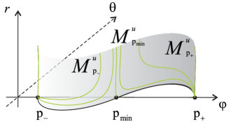
Figure 4. The dynamics near the boundary.

Proof of Proposition 6.4.

The main task is to prove that the different $M_{\bf p}^{u}$ fit together to form a $C^{1}$ manifold, the projection statement will then be seen to be an easy consequence.

Since integral curves do not intersect, the manifolds $M_{\bf p}^{u}$ do not intersect for different ${\bf p}$. Since $M^{u}$ is invariant under the flow, it is enough to prove the regularity near $r=0$.

First consider the boundaries $\Gamma_{\bf p}^{u}=\partial M_{\bf p}^{u}=M_{\bf p}^{u}\cap\{r=0\}$ and their union $\Gamma^{u}=\bigcup_{\bf p}\Gamma_{\bf p}^{u}$. These are the unstable manifolds of ${\bf V}$ restricted to the boundary $T^{*}\partial M$. By assumption $S_{\varphi\varphi}<\frac{9}{4}$ everywhere, so we may apply Proposition 5.4 and conclude that $\Gamma$ is the graph of a $C^{1}$ function $\Gamma=\{(\varphi,h(\varphi)):\,\varphi\in\partial M\}$. Thus, both the regularity and the projection statement of Proposition 6.4 are true for the boundary of $M^{u}$.

We now prove that $M^{u}$ is a $C^{1}$ manifold in a neighborhood of $r=0$, with boundary $\Gamma^{u}$. Since $M_{\bf p}^{u}$ is a smooth surface for each maximum ${\bf p}$ of $S$, we only need to prove the regularity in a small neighborhood $U$ of ${\overline{\bf p}}_{\text{min}}$ where ${{\bf p}_{\text{min}}}$ is a minimum of $S$. Thus, let ${{\bf p}_{\text{min}}}$ be a minimum of $S$ and let ${\bf p}_{-}$, ${\bf p}_{+}$ be the maxima of $S$ closest to ${{\bf p}_{\text{min}}}$, so that the corresponding parameter values satisfy $\varphi_{-}<\varphi_{\text{min}}<\varphi_{+}$. Then the set $M^{u}\cap U$ is the union of $M_{{\bf p}_{-}}^{u}\cap U$, $M_{{{\bf p}_{\text{min}}}}^{u}\cap U$ and $M_{{\bf p}_{+}}^{u}\cap U$. We now apply Lemma 6.3 as explained after its statement, first to $\Sigma_{-}=M_{{\bf p}_{-}}^{u}\cap U$ and then to $\Sigma_{+}=M_{{\bf p}_{+}}^{u}\cap U$. By the last statement of Proposition 5.4, $\Gamma_{{\bf p}_{\pm}}$ have tangents $\pm\nu_{2}({{\bf p}_{\text{min}}})$ at ${\overline{\bf p}}_{\text{min}}$, so we take $\lambda=\lambda_{2}({{\bf p}_{\text{min}}})$, $\mu=\lambda_{3}({{\bf p}_{\text{min}}})$ in Lemma 6.3, and this implies $\rho>1$ there. The lemma shows that $\Sigma_{\pm}$ are graphs as in (35), with possibly different functions $A_{\pm}$.

The more precise regularity statement (37) follows from the regularity in Lemma 6.3 together with the regularity of the linearization, Proposition 4.4.

Finally we prove that $M^{u}$ projects diffeomorphically to $M$ near $r=0$. For any boundary point ${\overline{\bf q}}\in\Gamma^{u}={\partial M}^{u}$, the tangent space $T_{\overline{\bf q}}M^{u}$ is transversal to $\{r=0\}$, since this is already true for each $M_{\bf p}^{u}$ separately. In addition, $T_{\overline{\bf q}}M^{u}\supset T_{\overline{\bf q}}\Gamma^{u}$, so $T_{\overline{\bf q}}M^{u}\cap T_{\overline{\bf q}}\{r=0\}$ contains a vector with nonzero $\partial_{\varphi}$-component. These two facts combine to show that, for each ${\overline{\bf q}}\in{\partial M}^{u}$, the tangent space $T_{\overline{\bf q}}M^{u}$ projects isomorphically to $T_{\bf q}M$ under $d\pi$, where $\pi:{}^{\text{3}}T^{*}M\to M$ is the projection, and this implies the claim. ∎

We now prove Theorem 1.4. By Theorem 1.1 every geodesic starting at $\partial M$ must do so at a critical point ${\bf p}$ of $S$, so the corresponding integral curve of ${\bf V}$ starts at a singular point ${\overline{\bf p}}$ of ${\bf V}$. This integral curve is then contained in the unstable manifold $M_{\bf p}^{u}$ of ${\overline{\bf p}}$. Conversely, $M_{\bf p}^{u}\cap\{r>0\}$ is the union of such integral curves. Therefore, Proposition 6.4 implies that $\exp_{{\partial M}}$ is bijective.

It remains to prove the continuity of $\exp_{{\partial M}}$ and of its inverse. We continue to work on $M^{u}$. Some care needs to be taken since the vector field ${\bf W}$ blows up at the boundary. But the main point is that only its $\partial_{\varphi}$ component blows up, while its $\partial_{r}$ component is $\xi+O(r^{2})=1+O(r^{2})$. Recall that the domain of $\exp_{{\partial M}}$ is the set of $(q,\tau)$ where $\tau\in(0,\tau_{0})$ and $q$ is a point on a transversal $T_{i}$ near ${\overline{\bf p}}_{i}$ for some $i$, where the transversals are glued at their endpoints. The continuity of $\exp_{{\partial M}}$ at points $(q_{0},\tau)$ where $q_{0}$ is not a boundary point of a transversal $T_{i}$ is clear, so we assume that $q_{0}$ is a boundary point of $T_{i}$, say the ’right’ boundary point, which labels the geodesic starting at the next minimum ${\bf p}_{i}^{\prime}$. The idea is this: As sets, the geodesics $\gamma_{q}$, with $q$ in the interior of $T_{i}$ approaching $q_{0}$, converge to the union of the boundary trajectory $\Gamma_{{\bf p}_{i}}$ and of $M^{u}_{{\bf p}_{i}^{\prime}}$. Since $r^{\prime}=\frac{dr}{d\tau}$ is approximately one, the part of $\gamma_{q}$ near $\Gamma_{{\bf p}_{i}}$ is traversed in a very short time. Then the part near $M^{u}_{{\bf p}_{i}^{\prime}}$ must, including its time parametrization, be close to $\gamma_{q_{0}}$.

More precisely, fix $(q_{0},\tau)$ and a neighborhood $U$ of $\gamma_{q_{0}}(\tau)$. Denote by $r$, $r_{0}$ the $r$-components of integral curves $\gamma$, $\gamma_{q_{0}}$ of ${\bf W}$. Then there are $\delta>0$, a neighborhood $U^{\prime}$ of $M^{u}_{{\bf p}_{i}^{\prime}}$ and a neighborhood $V^{\prime}$ of $\tau$ so that for all $0<\tau_{1}<\tau$ and all integral curves $\gamma$ of ${\bf W}$ lying in $U^{\prime}$ for the time interval $(\tau_{1},\tau)$ and satisfying $|r(\tau_{1})-r_{0}(\tau_{1})|<\delta$ we have that $\gamma(\tau^{\prime})\in U$ for all $\tau^{\prime}\in V^{\prime}$. This is because $r^{\prime}=F(r,\varphi,\theta)$ where $F$ is $C^{1}$ and the values of $\varphi,\theta$ for $\gamma$ and $\gamma_{0}$ will be close together at all times in $(\tau_{1},\tau)$ if $U^{\prime}$ is chosen sufficiently small.

Next, for the $\delta>0$ and neighborhood $U^{\prime}$ of $M^{u}_{{\bf p}_{i}^{\prime}}$ obtained above there is a neighborhood $V$ of $q_{0}$ in $T_{i}$ so that for all $q\in V$ the curve $\gamma_{q}$ first runs inside $\{r<\delta/2\}$ and then inside $U^{\prime}$. Now $\frac{dr}{d\tau}=1+O(r^{2})$ implies that the travel time $\tau_{1}(q)$ for the first part is at most on the order of $\delta/2$. Then the $r$-components $r_{q}$ and $r_{0}$ of $\gamma_{q}$, $\gamma_{q_{0}}$ satisfy $|r_{q}(\tau_{1}(q))-r_{0}(\tau_{1}(q))|<\delta$, so the first part of the argument can be applied with $\gamma=\gamma_{q}$ and $\tau_{1}=\tau_{1}(q)$. Summarizing, given any neighborhood $U$ of $\gamma_{0}(\tau)$ we have found neighborhoods $V$ of $q_{0}$ and $V^{\prime}$ of $\tau$ so that $\gamma_{q}(\tau^{\prime})\in U$ for all $q\in V$, $\tau^{\prime}\in V^{\prime}$. This proves the continuity of $\exp_{{\partial M}}$, from the left with respect to $q$. Continuity from the right follows by the same argument applied to the left endpoint of $T_{i+1}$. The continuity of the inverse is proved in a similar way, but easier. For example, the second component, $\tau$, of $\exp_{{\partial M}}^{-1}$ is simply the distance to the boundary, and its continuity follows from the triangle inequality.

This concludes the proof of Theorem 1.4 in the case $k=2$. The argument for general $k$ is exactly the same, except that one replaces ${}^{\text{3}}T^{*}M$ by ${}^{(2k-1)}T^{*}M$, and in the proof of Proposition 6.4 one uses the condition $S_{\varphi\varphi}<a_{k}$ instead of $S_{\varphi\varphi}<9/4$ when referring to Proposition 5.4.

Remark 6.5.

The proof also shows why the exponential map may be discontinuous in general: Suppose $l\geq 2$ in Definition 6.1, i.e. the function $S$ has at least two maxima and at least two minima. Suppose $\Gamma_{{\bf p}_{1}}$ does not approach ${\bf p}_{1}^{\prime}$ but rather continues in the upper half plane $\theta>0$ and then approaches ${\bf p}_{2}^{\prime}$. Examples of functions $S$ yielding this boundary dynamics can easily be constructed. Let $q_{1},q_{2}$ be the labels of the geodesics leaving ${\bf p}_{1}^{\prime}$, ${\bf p}_{2}^{\prime}$, respectively. Then, for any fixed $\tau>0$, the point $\gamma_{q}(\tau)$ will approach $\gamma_{q_{2}}(\tau)$ rather than $\gamma_{q_{1}}(\tau)$ as $q\to q_{1}$ from the left, so $\exp_{{\partial M}}$ is discontinuous at $(q_{1},\tau)$ for any $\tau>0$. Also, it is easy to see that this discontinuity cannot be removed by a simple reordering (i.e. by a different gluing prescription), which in any case would be unnatural since it would break up the order preserving property of $\exp_{{\partial M}}$.

Proof of Theorem 1.5

Let ${{\bf p}_{\text{min}}}$ be a point where $S$ has a local minimum and where $S_{\varphi\varphi}>a_{k}$. Then the eigenvalues $\lambda_{2}({{\bf p}_{\text{min}}})$, $\lambda_{3}({{\bf p}_{\text{min}}})$ are non-real with real part $-\frac{2k-1}{2}$, so nearby trajectories of ${\bf V}$ on $T^{*}\partial M$ spiral towards ${\overline{\bf p}}_{\text{min}}$.

Consider the maxima ${\bf p}_{-}$, ${\bf p}_{+}$ of $S$ closest to ${{\bf p}_{\text{min}}}$, where $\varphi_{-}<\varphi_{\text{min}}<\varphi_{+}$ for the corresponding parameters. W.l.o.g. we may assume $S(\varphi_{-})\leq S(\varphi_{+})$. Then we are in the situation discussed before Lemma 5.3 (where we put $\varphi_{-}=0$ for simplicity), more precisely in the first case of (31). We claim that the trajectory $\Gamma_{{\bf p}_{-}}$ considered there approaches ${\overline{\bf p}}_{\text{min}}$ as $t\to\infty$. To show this, recall from the proof of Proposition 5.1 that the boundary energy function $\frac{1}{2}k(k-1)S(\varphi)+\theta^{2}/2$ and hence $S(\varphi)+\frac{1}{k(k-1)}\theta^{2}$ is strictly decreasing along $\Gamma_{{\bf p}_{-}}$. At $t=-\infty$ this function has the value $S(\varphi_{-})$, and on the line $\varphi=\varphi_{+}$ its values are at least $S(\varphi_{+})\geq S(\varphi_{-})$. Hence, $\Gamma_{{\bf p}_{-}}$ can not cross or approach this line, and neither the line $\varphi=\varphi_{-}$. So the only possible limit point of $\Gamma_{{\bf p}_{-}}$ for $t\to\infty$ is ${\overline{\bf p}}_{\text{min}}$, which was to be shown.

Now note that the spiraling of $\Gamma_{{\bf p}_{-}}$ around ${\overline{\bf p}}_{\text{min}}$ as $t\to\infty$ implies that the projection of $\Gamma_{{\bf p}_{-}}$ to the $\varphi$-axis oscillates around $\varphi_{\text{min}}$ infinitely often.

Now consider the unstable manifold $M_{{\bf p}_{-}}^{u}$. The image of $\Gamma_{{\bf p}_{-}}$ is an open subset of $\partial M_{{\bf p}_{-}}^{u}$. By continuity of ${\bf V}$, for any $T>0$ and $\varepsilon>0$ there are interior trajectories of ${\bf V}$ contained in $M_{{\bf p}_{-}}^{u}$ that follow the boundary trajectory $\Gamma_{{\bf p}_{-}}$ within an error of $\varepsilon$ on the time interval $[0,T]$. In particular, for any $\varepsilon>0$ there is a trajectory $\gamma$ starting at ${\overline{\bf p}}_{-}$ whose projection to $M$ intersects the projection of the trajectory $M^{u}_{{\bf p}_{\text{min}}}$ at a point with $r<\varepsilon$. This proves the theorem.

7. Application to cuspidal singularities

The main motivation for defining cuspidal metrics is that they arise from cuspidal singularities. The notion of cuspidal singularity itself does not involve a metric. In this section we give two definitions of cuspidal singularity, prove their equivalence and show that the restriction of a smooth ambient metric to a cuspidal singularity yields a cuspidal metric upon resolution of the singularity, so the main theorems are applicable in this setting. Also, we interpret the quantities $S$ and ${\bf g}_{\partial M}$ for cuspidal singularities and give a sufficient condition for the exponential map to be a homeomorphism.

7.1. Definition of cuspidal singularities

We now discuss the notion of cuspidal singularity for subsets $X$ of a smooth manifold $Z$. Since this is a local notion, one may always think of $Z=\mathbb{R}^{n}$; however, it is useful to have an invariant geometric understanding.

Recall that the tangent cone $C(X,p)$ of a subset $X\subset\mathbb{R}^{n}$ at $p\in X$ is the set of limits of secant half-lines through $p$ from points in $X$:

$C(X,p):=\{r\nu:\,r>0,\nu\in{\bf S}^{n-1},\exists(p_{j})_{j}\in X\setminus\{p\}:p_{j}\to p$ and $\lim_{j}\frac{p_{j}-p}{|p_{j}-p|}=\nu\}$.

It is well-known and easy to check that for subsets $X$ of a manifold $Z$ the tangent cone at $p\in X$ is invariantly defined as a subset $C(X,p)\subset T_{p}Z$.

Definition 7.1.

Let $k\geq 2$, $k\in\mathbb{N}$. Let $X$ be a subset of a manifold $Z$ and $p\in X$. We say that $X$ has a cuspidal singularity of order $k$ at $p$ if

1. the tangent cone $C(X,p)$ is a half-line and

2. there are coordinates $(x_{1},\dots,x_{n-1},z)$ on a neighborhood $U\subset Z$ of $p$ in which $p=0$ and $C(X,p)=\mathbb{R}_{>0}\partial_{z}$, so that $X\cap U$ is given locally as in (2), (2’).

Here $\partial_{z}=(0,\dots,0,1)$. If these conditions are satisfied then we say that the singularity of $X$ at $p$ can be resolved by a blow-up of order $k$. Note that condition (b) implies that $(X\cap U)\setminus\{p\}$ is a submanifold of $Z$. Below we need another characterization of cuspidal singularities in terms of a standard (or first order) blow-up followed by a blow-up of order $k-1$, which also has the virtue of leading to a manifestly invariant characterization. To formulate this we recall some basic terminology.

7.1.1. Review of blow-up

The (oriented, first order) blow-up of a manifold $Z$ in a point $q\in Z$ is a geometric, coordinate free counterpart to introducing polar coordinates around $q$. By definition it is a manifold with boundary, denoted $[Z,q]$, together with a smooth map $\beta_{q}:[Z,q]\to Z$ (the blow-down map) which maps the boundary $\partial[Z,q]$ to $q$ and is a diffeomorphism from $[Z,q]\setminus\partial[Z,q]$ to $Z\setminus\{q\}$, and which is, locally near $\partial[Z,q]$ resp. $q$, given by the following model: $Z=\mathbb{R}^{n}$, $q=0$, and then $[Z,q]=\mathbb{R}_{+}\times{\bf S}^{n-1}$ and $\beta_{q}(r,\omega)=r\omega.$ Thus $\partial[Z,q]=\{0\}\times{\bf S}^{n-1}$ in the model. See [Mel] or [Gri1] for a more in-depth discussion, in particular of the coordinate invariance of this notion and of its generalization to manifolds with corners. Of this we only need the case where $Z$ is itself a manifold with boundary and $q\in\partial Z$. Then $[Z,q]$ is a manifold with corners; the local model is $Z=\mathbb{R}^{n-1}\times\mathbb{R}_{+}$, $q=0$, $[Z,q]=\mathbb{R}_{+}\times{\bf S}^{n-1}_{+}$, where ${\bf S}^{n-1}_{+}={\bf S}^{n-1}\cap(\mathbb{R}^{n-1}\times\mathbb{R}_{+})$ is the upper half sphere and $\beta_{q}$ is as before. In this case, $\beta_{q}$ maps $\{0\}\times{\bf S}^{n-1}_{+}$ to $0$ and is a diffeomorphism between the complements of these sets. In either case $\beta_{q}^{-1}(q)$ is called the front face of the blow-up.

Starting from a coordinate system for $Z$ near $q$, projective coordinates are defined for $[Z,q]$ as follows. The coordinates for $Z$ identify a neighborhood of $q$ with $\mathbb{R}^{n}$, with $q=0$. Denote the coordinates by $(x,z)$ where $x=(x_{1},\dots,x_{n-1})$. Then the projective coordinates $(y,z)$, $y=(y_{1},\dots,y_{n-1})\in\mathbb{R}^{n-1}$, $z\in\mathbb{R}_{+}$ are defined to be the unique coordinates on the ’upper half’ $U=\{(r,\omega)\in\mathbb{R}_{+}\times{\bf S}^{n-1}:\,\omega_{n}>0\}$ of $[\mathbb{R}^{n},0]$ in terms of which the blow-down map is $\beta_{q}(y,z)=(zy,z)$. (So informally $y_{j}=\frac{x_{j}}{z}$ for $j=1,\dots,n-1$. The relation to the $r,\omega$-variables is $y_{i}=\frac{r}{\omega_{n}}\omega_{i}$, $z=r\omega_{n}$, but this is not needed.) There are also projective coordinate systems covering the remainder of $[\mathbb{R}^{n},0]$, but we do not need them here.

The blow-up to order $k$ can be given a similar invariant description, denoted $\beta_{q}:[Z,q]_{k}\to Z$, and (2) is the blow-down map in order $k$ projective coordinates.

If $X\subset Z$ then the strict transform of $X$ under the blow-up of $q$ is the closure of the pre-image of $X\setminus\{q\}$, so $\beta_{q}^{*}X:=\overline{\beta_{q}^{-1}(X\setminus\{q\})}$. A p-submanifold (p for ’product type’) of a manifold with boundary $Z$ is a submanifold $X\subset Z$ such that $\partial X\subset\partial Z$ and $X$ hits $\partial Z$ transversally. This extends to manifolds with corners $Z$; we only need the straightforward case where $X$ intersects the boundary only in the interior of a boundary hypersurface.

7.1.2. Alternative characterization of cuspidal singularities

Let $Z$ be a manifold and $X\subset Z$ a subset. We say that $X$ has a conical singularity at $q\in X$ if it is resolved by blowing up $q$. That is, there is an open neighborhood $U\subset Z$ of $q$ so that the strict transform of $X\cap U$ is a p-submanifold of $[U,q]$. If $Z$ is a manifold with boundary and $q\in\partial Z$ then we also require non-tangency of $X$ to $\partial Z$, that is, that the boundary of the strict transform of $X\cap U$ be contained in the interior of the front face of $[U,q]$.

Lemma 7.2.

Let $X$ be a subset of a manifold $Z$ and $p\in X$. Let $Z^{\prime}=[Z,p]$ be the blow-up of $Z$ in $p$ with blow-down map $\beta_{p}:Z^{\prime}\to Z$. Then $X$ has a cuspidal singularity of order $k$ at $p$ if and only if its strict transform $X^{\prime}=\beta_{p}^{*}(X)\subset Z^{\prime}$ intersects $\partial Z^{\prime}$ in a single point $q$ and

• if $k=2$: $Z^{\prime}$ has a conical singularity at $q$

• if $k>2$: $Z^{\prime}$ has a cuspidal singularity of order $k-1$ at $q$.

Thus, the singularity of $X$ can be resolved by first blowing up $p$ and then blowing up $q$ to order $k-1$. The resolution is defined as the strict transform

(38) $${\widetilde{X}}=(\beta_{p}\circ\beta_{q})^{*}X.$$

By iteration, this implies that an order $k$ blow-up can be replaced by a sequence of $k$ standard blow-ups. We will not use this consequence.

Proof.

Since this is a local statement we may assume $Z=\mathbb{R}^{n}$, $p=0$. Denote $X^{\prime}=\beta_{p}^{*}(X)\subset Z^{\prime}=[\mathbb{R}^{n},p]$. Points of the front face $\partial Z^{\prime}$ correspond to directions at $p$, so $C(X,p)=\{r\nu:\,\nu\in X^{\prime}\cap\partial Z^{\prime},\ r>0\}$. Therefore, condition (a) of Definition 7.1 is equivalent to $X^{\prime}$ intersecting $\partial Z^{\prime}$ in a single point $q$. Assuming this is satisfied we may choose coordinates $(x,z)$, $x=(x_{1},\dots,x_{n-1})$ on $\mathbb{R}^{n}$ so that $C(X,p)=\mathbb{R}_{>0}\partial_{z}$. In the corresponding projective coordinates $(y,z)$, for which $\beta_{p}(y,z)=(zy,z)$, this corresponds to $q=0$.

The coordinates $(y,z)$ on $Z^{\prime}$ define projective coordinates $(u,z)$ on $[Z^{\prime},q]_{k-1}$, for which the blow-down map $[Z^{\prime},q]\to Z^{\prime}$ is given by $\beta_{q}(u,z)=(z^{k-1}u,z)$, hence $\beta_{p}(\beta_{q}(u,z))=(z^{k}u,z)$. Let $\tilde{X}\subset[Z^{\prime},q]_{k-1}$ be the strict transform of $X^{\prime}$ under the order $k-1$ blow-up of the manifold with boundary $Z^{\prime}$ in $q$. The coordinates $(u,z)$ are defined in a neighborhood of the interior of the front face of $[Z^{\prime},q]_{k-1}$. Therefore, $X^{\prime}$ having a conical singularity at $q$ implies that a neighborhood of the boundary of $\tilde{X}$ is contained in the domain of definition of these coordinates.

This shows that condition (b) of Definition 7.1 is simply the condition that $X^{\prime}$ has a conical (resp. order $k-1$ cuspidal) singularity at $q$, written in the coordinates $(u,z)$. The map $\beta$ in (2) is the map $\beta_{p}\circ\beta_{q}$. ∎

7.2. The relation between cuspidal singularities and cuspidal metrics

The motivation for introducing the notion of cuspidal metric is the following proposition.

Proposition 7.3.

Let $X$ be a subset of a manifold $Z$ having a cuspidal singularity of order $k$ at $p\in X$. Assume $X\setminus\{p\}$ is a submanifold of $Z$. Let ${\widetilde{X}}$ be the manifold with boundary obtained as resolution of $X$ as in (38).

Let $g$ be a smooth Riemannian metric on $Z$ and $g_{X}$ its restriction to $X\setminus\{p\}$. Then the pullback $g_{\widetilde{X}}$ of $g_{X}$ to ${\widetilde{X}}\setminus\partial{\widetilde{X}}$ extends to a cuspidal metric of order $k$ on ${\widetilde{X}}$.

In other words, after resolving the singularity one can choose coordinates $(r,\varphi)$ near any boundary point of the resolution ${\widetilde{X}}$ so that the metric takes the form (9).

Proof.

We use the characterization of a cuspidal singularity of order $k$ given in Lemma 7.2. We proceed as follows: We use geodesic polar coordinates on the first blow-up $Z^{\prime}=[Z,p]$, then projective coordinates on the second blow-up ${\widetilde{Z}}=[Z^{\prime},q]_{k-1}$, then modify these to make the mixed terms of the metric vanish to order $2k$. In the end we restrict to ${\widetilde{X}}\subset{\widetilde{Z}}$.

Since everything is local near $p$, we may assume $Z=\mathbb{R}^{n}$, $p=0$. Denote the blow-down maps $\beta_{p}:Z^{\prime}\to\mathbb{R}^{n}$, $\beta_{q}:{\widetilde{Z}}\to Z^{\prime}$, $\beta=\beta_{p}\circ\beta_{q}$ as in (38). We need to find a suitable $r$-coordinate on ${\widetilde{Z}}$, defined near the interior of its front face which is then given by $r=0$, so $\beta^{*}g$ has the form (9).

Introduce geodesic polar coordinates for $g$ near $0$. This means that we choose a diffeomorphism of $Z^{\prime}=[\mathbb{R}^{n},0]$ with $\mathbb{R}_{+}\times{\bf S}^{n-1}$ so that, with $R$ the coordinate on $\mathbb{R}_{+}$, the metric has the form

(39) $$\beta_{p}^{*}g=dR^{2}+R^{2}h(R)$$

where $R\mapsto h(R)$ is a smooth family of Riemannian metrics on ${\bf S}^{n-1}$ (here $dR^{2}:=(dR)^{2}$ as usual). In fact, $h(0)$ is the standard metric on ${\bf S}^{n-1}$, but this is inessential for the construction.

Next let $U=(U_{1},\dots,U_{n-1})$ be any coordinates, centered at $q$, on ${\bf S}^{n-1}$. Then $h(R)=\sum_{ij}h_{ij}(R,U)dU_{i}\,dU_{j}$ with $h_{ij}$ smooth. On ${\widetilde{Z}}=[Z^{\prime},q]_{k-1}$ use projective coordinates $R,u_{i}=\frac{U_{i}}{R^{k-1}}$; they are defined in a neighborhood of the interior of the front face.

Then $(\beta_{q}^{*}h_{ij})(R,u)=h_{ij}(R,R^{k-1}u)=h_{ij}(0,0)+O(R)$ and $\beta_{q}^{*}dU_{i}=d(R^{k-1}u_{i})=u_{i}(k-1)R^{k-2}\,dR+R^{k-1}\,du_{i}$ and so, with

(40) $$S(u)=\sum_{ij}h_{ij}(0,0)u_{i}u_{j},\quad h^{\prime}=\sum_{ij}h_{ij}(0,0)du_{i}du_{j},$$

a short calculation yields

(41) $$\beta_{q}^{*}h(R)=R^{2k-4}\left[(k-1)^{2}S\,dR^{2}+(k-1)R\,dRdS+R^{2}h^{\prime}+\tilde{h}\right]$$

where $\tilde{h}=O(R)(dR)^{2}+\sum_{i}O(R^{2})\,dRdu_{i}+\sum_{ij}O(R^{3})\,du_{i}du_{j}$. Then from (39) we have

(42) $$\beta^{*}g =\beta_{q}^{*}\beta_{p}^{*}g=dR^{2}+R^{2}\beta_{q}^{*}h(R)$$

$$=(1+(k-1)^{2}R^{2k-2}S)\,dR^{2}+(k-1)R^{2k-1}\,dRdS+R^{2k}\,h^{\prime}+R^{2k-2}\tilde{h}\,.$$

Since the $\tilde{h}$ part only contributes $O(R^{2k-1})dR^{2}+\sum_{i}O(R^{2k})dRdu_{i}+\sum_{ij}O(R^{2k+1})du_{i}du_{j}$ this has the form (9), except for the term $(k-1)R^{2k-1}\,dRdS$ (and with different $R^{2k-2}dR^{2}$ coefficient). We would like to get rid of this term by setting $r=R+wR^{2k-1}$. Equation (10) shows that for this we need to take $w=\frac{k-1}{2}S$, and then $-k(k-1)S+2(2k-1)w=(k-1)^{2}S$ is precisely the coefficient of $R^{2k-2}dR^{2}$ in (42). Thus we obtain (9), where the coefficient of $r^{2k-2}dr^{2}$ is now $-k(k-1)S$ and $c_{ij}(r,u)=h_{ij}(R,R^{k-1}u)$.

Now consider the submanifold ${\widetilde{X}}\subset{\widetilde{Z}}$. Since it is transversal to $r=0$, it can be locally parametrized as $u=u(r,\varphi)$, $\varphi=(\varphi_{1},\dots,\varphi_{m-1})$, with $\varphi\mapsto u(0,\varphi)$ having injective differential. Here $m=\dim\tilde{X}$. Restricting $\beta^{*}g$ to ${\widetilde{X}}$ amounts to writing $(\beta^{*}S)(r,\varphi)=S(r,u(r,\varphi))$ and similarly for the other coefficient functions, and $du_{i}=\sum_{j=1}^{m-1}\frac{\partial u_{i}}{\partial\varphi_{j}}d\varphi_{j}$ and therefore yields a cuspidal metric again. Invariantly, $S$ is simply restricted to ${\widetilde{X}}$ and the metric $\sum_{ij}c_{ij}d\varphi_{i}d\varphi_{j}$ on $\partial{\widetilde{X}}$ is the restriction of the metric $\sum_{ij}c_{ij}du_{i}du_{j}$ on the interior of the front face of ${\widetilde{Z}}$. ∎

Remark 7.4.

The proof shows that for a cuspidal manifold ${\widetilde{X}}$ arising as resolution of a space $X$ with cuspidal singularity $p$ the quantities $S$ and ${\bf g}_{\partial{\widetilde{X}}}$ (see Lemma 2.2) are given as follows. First assume that the ambient space is $Z=\mathbb{R}^{n}$ with $g$ the standard Euclidean metric, that $p=0$ and $C(X,p)=\mathbb{R}_{>0}\partial_{z}$ in coordinates $(x,z)$ as in Definition 7.1(b). Let $X_{z}=\{x\in\mathbb{R}^{n-1}:(x,z)\in X\}$ be the cross section of $X$ at height $z$. Then $\partial{\widetilde{X}}=\lim_{z\to 0+}z^{-k}X_{z}\subset\mathbb{R}^{n-1}$ in the Hausdorff sense, and

(43) $$S({\bf u})=|{\bf u}|^{2},\quad{\bf g}_{\partial{\widetilde{X}}}=\text{ restriction of }g_{\text{eucl}}\text{ to }\partial{\widetilde{X}}$$

where $g_{\text{eucl}}$, $|\ |$ are the Euclidean metric and norm on $\mathbb{R}^{n-1}$.

More generally and invariantly, the ambient metric $g$ induces the structure of Euclidean vector space on the front face of the order $k$ (or iterated standard) blow-up of the ambient space, and then $S$ and ${\bf g}_{\partial{\widetilde{X}}}$ are given by (43) for that Euclidean metric.

The dotted lines in Figure 1 indicate the tangent cone of $X$ at $p$ and the line ${\bf u}=0$ in its resolution.

Remark 7.5.

The proof shows that Proposition 7.3 holds for the more general class of metrics obtained from any conical metric by blowing up a boundary point to order $k-1$.

7.3. Cuspidal singularities with convex base

Recall from Remark 7.4 that $\partial{\widetilde{X}}$ is naturally the subset of a Euclidean vector space. If $X$ is given as in (2) then this is simply $\mathbb{R}^{n-1}\times\{0\}$ with the standard Euclidean metric. In general we still may identify it with $\mathbb{R}^{n-1}$ with the standard metric.

Theorem 7.6.

Let $X$ be a surface with cuspidal singularity satisfying the following assumptions.

1. ${\partial{\widetilde{X}}}\subset\mathbb{R}^{n-1}$ is contained in the boundary of a strictly convex set which contains the origin.

2. For any point ${\bf p}\in\partial{\widetilde{X}}$ where $\partial{\widetilde{X}}$ is tangent to the sphere through ${\bf p}$ centered at the origin, it is only simply tangent to that sphere.

Then the exponential map based at the cuspidal singularity $q$ of $X$ and associated with any ambient metric restricted to $X$ is a homeomorphism near $q$.

In the case of a surface in $\mathbb{R}^{3}$ the simple tangency condition is equivalent to the condition that the osculating circle of $\partial{\widetilde{X}}$, wherever it is defined, be never centered at the origin. Strict convexity is meant in the sense of nonzero curvature.

Proof.

Choose an arc length parametrization $\varphi\mapsto{\bf u}(\varphi)$ of $\partial{\widetilde{X}}$. Then $S(\varphi)=|{\bf u}(\varphi)|^{2}$ by Remark 7.4, so the simple tangency condition is equivalent to $S$ being a Morse function. Next,

(44) $$\tfrac{1}{2}S_{\varphi\varphi}=|{\bf u}_{\varphi}|^{2}+{\bf u}\cdot{\bf u}_{\varphi\varphi}=1+{\bf u}\cdot K({\bf u})$$

for ${\bf u}={\bf u}(\varphi)$ where $K({\bf u})$ is the curvature vector of $\partial{\widetilde{X}}$ at ${\bf u}$. Suppose ${\partial{\widetilde{X}}}$ is contained in the boundary of the strictly convex set ${\mathcal{K}}$, and let $P_{\bf u}$ be a supporting hyperplane for ${\mathcal{K}}$ through ${\bf u}$. Then $K({\bf u})$ points into that closed half-space determined by $P_{\bf u}$ which contains ${\mathcal{K}}$. Since ${\mathcal{K}}$ contains the origin, it follows that ${\bf u}\cdot K({\bf u})<0$, so $S_{\varphi\varphi}(\varphi)<2<a_{k}$ for all $\varphi$, where $k$ is the order of the cuspidal singularity. The claim now follows from Theorem 1.4. ∎

The proof shows that the conclusion also holds with a certain amount of non-convexity since $a_{k}>2$. However, the larger $k$ the sharper the convexity assumption becomes, because $a_{k}\to 2$ as $k\to\infty$.

8. Examples

We consider surfaces $X\subset\mathbb{R}^{3}$ given as in (2) with ${\widetilde{X}}={\partial{\widetilde{X}}}\times\mathbb{R}_{+}$ a cylinder, for different boundary curves ${\partial{\widetilde{X}}}\subset\mathbb{R}^{2}$. We use the Euclidean metric on $\mathbb{R}^{3}$. Write coordinates on $\mathbb{R}^{2}$ as $u=(v,w)$. Recall that $S(v,w)=v^{2}+w^{2}$, see Remark 7.4.

1. If ${\partial{\widetilde{X}}}$ is a circle centered at the origin then $S$ is constant, the geodesics of $X$ starting at the origin foliate the surface. This is obvious by rotational symmetry.

2. If ${\partial{\widetilde{X}}}$ is an ellipse centered at the origin,

   $\displaystyle{\frac{v^{2}}{c^{2}}+\frac{w^{2}}{b^{2}}=1}$, with $c>b>0$.

   The function $S$ has two maxima at $(\pm c,0)$ and two minima at $(0,\pm b)$. The boundary ${\partial{\widetilde{X}}}$ is simply tangent to the circles centered at the origin passing through these points. Since ${\partial{\widetilde{X}}}$ bounds a strictly convex set containing the origin, the exponential map based at $0$ is a local homeomorphism by Theorem 7.6. There is one geodesic starting from each of the points $(0,\pm b)$, all the others start at $(\pm c,0)$.

3. We now consider a circle not having the origin in its interior,

   $$(v-c)^{2}+w^{2}=1,\quad c>1.$$

   The function $S$ has a minimum at ${{\bf p}_{\text{min}}}=(c-1,0)$ and a maximum at ${{\bf p}_{\text{max}}}=(c+1,0)$. These are non-degenerate, so we have simple tangency again. In the arc length parametrization $v(\varphi)=c+\cos\varphi$, $w(\varphi)=\sin\varphi$, we find $S(\varphi)=c^{2}+1+2c\cos\varphi$, so $S_{\varphi\varphi}(\varphi)=-2c\cos\varphi$. At the minimum $\varphi=\pi$ of $S$ we see that $S_{\varphi\varphi}=2c$, which is also the maximal value of $S_{\varphi\varphi}$. We obtain the following picture:

   There is a single geodesic ${\gamma_{\text{min}}}$ starting at ${{\bf p}_{\text{min}}}$, all others start from ${{\bf p}_{\text{max}}}$. Their behavior depends on $c$:
   If $1<c<9/8$ then Theorem 1.4 is applicable.
   If $c>9/8$ then we are in the situation of Theorem 1.5. Geodesics starting at ${{\bf p}_{\text{max}}}$ almost tangentially to ${\partial{\widetilde{X}}}$ will approach ${{\bf p}_{\text{min}}}$, then oscillate around ${\gamma_{\text{min}}}$ many times before they escape far away from the singularity.

Our first and simplest example above might suggest that Theorem 1.2 is not so interesting. However, the point of the theorem is that all that matters for the conclusion is the constancy of $S$ on the boundary. Hence, any surface ${\widetilde{X}}$ with the same boundary will have a foliation by geodesics near the singularity. As another example, consider a surface ${\widetilde{X}}$ embedded in $\mathbb{R}^{n}$ with $n>3$, with ${\partial{\widetilde{X}}}$ any curve in a sphere $R\cdot{\bf S}^{n-2}$. Then there is no rotational symmetry, not even for ${\partial{\widetilde{X}}}$, but Theorem 1.2 still gives a foliation by geodesics.

References

- [Bir] L. Birbrair, Local bi-Lipschitz classification of 2-dimensional semialgebraic sets, Houston J. Math. 25 (1999), 453-472.
- [BeLy] A. Bernig & A. Lytchak, Tangent spaces and Gromov-Hausdorff limits of subanalytic spaces, J. Reine Angew. Math. 608 (2007), 1-15.
- [Ghi] M. Ghimenti, Geodesics in conical manifolds. Topol. Methods Nonlinear Anal. 25 (2005), 235–261.
- [Gri1] D. Grieser, Basics of the -calculus, Approaches to singular analysis (Berlin, 1999), 30-84, in Oper. Theory Adv. Appl., 125, Birhäuser, Basel (2001).
- [Gri2] D.Grieser, Local geometry of singular real analytic surfaces, Trans. Amer. Math. Soc., 355 (2003), 1559-1577.
- [Gri3] D. Grieser, A natural differential operator on conic spaces, Discrete Contin. Dyn. Syst. (Dynamical systems, differential equations and applications. 8th AIMS Conference. Suppl. Vol. I), 568-577, 2011.
- [Gro] M. Gromov, Spectral geometry of semi-algebraic sets, Annales de l’institut Fourier, 42 no. 1-2 (1992), p. 249-274
- [Har] P. Hartman, On local homeomorphisms of Euclidean spaces, Bol. Soc. Mat. Mexicana (2) 5 (1960) 220-241.
- [HMV] A. Hassell, R.B. Melrose and A. Vasy, Spectral and scattering theory for symbolic potentials of order zero, Advances in Mathematics, 181 (2004), 1-87.
- [HPS] M.W. Hirsch & C. Pugh & M. Shub, Invariant manifolds, Bull. Amer. Math. Soc., 76 (1970) 1015-1019.
- [Mel] R. Melrose, The Atiyah-Patodi-Singer index theorem, A.K. Peters, Newton (1991).
- [Mos] T. Mostowski, Lipschitz equisingularity, Dissertationes Math. (Rozprawy Mat.) 243 (1985), 46.
- [MeWu] R. Melrose & J. Wunsch, Propagation of singularities for the wave equation on conic manifolds, Invent. Math., 156 vol. 2 (2004) 235–299.
- [Par] A. Parusiński, Lipschitz stratification of subanalytic sets, Ann. Sci. École Norm. Sup. (4) 27 (1994), 661-696.
- [Per] L. Perko, Differential equations and dynamical systems, Third edition. Texts in Applied Mathematics, 7. Springer-Verlag, New York, 2001.
- [Sam] V.S. Samovol, Linearization of systems of differential equations in the neighborhood of invariant toroidal manifolds, Proceedings Of the Moscow Mathematical Society, 38 (1979), 187–219.
- [Val1] G. Valette, Lipschitz triangulations, Illinois J. Math. 49 (2005), issue 3, 953-979
- [Val2] G. Valette, On metric types that are definable in an o-minimal structure, J. Symbolic Logic 73 (2008), no. 2, 439-447