The role of radiative losses in the late evolution of pulse-heated coronal loops/strands

Abstract

Context. Radiative losses from optically thin plasma are an important ingredient for modeling plasma confined in the solar corona. Spectral models are continuously updated to include the emission from more spectral lines, with significant effects on radiative losses, especially around 1 MK.

Aims. We investigate the effect of changing the radiative losses temperature dependence due to upgrading of spectral codes on predictions obtained from modeling plasma confined in the solar corona.

Methods. The hydrodynamic simulation of a pulse-heated loop strand is revisited comparing results using an old and a recent radiative losses function.

Results. We find significant changes in the plasma evolution during the late phases of plasma cooling: when the recent radiative loss curve is used, the plasma cooling rate increases significantly when temperatures reach 1-2 MK. Such more rapid cooling occurs when the plasma density is larger than a threshold value, and therefore in impulsive heating models that cause the loop plasma to become overdense. The fast cooling has the effect of steepening the slope of the emission measure distribution of coronal plasmas with temperature at temperatures lower than $\sim 2$ MK.

Conclusions. The effects of changes in the radiative losses curves can be important for modeling the late phases of the evolution of pulse-heated coronal loops, and, more in general, of thermally unstable optically thin plasmas.

1 Introduction

Coronal loops are the building blocks of the solar corona. They consist of pipe-like magnetic field structures arching in the corona and connecting photospheric magnetic regions of opposite polarity. Loops are filled with optically thin, hot and relatively dense plasma, with temperatures ranging from 0.8 MK to a few million degrees, depending on the regions where they are located. There are two main classes of mechanisms that have been proposed to explain the heating of the loop plasma to coronal temperatures: steady (or ”high frequency”, Warren et al., 2011) heating mechanisms, and impulsive (or ”low frequency”) heating mechanisms. Loop models that include steady heating predict a steady-state plasma, while in the pulse-heated scenario the plasma evolves dynamically and spends most of the time in a cooling state (Cargill, 1994). In particular, a fast energy pulse might heat the plasma to more than 10 MK for a few seconds (e.g., Cargill, 1994; Cargill & Klimchuk, 2004; Reale & Orlando, 2008; Guarrasi et al., 2010); then, the plasma is free to cool down losing energy by conduction to the chromosphere and by radiation. The balance between these two loss mechanisms is essentially determined by the local density: during and immediately after the heat pulse the loop plasma density is still low and conduction dominates, then denser plasma from the chromosphere fills the loop and radiation becomes the most efficient loss mechanism (Antiochos, 1980; Cargill & Klimchuk, 2004; Reale, 2007, 2010). Observational evidence seems to indicate that loop plasma might be heated impulsively (as reviewed in Klimchuk, 2006), and recent studies using Hinode and Solar Dynamics Observatory data seem to confirm it (Guarrasi et al., 2010; Reale et al., 2011; Terzo et al., 2011; Viall & Klimchuk, 2011).

Regardless of the heating scenario, radiative losses are an important mechanism of plasma cooling in coronal loops and need to be included with accuracy in loop models (e.g., McClymont & Canfield, 1983; Antiochos & Sturrock, 1982; Bradshaw & Mason, 2003; Müller et al., 2003; Bradshaw & Cargill, 2005). They become particularly important if loops are described as bundles of thin strands (Cargill, 1993; Klimchuk, 2006), each ignited by a single short and intense heat pulse (Parker, 1988) as the plasma cooling times are far longer than the expected duration of the heat pulse so that each strand spends most of its time cooling by radiation. Radiative losses are calculated by summing the emission of the plasma over the entire wavelength spectrum. The radiative emission of the optically thin plasma is dominated by the bremsstrahlung and free-bound recombination continua, and by line emission from all ions of all elements present in the coronal plasma. The total radiative losses are approximately proportional to the square of the electron density of the plasma (Tucker & Gould, 1966; Landini & Monsignori Fossi, 1970; Tucker & Koren, 1971); Landi & Landini (1999) showed that departures from such proportionality are lower than 25%. The dependence on the electron temperature, on the contrary, is much more complex and, in typical coronal conditions, can be parameterized with a separate function of the temperature obtained by fitting a known curve to the total radiative losses of isothermal spectra calculated using a grid of temperature values (Rosner et al., 1978; Landi & Landini, 1999).

The isothermal spectra used to determine the total radiative loss curve are obtained using a spectral code, which collects all the relevant atomic parameters and transition rates necessary to calculate the line and continuum emission of an optically thin plasma. The most popular codes available in the literature are CHIANTI (Dere et al., 1997; Landi et al., 2012), AtomDB (Foster et al., 2012), and SPEX (Kaastra et al., 1996); as new and improved calculations of atomic data and transition rates become available in the literature, these codes are costantly updated to extend their calculations to new lines neglected before, or improve the results for those already available. As a consequence, predicted radiative losses change, and differences from those calculated with earlier versions of the codes can sometimes be large.

The consequences of upgrades to spectral codes and radiative losses can be important both for data analysis and diagnostics (Testa et al., 2012), and for plasma modeling (Soler et al., 2012). For example, time-dependent hydrodynamic plasma models have been extensively used to describe loop plasma evolution. All models include the radiative losses in the energy balance, sometimes with a temperature dependence described with a piecewise power law function as in Rosner et al. (1978), which is based on the Raymond & Smith (1977) spectral model. More recent calculations of the radiative losses have a much larger loss rate at around 1 MK, due to higher metal abundances and the inclusion of a large amount of spectral lines from Fe viii-xv as well as other elements formed at similar temperatures. Differences at higher temperatures are more limited. Thus, for a plasma impulsively heated to about 10 MK, we do not expect large differences for most of the evolution. However, when the plasma cools down and approaches 1 MK, the much larger loss rate will cause the loop to cool more efficiently.

In this paper we will show in detail that, in a pulse-heated loop model, the enhanced radiative losses more easily and earlier lead to catastrophic cooling, that qualitatively changes the plasma evolution and may have important implications on both the observed emission distribution in active and quiet regions, and on the loop heating mechanisms as well. Our approach is to revisit a well-tested multi-strand pulse-heated loop model (Reale & Orlando, 2008; Guarrasi et al., 2010) using the standard and an updated radiative losses function and discuss the differences in the results.

Section 2 summarizes the loop model focusing on the radiative losses function, Section 3 illustrates the results using different functions, Section 4 describes the implications for diagnostics, Section 5 discusses the results and their implications.

2 The model

We consider a hydrodynamic simulation identical to the one in Guarrasi et al. (2010) that models a pulse-heated loop strand with the Palermo-Harvard loop code (Peres et al., 1982; Betta et al., 1997). The loop strand is semicircular, symmetric with respect to the apex, and its symmetry axis is perpendicular to the solar surface. The loop half-length is $L=3\times 10^{9}$ cm and it includes a chromospheric layer at the footpoints that is linked to the corona through a steep transition region.

The plasma confined in each strand transports energy and moves only along the magnetic field lines, and its evolution can be described with a one-dimensional time-dependent hydrodynamic model (e.g., Nagai, 1980; Peres et al., 1982; Doschek et al., 1982; Nagai & Emslie, 1984; McClymont & Canfield, 1983; MacNeice, 1986; Gan et al., 1991; Hansteen, 1993; Betta et al., 1997; Antiochos et al., 1999; Müller et al., 2003; Bradshaw & Mason, 2003; Bradshaw & Cargill, 2006), through the equations (Peres et al., 1982; Betta et al., 1997):

$$\frac{dn}{dt}\leavevmode\nobreak\ =-n\frac{\partial\textrm{v}}{\partial s}$$ (1)

$$nm_{H}\frac{d\textrm{v}}{dt}\leavevmode\nobreak\ =-\frac{\partial p}{\partial s}+nm_{H}g+\frac{\partial}{\partial s}\left(\mu\frac{\partial\textrm{v}}{\partial s}\right)$$ (2)

$$\frac{d\varepsilon}{dt}+w\frac{\partial\textrm{v}}{\partial s}\leavevmode\nobreak\ =Q-n^{2}\beta P(T)+\mu\left(\frac{\partial\textrm{v}}{\partial s}\right)^{2}+\frac{\partial}{\partial s}\left(\kappa T^{5/2}\frac{\partial T}{\partial s}\right)$$ (3)

$$p\leavevmode\nobreak\ =\left(1+\beta\right)nk_{B}T$$ (4)

$$\varepsilon\leavevmode\nobreak\ =\frac{3}{2}p+n\beta\chi$$ (5)

$$w\leavevmode\nobreak\ =\frac{5}{2}p+n\beta\chi$$ (6)

where $n$ is the hydrogen number density; $t$ is time, $s$ is the field line coordinate; v is the plasma velocity; $m_{H}$ is the mass of hydrogen atom; $p$ is the pressure; $g$ is the component of gravity along the field line; $\mu$ is the effective coefficient of compressional viscosity (including numerical viscosity); $\beta=n_{e}/n$ is the ionization fraction where $n_{e}$ is the electron density; $T$ is the temperature; $\kappa$ is the thermal conductivity ($\simeq 9\times 10^{-7}$ erg cm^-1s^-1K^-7/2); $k_{B}$ is the Boltzmann constant; $\chi$ is the hydrogen ionization potential; $P\left(T\right)$ is the radiative losses function per unit emission measure (discussed later); $Q\left(s,t\right)$ is the power input per unit volume:

$$Q\left(s,t\right)\leavevmode\nobreak\ =H_{0}+H_{1}f\left(t\right)$$ (7)

$H_{0}$ is a low-regime ($H_{0}=3\times 10^{-5}$ erg cm^-3 s^-1) steady heating term which balances radiative and conductive losses for the static initial atmosphere. $H_{1}$ is the amplitude of the heat pulse, and is assumed to be uniform along the loop. The time dependence of the heat pulse is a top-hat function, with $f(t)=1$ for $0<t<60$s and $f(t)=0$ at any other time. The amplitude of the pulse is $H_{1}=0.38$ erg cm^-3 s^-1. We have checked that the presence of the steady heating term ($H_{0}$) is irrelevant for the entire strand evolution. For further investigation, we will also show simulations with different intensity of the heat pulse.

The initial condition is that of a very low-pressure loop atmosphere, with a base pressure of $p_{0}\approx 0.055$ dyne cm^-2, which results in an apex temperature of $T_{0}\approx 8.0\times 10^{5}$K. The chromosphere is assumed to be model F in Vernazza et al. (1981), and its energy balance is strictly maintained at all times.

The Palermo-Harvard loop code (Peres et al., 1982; Betta et al., 1997) has been extensively used for to model both flaring (Peres et al., 1987; Betta et al., 2001) and quiescent loops (Reale et al., 2000; Guarrasi et al., 2010). The code has an adaptive mesh refinement (Betta et al., 1997), to achieve adequately high resolution in the steep gradients along the strand and during the evolution.

Figure 1: Radiative losses function $P(T)$ (emissivity per unit emission measure) as a function of temperature according to Rosner et al. (1978) (thin solid line) and to version 7 of CHIANTI spectral code (Landi et al., 2012) (thick solid line).

We replicate the simulation of Guarrasi et al. (2010) with two different radiative losses functions $P(T)$, shown in Figure 1: one from Rosner et al. (1978) (hereafter RTV) computed according to Raymond & Smith (1977), the other computed according to version 7 of the CHIANTI code (Landi et al., 2012), assuming a density of $10^{9}$ cm^-3 and ionization equilibrium according to Dere (2009). We have checked that radiative losses functions adopted in other works, e.g. Klimchuk et al. (2008), fall in the range between these two curves and therefore we expect intermediate results when using them.

The differences between the two curves are due to three sources. First, the atomic models in CHIANTI are much larger and more sophisticated than those available to Raymond & Smith (1977), and such larger atomic models provide vast amounts of additional spectral lines. The main differences fall around 0.5-3 MK, because of the increase in size of the Fe viii to Fe xiv models, and around 10 MK, because of the larger models for Fe xviii-xxiii. Increases in the size of the models for ions of other elements have a more limited effect. Overall, Landi & Landini (1999) found that increases in CHIANTI version 2 atomic models and improvements on the atomic data caused radiative losses to change by as much as 50%. As even bigger models are used in CHIANTI version 7, we expect differences to be larger.

The second source of variation lies in the ion fractions used in the two calculations. Ionization and recombination rates used to calculate the charge state composition at equilibrium are normally taken from theoretical calculations, which have been dramatically improved during the 30-40 years that separate the Raymond & Smith (1977) and the latest version of the CHIANTI code. The differences due to ion fraction improvements are expected to affect all elements and ions. Landi & Landini (1999), for example, estimated that different ion abundance datasets caused the radiative losses to change by up to 40%.

The third source of variation are element abundances. These are expected to provide large effects: Landi & Landini (1999) reported differences of factors up to 2.5 when different abundance datasets are used. In the present comparison, the abundances used by Raymond & Smith (1977) are the cosmic values reported by Allen (1973), while the CHIANTI code radiative losses were calculated using the coronal abundances by Feldman et al. (1992). The main difference between the two abundance datasets lies in the fact that the cosmic abundances of elements with First Ionization Potential (FIP) smaller than 10 eV have been increased in the coronal abundance dataset by a factor $\approx$3.5 to account for the element fractionation in the solar corona known as the FIP effect (Feldman, 1992); additional, much smaller differences are found between the photospheric element abundances of ions with FIP$>$10 eV and the cosmic values. The factor 3.5 enhancement involves most of the major elements emitting in the corona – Mg, Si and Fe – so that large effects are expected at temperatures in the 1-15 MK, where Fe emission dominates the spectrum.

3 The results

We have calculated the evolution of the loop-confined plasma for $\sim 2000$ s after the start of the impulsive heating. Such an evolution is known from many previous studies (e.g., Peres et al., 1993; Warren et al., 2002, 2003; Patsourakos & Klimchuk, 2005; Reale & Orlando, 2008; Guarrasi et al., 2010). Figure 2 shows samples of the temperature and density profiles along half of the strand at several different times (0s, 10s, 30s, 60s, 90s, 120s, 300s, 800s and 1400s), that summarize the entire strand evolution. Figure 2 displays the simulation computed with the CHIANTI radiative losses, but the evolution obtained using the other loss curve is overall very similar. Because of the strong heating pulse, the plasma rapidly heats to above 10 MK (60s) along most of the loop. Then it gradually and uniformly cools down, and reaches $\sim 0.1$ MK, i.e. below the initial temperature, in about half an hour. The density follows a slightly different evolution and with a different timing. It increases initially with an evaporation front coming up from the chromosphere ($t=10$s, 30s). After the front has reached the loop apex, the density increases more uniformly and reaches its maximum after about 5 minutes, i.e. much later than the end of the heat pulse. Then also the density begins to decrease, due to draining driven by the cooling (Bradshaw & Cargill, 2010). After about half an hour, the density is still much higher than it was before the heat pulse.

Figure 2: Model temperature (top) and density (bottom) along half of the pulse-heated loop strand. The loop apex is at the right end of the X-axis. The plasma temperature and densities are displayed at several different times (in s) as reported in the two panels, from 0 (heat pulse start) to 1400s.

The effect of the different radiative loss functions is more significant at relatively late times. Such difference is illustrated in Figure 3, that shows the evolution of the temperature and density at the loop apex obtained using the two different loss functions. Both temperature and density at the loop apex are the same during the first ten minutes of evolution, when the temperature is larger than $\simeq$2 MK. After 10 minutes, the evolutionary tracks diverge: the plasma temperature and density calculated with the CHIANTI radiative losses decrease faster.

The temperature evolution ends up with catastrophic cooling (Parker, 1953; Field, 1965) in both cases with temperature dropping abruptly by almost one order of magnitude to the minimum of $\sim 2\times 10^{4}$ K in little more than 3 minutes. Analytical approximations of the rate of decrease of the plasma temperature have been derived in the past (Antiochos, 1980; Cargill, 1994, 1995) and can be compared to those obtained numerically. Figure 3 shows two solutions obtained using the analytical expression (Cargill, 1994):

$$T_{top}(t)=T_{0}\left[1-\frac{3}{2}\left(\frac{1}{2}-\alpha\right)\frac{t}{\tau_{r}}\right]^{1/(1/2-\alpha)}$$ (8)

where

$$\tau_{r}=\frac{3k_{B}T_{0}}{n_{0}P(T)_{0}}$$ (9)

For both cases, we have assumed $n_{0}=7\times 10^{9}$ cm^-3 as density value , $T_{0}=6$ MK as starting temperature of the radiative phase, from inspection of the simulations (see Fig. 3), and $\alpha=-0.5$ as effective power-law index of the radiative losses function approximated with $P(T)=\chi T^{\alpha}$ in the temperature range of interest, i.e. $5.5<\log T<7$ (Cargill, 1994). We have checked that the chosen values of $n_{0}$ and $T_{0}$ are in agreement with those obtained from equating the thermal conductive and radiative cooling timescales (Cargill & Klimchuk, 2004). The two solutions that match well those of the simulations are obtained using two different values of the effective radiative losses, i.e. $P(T)_{0}=1.5\times 10^{-22}$ and $1.1\times 10^{-22}$ erg cm³ s^-1 (see Fig. 1). Substituting in Eq.(9) we obtain $\tau_{r}\approx 2400$s and 3200s, for the faster (CHIANTI) and slower (RTV) cooling, respectively. The decay after the initial impulsive evolution, i.e. as soon as the temperature settles to about 6 MK, is generally well-described by Equation (8), although some details are lost. In particular, the catastrophic cooling that occurs at $\sim 0.3$ MK is well-reproduced. The numerical solution with CHIANTI predicts a faster decay below $\sim 2$ MK, that leads to catastrophic cooling at $t\sim 1400$ s, i.e. $\sim 600$ s earlier than with RTV losses. This approximately corresponds to the two important changes of slope in the CHIANTI radiative loss function (Figure 1) at $T\sim 3$ MK and 0.5 MK. Therefore, simulations are in good agreement with analytical descriptions, in which we change only the ”effectiveness” of the radiative losses in a certain temperature range, i.e. average values of P(T).

The density decreases more gradually than the temperature (Bradshaw & Cargill, 2010). In the RTV solution we notice saw-toothed behaviour due to plasma bouncing back and forth along the closed loop during draining. For our purposes, it is more important to look at the average evolution. On average, the density obtained with CHIANTI losses decreases considerably faster than with RTV losses. The basic reason is that the more effective cooling makes pressure decrease faster in absolute value, and the pressure gradient, i.e. the force that sustains the plasma against draining by gravity, decreases faster as well, causing a faster draining. At this point the process is highly non-linear, i.e. catastrophic, and cannot be stopped even if the radiative cooling rate decreases with the density. Bradshaw and Cargill (2010) show the effect in terms of enthalpy, i.e. a peak of radiative losses is followed by a sharp increase of enthalpy losses.

Overall, we might say that the density stays almost steady for more than 1500s with RTV losses, while its reduction becomes significant already after about 1000s with CHIANTI losses. This qualitative difference has important implications for the emission measure distributions.

Figure 3: Evolution of the temperature (top) and density (bottom) at the loop apex from hydrodynamic simulations using the two different radiative loss functions: Rosner et al. (1978) (thin solid line) and version 7 of CHIANTI (thick solid line). Results obtained with analytical approximations (Cargill, 1994) are also shown (dotted lines, see text for details). The level of 2 MK is marked (dash-dotted horizontal line).

Figure 4: Evolution of the temperature (top) and density (bottom) at the loop apex obtained with the CHIANTI radiative losses and different values of the heat pulse intensity. The density equilibrium value (dashed horizontal line, bottom panel) for a loop at $\sim 2$ MK (dashed horizontal line, top panel) is marked.

A very important qualitative difference of using CHIANTI instead of RTV radiative losses is the switching from regimes where there is a transition to catastrophic cooling to regimes where the rate of cooling remains roughly constant, i.e. both radiation and enthalpy losses increase smoothly with time, as shown in Bradshaw and Cargill (2010). This corresponds to the change of slope of the cooling occurring at about 2 MK. We have investigated in more detail what are the conditions required to trigger this change of behaviour. Figure 4 shows the evolution of the temperature and density at the loop apex obtained with the CHIANTI radiative losses and different values of the heat pulse intensity $H_{1}$. Higher $H_{1}$ values lead both to higher apex maximum temperature and density values. Figure 4 shows that the change of slope has a strong dependence on the density, regardless of the heat pulse intensity. In fact, the slope does not change if the loop plasma density remains approximately below the equilibrium density of a loop at a maximum temperature of about 2 MK. According to Rosner et al. (1978) this density threshold can be obtained as:

$$n_{9}\approx\frac{5}{L_{9}}$$ (10)

where $n_{9}$ is the density in units of $10^{9}$ cm^-3 and $L_{9}$ is the loop half-length in units of $10^{9}$ cm. If the density is lower than this threshold value then the loop does not enter a catastrophic cooling phase.

4 Diagnostic implications of different radiative loss curves

The change of cooling rate has two important consequences. First, an important diagnostic result that can be obtained from coronal observations is the distribution of the emission measure as a function of temperature (hereafter EM(T)),

$$EM(T)=\int_{0}^{V(T)}{n(T)^{2}{dV}}$$ (11)

Typical coronal EM(T) distributions monotonically increase by a few orders of magnitude from $\sim 0.1$ to $\sim 1$ MK, have a broad peak around 2-3 MK and then decrease again to higher temperature, more steeply than they rise (e.g., Peres et al., 2000; Testa et al., 2011; Warren et al., 2011). The EM(T) curve of a coronal loop can be predicted from theoretical models of loop strands like the one we used here by assuming that the loop consists of many strands, each heated randomly in time. Thus, the overall EM(T) curve will be determined by assuming that at any given time there will be loop strands at all stages of the strand evolution, and the total EM(T) curve can be obtained by averaging the EM(T) curve of a single strand over the entire strand evolution, in this case 2000 s.

Figure 5: EM(T) curves obtained averaging the emission measure distribution vs temperature over the first 2000s of strand evolution, obtained from the simulation with the RTV (thin solid line) and the Chianti (thick solid line) radiative losses. The temperature of 2 MK is marked for reference (dotted vertical line).

In Figure 5 we plot the space- and time-averaged EM(T) curves obtained from the simulations made using the RTV and the CHIANTI radiative losses, in the coronal part of the strand, i.e. excluding moss regions (Guarrasi et al., 2010; Warren et al., 2011). The figure shows that the high temperature portion of the EM(T) curve does not change in the two calculations, confirming that using different radiative loss curves does not change the results above 3-4 MK. On the contrary, the low temperature part is significantly different, due to the different slopes of the cooling at late times: the RTV simulation leads to a slightly higher peak and to a shallower distribution on the low temperature tail, that steepens below $\sim 0.5$ MK. On the other hand, the faster cooling obtained with CHIANTI leads to a steeper curve below 2 MK, and thus to a sharper peak at 3 MK. The absolute difference between the two curves reaches a factor 5 around 1 MK; however, the difference in the slope of the two curves is even more important because such slope has been found to be an important parameter to discriminate between low frequency and high frequency coronal heating mechanisms (e.g. Warren et al., 2011). In the temperature range $5.9\leq\log T\leq 6.5$ the slope in logarithmic scale is $\approx 1.1$ for the RTV curve, and $\approx 2.0$ for the CHIANTI curve. These values are smaller than those obtained by Warren et al. (2011), but one cannot exclude that they may be compatible when all possible uncertainties in data analysis and issues regarding DEM reconstruction (Testa et al., 2011) are taken into account.

Moreover, the two different slopes on the cool side of the EM(T) curves lead to different intensity ratios of EUV lines frequently observed by the available instrumentation (Warren et al., 2011). Figure 6 shows two more distributions obtained with CHIANTI radiative losses and different heat pulse intensities, one with a smaller $H_{1}$ value leading to a density steadily below the threshold value in Eq. (10), one with a larger $H_{1}$ leading to a very high density (Fig. 4). The figure clearly shows that the trend on the cool side of the EM(T) becomes shallower and more similar to the RTV results at low density: this means that i) the different slope is linked to the presence of different cooling rates, and ii) it can in principle be used to efficiently discriminate between coronal heating rates and mechanisms.

Figure 6: EM(T) curves obtained averaging the emission measure distribution vs temperature over the first 2000s of strand evolution, obtained from three simulations made using CHIANTI radiative losses and three different heat pulse amplitudes: the same used in Figure 5 (thick solid line), a lower one (lower thin solid line), and a larger one (upper thin solid line) (see also Fig. 4).

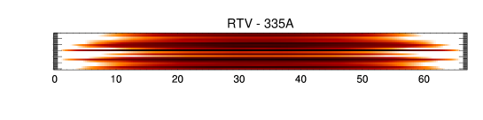
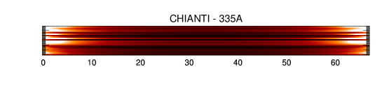
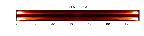
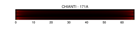
Figure 7: Synthetic (straightened) loop images obtained from collecting groups of 10 randomly heated strands, in SDO/AIA 335Å and 171Å channels, with models using RTV and CHIANTI radiative losses. The color scale is linear and exactly the same for a given channel (white is bright). The X-axis is measured in arcsec.

The faster cooling with CHIANTI losses below 2 MK has a second, important implication. The plasma in the strand spends a much longer time at temperatures well above 1-2 MK than below them. If a loop is made by a multitude of strands, each heated once randomly, most of the strands within a loop will have a high temperatures at any given time, while only few of them can be observed at temperatures at or below $\sim 1$ MK. This might explain, at least in part, why active regions have been found to be mostly covered by hot $\sim$3 MK loops with X-ray images and SDO/AIA 335Å channel images, and much less populated by warm $\sim$1 MK loops, like in the EUV 171Å channel in TRACE or SDO/AIA images, i.e. few loops are seen cooling from hot to warm status, much fewer than expected. To illustrate this effect, Figure 7 shows synthetic images of a multi-stranded loop in the two SDO channels obtained from the hydrodynamic simulations. We consider 200 straight strands grouped in bundles of 10 to mimic a limited instrument resolution. The straight aspect may recall a loop projected on the solar disk. Each strand has the evolution described above, but the start time of the heat pulse is shuffled: the strands brighten at random times. We take a snapshot in a regime situation, i.e. the emission spatially averaged over the stranded loop is equal to the average emission over the whole strand time evolution. We show images obtained both with RTV and CHIANTI radiative losses. The color scale is linear and chosen to be exactly the same in each channel. In the 335Å channel we see differences in the details but overall the loop appears to be bright. In the 171Å channel, there is a big qualitative change: the loop is much fainter, almost invisible, with the CHIANTI radiative losses. In a nutshell, the CHIANTI radiative losses significantly decrease the time that a given loop strand spends at a temperature between 1 and 3 MK, so that on the average it will be more difficult to observe loops in many narrow-band channels from AIA, TRACE, STEREO/EUVI and SOHO/EIT than expected when using RTV radiative losses. Since the onset of the accelerated (and then catastrophic) cooling depends on the plasma density, and hence on the rate of impulsive heating, changes in the radiative losses can have significant effects on heating rates determined from narrow-band images.

5 Discussion and conclusions

In this paper we have studied the effects of changes in the radiative loss curve on the evolution of an impulsively heated loop strand. Radiative losses can change due to 1) improvements in atomic models with the inclusion of more accurate atomic data and transition rates, or lines previously unavailable; 2) upgrades in the plasma ion abundance composition; 3) changes in the plasma element abundance composition. We have carried out our tests using two radiative loss curves, whose differences were due to all three these causes. The most recent curve, from CHIANTI version 7, had much more efficient radiative losses at temperatures in the 0.5-3 MK range than the older one (RTV losses). We expect similar effects also using other losses curves obtained from other spectral codes, with similar atomic models and element abundances (Sec.1). More efficient radiative losses may have effects on modeling other thermally unstable optically thin plasmas, such as flares, supernova remnants, accretion columns from circumstellar disks, novae, galactic cooling flows. Here we focus on their effects on the physics and structure of coronal loops, more in particular on the evolution of plasma confined inside a coronal magnetic flux tube and subject to a short and strong heat pulse.

The effect is very small in the initial phases of the evolution. Most previous studies of the flaring plasma focused on the rise and initial decay phase of the flare, and much less on the very late phases, so their results are not affected by changes in the radiative losses. On the contrary, Reale et al. (2012) studied the EUV late phase of a flare using the older RTV radiative losses, and were able to reproduce the observed light curves with success. The agreement they found between model and observations suggests two possibilities. First, a small change of model parameters may be enough to maintain the same degree of agreement if the CHIANTI radiative loss function is used: for example, increased radiative losses may require a smaller heating to lead to the final catastrophic cooling that explained the observations. Second, the element abundances in the flaring plasma may be lower than the coronal values assumed in the CHIANTI rates used in the present work so that the differences between the RTV and the CHIANTI radiative losses will be smaller.

Our results show that changes in the radiative loss curves have important effects on the late phases of a pulse-heated coronal loop strand, because they can change the cooling rate of the heated plasma and on the timing of the final catastrophic cooling. This can lead to immediate and interesting consequences on what we can expect from observations.

First, the change of cooling rate occurs at relatively low temperature ($\sim 2$ MK), and leads to considerable steepening of the cool side of the emission measure distribution. This change in EM(T) slope has important effects on our understanding of coronal plasma heating. In fact, earlier studies of pulse-heated loop models, using RTV-like radiative losses provided relatively flat EM(T) curves and such broad curves, not observed in active regions, have been invoked as an argument against the effectiveness of impulsive heating in non-flaring active regions (Warren et al., 2011). Thus, the change in slope caused by an improved radiative loss function can lead to a significant change of perspective.

Second, the temperature of the cooling plasma decreases more rapidly below 2 MK, and this might explain why we see very few loops cooling from X-rays to EUV bands in active regions.

Third, it is also interesting to notice that we do not expect faster cooling to occur in lower-regime loops: if the loop is heated by less intense pulses or in a more gradual and longer-lasting way, the plasma might never start a fast cooling. Whenever we observe 1 MK loops in UV “warm” channels this might provide an upper limit to the intensity and duration of the heat pulses that provide the energy.

Fourth, Reale et al. (2012) showed that a catastrophic cooling occurred at the end of the evolution of a post-flare loop, and explained the so-called EUV late phase observed by EVE during the decay of flares (Woods et al., 2011). Changes in radiative losses cause the predictions of the EUV late phase of flares to change considerably, and affect any estimate of flare impulsive heating rates made combining cooling loop models with observed EUV light curves.

This work uses one the latest release of an up-to-date spectral model. However, chances are that spectral codes will keep evolving and include many more lines and more accurate data as they become available. For example, there is evidence that we may still miss many important spectral lines (Testa et al., 2012) that can have significant effects on the radiative losses. As a consequence, we expect even more significant effects due to further spectral model improvements, so the present work can even be considered conservative to this respect. Also, element abundances are very important for radiative losses, so studies that provide better constraints on abundances are highly encouraged. On the contrary, effects of deviations from ionization equilibrium of the emitting species are negligible in the late phase of the flare, because the plasma is still at relatively high density, so that the ionization equilibrium times are quite short and the plasma is able to respond quickly and adapt to the rapid changes in the temperature (Reale et al., 2012).

In conclusion, in this work we report on the effect of upgrading the spectral models of optically thin emitting plasmas on modeling coronal plasma. In particular, we find that, while the increased emissivity obtained with new models has negligible effects on most of the plasma evolution predicted by models and in many plasma conditions, there is a very important implication for modeling of plasma confined in coronal loop strands heated by strong and fast energy pulses. Enhanced plasma emission in the 0.5-3 MK temperature range leads to faster cooling that might explain several pieces of evidence that questioned the validity of pulse-heated loop models. We point out that this kind of effects might be important also for modeling other thermally unstable optically thin plasmas, such as supernova remnants, accretion columns from circumstellar disks, novae.

We thank Peter Cargill for useful suggestions and the anonymous referee for constructive comments. Fabio Reale acknowledges support from Italian Ministero dell’Università e Ricerca and from Agenzia Spaziale Italiana (ASI), ASI/INAF agreement I/023/09/0. The work of Enrico Landi is supported by NASA grants NNX10AQ58G and NNX11AC20G, and by NSF grant AGS-1154443.

References

- Allen (1973) Allen, C. W. 1973, Astrophysical quantities (The Athlone Press, London)
- Antiochos et al. (1999) Antiochos, S., MacNeice, P., Spicer, D., & Klimchuk, J. 1999, Astrophys. J., 512, 985
- Antiochos (1980) Antiochos, S. K. 1980, ApJ, 241, 385
- Antiochos & Sturrock (1982) Antiochos, S. K. & Sturrock, P. A. 1982, ApJ, 254, 343
- Betta et al. (1997) Betta, R., Peres, G., Reale, F., & Serio, S. 1997, Astron. Astrophys. Suppl. Ser., 122, 585
- Betta et al. (2001) Betta, R., Peres, G., Reale, F., & Serio, S. 2001, Astron. Astrophys., 380, 341
- Bradshaw & Cargill (2005) Bradshaw, S. & Cargill, P. 2005, Astron. Astrophys., 437, 311
- Bradshaw & Cargill (2006) Bradshaw, S. & Cargill, P. 2006, Astron. Astrophys., 458, 987
- Bradshaw & Mason (2003) Bradshaw, S. & Mason, H. 2003, Astron. Astrophys., 407, 1127
- Bradshaw & Cargill (2010) Bradshaw, S. J. & Cargill, P. J. 2010, ApJ, 717, 163
- Cargill (1993) Cargill, P. 1993, Solar Phys., 147, 263
- Cargill (1994) Cargill, P. 1994, Astrophys. J., 422, 381
- Cargill (1995) Cargill, P. 1995, in Infrared tools for solar astrophysics: What’s next?, ed. J. . M.J.Penn, 17–+
- Cargill & Klimchuk (2004) Cargill, P. & Klimchuk, J. 2004, Astrophys. J., 605, 911
- Dere (2009) Dere, K. 2009, Astron. Astrophys., 497, 287
- Dere et al. (1997) Dere, K. P., Landi, E., Mason, H. E., Monsignori Fossi, B. C., & Young, P. R. 1997, A&AS, 125, 149
- Doschek et al. (1982) Doschek, G., Boris, J., Cheng, C., Mariska, J., & Oran, E. 1982, Astrophys. J., 258, 373
- Feldman (1992) Feldman, U. 1992, Phys. Scr, 46, 202
- Feldman et al. (1992) Feldman, U., Mandelbaum, P., Seely, J. F., Doschek, G. A., & Gursky, H. 1992, ApJS, 81, 387
- Field (1965) Field, G. B. 1965, ApJ, 142, 531
- Foster et al. (2012) Foster, A., Ji, L., Smith, R., & Brickhouse, N. 2012, ApJ
- Gan et al. (1991) Gan, W., Zhang, H., & Fang, C. 1991, Astron. Astrophys., 241, 618
- Guarrasi et al. (2010) Guarrasi, M., Reale, F., & Peres, G. 2010, ApJ, 719, 576
- Hansteen (1993) Hansteen, V. 1993, Astrophys. J., 402, 741
- Kaastra et al. (1996) Kaastra, J. S., Mewe, R., Liedahl, D. A., et al. 1996, A&A, 314, 547
- Klimchuk (2006) Klimchuk, J. 2006, Solar Phys., 234, 41
- Klimchuk et al. (2008) Klimchuk, J., Patsourakos, S., & Cargill, P. 2008, Astrophys. J., 682, 1351
- Landi et al. (2012) Landi, E., Del Zanna, G., Young, P. R., Dere, K. P., & Mason, H. E. 2012, ApJ, 744, 99
- Landi & Landini (1999) Landi, E. & Landini, M. 1999, A&A, 347, 401
- Landini & Monsignori Fossi (1970) Landini, M. & Monsignori Fossi, B. C. 1970, A&A, 6, 468
- MacNeice (1986) MacNeice, P. 1986, Solar Phys., 103, 47
- McClymont & Canfield (1983) McClymont, A. N. & Canfield, R. C. 1983, ApJ, 265, 497
- Müller et al. (2003) Müller, D., Hansteen, V., & Peter, H. 2003, Astron. Astrophys., 411, 605
- Nagai (1980) Nagai, F. 1980, Solar Phys., 68, 351
- Nagai & Emslie (1984) Nagai, F. & Emslie, A. 1984, Astrophys. J., 279, 896
- Parker (1988) Parker, E. 1988, Astrophys. J., 330, 474
- Parker (1953) Parker, E. N. 1953, ApJ, 117, 431
- Patsourakos & Klimchuk (2005) Patsourakos, S. & Klimchuk, J. 2005, Astrophys. J., 628, 1023
- Peres et al. (2000) Peres, G., Orlando, S., Reale, F., Rosner, R., & Hudson, H. 2000, Astrophys. J., 528, 537
- Peres et al. (1993) Peres, G., Reale, F., & Serio, S. 1993, in Astrophysics and Space Science Library, Vol. 183, Physics of Solar and Stellar Coronae: G.S. Vaiana Memorial Symposuim, ed. J. Linsky & S. Serio (Dordrecht; Boston: Kluwer), 151
- Peres et al. (1987) Peres, G., Reale, F., Serio, S., & Pallavicini, R. 1987, ApJ, 312, 895
- Peres et al. (1982) Peres, G., Serio, S., Vaiana, G., & Rosner, R. 1982, Astrophys. J., 252, 791
- Raymond & Smith (1977) Raymond, J. C. & Smith, B. W. 1977, ApJS, 35, 419
- Reale (2007) Reale, F. 2007, Astron. Astrophys., 471, 271
- Reale (2010) Reale, F. 2010, Living Reviews in Solar Physics, 7, 5
- Reale et al. (2011) Reale, F., Guarrasi, M., Testa, P., et al. 2011, ApJ, 736, L16
- Reale et al. (2012) Reale, F., Landi, E., & Orlando, S. 2012, ApJ, 746, 18
- Reale & Orlando (2008) Reale, F. & Orlando, S. 2008, Astrophys. J., 684, 715
- Reale et al. (2000) Reale, F., Peres, G., Serio, S., et al. 2000, Astrophys. J., 535, 423
- Rosner et al. (1978) Rosner, R., Tucker, W., & Vaiana, G. 1978, Astrophys. J., 220, 643
- Soler et al. (2012) Soler, R., Ballester, J. L., & Parenti, S. 2012, A&A, 540, A7
- Terzo et al. (2011) Terzo, S., Reale, F., Miceli, M., et al. 2011, ApJ, 736, 111
- Testa et al. (2012) Testa, P., Drake, J. J., & Landi, E. 2012, ApJ, 745, 111
- Testa et al. (2011) Testa, P., Reale, F., Landi, E., DeLuca, E. E., & Kashyap, V. 2011, ApJ, 728, 30
- Tucker & Gould (1966) Tucker, W. H. & Gould, R. J. 1966, ApJ, 144, 244
- Tucker & Koren (1971) Tucker, W. H. & Koren, M. 1971, ApJ, 168, 283
- Vernazza et al. (1981) Vernazza, J., Avrett, E., & Loeser, R. 1981, Astrophys. J. Suppl. Ser., 45, 635
- Viall & Klimchuk (2011) Viall, N. M. & Klimchuk, J. A. 2011, ApJ, 738, 24
- Warren et al. (2002) Warren, H., Winebarger, A., & Hamilton, P. 2002, Astrophys. J. Lett., 579, L41
- Warren et al. (2003) Warren, H., Winebarger, A., & Mariska, J. 2003, Astrophys. J., 593, 1174
- Warren et al. (2011) Warren, H. P., Brooks, D. H., & Winebarger, A. R. 2011, ApJ, 734, 90
- Woods et al. (2011) Woods, T. N., Hock, R., Eparvier, F., et al. 2011, ApJ, 739, 59