Earth rotation prevents exact solid body rotation of fluids in the laboratory

Abstract

We report direct evidence of a secondary flow excited by the Earth rotation in a water-filled spherical container spinning at constant rotation rate. This so-called tilt-over flow essentially consists in a rotation around an axis which is slightly tilted with respect to the rotation axis of the sphere. In the astrophysical context, it corresponds to the flow in the liquid cores of planets forced by precession of the planet rotation axis, and it has been proposed to contribute to the generation of planetary magnetic fields. We detect this weak secondary flow using a particle image velocimetry system mounted in the rotating frame. This secondary flow consists in a weak rotation, thousand times smaller than the sphere rotation, around a horizontal axis which is stationary in the laboratory frame. Its amplitude and orientation are in quantitative agreement with the theory of the tilt-over flow excited by precession. These results show that setting a fluid in a perfect solid body rotation in a laboratory experiment is impossible — unless tilting the rotation axis of the experiment parallel to the Earth rotation axis.

1 Introduction

There are few examples of fluid mechanics experiments at the laboratory scale in which the Earth’s Coriolis force has a measurable influence. Such experiments may be considered as fluid analogues to the Foucault pendulum. The most popular instance is certainly the drain of a bathtube vortex [1]. Although this is the subject of common misconception, it is actually possible to detect the influence of the Earth’s rotation on the vortex, but only under extremely careful experimental conditions, far from the everyday experience [2]. Thermal convection is another example, in which a slow drift of the large-scale flow due to the Earth rotation has been detected in very controlled systems [3, 4].

In this letter we describe an experiment which may be considered as the most simple fluid Foucault pendulum: it consists in a volume of water enclosed in a spherical container spinning at constant rotation rate $\Omega_{0}$ (fig. 1). After a transient known as spin-up, the water is expected to rotate as a solid body at the same rate $\Omega_{0}$ [5]. The timescale for this spin-up is classically given by the Ekman time $\tau_{E}=R\,(\nu\Omega_{0})^{-1/2}$, where $R$ is the radius of the sphere and $\nu$ the kinematic viscosity of the fluid. For a typical laboratory experiment using water, this timescale is usually of order of a minute, so after a few tens of minutes a perfect solid-body rotation should be reached, with the fluid exactly at rest in the frame of the container. If this simple experiment is performed on Earth, it is expected that the Earth rotation could prevent from reaching this idealized solid rotation state [6, 7]. A weak secondary flow, known as tilt-over flow [5, 8, 9], is induced by the precession of the rotation vector ${\bf\Omega}_{0}$ of the container by the Earth rotation vector ${\bf\Omega}_{p}$. Seen from the laboratory frame of reference, the fluid particles rotating at velocity ${\bf u}_{0}={\bf\Omega}_{0}\times{\bf r}$ experience a Coriolis force per unit mass ${\bf f}_{c}=-2{\bf\Omega}_{p}\times{\bf u}_{0}$. This Coriolis force disturbs the fluid particles periodically at frequency $\Omega_{0}$, and tends to deflect their trajectory towards the plane normal to ${\bf\Omega}_{p}$.

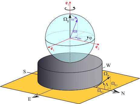
Figure 1: (Color online) Sketch of the rotating platform and the water filled sphere. $({\bf e}_{1},{\bf e}_{2},{\bf e}_{3})$ is a Cartesian coordinates system attached to the laboratory frame. The platform is rotating at ${\bf\Omega}_{0}=\Omega_{0}\,{\bf e}_{3}$ in the laboratory. ${\bf\Omega}_{p}$ is the Earth rotation vector at the latitude $\Lambda=48.70$^o  of the laboratory. ${\boldsymbol{\omega}}$ is the rotation vector of the tilt-over flow in the bulk. The rotation vectors are not to scale.

Precession driven flows in spherical or spheroidal containers and in spheroidal shells have received considerable interest since Poincaré [10], because of their importance to geophysical and astrophysical flows [8, 9]. In the case of the Earth, rotating with a period $T_{0}\sim 1$ day, the precession of its rotation axis, at a period $T_{p}\simeq 26~{}000$ years, could produce large excursions of the rotation axis of the liquid core [11]. Precession driven flows have also been proposed by Malkus [9] to contribute to the generation of planetary magnetic fields, which has been later confirmed by Kerswell [12] and Tilgner [13]. Kida [14] recently proposed a complete solution for the flow in a rapidly rotating sphere under weak precession, including a detailed analysis of the conical shear layers detached from the critical latitudes.

First evidence of a tilt-over flow excited by the Earth rotation in a laboratory experiment has been reported by Vanyo and Dunn [6], using visualizations by dyes and buoyant tracers, but without quantitative determination of the tilt-over flow properties. Recently, Triana et al.[7] obtained indirect evidence of this effect, from one-dimensional velocity profiles in a rotating water-filled spherical shell, 3 m in diameter, containing an inner co-rotating sphere. However, no quantitative agreement with the theory of Busse [8] could be obtained in their experiment.

Based on the same idea, we provide in this letter, by means of particle image velocimetry measurements (PIV), the first direct visualization of the precession flow driven by the Earth rotation in a sphere rotating in the laboratory. These measurements are a technical challenge, because of weakness of the velocity signal of this tilt-over flow (the fluid rotation axis is tilted by less than 0.2^o  with respect to the sphere rotation axis). A quantitative agreement with the theory of Busse is demonstrated, both for the magnitude and the orientation of the secondary circulation.

2 Physical origin of the tilt-over flow

Poincaré [10] first analyzed the precession flow in a sphere in the singular case of a perfect fluid. He showed that the inviscid solution consists in a solid-body rotation around an axis parallel to $\bf{\Omega}_{p}$, but of undefined amplitude. In the presence of weak viscosity, far from the boundaries, the tilt-over flow may still be described as a solid-body rotation, with a rotation vector ${\boldsymbol{\omega}}$ tilted with respect to ${\bf\Omega}_{0}$, and stationary in the precessing frame (the laboratory frame here). We note in the following ${\boldsymbol{\omega}^{\prime}}={\boldsymbol{\omega}}-{\bf\Omega_{0}}$ the rotation vector of the fluid in the bulk measured in the rotating frame.

Remarkably, the presence of viscosity, even weak, drastically changes the rotation vector of the fluid ${\boldsymbol{\omega}}$ compared to the inviscid solution of Poincaré. The orientation and amplitude of ${\boldsymbol{\omega}}$ for a viscous fluid are now non trivial functions of the Poincaré number $\Omega_{p}/\Omega_{0}$ and of the Ekman number $E=\nu/(\Omega_{0}R^{2})$. In the limit $\Omega_{p}/\Omega_{0}\ll\sqrt{E}\ll 1$, the rotation vector ${\boldsymbol{\omega}}$ is almost equal to ${\bf\Omega}_{0}$, and the small correction ${\boldsymbol{\omega}^{\prime}}$ is almost normal to ${\bf\Omega}_{0}$. This tilt-over flow has been described by Busse [8] as one among a dense family of inertial modes, of eigenfrequency given by $\Omega_{0}$ (see Ref. [5] for a general description of inertial modes in a sphere). When forced by precession, the magnitude $\omega^{\prime}$ of this tilt-over flow can be determined by a simple balance between the Coriolis torque (in the bulk) and the viscous torque (at the surface of the container). The Coriolis torque is of order $\Gamma_{c}\sim\rho R^{4}f_{c}\sim\rho R^{5}\Omega_{p}\Omega_{0}\cos\Lambda$, with $\rho$ the fluid density and $\cos\Lambda=|{\bf\Omega}_{0}\times{\bf\Omega}_{p}|/\Omega_{0}\Omega_{p}$. The viscous stress is given by $\sigma\sim\rho\nu\Delta u/\delta$, where $\Delta u\simeq\omega^{\prime}R$ is the small velocity jump between the container wall and the fluid bulk, and $\delta=(\nu/\Omega_{0})^{1/2}$ is the thickness of the Ekman boundary layer. The resulting viscous torque is of order $\Gamma_{\nu}\sim R^{3}\sigma\sim\rho\nu\omega^{\prime}R^{4}/\delta$. Balancing the two torques gives the simple relation

$$\omega^{\prime}\sim E^{-1/2}\Omega_{p}\cos\Lambda.$$ (1)

Although very weak, this tilt-over correction may be significantly larger than the Earth rotation rate in a typical laboratory experiment where $E\ll 1$.

3 Experimental Setup

The experimental setup, sketched in fig. 1, consists in a spherical glass tank, of inner radius $R=115\pm 0.25$ mm, filled with water and mounted on the center of a precision rotating turntable of $2$ m in diameter. We use two Cartesian coordinate systems, both with origin at the center of the sphere: (i) $({\bf e}_{1},{\bf e}_{2},{\bf e}_{3})$, attached to the laboratory reference frame (fig. 1), with ${\bf e}_{1}$ pointing to East, ${\bf e}_{2}$ pointing to North and ${\bf e}_{3}$ along the vertical; (ii) $({\bf e}_{x},{\bf e}_{y},{\bf e}_{z})$, attached to the rotating platform (fig. 2), with ${\bf e}_{z}={\bf e}_{3}$, in which the measurements are performed.

The platform is rotating in the laboratory frame with a rotation vector ${\bf\Omega}_{0}=\Omega_{0}\,{\bf e}_{3}$. The angular velocity $\Omega_{0}$ is varied between 2 and 16 rpm, with temporal fluctuations less than $\pm 5\times 10^{-4}$. The Ekman number $E=\nu/(\Omega_{0}R^{2})$ varies between $3.6\times 10^{-4}$ and $4.6\times 10^{-5}$ in this range of $\Omega_{0}$. In fig. 1, the rotation vector of the Earth ${\bf\Omega_{p}}$ is also shown, for the latitude $\Lambda=48.70$^o of our laboratory in Orsay. The relative scale of the vectors ${\bf\Omega_{0}}$ and ${\bf\Omega_{p}}$ is obviously not realistic in this figure: the Earth rotation rate is $\Omega_{p}\simeq 6.9\times 10^{-4}$ rpm $\sim 2\pi/(\mbox{1 day})$, which yields a Poincaré number $\Omega_{p}/\Omega_{0}$ ranging from $3.5\times 10^{-4}$ to $4.3\times 10^{-5}$.

After the start of the platform rotation, we wait at least $\tau_{w}=2$ hours before data acquisition in order to reach a stationary regime. This waiting time represents at least $30\,\tau_{E}$, where $\tau_{E}=R\,(\nu\Omega_{0})^{-1/2}$ is the Ekman spin-up time. This indicates that the solid-body rotation state should be reached, apart from precession effects, with a relative precision better than $\exp(-\tau_{w}/\tau_{E})\simeq 10^{-13}$.

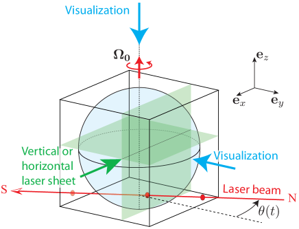
Figure 2: (Color online) Schematic view of the cubic water tank containing the 115 mm radius glass sphere, mounted together on the rotating platform. PIV measurements are achieved in off-centered vertical and horizontal planes, located at $y_{\rm mes}=+22$ mm and $z_{\rm mes}=+22$ mm, using a corotating laser sheet and a camera aiming normally at it. The angle $\theta(t)$ between the images and the North direction is determined using a continuous laser beam aligned along the North-South orientation and crossing the rotation axis.

Velocity fields are measured in the rotating frame using a two-dimensional PIV system [15] mounted on the rotating platform, in either a vertical $({\bf e}_{x},{\bf e}_{z})$ or a horizontal $({\bf e}_{x},{\bf e}_{y})$ plane (fig. 2). These measurement planes are off-centered, at $y_{\rm mes}/R=z_{\rm mes}/R\simeq 0.19$ (see fig. 2), in order to get better insight in the spatial structure of the flow. Optical distortions are reduced by immersing the glass sphere in a square glass tank of 300 mm side also filled with water. The distortion is found less than 5% for $r<0.9R$. The fluid is seeded with $10$ $\mu$m tracer particles, and illuminated by a corotating laser sheet generated by a $140$ mJ Nd:YAG pulsed laser. For both horizontal and vertical measurements, the sphere cross-section is imaged with a high resolution $2048\times 2048$ pixels camera aiming normally at the laser sheet.

For each rotation rate $\Omega_{0}$, a set of 2 000 images is acquired, covering at least 80 rotation periods. The sampling rate is synchronized with the platform rotation rate, with a number of images per rotation ranging from 24 (for low $\Omega_{0}$) to 9 (for large $\Omega_{0}$). PIV fields are computed over successive images using $32\times 32$ pixels interrogation windows with $50\%$ overlap, leading to a spatial resolution of about $2$ mm. This resolution is not enough to resolve the thickness of the Ekman boundary layers, $\delta\simeq R\,E^{1/2}=0.8-2.2$ mm, but is appropriate for the large scales of the precession flow expected in the bulk.

In view of the very low velocity expected for the precession flow, the resolution of the velocity measurement is critical in our experiment. The characteristic velocities of the flow encountered in this work ranges from $0.01$ to $0.4$ mm s^-1 for $\Omega_{0}$ between $2$ and $16$ rpm. For the sampling rates considered here, these velocities correspond to a typical frame-by-frame particle displacement of 0.16 to 2.6 pixels only. Although very weak, such displacement may actually be measured using PIV with sub-pixel interpolation of the correlation peak. For interrogation windows of size $32\times 32$ pixels, an accuracy of 0.05 pixel can be achieved using this technique [16, 15], yielding a signal-to-noise ratio ranging from 3 (low $\Omega_{0}$) to 50 (large $\Omega_{0}$).

The orientation of the experiment with respect to the Earth rotation axis is monitored using a continuous laser beam aligned along the North-South direction and passing through the rotation axis of the sphere (see fig. 2). The beam crosses the cubic glass tank and is therefore visible on the recorded images. The angle $\theta(t)$ between the South-North direction and the measurement fields (see fig. 2) can be determined for each image with a precision better than $\pm 0.5$^o.

4 Structure of the tilt-over flow

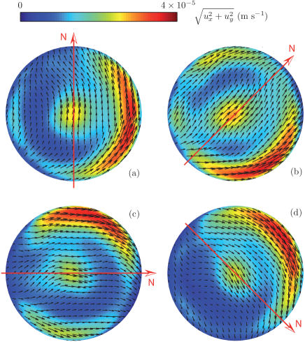
Figure 3: Horizontal velocity fields measured in the rotating frame, in the off-centered horizontal plane at $z_{\rm mes}/R\simeq 0.19$ for $\Omega_{0}=6$ rpm ($E=1.2\times 10^{-4}$), with a phase shift of $\pi/4$ between each image. The platform rotation is anticlockwise. The red arrows indicate the direction of the North at each time. Resolution of the velocity fields has been reduced by a factor 5 for better visibility.

We first show in fig. 3 the flow measured in the horizontal plane in the rotating frame for a rotation rate $\Omega_{0}=6$ rpm. This flow represents the departure between the total flow in the laboratory frame and the solid body rotation at $\Omega_{0}$. In order to improve the quality of the velocity fields shown here, a phase average is performed over the velocity fields at the platform rotation rate $\Omega_{0}$. This procedure allows to decrease the broad-band PIV measurement noise by a factor $N^{1/2}$, where $N$ is the number of recorded rotation periods ($N\geq 80$). The spatial structure of the precession flow can finally be extracted with a signal-to-noise ratio of at least 30 for all rotations rates.

The four snapshots shown in fig. 3 are separated by a phase shift of $\pi/4$, with a phase origin chosen such that ${\bf e}_{x}={\bf e}_{1}$ (i.e. ${\bf e}_{y}$ pointing to the North). In spite of the very weak velocity signal (of order of 0.04 mm s^-1, to be compared to the typical velocity of the sphere boundaries, $\Omega_{0}\,R\simeq 72$ mm s^-1), we clearly observe a well-defined flow pattern, which is rotating as a whole at the platform rotation rate but in the opposite direction. This weak flow is therefore stationary in the laboratory frame. Assuming that the total flow in the laboratory frame is a solid body rotation of vector ${\boldsymbol{\omega}}$ slightly tilted with respect to ${\bf\Omega}_{0}$, the measured flow must be a solid body rotation of rotation vector ${\boldsymbol{\omega}^{\prime}}={\boldsymbol{\omega}}-{\bf\Omega}_{0}$. Since the measurement plane is shifted at $z_{\rm mes}/R\simeq 0.19$, the resulting horizontal velocity field must be uniform in the bulk, given by ${\boldsymbol{\omega}^{\prime}}\times(z_{\rm mes}{\bf e}_{3})$, and rotating in the anticyclonic direction at frequency $\Omega_{0}$, which is precisely what we observe. Snapshots at other values of $\Omega_{0}$ show essentially the same flow patterns.

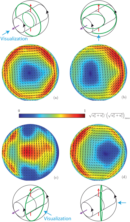
Figure 4: Vertical velocity fields measured in the rotating frame, in the off-centered vertical plane at $y_{\rm mes}/R\simeq 0.19$ for $\Omega_{0}=6$ rpm ($E=1.2\times 10^{-4}$), with a phase shift of $\pi/4$ between each image. The color maps the vertical velocity norm normalized by its maximum in each field. The phase origin is not the same as in fig. 3.

Measurements in the vertical plane, shown in fig. 4, confirm this flow structure. In this configuration, the camera is now rotating around the vortex of quasi-horizontal rotation vector ${\boldsymbol{\omega}^{\prime}}$ stationary in the laboratory frame. The 4 snapshots taken over half a rotation around the vortex actually show the following sequence: (a) anticlockwise, with ${\boldsymbol{\omega}^{\prime}}$ pointing towards the camera; (b) intermediate; (c) ascending, with ${\boldsymbol{\omega}^{\prime}}$ pointing to the left; (d) intermediate. If the tilt-over flow were a pure solid-body rotation, the ascending flow in the snapshot (c) would be uniform, given by ${\boldsymbol{\omega}^{\prime}}\times({y_{\rm mes}{\bf e}_{y})}$, which is approximately the case far from the boundaries. The wall region where the flow departs from a pure uniform flow has a thickness of order of $0.3\,R$, which is much larger than the expected Ekman thickness $E^{1/2}R\simeq 0.01\,R$. The tilt-over flow is therefore not exactly a pure solid body rotation, in agreement with numerical results obtained in a spherical shell with a very small stress-free inner solid core [17]. Indeed, because of the breakdown of the Ekman layer at the so-called critical circles, a pure solid body rotation cannot be a uniformly valid solution [14].

5 Viscous prediction for the tilt-over flow forced by precession

We compute here the rotation vector ${\boldsymbol{\omega}}$ in the bulk of the fluid viewed from the precessing frame of reference (here the laboratory frame), following Refs. [18, 19]. The differential rotation between the fluid in the bulk rotating at ${\boldsymbol{\omega}}$ and the sphere boundary rotating at ${\bf\Omega}_{0}$ is matched across an Ekman boundary layer of typical thickness $RE^{1/2}$. We therefore assume $E\ll 1$, such that a separation between a bulk flow and a thin boundary layer may be assumed. In the steady state, the viscous torque ${\bf\Gamma}_{\nu}$ exerted by the boundary layers on the fluid in the bulk is balanced by the Coriolis torque ${\bf\Gamma}_{c}$ (note that the pressure torque is zero here because of spherical symmetry). This balance, projected along $\boldsymbol{\omega}$ and along the two directions normal to $\boldsymbol{\omega}$, yields the following nonlinear system of equations [5, 19],

$$\omega_{1}^{2}+\omega_{2}^{2} =\omega_{3}(\Omega_{0}-\omega_{3}),$$ (2)

$$\frac{\Omega_{p}}{\sqrt{E}}\left(\omega_{3}\cos\Lambda-\omega_{2}\sin\Lambda\right) =\ldots$$

$$\lambda_{r}\omega_{1}\omega_{3}^{1/4}\Omega_{0}^{3/4}+\lambda_{i}\omega_{2}\frac{\Omega_{0}^{5/4}}{\omega_{3}^{1/4}},$$ (3)

$$\frac{\Omega_{p}}{\sqrt{E}}\omega_{1}\cos\Lambda =\lambda_{r}\Omega_{0}^{3/4}\omega_{3}^{1/4}(\Omega_{0}-\omega_{3}),$$ (4)

where $\lambda_{r}$ and $\lambda_{i}$ are respectively the non-dimensional viscous damping rate and viscous correction to the eigenfrequency of the tilt-over mode. Their values have been obtained by Greenspan [5] and completed by Zhang et al.[20], $\lambda_{r}=-2.62$ and $\lambda_{i}=0.258$. In presence of viscosity, the eigenfrequency $\Omega_{0}$ of the inviscid tilt-over mode becomes $\Omega_{0}+(\lambda_{i}+\textrm{i}\lambda_{r})\sqrt{E}\sqrt{\Omega_{0}\,\omega}$ [18, 20], which means that, if the precession forcing is switched off, the tilt-over mode starts to rotate in the inertial frame at a frequency $\lambda_{i}\sqrt{E}\sqrt{\Omega_{0}\,\omega}$, while exponentially decaying at a rate $|\lambda_{r}|\sqrt{E}\sqrt{\Omega_{0}\,\omega}$.

Equation (2) reflects the fact the work done per unit time by the viscous torque is zero, ${\bf\Gamma}_{\nu}\cdot{\boldsymbol{\omega}}=0$, since the work done by the Coriolis force is zero by definition. This equation, which can be recast into ${\boldsymbol{\omega}}\cdot({\boldsymbol{\omega}}-{\bf\Omega_{0}})=0$, simply expresses the so-called “no spin-up” condition, indicating that there is no differential rotation between the fluid and the sphere in the direction of the fluid rotation. This right angle between ${\boldsymbol{\omega}}$ and ${\boldsymbol{\omega}^{\prime}}={\boldsymbol{\omega}}-{\bf\Omega}_{0}$ indicates that the rotation rate $|{\boldsymbol{\omega}}|$ of the fluid is lower than $\Omega_{0}$.

If we further assume that the Poincaré number $\Omega_{p}/\Omega_{0}$ is small compared to $E^{1/2}$, the rotation vector ${\boldsymbol{\omega}}$ is almost aligned with ${\bf\Omega_{0}}$, and the system of equation (2)-(4) can be simplified. More precisely, this regime applies for rotation rates $\Omega_{0}\gg\Omega_{0,c}$, with

$$\Omega_{0,c}=\left(\frac{\Omega_{p}R\sin\Lambda}{\lambda_{r}\sqrt{\nu}}\right)^{2}.$$ (5)

This condition is comfortably satisfied in the present experiments, with $\Omega_{0,c}\simeq 5.2\times 10^{-5}$ rpm. In this limit, the components of the tilt-over flow can be explicitly derived,

$$\omega_{1} \simeq \frac{\Omega_{p}\cos\Lambda}{\lambda_{r}}\left(\frac{\Omega_{0}R^{2}}{\nu}\right)^{1/2},$$ (6)

$$\omega_{2} \simeq \frac{\lambda_{i}}{\lambda_{r}}\omega_{1},$$ (7)

$$\omega_{3} \simeq \Omega_{0}.$$ (8)

The horizontal projection of ${\boldsymbol{\omega}}$ in the laboratory frame, ${\boldsymbol{\omega}}_{h}=\omega_{1}{\bf e}_{1}+\omega_{2}{\bf e}_{2}$, has therefore an amplitude

$$\omega_{h}=\frac{\Omega_{p}\cos\Lambda}{|\lambda_{r}|}\left(\frac{\Omega_{0}R^{2}}{\nu}\right)^{1/2}\left(1+\frac{\lambda_{i}^{2}}{\lambda_{r}^{2}}\right)^{1/2},$$ (9)

which has indeed the expected form (1). Note that, in the limit considered here ($\Omega_{p}/\Omega_{0}\ll\sqrt{E}$), the horizontal projection ${\boldsymbol{\omega}}_{h}$ measured in the experiment almost coincides with ${\boldsymbol{\omega}^{\prime}}$.

In this limit, the angle $\varphi$ between ${\boldsymbol{\omega}}_{h}$ and ${\bf e}_{1}$ (the East direction) is constant, and given by

$$\varphi=\arctan\left(\frac{\omega_{2}}{\omega_{1}}\right)=\arctan\frac{\lambda_{i}}{\lambda_{r}}=174.35^{\mathrm{o}},$$ (10)

showing that ${\boldsymbol{\omega}}_{h}$ points almost to the West (along $-{\bf e}_{1}$), with a slight component to the North. Remarkably, this asymptotic angle obtained in the limit of large $\Omega_{0}$ is almost perpendicular to the inviscid prediction of Poincaré, for which ${\boldsymbol{\omega}}_{h}$ points to the North (i.e. $\varphi=90$^o). This indicates that, even for very low viscosity, the boundary layers have a critical influence on the tilt-over flow, provided that $\Omega_{p}/\Omega_{0}\ll E^{1/2}$.

6 Comparison with the experimental tilt-over flow

The rotation rate $\omega_{h}$ of the tilt-over flow and its angle $\varphi$ with the East have been systematically determined for $\Omega_{0}$ ranging from 2 to 16 rpm. These data have been extracted independently from the raw velocity fields measured in the vertical and horizontal planes, and are compared here with the theoretical predictions (9)-(10) in figs. 5 and 6.

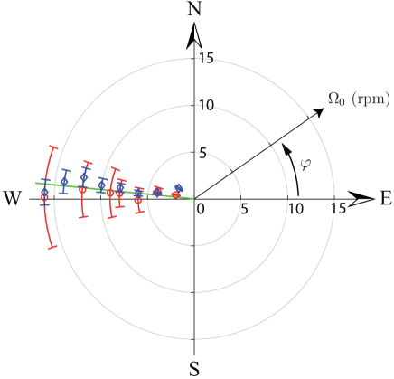
Figure 5: (Color online) Angle $\varphi$ between the rotation vector of the tilt-over flow and ${\bf e}_{1}$ (i.e. East) as a function of the rotation rate $\Omega_{0}$ in polar coordinates. Measurements are obtained in the horizontal ($\circ$) and the vertical ($\diamond$) plane respectively. The continuous line shows the theoretical prediction $\varphi=174.35^{\mathrm{o}}$ (10).

Measurements of the vortex angle $\varphi$ from the PIV data in the vertical plane have been obtained as follows: the horizontal vorticity, spatially averaged over a central region of 50 mm radius, shows a harmonic oscillation at frequency $\Omega_{0}$. At each period, the delay between the time $t_{\rm max}$ of maximum vorticity (when ${\boldsymbol{\omega}}_{h}$ points to the camera) and the time at which the North-South laser beam is aligned with the camera axis is computed. Knowing the instantaneous angle $\theta(t)$ between the camera incidence and the South-North direction, we can simply deduce the angle of the vortex as $\varphi=\theta(t_{\rm max})+90$^o. An independent estimate for $\varphi$ has been determined from the data in the horizontal plane, by computing the time averaged (and spatially averaged over the region $|{\bf r}|<50$ mm) angle of the velocity with respect to the East direction ${\bf e}_{1}$.

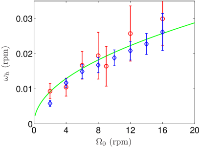
Figure 6: Horizontal rotation rate $\omega_{h}$ of the tilt-over flow as a function of the rotation rate of the platform $\Omega_{0}$, measured in the horizontal ($\circ$) and vertical ($\diamond$) planes. The continuous line shows the prediction (9).

The rotation rate $\omega_{h}$ of the horizontal component of the tilt-over flow has been determined from the vertical cuts as half the spatially averaged (over a central disk of radius 50 mm) vorticity, measured at the times $t_{\rm max}$ of maximum vorticity. $\omega_{h}$ has also been determined independently from the horizontal cuts, as $\omega_{h}=\langle|{\bf u}_{h}|\rangle/z_{\rm mes}$, where $\langle\cdot\rangle$ is an average over time and over the region $|{\bf r}|<50$ mm, and $z_{\rm mes}$ is the height of the measurement plane.

For both measurements in the horizontal and vertical planes, one value of $\varphi$ and $\omega_{h}$ is obtained at each rotation period. From this set, the average and standard deviation are computed over the 80 periods recorded for each rotation rate. In addition to the temporal fluctuations, the errorbars in figs. 5 and 6 also include the variations of $\varphi$ and $\omega_{h}$ when varying the radius of the averaging region between $25$ and $75$ mm. For both quantities, the estimates determined from the two measurement planes closely agree, although data from the horizontal plane systematically show a larger scatter.

The vortex angle measured from both vertical and horizontal planes, $\varphi\simeq 173\pm 4$^o  and $175\pm 11$^o respectively (fig. 5), are in good agreement with the theoretical prediction (10) . Similarly, the rotation rate $\omega_{h}$ measured in both planes closely follow the prediction (9) to within 20% over the range $\Omega_{0}=2-16$ rpm (fig. 6). The agreement of $\omega_{h}$ and $\varphi$ with the theoretical predictions is remarkable in view of the very weak velocity signal, providing strong evidence that the weak secondary flow that we observe originates from the precession of the experiment by the Earth rotation. The magnitude of the secondary rotation lies in the range $(1.5-3)\times 10^{-3}\,\Omega_{0}$, confirming that the rotation vector ${\boldsymbol{\omega}}$ of the fluid is almost aligned with ${\bf\Omega}_{0}$, with a very weak angular departure of $\omega_{h}/\Omega_{0}<0.2$^o.

7 Conclusion

Measuring the influence of the Earth rotation at the laboratory scale is a technical challenge. In the fluid analogue of the Foucault pendulum presented in this letter, the very weak precession driven flow would have been impossible to detect directly from the laboratory frame. Probing the flow in the rotating frame naturally subtracts the first-order rotation and allows us to detect this slight correction. We note that such residual tilt-over flow forced by the Earth rotation defines an irreducible background flow which should be present in every rotating fluid experiments, routinely used as models for geophysical and astrophysical flows in the laboratory.

- [1] Perrot M., C. R. Acad. Science, XLIX (1859) 637.
- [2] Shapiro A.H., Nature, 196 (1962) 1080.
- [3] Pantaloni J., Cerisier P., Bailleux R. and Gerbaud C., J. Physique Lettres, 42 (1981) L147.
- [4] Brown E. and Ahlers G., Phys. Fluids, 18 (2006) 125108.
- [5] Greenspan H., The theory of rotating fluids (Cambridge University Press, London) 1968.
- [6] Vanyo J.P. and Dunn J.R., Geophys. J. Int., 142 (2000) 409.
- [7] Triana S.A., Zimmerman D.S. and Lathrop D.P., J. Geophys. Res., 117 (2012), B04103.
- [8] Busse F.H., J. Fluid Mech., 33 (1968) 739.
- [9] Malkus W.V.R., Science, 160 (1968) 259.
- [10] Poincaré R., Bull. Astron., 27 (1910) 321.
- [11] Greff-Lefftz M. and Legros H., Science, 286 (1999) 1707.
- [12] Kerswell R.R., J. Fluid Mech., 321 (1996) 335.
- [13] Tilgner A., Phys. Fluids, 17 (2005) 034104.
- [14] Kida S., J. Fluid Mech., 680 (2011) 150.
- [15] DaVis, LaVision GmbH, complemented by the PIVMat toolbox for Matlab, http://www.fast.u-psud.fr/pivmat.
- [16] Raffel M., Willert C., Wereley S. and Kompenhans J., Particle Image Velocimetry (Spring-Verlag, Berlin) 2007.
- [17] Tilgner A. and Busse F.H., J. Fluid Mech., 426 (2001) 387.
- [18] Noir J., Cardin P., Jault D. and Masson J.-P., Geophys. J. Int., 154 (2003) 407.
- [19] Cébron D., Le Bars M. and Meunier P., Phys. Fluids, 22 (2010) 101063.
- [20] Zhang K., Liao X. and Earnshaw P., J. Fluid Mech., 504 (2004) 1.