Universal Algorithm for Online Trading Based on the Method of Calibration

Abstract

We present a universal method for algorithmic trading in Stock Market which performs asymptotically at least as well as any stationary trading strategy that computes the investment at each step using a fixed function of the side information that belongs to a given RKHS (Reproducing Kernel Hilbert Space). Using a universal kernel, we extend this result for any continuous stationary strategy. In this learning process, a trader rationally chooses his gambles using predictions made by a randomized well-calibrated algorithm. Our strategy is based on Dawid’s notion of calibration with more general checking rules and on some modification of Kakade and Foster’s randomized rounding algorithm for computing the well-calibrated forecasts. We combine the method of randomized calibration with Vovk’s method of defensive forecasting in RKHS. Unlike in statistical theory, no stochastic assumptions are made about the stock prices. Our empirical results on historical markets provide strong evidence that this type of technical trading can “beat the market” if transaction costs are ignored.

Keywords: algoriyhmic trading, asymptotic calibration, defensive forecasting, reproducing kernel Hilbert space, universal kernel, universal trading strategy, stationary trading strategy, side information

1 Introduction

Predicting sequences is the key problem for machine learning, computational finance and statistics. These predictions can serve as a base for developing the efficient methods for playing financial games in Stock Market.

The learning process proceeds as follows: observing a finite-state sequence given online, a forecaster assigns a subjective estimate to future states.

A minimal requirement for testing any prediction algorithm is that it should be calibrated (cf. Dawid 1982). Dawid gave an informal explanation of calibration for binary outcomes. Let a sequence $\omega_{1},\omega_{2},\dots,\omega_{n-1}$ of binary outcomes be observed by a forecaster whose task is to give a probability $p_{n}$ of a future event $\omega_{n}=1$. In a typical example, $p_{n}$ is interpreted as a probability that it will rain. Forecaster is said to be well-calibrated if it rains as often as he leads us to expect. It should rain about $80\%$ of the days for which $p_{n}=0.8$, and so on.

A more precise definition is as follows. Let $I(p)$ denote the characteristic function of a subinterval $I\subseteq[0,1]$, i.e., $I(p)=1$ if $p\in I$ and $I(p)=0$, otherwise. An infinite sequence of forecasts $p_{1},p_{2},\dots$ is calibrated for an infinite binary sequence of outcomes $\omega_{1}\omega_{2}\dots$ if for characteristic function $I(p)$ of any subinterval of $[0,1]$ the calibration error tends to zero, i.e.,

$$\frac{1}{n}\sum_{i=1}^{n}I(p_{i})(\omega_{i}-p_{i})\to 0$$

as $n\to\infty$. The indicator function $I(p_{i})$ determines some “checking rule” that selects indices $i$, where we compute the deviation between forecasts $p_{i}$ and outcomes $\omega_{i}$.

If the weather acts adversatively, then, as shown by Oakes (1985) and Dawid (1985), any deterministic forecasting algorithm will not always be calibrated.

Foster and Vohra (1998) show that calibration is almost surely guaranteed with a randomizing forecasting rule, i.e., where the forecasts $p_{i}$ are chosen using internal randomization and the forecasts are hidden from the weather until the weather makes its decision whether to rain or not.

The origin of the calibration algorithms is the Blackwell (1956) approachability theorem but, as its drawback, the forecaster has to use linear programming to compute the forecasts. We modify and generalize a more computationally efficient method from  Kakade and Foster (2004), where “an almost deterministic” randomized rounding universal forecasting algorithm is presented. For any sequence of outcomes $\omega_{1},\omega_{2},\dots$ and for any precision of rounding $\Delta>0$, an observer can simply randomly round the deterministic forecast $p_{i}$ up to $\Delta$ to a random forecast $\tilde{p}_{i}$ in order to calibrate for this sequence with probability one:

$$\limsup\limits_{n\to\infty}\left|\frac{1}{n}\sum_{i=1}^{n}I(\tilde{p}_{i})(\omega_{i}-\tilde{p}_{i})\right|\leq\Delta,$$ (1)

where $I(p)$ is the characteristic function of any subinterval of $[0,1]$. This algorithm can be easily generalized such that the calibration error tends to zero as $n\to\infty$.

Kakade and Foster and others considered a finite outcome space and a probability distribution as the forecast. In this paper, the outcomes $\omega_{i}$ are real numbers from unit interval $[0,1]$ and the forecast $p_{i}$ is a single real number (which can be an output of a random variable). This setting is closely related to Vovk (2005a) defensive forecasting approach (see below).

In this case real valued predictions $p_{i}\in[0,1]$ could be interpreted as mean values of future outcomes under some unknown to us probability distributions in $[0,1]$. We do not know precise form of such distributions – we should predict only future means.

The well known applications of the method of calibration belong to different fields of the game theory and machine learning. Kakade and Foster proved that empirical frequencies of play in any normal-form game with finite strategy sets converges to a set of correlated equilibrium if each player chooses his gamble as the best response to the well calibrated forecasts of the gambles of other players. In series of papers:  Vovk et al. (2005), Vovk (2005a), Vovk (2006), Vovk (2006a),  Vovk (2007), Vovk developed the method of calibration for the case of more general RKHS and Banach spaces. Vovk called his method defensive forecasting (DF). He also applied his method for recovering unknown functional dependencies presented by arbitrary functions from RKHS and Banach spaces. Chernov et al. (2010) show that well-calibrated forecasts can be used to compute predictions for the Vovk (1997) aggregating algorithm. In defensive forecasting, continuous loss (gain) functions are considered.

In this paper we present a new application of the method of calibration. We construct “a universal” strategy for algorithmic trading in Stock Market which performs asymptotically at least as well as any not “too complex” trading strategy $D$. Technically, we are interested in the case where the trading strategy $D$ is assumed to belong to a large reproducing kernel Hilbert space (to be defined shortly) and the complexity of $D$ is measured by its norm. Using a universal kernel, we extend this result to any continuous stationary trading strategy. Our universal trading strategy is represented by a discontinuous function though it uses a randomization.

First discuss some standard financial terminology. A trader in Stock Market uses a strategy: going long or going short, or skip the step. In finance, a long position in a security, such as a stock or a bond, or equivalently to be long in a security, means that the holder of the position owns the security and will profit if the price of the security goes up. Short selling (also known as shorting or going short) is the practice of selling securities or other financial instruments, with the intention of subsequently repurchasing them (“covering”) at a lower price.

In this paper, the problem of universal sequential investment in Stock Market with side information is studied. We consider the method of trading called in financial industrial applications algorithmic trading or systematic quantitative trading, which means rule-based automatic trading strategies, usually implemented with computer based trading systems.

The problem of algorithmic trading is considered in machine learning framework, where algorithms adaptive to input data are designed and their performance is evaluated.

There are three common types of analysis for adaptive algorithms: average case analysis which requires a statistical model of input data; worst-case analysis which is non-informative because, for any trading algorithm, we can present a sequence of stock prices moving in the direction opposite to the trader’s decisions; competitive analysis which is popular in the prediction with expert advice framework.

A non-traditional objective (in computational finance) is to develop algorithmic trading strategies that are in some sense always guaranteed to perform well. In competitive analysis, the performance of an algorithm is measured to any trading algorithm from a broad class. We only ask than an algorithm performs well relative to the difficulty in classsifying of the input data. Given a particular performance measure, an adaptive algorithm is strongly competitive with a class of trading algorithms if it achieves the maximum possible regret over all input sequences. Unlike in statistical theory, no stochastic assumptions are made about the stock prices.

This line of research in finance was pioneered by Cover (see Cover and Gluss 1986, Cover 1991, Cover and Ordentlich 1996) who designed universal portfolio selection algorithms that can provably do well (in terms of their total return) with respect to some adaptive online or offline benchmark algorithms. Such algorithms are called universal.

We consider the simplest case: algorithmic trading with only stock. Our results can be generalized for the case of several stocks and for dynamical portfolio hedging in sense of framework proposed by Cover and Ordentlich (1996).

We consider a game with players: Stock Market and Trader. At the beginning of each round $i$ Trader is shown an object ${\bf x}_{i}$ which contains a side information. Past prices of the stock $S_{1},\dots,S_{i-1}$ are also given for Trader (they can be considered as a part of the side information). Using this information, Trader announces a number $M_{i}$ of shares of the stock he wants to purchase by $S_{i-1}$ each. At the end of the round $i$ Stock Market announces the price $S_{i}$ of the stock, and Trader receives his gain or suffers loss $M_{i}(S_{i}-S_{i-1})$ for round $i$. The total gain or loss for the first $n$ rounds is equal to $\sum\limits_{i=1}^{n}M_{i}(S_{i}-S_{i-1})$.

We show that, using the well-calibrated forecasts, it is possible to construct a universal strategy for algorithmic trading in the stock market which performs asymptotically at least as well as any stationary trading strategy presented by a continuous function $D$ from the object ${\bf x}_{i}$. This universal trading strategy is of decision type: we buy or sell only one share of the stock at each round. The learning process is the most traditional one. At each step, Trader makes a randomized prediction $\tilde{p}_{i}$ of a future price $S_{i}$ of the stock and takes “the best response” to this prediction. He chooses a strategy to going long: $\tilde{M}_{i}=1$ if $\tilde{p}_{i}>\tilde{S}_{i-1}$, or to going short: $\tilde{M}_{i}=-1$, otherwise, where $\tilde{S}_{i-1}$ is the randomized past price of the stock. Trader uses some randomized algorithm for computing the well-calibrated forecasts $\tilde{p}_{i}$.

Therefore, our universal strategy uses some internal randomization.

Trader M can buy or sell only one share of the stock. Therefore, in order to compare the performance of the traders we have to standardize the strategy of Trader D. We use the norm $\|D\|_{\infty}=\sup\limits_{0\leq x\leq 1}|D(x)|$ and a normalization factor $\|D\|_{+}=\max\{1,\|D\|_{\infty}\}$, where $D$ is a continuous function. Our main result, Theorems 4 and 5 (Section 4), and Theorem 7 (Section 5), says that this trading strategy $\tilde{M}_{i}$ performs asymptotically at least as well as any stationary trading strategy presented by a continuous function $D(x)$. With probability one, the gain of this trading strategy is asymptotically not less than the average gain of any stationary trading strategy $D$ from one share of the stock:

$$\liminf\limits_{n\to\infty}\left(\frac{1}{n}\sum\limits_{i=1}^{n}\tilde{M}_{i}(S_{i}-S_{i-1})-\|D\|^{-1}_{+}\frac{1}{n}\sum\limits_{i=1}^{n}D({\bf x}_{i})(S_{i}-S_{i-1})\right)\geq 0,$$ (2)

where ${\bf x}_{i}$ is a side information used by the stationary trading strategy $D$ at step $i$.

Evidently, the requirement (2) for all continuous $D$ is equivalent to the requirement:

$$\liminf\limits_{n\to\infty}\left(\frac{1}{n}\sum\limits_{i=1}^{n}\tilde{M}_{i}(S_{i}-S_{i-1})-\frac{1}{n}\sum\limits_{i=1}^{n}D({\bf x}_{i})(S_{i}-S_{i-1})\right)\geq 0$$

for all continuous $D$ such that $\|D\|_{\infty}\leq 1$.

To achieve this goal we extend in Theorem 1 (Section 3) Kakade and Foster’s forecasting algorithm for a case of arbitrary real valued outcomes and to a more general notion of calibration with changing parameterized checking rules. We combine it with Vovk et al. (2005) defensive forecasting method in RKHS (see Vovk 2005a). In Section 5, using a universal kernel, we generalize this result to any continuous stationary trading strategy. We show in Section 6 that the universality property fails if we consider discontinuous trading strategies. On the other hand, we show in Theorem 9 that a universal trading strategy exists for a class of randomized discontinuous trading strategies.

In Section 7 results of numerical experiments are presented. Our empirical results on historical markets provide strong evidence that this type of algorithmic trading can beat the market : our universal strategy is always better than “buy-and-hold” strategy for each stock chosen arbitrarily in Stock Market. This strategy outperforms also an algorithmic trading strategy using some standard prediction algorithm (ARMA).

Some parts of this work were presented in Vyugin (2013) and V yugin and Trunov (2013).

2 Preliminaries

By a kernel function on a set $X$ we mean any function $K(x,y)$ which can be represented as a dot product $K(x,y)=(\Phi(x)\cdot\Phi(y))$, where $\Phi$ is a mapping from $X$ to some Hilbert feature space.

The reproducing kernels are of special interest. A Hilbert space $\cal F$ of real-valued functions on a compact metric space $X$ is called RKHS (Reproducing Kernel Hilbert Space) on $X$ if the evaluation functional $f\to f(x)$ is continuous for each $x\in X$. Let $\|\cdot\|_{{\cal F}}$ be a norm in $\cal F$ and $c_{{\cal F}}(x)=\sup\limits_{\|f\|_{{\cal F}}\leq 1}|f(x)|$. The embedding constant of $\cal F$ is defined $c_{{\cal F}}=\sup\limits_{x}c_{{\cal F}}(x)$. We consider RKHS $\cal F$ with $c_{{\cal F}}<\infty$.

Let $X=[0,1]^{m}$ for $m\geq 1$. An example of RKHS is the Sobolev space ${\cal F}=H^{1}([0,1])$, which consists of absolutely continuous functions $f:[0,1]\to{\cal R}$ with $\|f\|_{{\cal F}}<\infty$, where $\|f\|_{{\cal F}}=\sqrt{\int_{0}^{1}(f(t))^{2}dt+\int_{0}^{1}(f^{\prime}(t))^{2}dt}.$ For this space, $c_{{\cal F}}=\sqrt{\coth 1}$ (see Vovk 2005a).

Let $\cal F$ be an RKHS on $X$ with the dot product $(f\cdot g)$ for $f,g\in\cal F$. By Riesz–Fisher theorem, for each $x\in X$ there exists $k_{x}\in\cal F$ such that $f(x)=(k_{x}\cdot f)$.

The reproducing kernel is defined $K(x,y)=(k_{x}\cdot k_{y})$. The main properties of the kernel: 1) $K(x,y)=K(y,x)$ for all $x,y\in X$ (symmetry property); 2) $\sum\limits_{i,j=1}^{k}\alpha_{i}\alpha_{j}K(x_{i},x_{j})\geq 0$ for all $k$, for all $x_{i}\in X$, and for all real numbers $\alpha_{i}$, where $i=1,\dots,k$ (positive semidefinite property).

Conversely, a kernel defines RKHS: any symmetric, positive semidefinite kernel function $K(x,y)$ defines some canonical RKHS $\cal F$ and a mapping $\Phi:X\to\cal F$ such that $K(x,y)=(\Phi(x)\cdot\Phi(y))$. Also, $c_{{\cal F}}(x)=\|k_{x}\|_{{\cal F}}=\|\Phi(x)\|_{{\cal F}}$. The mapping $\Phi(x)$ is also called “feature map” (see Cristianini and Shawe-Taylor 2000, Chapter 3).

A function $f:X\to\cal R$ is induced by a kernel $K(x,y)$ if there exists an element $g\in\cal F$ such that $f(x)=(g\cdot\Phi(x))$. This definition is independent of a map $\Phi$. For any continuous kernel $K(x,y)$, every induced function $f$ is continuous (see Steinwart (2001)). In what follows we consider continuous kernels. Therefore, all functions from canonical RKHS $\cal F$ are continuous.

For Sobolev space $H^{1}([0,1])$, the reproducing kernel is

$$K(t,t^{\prime})=(\cosh\min(t,t^{\prime})\cosh\min(1-t,1-t^{\prime}))/\sinh 1$$

(see Vovk 2005a).

Well known examples of kernels on $X=[0,1]^{m}$: Gaussian kernel $K(\bar{x},\bar{y})=\exp\{-\frac{\|\bar{x}-\bar{y}\|^{2}}{\sigma^{2}}\}$, where $\|\cdot\|$ is the Euclidian norm; $K(t,t^{\prime})=\cos(\frac{\pi}{2}(t-t^{\prime}))$, where $m=1$ and $t,t^{\prime}\in[0,1]$.

Other examples and details of the kernel theory see in Scholkopf and Smola (2002).

Some special kernel corresponds to the method of randomization defined below. A random variable $\tilde{y}$ is called randomization of a real number $y\in[0,1]$ if $E(\tilde{y})=y$, where $E$ is the symbol of mathematical expectation with respect to the corresponding to $\tilde{y}$ probability distribution.

We use a specific method of randomization of real numbers from unit interval proposed by Kakade and Foster (2004). Given positive integer number $K$ divide the interval $[0,1]$ on subintervals of length $\Delta=1/K$ with rational endpoints $v_{i}=i\Delta$, where $i=0,1,\dots,K$. Let $V$ denotes the set of these points. Any number $p\in[0,1]$ can be represented as a linear combination of two neighboring endpoints of $V$ defining subinterval containing $p$ :

$$p=\sum\limits_{v\in V}w_{v}(p)v=w_{v_{i-1}}(p)v_{i-1}+w_{v_{i}}(p)v_{i},$$ (3)

where $p\in[v_{i-1},v_{i}]$, $i=\lfloor p^{1}/\Delta+1\rfloor$, $w_{v_{i-1}}(p)=1-(p-v_{i-1})/\Delta$, and $w_{v_{i}}(p)=1-(v_{i}-p)/\Delta$. Define $w_{v}(p)=0$ for all other $v\in V$. Define a random variable

$$\tilde{p}=\left\{\begin{array}[]{l}v_{i-1}\mbox{ with probability }w_{v_{i-1}}(p)\\ v_{i}\mbox{ with probability }w_{v_{i}}(p)\end{array}\right.$$

Let $\bar{w}(p)=(w_{v}(p):v\in V)$ be a vector of probabilities of rounding.

For any $k$-dimensional vector ${\bar{x}}=(x_{1},\dots,x_{k})\in[0,1]^{k}$, we round each coordinate $x_{s}$, $s=1,\dots k$ to $v_{j_{s}-1}$ with probability $w_{v_{j_{s}-1}}(x_{s})$ and to $v_{j_{s}}$ with probability $w_{v_{j_{s}}}(x_{s})$, where $x_{s}\in[v_{j_{s}-1},v_{j_{s}}]$. Let $\tilde{x}$ be the corresponding random vector.

Let $v=(v^{1},\dots,~{}v^{k})\in V^{k}$ and $W_{v}(\bar{x})=\prod_{s=1}^{k}w_{v^{s}}(x_{s})$. For any $\bar{x}$, let $\bar{W}(\bar{x})=(W_{v}(\bar{x}):v\in V^{k})$ be a vector of probability distribution in $V^{k}$: $\sum\limits_{v\in V^{k}}W_{v}(\bar{x})=1$. For $\bar{x},\bar{y}\in[0,1]^{k}$, the dot product $K_{1}(\bar{x},\bar{x}^{\prime})=(\bar{W}(\bar{x})\cdot\bar{W}(\bar{x}^{\prime}))$ is the symmetric positive semidefinite kernel function.

3 Well-calibrated forecasting with side information

A universal trading strategy, which will be defined in Section 4, is based on the well-calibrated forecasts of stock prices. In this section we present a randomized algorithm for computing well-calibrated forecasts using a side information.

A standard way to present any forecasting process is the game-theoretic protocol. The basic online prediction protocol has two players Reality and Predictor (see Fig 1).

Basic prediction protocol. FOR $i=1,2\dots$
Reality announces a signal ${\bf x}_{i}$.
Predictor announces a forecast $p_{i}$.
Reality announces an outcome $y_{i}\in[0,1]$.
ENDFOR

Figure 1: Basic prediction protocol

At the beginning of each step $i$, Predictor is given some data ${\bf x}_{i}$ relevant to predicting the following outcome $y_{i}$. We call ${\bf x}_{i}$ a signal or a side information. Signals are taken from the object space.

The outcomes $y_{i}$ are taken from an outcome space and predictions $p_{i}$ are taken from a prediction space. In this paper an outcome is a real number from the unit interval $[0,1]$ and a forecast is a single number from this interval (which can be output of a random variable). We could interpret the forecast $p_{i}$ as the mean value of a future outcome $y_{i}$ under some unknown to us probability distribution in $[0,1]$.

Reality is called oblivious if an infinite sequence of outcomes and signals $y_{1},{\bf x}_{1},y_{2},{\bf x}_{2},\dots$ is defined before the game starts and Reality only reveals their next value $y_{i},{\bf x}_{i}$ at each step $i$. In this case the outcomes and signals do not depend on past predictions. In case of non oblivious Reality this sequence is not fixed in advance and any next value $y_{i},{\bf x}_{i}$ can be output of some measurable function from previous moves of Predictor, ie, from past predictions $p_{1},\dots,p_{i-1}$.

In what follows we compare two types of forecasting algorithms: randomized algorithms which we will construct and stationary forecasting strategies which are continuous functions $D$ from some RKHS using a side information as input. We consider two type of predictors: $C$ and $D$, playing according to the basic prediction protocol presented at Fig 1.

This protocol is perfect-information for Predictor C. This means that Predictor C can use other players moves so far. Past outcomes and predictions are also known to Reality in the perfect-information protocol.

Predictor D can use only a signal ${\bf x}_{i}$ that is given at the beginning of any step $i$. Predictor D uses a stationary prediction strategy $D({\bf x}_{i})$, where $D$ is a function whose input is the signal ${\bf x}_{i}$ and output is the number of shares. We suppose that ${\bf x}_{i}$ is a real number from the unit interval. The number ${\bf x}_{i}$ can encode any information. For example, it can be past outcomes and signals and even the future outcome $y_{i}$.

Predictor C uses a randomized strategy which we will define below. We collect all information used for the internal randomization in a vector $\bar{x}_{i}$. This vector can contain any information known before the move of Predictor C at step $i$: the signal ${\bf x}_{i}$, past outcomes and so on.

For example, in Section 4, the information is one-dimensional vector $\bar{x}_{i}=y_{i-1}$ that is the past outcome, in Section 6, $\bar{x}_{i}=(y_{i-1},{\bf x}_{i})$ is the pair of the past outcome and the signal.

In general, we suppose that $\bar{x}_{i}$ is a vector of dimension $k\geq 1$: $\bar{x}_{i}\in[0,1]^{k}$. We call it an information vector and assume that some method for computing information vectors given past outcomes and signals is fixed.

We use the tests of calibration to measure the discrepancy between predictions and outcomes. These tests use the checking rules. We consider checking rules of more general type than that used in the literature on asymptotic calibration.

For any subset $R\subseteq[0,1]^{k+1}$, define the checking rule that is an indicator function:

$$I_{R}(p,\bar{x})=\left\{\begin{array}[]{l}1\mbox{ if }(p,\bar{x})\in R,\\ 0\mbox{ otherwise, }\end{array}\right.$$

where $\bar{x}$ is an $k$-dimensional vector.

In Section 3 we set $k=1$ and $R=\{(p,y):p>y\}$ or $R=\{(p,y):p\leq y\}$, where $p,y\in[0,1]$. In Section 6, $k=2$ and a set $R$ is defined in a more complex way.

In the online prediction protocol defined on Fig 1, given $\Delta>0$, a sequence of forecasts $p_{1},p_{2},\dots$ is called $\Delta$-calibrated for a sequences of outcomes $y_{1},y_{2},\dots$ and information vectors $\bar{x}_{1},\bar{x}_{2},\dots$ if for any subset $R\subseteq[0,1]^{k+1}$ the following asymptotic inequality holds:

$$\limsup\limits_{n\to\infty}\left|\frac{1}{n}\sum\limits_{i=1}^{n}I_{R}(p_{i},\bar{x}_{i})(y_{i}-p_{i})\right|\leq\Delta.$$

The sequence of forecasts is called well-calibrated if

$$\lim\limits_{n\to\infty}\frac{1}{n}\sum\limits_{i=1}^{n}I_{R}(p_{i},\bar{x}_{i})(y_{i}-p_{i})=0.$$ (4)

If Reality is non oblivious and acts “adversatively”, then, as shown by Oakes (1985) and Dawid (1985), any deterministic forecasting algorithm will not always be calibrated. In case where $k=0$, Reality can define their outcomes by the rule:

$$y_{i}=\left\{\begin{array}[]{l}0\mbox{ if }p_{i}>\frac{1}{2}\\ 1\mbox{ otherwise.}\end{array}\right.$$

Then any sequence of forecasts $p_{1},p_{2},\dots$ will not be calibrated for the sequence of such outcomes $y_{1},y_{2},\dots$. It is easy to verify that the condition (4) fails for $R=[0,\frac{1}{2}]$ or for $R=[\frac{1}{2},1]$.

Following the method of Foster and Vohra (1998), at each step $i$, using the past outcomes $y_{1},\dots,y_{i-1}$, we will define a deterministic forecast $p_{i}$ and randomize it to a random variable $\tilde{p}_{i}$ using the method of randomization defined in Section 2. We also randomize the information vector $\bar{x}_{i}$ to a random vector $\tilde{x}_{i}$. We call this sequential randomization.

This sequential randomization generates for any $i$ a probability distribution $Pr_{i}$ on the set of all finite sequences $p_{1},\bar{x}_{1},\dots,p_{i},\bar{x}_{i}$ of forecasts and information vectors. In case of oblivious Reality this is simply the product distribution which in their turn generates the overall probability distribution $Pr$ on the set of all infinite trajectories $p_{1},\bar{x}_{1},p_{2},\bar{x}_{2},\dots$. In case of non oblivious Reality, at any step $i$, a probability distribution $Pr_{i}$ on $[0,1]^{i}$ exists such that the corresponding method of randomization of $p_{i}$ is defined as conditional distribution $Pr_{i}(\cdot|p_{1},\dots,p_{i-1})$ on $[0,1]$. The overall probability distribution $Pr$ on the set of all infinite trajectories generating these $Pr_{i}$ can be defined by Ionescu–Tulcea theorem (see Shiryaev (1980)).

The following theorem on calibration with a side information is the main tool for an analysis presented in Sections 4 and 6. We will show that for any subset $R\subseteq[0,1]^{k+1}$, with $Pr$-probability 1, the equality (4) is valid, where $p_{i}$ and $\bar{x}_{i}$ are replaced on their randomized variants $\tilde{p}_{i}$ and $\tilde{x}_{i}$.

In the prediction protocol defined on Fig 1, let $y_{1},y_{2},\dots$ be a sequence of outcomes and ${\bf x}_{1},{\bf x}_{2},\dots$ be the corresponding sequences of signals given online. We assume that a sequence of the information vectors $\bar{x}_{1},\bar{x}_{2},\dots\in{\cal R}^{k}$ also be defined online.

Let also, $\cal F$ be an RKHS on $[0,1]$ with a kernel $K_{2}({\bf x},{\bf x}^{\prime})$ and a finite embedding constant $c_{{\cal F}}$.

Theorem 1

For any $\epsilon>0$, an algorithm for computing forecasts $p_{1},p_{2},\dots$ and a sequential method of randomization can be constructed such that the following three items hold:

• For any $n$, $R\subseteq[0,1]^{k+1}$, and $\delta>0$, with probability at least $1-\delta$,

  $$\left|\sum_{i=1}^{n}I_{R}(\tilde{p}_{i},\tilde{x}_{i})(y_{i}-\tilde{p}_{i})\right|\leq 22\left(\frac{k+1}{4}\right)^{\frac{2}{k+3}}(c^{2}_{{\cal F}}+1)^{\frac{1}{k+3}}n^{1-\frac{1}{k+3}+\epsilon}+$$

  $$+\sqrt{\frac{n}{2}\ln\frac{2}{\delta}},$$ (5)

  where $\tilde{p}_{1},\tilde{p}_{2},\dots$ are the corresponding randomizations of $p_{1},p_{2},\dots$ and $\tilde{x}_{1},\tilde{x}_{2},\dots$ are the corresponding randomizations of $k$-dimensional information vectors $\bar{x}_{1},\bar{x}_{2},\dots$;

• For any $D\in\cal F$ and $n$,

  $$\left|\sum_{i=1}^{n}D({\bf x}_{i})(y_{i}-p_{i})\right|\leq\|D\|_{{\cal F}}\sqrt{(c^{2}_{{\cal F}}+1)n},$$ (6)

  where ${\bf x}_{1},{\bf x}_{2},\dots$ are signals.

• For any $R\subseteq[0,1]^{k+1}$, with probability 1,

  $$\lim\limits_{n\to\infty}\frac{1}{n}\sum_{i=1}^{n}I_{R}(\tilde{p}_{i},\tilde{x}_{i})(y_{i}-\tilde{p}_{i})=0.$$ (7)

Proof. At first, in Proposition 2 (below), given $\Delta>0$, we modify a randomized rounding algorithm of  Kakade and Foster (2004) to construct some $\Delta$-calibrated forecasting algorithm, and combine it with Vovk (2005a) defensive forecasting algorithm. After that, we revise it tending $\Delta\to 0$ such that (5) will hold.

Proposition 2

Under the assumptions of Theorem 1, an algorithm for computing forecasts and a method of randomization can be constructed such that the inequality (6) holds for all $D$ from RKHS $\cal F$ and for all $n$. Also, for any $n$, $R$, and $\delta>0$, with probability at least $1-\delta$,

$$\left|\sum_{i=1}^{n}I_{R}(\tilde{p}_{i},\tilde{x}_{i})(y_{i}-\tilde{p}_{i})\right|\leq\Delta n+\sqrt{\frac{n(c^{2}_{{\cal F}}+1)}{\Delta^{k}}}+\sqrt{\frac{n}{2}\ln\frac{2}{\delta}}.$$

Proof. We define a deterministic forecast and after that we randomize it.

The partition $V=\{v_{0},\dots,v_{K}\}$ and probabilities of rounding were defined above by (3). In what follows we round some deterministic forecast $p_{n}$ to $v_{i-1}$ with probability $w_{v_{i-1}}(p_{n})$ and to $v_{i}$ with probability $w_{v_{i}}(p_{n})$. We also round each coordinate $x_{n,s}$, $s=1,\dots k$, of the information vector $\bar{x}_{n}$ to $v_{j_{s}-1}$ with probability $w_{v_{j_{s}-1}}(x_{n,s})$ and to $v_{j_{s}}$ with probability $w_{v_{j_{s}}}(x_{n,s})$, where $x_{n,s}\in[v_{j_{s}-1},v_{j_{s}}]$.

Let $W_{v}(p_{n},\bar{x}_{n})=w_{v^{1}}(p_{n})w_{v^{2}}(\bar{x}_{n})$, where $v=(v^{1},v^{2})$ and $v^{1}\in V$, $v^{2}=(v^{2}_{1},\dots v^{2}_{k})\in V^{k}$, $w_{v^{2}}(\bar{x}_{n})=\prod_{s=1}^{k}w_{v^{2}_{s}}(x_{n,s})$, and $\bar{W}(p_{n},\bar{x}_{n})=(W_{v}(p_{n},\bar{x}_{n}):v\in V^{k+1})$ be a vector of probability distribution in $V^{k+1}$. Define the corresponding kernel $K_{1}(p,\bar{x},p^{\prime},\bar{x}^{\prime})=(\bar{W}(p,\bar{x})\cdot\bar{W}(p^{\prime},\bar{x}^{\prime}))$.

Let the deterministic forecasts $p_{1},\dots,p_{n-1}$ be already defined (put $p_{1}=1/2$). We want to define a deterministic forecast $p_{n}$.

The kernel $K_{2}({\bf x},{\bf x}^{\prime})$ can be represented as a dot product in some feature space: $K_{2}({\bf x},{\bf x}^{\prime})=(\Phi({\bf x})\cdot\Phi({\bf x}^{\prime})$. Consider

$$U_{n}(p)=\sum\limits_{i=1}^{n-1}(K_{1}(p,\bar{x}_{n},p_{i},\bar{x}_{i})+K_{2}({\bf x}_{n},{\bf x}_{i}))(y_{i}-p_{i}).$$ (8)

The following lemma presents a general method for computing the deterministic forecasts.

Define ${\cal M}_{0}=1$ and

$${\cal M}_{n}={\cal M}_{n-1}+U_{n}(p_{n})(y_{n}-p_{n})$$

for all $n$.

Lemma 3

( Vovk et al. 2005) A sequence of forecasts $p_{1},p_{2},\dots$ can be computed such that ${\cal M}_{n}\leq{\cal M}_{n-1}$ for all $n$.

Proof. By definition the function $U_{n}(p)$ is continuous in $p$. The needed forecast is computed as follows. If $U_{n}(p)>0$ for all $p\in[0,1]$ then define $p_{n}=1$; if $U_{n}(p)<0$ for all $p\in[0,1]$ then define $p_{n}=0$. Otherwise, define $p_{n}$ to be a root of the equation $U_{n}(p)=0$ (some root exists by the intermediate value theorem). Evidently, $M_{n}\leq M_{n-1}$ for all $n$. Lemma is proved. $\triangle$

Now we continue the proof of the proposition.

Let forecasts $p_{1},p_{2},\dots$ be computed by the method of Lemma 3. Then for any $N$,

$$0\geq{\cal M}_{N}-{\cal M}_{0}=\sum\limits_{n=1}^{N}U_{n}(p_{n})(y_{n}-p_{n})=$$

$$=\sum\limits_{n=1}^{N}\sum\limits_{i=1}^{n-1}(K_{1}(p_{n},\bar{x}_{n},p_{i},\bar{x}_{i})+K_{2}({\bf x}_{n},{\bf x}_{i}))(y_{i}-p_{i})(y_{n}-p_{n})=$$

$$=\frac{1}{2}\sum\limits_{n=1}^{N}\sum\limits_{i=1}^{N}K_{1}(p_{n},\bar{x}_{n},p_{i},\bar{x}_{i})(y_{i}-p_{i})(y_{n}-p_{n})-$$

$$-\frac{1}{2}\sum\limits_{n=1}^{N}(K_{1}(p_{n},\bar{x}_{n},p_{n},\bar{x}_{n})(y_{n}-p_{n}))^{2}+$$

$$+\frac{1}{2}\sum\limits_{n=1}^{N}\sum\limits_{i=1}^{N}K_{2}({\bf x}_{n},{\bf x}_{i})(y_{i}-p_{i})(y_{n}-p_{n})-$$

$$-\frac{1}{2}\sum\limits_{n=1}^{N}(K_{2}({\bf x}_{n},{\bf x}_{n})(y_{n}-p_{n}))^{2}=$$ (9)

$$=\frac{1}{2}\left\|\sum\limits_{n=1}^{N}\bar{W}(p_{n},\bar{x}_{n})(y_{n}-p_{n})\right\|^{2}-\frac{1}{2}\sum\limits_{n=1}^{N}\|\bar{W}(p_{n},\bar{x}_{n})\|^{2}(y_{n}-p_{n})^{2}+$$ (10)

$$+\frac{1}{2}\left\|\sum\limits_{n=1}^{N}\Phi({\bf x}_{n})(y_{n}-p_{n})\right\|_{{\cal F}}^{2}-\frac{1}{2}\sum\limits_{n=1}^{N}\|\Phi({\bf x}_{n})\|_{{\cal F}}^{2}(y_{n}-p_{n})^{2}.$$ (11)

In (10), $\|\cdot\|$ is Euclidian norm, and in (11), $\|\cdot\|_{{\cal F}}$ is the norm in RKHS $\cal F$.

Since $(y_{n}-p_{n})^{2}\leq 1$ for all $n$ and

$$\|(\bar{W}(p_{n},\bar{x}_{n})\|^{2}=\sum\limits_{v\in V^{k+1}}(W_{v}(p_{n},\bar{x}_{n}))^{2}\leq\sum\limits_{v\in V^{k+1}}W_{v}(p_{n},\bar{x}_{n})=1,$$

the subtracted sum of (10) is upper bounded by $N$.

Since $\|\Phi({\bf x}_{n})\|_{{\cal F}}=c_{{\cal F}}(\bar{x}_{n})$ and $c_{{\cal F}}({\bf x})\leq c_{{\cal F}}$ for all $\bf x$, the subtracted sum of (11) is upper bounded by $c^{2}_{{\cal F}}N$. As a result we obtain

$$\left\|\sum\limits_{n=1}^{N}\bar{W}(p_{n},\bar{x}_{n})(y_{n}-p_{n})\right\|\leq\sqrt{(c^{2}_{{\cal F}}+1)N}$$ (12)

$$\left\|\sum\limits_{n=1}^{N}\Phi({\bf x}_{n})(y_{n}-p_{n})\right\|_{{\cal F}}\leq\sqrt{(c^{2}_{{\cal F}}+1)N}$$ (13)

for all $N$. Let us denote $\bar{\mu}_{n}=\sum\limits_{i=1}^{n}\bar{W}(p_{i},\bar{x}_{i})(y_{i}-p_{i}).$ By (12), $\|\bar{\mu}_{n}\|\leq\sqrt{(c^{2}_{{\cal F}}+1)n}$ for all $n$.

Let $\bar{\mu}_{n}=(\mu_{n}(v):v\in V^{k+1})$. By definition for any $v$,

$$\mu_{n}(v)=\sum\limits_{i=1}^{n}W_{v}(p_{i},\bar{x}_{i})(y_{i}-p_{i}).$$ (14)

Insert the term $I(v)$ in the sum (14), where $I$ is the characteristic function of an arbitrary set ${\cal S}\subseteq[0,1]^{k+1}$, sum by $v\in V^{k+1}$, and exchange the order of summation. Using Cauchy–Schwarz inequality for vectors $\bar{I}=(I(v):v\in V^{k+1})$, $\bar{\mu}_{n}=(\mu_{n}(v):v\in V^{k+1})$ and Euclidian norm, we obtain

$$\left|\sum\limits_{i=1}^{n}\sum\limits_{v\in V^{k+1}}W_{v}(p_{i},\bar{x}_{i})I(v)(y_{i}-p_{i})\right|=$$

$$=\left|\sum\limits_{v\in V^{k+1}}I(v)\sum\limits_{i=1}^{n}W_{v}(p_{i},\bar{x}_{i})(y_{i}-p_{i})\right|=$$

$$=(\bar{I}\cdot\bar{\mu}_{n})\leq\|\bar{I}\|\cdot\|\bar{\mu}_{n}\|\leq\sqrt{|V^{k+1}|(c^{2}_{{\cal F}}+1)n}$$ (15)

for all $n$, where $|V^{k+1}|=(1+\frac{1}{\Delta})^{k+1}\leq\left(\frac{2}{\Delta}\right)^{k+1}$ is the cardinality of the partition.

Let $\tilde{p}_{i}$ be a random variable taking values $v\in V$ with probabilities $w_{v}(p_{i})$ (only two of them are nonzero). Recall that $\tilde{x}_{i}$ is a random variable taking values $v\in V^{k}$ with probabilities $w_{v}(\bar{x}_{i})$.

Let ${\cal S}\subseteq[0,1]^{k+1}$ and $I$ be its indicator function. For any $i$, the mathematical expectation of a random variable $I(\tilde{p}_{i},\tilde{x}_{i})(y_{i}-\tilde{p}_{i})$ is equal to

$$E(I(\tilde{p}_{i},\tilde{x}_{i})(y_{i}-\tilde{p}_{i}))=\sum\limits_{v\in V^{k+1}}W_{v}(p_{i},\bar{x}_{i})I(v)(y_{i}-v^{1}),$$ (16)

where $v=(v^{1},v^{2})$. By Azuma–Hoeffding inequality (see (28) below), for any $n$ and $\delta>0$, with $Pr$-probability $1-\delta$,

$$\left|\sum\limits_{i=1}^{n}I(\tilde{p}_{i},\tilde{x}_{i})(y_{i}-\tilde{p}_{i})-\sum\limits_{i=1}^{n}E(I(\tilde{p}_{i},\tilde{x}_{i})(y_{i}-\tilde{p}_{i}))\right|\leq\sqrt{\frac{n}{2}\ln\frac{2}{\delta}}.$$ (17)

By definition of the deterministic forecast

$$\left|\sum\limits_{v\in V^{k+1}}W_{v}(p_{i},\bar{x}_{i})I(v)(y_{i}-p_{i})-\sum\limits_{v\in V^{k+1}}W_{v}(p_{i},\bar{x}_{i})I(v)(y_{i}-v^{1})\right|<\Delta$$

for all $i$, where $v=(v^{1},v^{2})$. Summing (16) over $i=1,\dots,n$ and using the inequality (3), we obtain

$$\left|\sum\limits_{i=1}^{n}E(I(\tilde{p}_{i},\tilde{x}_{i})(y_{i}-\tilde{p}_{i}))\right|=$$

$$=\left|\sum\limits_{i=1}^{n}\sum\limits_{v\in V^{k+1}}W_{v}(p_{i},\bar{x}_{i})I(v)(y_{i}-v^{1})\right|<$$

$$<\Delta n+\sqrt{(c^{2}_{{\cal F}}+1)n/\Delta^{k+1}}$$ (18)

for all $n$.

By (17) and (18), with $Pr$-probability $1-\delta$,

$$\left|\sum\limits_{i=1}^{n}I(\tilde{p}_{i},\tilde{x}_{i})(y_{i}-\tilde{p}_{i})\right|\leq\Delta n+\sqrt{(c^{2}_{{\cal F}}+1)n/\Delta^{k+1}}+\sqrt{\frac{n}{2}\ln\frac{2}{\delta}}.$$ (19)

By Cauchy–Schwarz inequality:

$$\left|\sum\limits_{n=1}^{N}D(\bar{x}_{n})(y_{n}-p_{n})\right|=\left|\sum\limits_{n=1}^{N}(y_{n}-p_{n})(D\cdot\Phi(\bar{x}_{n}))\right|=$$

$$\left|\left(\sum\limits_{n=1}^{N}(y_{n}-p_{n})\Phi(\bar{x}_{n})\cdot D\right)\right|\leq\left\|\sum\limits_{n=1}^{N}(y_{n}-p_{n})\Phi(\bar{x}_{n})\right\|_{{\cal F}}\cdot\|D\|_{{\cal F}}\leq$$

$$\leq\|D\|_{{\cal F}}\sqrt{(c^{2}_{{\cal F}}+1)N}.$$

Proposition is proved. $\triangle$

Now we turn to the proof of Theorem 1.

The expression $\Delta n+\sqrt{(c^{2}_{{\cal F}}+1)n\left(\frac{2}{\Delta}\right)^{k+1}}$ from (18) and (19) takes its minimal value at $\Delta=2(\frac{k+1}{4})^{\frac{2}{k+3}}(c^{2}_{{\cal F}}+1)^{\frac{1}{k+3}}n^{-\frac{1}{k+3}}$. In this case, the right-hand side of the inequality (18) is equal to

$$\Delta n+\sqrt{n(c^{2}_{{\cal F}}+1)\left(\frac{2}{\Delta}\right)^{k+1}}\leq 2\Delta n=4\left(\frac{k+1}{4}\right)^{\frac{2}{k+3}}(c^{2}_{{\cal F}}+1)^{\frac{1}{k+3}}n^{1-\frac{1}{k+3}}.$$ (20)

In what follows we use the upper bound $2\Delta n$ in (18).

To prove the bound (5) choose a monotonic sequence of rational numbers $\Delta_{1}>\Delta_{2}>\dots$ such that $\Delta_{s}\to 0$ as $s\to\infty$. We also define an increasing sequence of positive integer numbers $n_{1}<n_{2}<\dots$ For any $s$, we use for randomization on steps $n_{s}\leq n<n_{s+1}$ the partition of $[0,1]$ on subintervals of length $\Delta_{s}$.

We start our sequences from $n_{1}=1$ and $\Delta_{1}=1$. Also, define the numbers $n_{2},n_{3},\dots$ such that the inequality

$$\left|\sum\limits_{i=1}^{n}E(I(\tilde{p}_{i},\tilde{x}_{i})(y_{i}-\tilde{p}_{i}))\right|\leq 4(s+1)\Delta_{s}n$$ (21)

holds for all $n_{s}\leq n\leq n_{s+1}$ and for all $s\geq 1$.

We define this sequence by mathematical induction on $s$. Suppose that $n_{s}$ ($s\geq 1$) is defined such that the inequality

$$\left|\sum\limits_{i=1}^{n}E(I(\tilde{p}_{i},\tilde{x}_{i})(y_{i}-\tilde{p}_{i}))\right|\leq 4s\Delta_{s-1}n$$ (22)

holds for all $n_{s-1}\leq n\leq n_{s}$, and the inequality

$$\left|\sum\limits_{i=1}^{n_{s}}E(I(\tilde{p}_{i},\tilde{x}_{i})(y_{i}-\tilde{p}_{i}))\right|\leq 4s\Delta_{s}n_{s}$$ (23)

also holds.

Let us define $n_{s+1}$. Consider all forecasts $\tilde{p}_{i}$ defined by the algorithm given above for the discretization $\Delta=\Delta_{s+1}$. We do not use first $n_{s}$ of these forecasts (more correctly we will use them only in bounds (24) and (25); denote these forecasts ${\bf\hat{p}_{1},\dots,\hat{p}_{n_{s}}}$). We add the forecasts $\tilde{p}_{i}$ for $i>n_{s}$ to the forecasts defined before this step of induction (for $n_{s}$). Let $n_{s+1}$ be such that the inequality

$$\left|\sum\limits_{i=1}^{n_{s+1}}E(I(\tilde{p}_{i},\tilde{x}_{i})(y_{i}-\tilde{p}_{i}))\right|\leq\left|\sum\limits_{i=1}^{n_{s}}E(I(\tilde{p}_{i},\tilde{x}_{i})(y_{i}-\tilde{p}_{i}))\right|+$$

$$+\left|\sum\limits_{i=n_{s}+1}^{n_{s+1}}E(I(\tilde{p}_{i},\tilde{x}_{i})(y_{i}-\tilde{p}_{i}))+\sum\limits_{i=1}^{n_{s}}E(I({\bf\hat{p}_{i}},\tilde{x}_{i})(y_{i}-{\bf\hat{p}_{i}}))\right|+$$

$$+\left|\sum\limits_{i=1}^{n_{s}}E(I({\bf\hat{p}_{i}},\tilde{x}_{i})(y_{i}-{\bf\hat{p}_{i}}))\right|\leq 4(s+1)\Delta_{s+1}n_{s+1}~{}~{}~{}~{}~{}$$ (24)

holds. Here the first sum of the right-hand side of the inequality (24) is bounded by $4s\Delta_{s}n_{s}$ – by the induction hypothesis (23). The second and third sums are bounded by $2\Delta_{s+1}n_{s+1}$ and by $2\Delta_{s+1}n_{s}$, respectively, where $\Delta=\Delta_{s+1}$ is defined such that (20) holds. This follows from (18) and by choice of $n_{s}$.

The induction hypothesis (23) is valid for

$$n_{s+1}\geq\frac{2s\Delta_{s}+\Delta_{s+1}}{\Delta_{s+1}(2s+1)}n_{s}.$$

Similarly,

$$\left|\sum\limits_{i=1}^{n}E(I(\tilde{p}_{i},\tilde{x}_{i})(y_{i}-\tilde{p}_{i}))\right|\leq\left|\sum\limits_{i=1}^{n_{s}}E(I(\tilde{p}_{i},\tilde{x}_{i})(y_{i}-\tilde{p}_{i}))\right|+$$

$$+\left|\sum\limits_{i=n_{s}+1}^{n}E(I(\tilde{p}_{i},\tilde{x}_{i})(y_{i}-\tilde{p}_{i}))+\sum\limits_{i=1}^{n_{s}}E(I({\bf\hat{p}_{i}},\tilde{x}_{i})(y_{i}-{\bf\hat{p}_{i}}))\right|+$$

$$+\left|\sum\limits_{i=1}^{n_{s}}E(I(\hat{p}_{i},\tilde{x}_{i})(y_{i}-{\bf\hat{p}_{i}}))\right|\leq 4(s+1)\Delta_{s}n~{}~{}~{}~{}~{}$$ (25)

for $n_{s}<n\leq n_{s+1}$. Here the first sum of the right-hand inequality (24) is also bounded by $4s\Delta_{s}n_{s}\leq 4s\Delta_{s}n$ – by the induction hypothesis (23). The second and the third sums are bounded by $2\Delta_{s+1}n\leq 2\Delta_{s}n$ and by $2\Delta_{s+1}n_{s}\leq 2\Delta_{s}n$, respectively. This follows from (18) and from choice of $\Delta_{s}$. The induction hypothesis (22) is valid.

By (21) for any $s$

$$\left|\sum\limits_{i=1}^{n}E(I(\tilde{p}_{i},\tilde{x}_{i})(y_{i}-\tilde{p}_{i}))\right|\leq 4(s+1)\Delta_{s}n$$ (26)

for all $n\geq n_{s}$ if $\Delta_{s}$ satisfies the condition $\Delta_{s+1}\leq\Delta_{s}(1-\frac{1}{s+2})$ for all $s$.

We show now that sequences $n_{s}$ and $\Delta_{s}$ satisfying all the conditions above exist.

Let $\epsilon>0$ and $M=\lceil 2/\epsilon\rceil$, where $\lceil r\rceil$ is the least integer number such that $m\geq r$. Define $n_{s}=(s+M)^{M}$ and $\Delta_{s}=2\left(\frac{k+1}{4}\right)^{\frac{2}{k+3}}(c^{2}_{{\cal F}}+1)^{\frac{1}{k+3}}n_{s}^{-\frac{1}{k+3}}.$ Easy to verify that all requirements for $n_{s}$ and $\Delta_{s}$ given above are satisfied for all $s\geq s_{0}$, where $s_{0}$ is sufficiently large. We redefine $n_{i}=n_{s_{0}}$ for all $1\leq i\leq s_{0}$. Then all these requirements hold for these $i$ trivially.

We have in (26) for all $n_{s}\leq n<n_{s+1}$

$$4(s+1)\Delta_{s}n\leq 4(s+M)\Delta_{s}n_{s+1}=$$

$$=8\left(\frac{k+1}{4}\right)^{\frac{2}{k+3}}(c^{2}_{{\cal F}}+1)^{\frac{1}{k+3}}(s+M)(s+M+1)^{M}(s+M)^{-\frac{M}{k+3}}\leq$$

$$\leq 22\left(\frac{k+1}{4}\right)^{\frac{2}{k+3}}(c^{2}_{{\cal F}}+1)^{\frac{1}{k+3}}n_{s}^{1-\frac{1}{k+3}+2/M}\leq$$

$$\leq 22\left(\frac{k+1}{4}\right)^{\frac{2}{k+3}}(c^{2}_{{\cal F}}+1)^{\frac{1}{k+3}}n^{1-\frac{1}{k+3}+\epsilon}.$$

Therefore, we obtain

$$\left|\sum\limits_{i=1}^{n}E(I(\tilde{p}_{i},\tilde{x}_{i})(y_{i}-\tilde{p}_{i}))\right|\leq 22\left(\frac{k+1}{4}\right)^{\frac{2}{k+3}}(c^{2}_{{\cal F}}+1)^{\frac{1}{k+3}}n^{1-\frac{1}{k+3}+\epsilon}$$ (27)

for all $n$. Azuma–Hoeffding inequality says that for any $\gamma>0$

$$Pr\left\{\left|\frac{1}{n}\sum\limits_{i=1}^{n}V_{i}\right|>\gamma\right\}\leq 2e^{-2n\gamma^{2}}$$ (28)

for all $n$, where $V_{i}$ are martingale–differences.

We set $V_{i}=I(\tilde{p}_{i},\tilde{x}_{i})(y_{i}-\tilde{p}_{i})-E(I(\tilde{p}_{i},\tilde{x}_{i})(y_{i}-\tilde{p}_{i}))$ and $\gamma=\sqrt{\frac{1}{2n}\ln\frac{2}{\delta}}$, where $\delta>0$. Denote $\nu(n)=22\left(\frac{k+1}{4}\right)^{\frac{2}{k+3}}(c^{2}_{{\cal F}}+1)^{\frac{1}{k+3}}n^{1-\frac{1}{k+3}+\epsilon}$.

Combining (27) with (28), we obtain that for any $n$ and $\delta>0$, with probability $1-\delta$,

$$\left|\sum\limits_{i=1}^{n}I(\tilde{p}_{i},\tilde{x}_{i})(y_{i}-\tilde{p}_{i})\right|\leq\nu(n)+\sqrt{\frac{n}{2}\ln\frac{2}{\delta}}.$$

The asymptotic relation (7) follows from (5) by Borel–Cantelli lemma. The proof is similar to the final part of the proof of Theorem 5 below. Theorem 1 is proved. $\triangle$

4 Competing with stationary trading strategies from RKHS

A trading game has two players: Trader and Stock Market. They correspond to Predictor and Reality in the simple prediction game defined in Section 3.

We suppose that the prices $S_{1},S_{2},\dots$ of a stock are bounded and rescaled such that $0\leq S_{i}\leq 1$ for all $t$. We set also $S_{0}=0$. These prices are analogs of outcomes of the prediction game.

We present the process of algorithmic trading in Stock Market in the form of a trading game regulated by the perfect-information protocol presented on Fig 2.

Basic trading protocol. FOR $i=1,2\dots$
Stock Market announces a signal ${\bf x}_{i}\in X$.
Trader bets by buying or selling a number $C_{i}$ of shares of the stock by $S_{i-1}$ each.
Stock Market reveals a price $S_{i}$ of the stock.
Trader receives his total gain (or suffers loss) at the end of step $i$ :
${\cal K}_{i}={\cal K}_{i-1}+C_{i}(S_{i}-S_{i-1})$. We set ${\cal K}_{0}=0$.
ENDFOR

Figure 2: Basic trading protocol

At the beginning of each step $i$ Trader is given an object ${\bf x}_{i}\in X$ which was called a side information at step $i$. Without loss of generality suppose that $X=[0,1]$.

We call any sequence $\tilde{M}_{i}$, $i=1,2,\dots$, of random variables a randomized trading strategy. In case $\tilde{M}_{i}>0$ Trader playing for a rise, in case $\tilde{M}_{i}<0$ Trader playing for a fall, Trader passes the step if $C_{i}=0$.

We suppose that Trader buys $C_{i}$ shares (if $C_{i}>0$) or sells $C_{i}$ shares (if $C_{i}\leq 0$) at the beginning of any round $i$ and sells or buys them at the end this round correspondingly. Thus, Trader receives the gain or suffers the loss in the amount of $C_{i}(S_{i}-S_{i-1})$ money units.

We suppose also that Trader can borrow money for buying shares and can incur debt.

A stationary trading strategy is a function $D$ from $X$ to $\cal R$. We suppose that some RKHS $\cal F$ on $X=[0,1]$ with a kernel $K_{2}({\bf x},{\bf x}^{\prime})$ and with a finite embedding constant $c_{{\cal F}}$ be given.

Any stationary trading strategy $D$ uses at step $i$ a side information that is a real number ${\bf x}_{i}\in X$.

Our universal trading strategy will be randomized. The universal trading strategy, which we define below, uses the past price $S_{i-1}$ of the stock as one-dimensional information vector in sense of Theorem 1, where $S_{0}=0$. This information is used for the internal randomization.

We define a universal trading strategy as a sequence of random variables $\tilde{M}_{i}$ and show that this trading strategy performs almost surely at least as well as any stationary trading strategy $D\in\cal F$ using arbitrary side information ${\bf x}_{i}$.

To be more concise, define on Fig 3 the perfect-information protocol of the game with two traders: Trader M uses the randomized strategy $\tilde{M}_{i}$, Trader D uses an arbitrary stationary trading strategy $D\in\cal F$.

Trading protocol with two traders. FOR $i=1,2\dots$
Stock Market announces a signal ${\bf x}_{i}$.
Trader M bets by buying or selling the random number $\tilde{M}_{i}$ of shares of the stock by $S_{i-1}$ each.
Trader D bets by buying or selling a number $D({\bf x}_{i})$ of shares of the stock by $S_{i-1}$ each.
Stock Market reveals a price $S_{i}$ of the stock.
Trader M receives his total gain (or suffers loss) at the end of step $i$ :
${\cal K}_{i}^{M}={\cal K}_{i-1}^{M}+\tilde{M}_{i}(S_{i}-S_{i-1})$. We set ${\cal K}_{0}^{M}=0$.
Trader D receives his total gain (or suffers loss) at the end of step $i$ :
${\cal K}_{i}^{D}={\cal K}_{i-1}^{D}+D({\bf x}_{i})(S_{i}-S_{i-1})$. We set ${\cal K}_{0}^{D}=0$.
ENDFOR

Figure 3: Trading protocol with two traders

This protocol is more general than two basic trading protocols (Fig 2) together, since Stock Market can use information on the decisions of both traders $M$ and $D$ before revealing a future price $S_{i}$.

Past prices, signals and predictions are also known to Trader M in the perfect-information protocol. Trader D can use only side information. For example, at any step $i$, past prices and predictions can be encoded in the signal ${\bf x}_{i}$ and used by Trader D.

At first, for simplicity, we consider a case of going long, since the proof of optimality (Theorem 4) is much more clear in this case than that in general case (Theorem 5). Also, a series of numerical experiments presented in Section 7, are performed for the case where both traders going long. The case of going short is considered similarly.

At each step $i$ we will compute a forecast $p_{i}$ of a future price and randomize it to $\tilde{p}_{i}$. We also randomize the past price $S_{i-1}$ of the stock to $\tilde{S}_{i-1}$. Details of this computation and randomization are given in Section 3. Our universal strategy is a randomized decision rule – it takes only two values:

$$\tilde{M}_{i}^{1}=\left\{\begin{array}[]{l}1\mbox{ if }\tilde{p}_{i}>\tilde{S}_{i-1},\\ 0\mbox{ otherwise. }\end{array}\right.$$

Assume that prices $S_{1},S_{2},\dots\in[0,1]$ and signals ${\bf x}_{1},{\bf x}_{2},\dots\in[0,1]$ be given online according to the protocol presented on Fig 3. Denote $\Delta S_{i}=S_{i}-S_{i-1}$.

Since Trader M can buy or sell only one share of the stock, we have to standardize the strategy of Trader D. We will use the norm $\|D\|_{\infty}=\sup\limits_{{\bf x}\in[0,1]}|D({\bf x})|$ and the normalization factor $\|D\|_{+}=\max\{1,\|D\|_{\infty}\}$ where $D$ is a nonnegative continuous function.

Informally, Theorem 4 says that if the forecasts $\tilde{p}_{i}$ are well-calibrated for the sequence of prices $S_{i}$, $i=1,2,\dots$, then Trader M, using the strategy $\tilde{M}_{i}^{1}$, performs at least as well as any trader who going long using a stationary trading strategy $D\in\cal F$.

Theorem 4

An algorithm for computing forecasts $p_{i}$ and a sequential method of randomization can be constructed such that for any nonnegative stationary trading strategy $D\in\cal F$

$$\liminf\limits_{n\to\infty}\left(\frac{1}{n}\sum\limits_{i=1}^{n}\tilde{M}_{i}^{1}\Delta S_{i}-\frac{1}{n}\|D\|^{-1}_{+}\sum\limits_{i=1}^{n}D({\bf x}_{i})\Delta S_{i}\right)\geq 0$$ (29)

holds almost surely with respect to a probability distribution generated by the corresponding sequential randomization.

Moreover, for any $\epsilon>0$ this trading strategy $\tilde{M}^{1}$ can be tuned such that for any $n$ and $\delta>0$, with probability at least $1-\delta$, for all nonnegative $D\in\cal F$,

$$\sum\limits_{i=1}^{n}\tilde{M}_{i}^{1}\Delta S_{i}\geq\|D\|^{-1}_{+}\sum\limits_{i=1}^{n}D({\bf x}_{i})\Delta S_{i}-$$

$$-30(c^{2}_{{\cal F}}+1)^{\frac{1}{4}}n^{\frac{3}{4}+\epsilon}-\|D\|^{-1}_{+}\|D\|_{{\cal F}}\sqrt{(c^{2}_{{\cal F}}+1)n}-$$

$$-\sqrt{\frac{n}{2}\ln\frac{2}{\delta}}.$$ (30)

Proof. We use the randomized trading strategy $\tilde{M}^{1}$ based on the well-calibrated forecasts defined in Section 3, where $y_{i}=S_{i}$ and $\bar{x}_{i}=S_{i-1}$.

Recall that at any step $n$ we compute the deterministic forecast $p_{n}$ defined in Section 3 and its randomization to $\tilde{p}_{n}$ using parameters $\Delta=\Delta_{s}=(c_{{\cal F}}+1)^{\frac{1}{4}}(s+M)^{-\frac{M}{4}}$ and $n_{s}=(s+M)^{M}$, where $n_{s}\leq i<n_{s+1}$. Let also, $\tilde{S}_{i-1}$ be a randomization of the past price $S_{i-1}$. The following upper bound directly follows from the method of discretization:

$$\left|\sum\limits_{i=1}^{n}I(\tilde{p}_{i}>\tilde{S}_{i-1})(\tilde{S}_{i-1}-S_{i-1})\right|\leq\sum\limits_{t=0}^{s}(n_{t+1}-n_{t})\Delta_{t}\leq$$

$$\leq 4(c^{2}_{{\cal F}}+1)^{\frac{1}{4}}n_{s}^{\frac{3}{4}+\epsilon}\leq 4(c^{2}_{{\cal F}}+1)^{\frac{1}{4}}n^{\frac{3}{4}}.$$ (31)

Let $D({\bf x})$ be an arbitrary nonnegative trading strategy from RKHS $\cal F$. Clearly, the bound (31) holds if we replace $I(\tilde{p}_{i}>\tilde{S}_{i-1})$ on $\|D\|^{-1}_{+}D({\bf x}_{i})$.

Let $\tilde{M}^{1}$ be the randomized trading strategy defined above. We use abbreviations:

$$\nu_{1}(n)=4(c^{2}_{{\cal F}}+1)^{\frac{1}{4}}n^{\frac{3}{4}},$$ (32)

$$\nu_{2}(n)=18n^{\frac{3}{4}+\epsilon}(c^{2}_{{\cal F}}+1)^{\frac{1}{4}}+\sqrt{\frac{n}{2}\ln\frac{2}{\delta}},$$ (33)

$$\nu_{3}(n)=\sqrt{(c^{2}_{{\cal F}}+1)n}$$ (34)

All sums below are for $i=1,\dots n$. By definition $0\leq D({\bf x}_{i})\leq\|D\|_{+}$ for all ${\bf x}_{i}\in[0,1]$.

Let $\delta>0$ and $n$ be given. Then, with probability $1-\delta$, for any $D\in\cal F$, the following chain of equalities and inequalities is valid:

$$\sum\limits_{i=1}^{n}\tilde{M}^{1}_{i}(S_{i}-S_{i-1})=\sum\limits_{\tilde{p}_{i}>\tilde{S}_{i-1}}(S_{i}-S_{i-1})=$$

$$=\sum\limits_{\tilde{p}_{i}>\tilde{S}_{i-1}}(S_{i}-\tilde{p}_{i})+\sum\limits_{\tilde{p}_{i}>\tilde{S}_{i-1}}(\tilde{p}_{i}-\tilde{S}_{i-1})+\sum\limits_{\tilde{p}_{i}>\tilde{S}_{i-1}}(\tilde{S}_{i-1}-S_{i-1})\geq$$ (35)

$$\geq\sum\limits_{\tilde{p}_{i}>\tilde{S}_{i-1}}(\tilde{p}_{i}-\tilde{S}_{i-1})-\nu_{1}(n)-\nu_{2}(n)\geq$$ (36)

$$\geq\|D\|^{-1}_{+}\sum\limits_{i=1}^{n}D({\bf x}_{i})(\tilde{p}_{i}-\tilde{S}_{i-1})-\nu_{1}(n)-\nu_{2}(n)=$$ (37)

$$=\|D\|^{-1}_{+}\sum\limits_{i=1}^{n}D({\bf x}_{i})(p_{i}-S_{i-1})-\|D\|^{-1}_{+}\sum\limits_{i=1}^{n}D({\bf x}_{i})(p_{i}-\tilde{p}_{i})-$$

$$-\|D\|^{-1}_{+}\sum\limits_{i=1}^{n}D({\bf x}_{i})(\tilde{S}_{i-1}-S_{i-1})-\nu_{1}(n)-\nu_{2}(n)\geq$$ (38)

$$\geq\|D\|^{-1}_{+}\sum\limits_{i=1}^{n}D({\bf x_{i}})(p_{i}-S_{i-1})-3\nu_{1}(n)-\nu_{2}(n)=$$ (39)

$$=\|D\|^{-1}_{+}\sum\limits_{i=1}^{n}D({\bf x}_{i})(S_{i}-S_{i-1})-\|D\|^{-1}_{+}\sum\limits_{i=1}^{n}D({\bf x}_{i})(S_{i}-p_{i})-$$

$$-3\nu_{1}(n)-\nu_{2}(n)-\|D\|^{-1}_{+}\|D\|_{{\cal F}}\nu_{3}(n)\geq$$ (40)

$$\geq\|D\|^{-1}_{+}\sum\limits_{i=1}^{n}D({\bf x}_{i})(S_{i}-S_{i-1})-$$

$$-3\nu_{1}(n)-\nu_{2}(n)-\|D\|^{-1}_{+}\|D\|_{{\cal F}}\nu_{3}(n).$$ (41)

In transition from (35) to (36) the inequality (5) of Theorem 1 and the bound (31) were used, and so, the terms (32) and (33) were subtracted. The transition from (36) to (37) is valid since $0\leq D({\bf x})\leq\|D\|_{+}$ for all $\bf x$. In transition from (38) to (39) the bound (31) was applied twice to intermediate terms, and so, the term (31) was subtracted twice. In transition from (39) to (40) the inequality (6) of Theorem 1 was used, and so, the term (34) was subtracted. In transition from (40) to (41) we have used the inequality (6) of Theorem 1. Therefore, we have (30).

The inequality (29) follows from (30) by Borel–Cantelli lemma (see the final part of the proof of Theorem 5 below). Theorem 4 is proved. $\triangle$

Now, we consider the general case of going long and going short. The corresponding universal trading strategy is defined:

$$\tilde{M}_{i}=\left\{\begin{array}[]{l}1\mbox{ if }\tilde{p}_{i}>\tilde{S}_{i-1},\\ -1\mbox{ if }\tilde{p}_{i}\leq\tilde{S}_{i-1}.\end{array}\right.$$

Trader $D$ is also can going long and short.

Let $S_{1},S_{2},\dots\in[0,1]$ and ${\bf x}_{1},{\bf x}_{2},\dots\in[0,1]$ be given online according to the protocol presented on Fig 3.

Informally, Theorem 5 says that if the forecasts $\tilde{p}_{i}$ are well-calibrated for the sequence of prices $S_{i}$, $i=1,2,\dots$, then Trader M, using the strategy $\tilde{M}_{i}$, performs at least as well as any trader who going long or short using a stationary trading strategy $D\in\cal F$.

Theorem 5

An algorithm for computing forecasts $p_{i}$ and a sequential method of randomization can be constructed such that for any stationary trading strategy $D\in\cal F$,

$$\liminf\limits_{n\to\infty}\left(\frac{1}{n}\sum\limits_{i=1}^{n}\tilde{M}_{i}\Delta S_{i}-\frac{1}{n}\|D\|^{-1}_{+}\sum\limits_{i=1}^{n}D({\bf x}_{i})\Delta S_{i}\right)\geq 0$$ (42)

holds almost surely with respect to a probability distribution generated by the corresponding sequential randomization.

Moreover, for any $\epsilon>0$ this trading strategy $M$ can be tuned such that for any $n$ and $\delta>0$, with probability at least $1-\delta$, for all $D\in\cal F$,

$$\sum\limits_{i=1}^{n}\tilde{M}_{i}\Delta S_{i}\geq\|D\|^{-1}_{+}\sum\limits_{i=1}^{n}D({\bf x}_{i})\Delta S_{i}-$$

$$-52(c^{2}_{{\cal F}}+1)^{\frac{1}{4}}n^{\frac{3}{4}+\epsilon}-\|D\|^{-1}_{+}\|D\|_{{\cal F}}\sqrt{(c^{2}_{{\cal F}}+1)n}-$$

$$-2\sqrt{\frac{n}{2}\ln\frac{2}{\delta}}.$$ (43)

Proof. We use abbreviations (32)–(34) from the proof of Theorem 4. Define

$$D^{+}({\bf x})=\left\{\begin{array}[]{l}D({\bf x})\mbox{ if }D({\bf x})>0,\\ 0\mbox{ otherwise. }\end{array}\right.$$

and

$$D^{-}({\bf x})=\left\{\begin{array}[]{l}D({\bf x})\mbox{ if }D({\bf x})\leq 0,\\ 0\mbox{ otherwise. }\end{array}\right.$$

By definition $D({\bf x})=D^{+}({\bf x})+D^{-}({\bf x})$.

The proof of Theorem 5 is based on transformations similar to (35)–(41).

Let $\delta>0$ and $n$ be given. Then, with probability $1-\delta$, for any $D\in\cal F$,

$$\sum\limits_{i=1}^{n}\tilde{M}_{i}(S_{i}-S_{i-1})=$$

$$=\sum\limits_{\tilde{p}_{i}>\tilde{S}_{i-1}}(S_{i}-S_{i-1})-\sum\limits_{\tilde{p}_{i}\leq\tilde{S}_{i-1}}(S_{i}-S_{i-1})=$$

$$=\sum\limits_{\tilde{p}_{i}>\tilde{S}_{i-1}}(S_{i}-\tilde{p}_{i})+\sum\limits_{\tilde{p}_{i}>\tilde{S}_{i-1}}(\tilde{p}_{i}-\tilde{S}_{i-1})+\sum\limits_{\tilde{p}_{i}>\tilde{S}_{i-1}}(\tilde{S}_{i-1}-S_{i-1})-$$

$$-\sum\limits_{\tilde{p}_{i}\leq\tilde{S}_{i-1}}(S_{i}-\tilde{p}_{i})-\sum\limits_{\tilde{p}_{i}\leq\tilde{S}_{i-1}}(\tilde{p}_{i}-\tilde{S}_{i-1})-\sum\limits_{\tilde{p}_{i}\leq\tilde{S}_{i-1}}(\tilde{S}_{i-1}-S_{i-1})\geq$$

$$\geq\sum\limits_{\tilde{p}_{i}>\tilde{S}_{i-1}}(\tilde{p}_{i}-\tilde{S}_{i-1})-\nu_{1}(n)-\nu_{2}(n)-$$ (44)

$$-\sum\limits_{\tilde{p}_{i}\leq\tilde{S}_{i-1}}(\tilde{p}_{i}-\tilde{S}_{i-1})-\nu_{1}(n)-\nu_{2}(n)\geq$$ (45)

$$\geq\|D\|^{-1}_{+}\sum\limits_{\tilde{p}_{i}>\tilde{S}_{i-1}}D^{+}({\bf x}_{i})(\tilde{p}_{i}-\tilde{S}_{i-1})-\nu_{1}(n)-\nu_{2}(n)+$$ (46)

$$+\|D\|^{-1}_{+}\sum\limits_{\tilde{p}_{i}\leq\tilde{S}_{i-1}}D^{-}({\bf x}_{i})(\tilde{p}_{i}-\tilde{S}_{i-1})-\nu_{1}(n)-\nu_{2}(n)=$$ (47)

$$\geq\|D\|^{-1}_{+}\sum\limits_{i=1}^{n}D^{+}({\bf x}_{i})(\tilde{p}_{i}-\tilde{S}_{i-1})-\nu_{1}(n)-\nu_{2}(n)+$$

$$+\|D\|^{-1}_{+}\sum\limits_{i=1}^{n}D^{-}({\bf x}_{i})(\tilde{p}_{i}-\tilde{S}_{i-1})-\nu_{1}(n)-\nu_{2}(n)=$$

$$=\|D\|^{-1}_{+}\sum\limits_{i=1}^{n}D({\bf x}_{i})(\tilde{p}_{i}-\tilde{S}_{i-1})-2\nu_{1}(n)-2\nu_{2}(n)=$$

$$=\|D\|^{-1}_{+}\sum\limits_{i=1}^{n}D({\bf x}_{i})(p_{i}-S_{i-1})-\|D\|^{-1}_{+}\sum\limits_{i=1}^{n}D({\bf x}_{i})(p_{i}-\tilde{p}_{i})-$$

$$-\|D\|^{-1}_{+}\sum\limits_{i=1}^{n}D({\bf x}_{i})(\tilde{S}_{i-1}-S_{i-1})-2\nu_{1}(n)-2\nu_{2}(n)\geq$$

$$\geq\|D\|^{-1}_{+}\sum\limits_{i=1}^{n}D({\bf x_{i}})(p_{i}-S_{i-1})-4\nu_{1}(n)-2\nu_{2}(n)=$$

$$=\|D\|^{-1}_{+}\sum\limits_{i=1}^{n}D({\bf x}_{i})(S_{i}-S_{i-1})-\|D\|^{-1}_{+}\sum\limits_{i=1}^{n}D({\bf x}_{i})(S_{i}-p_{i})-$$

$$-4\nu_{1}(n)-2\nu_{2}(n)-\|D\|^{-1}_{+}\|D\|_{{\cal F}}\nu_{3}(n)\geq$$

$$\geq\|D\|^{-1}_{+}\sum\limits_{i=1}^{n}D({\bf x}_{i})(S_{i}-S_{i-1})-$$

$$-4\nu_{1}(n)-2\nu_{2}(n)-\|D\|^{-1}_{+}\|D\|_{{\cal F}}\nu_{3}(n).$$

The proof of these transitions is similar to the proof of transitions in (35)–(41) of Theorem 4.

To prove (42) we turn to Azuma–Hoeffding inequality (28). Denote $\gamma=\sqrt{\frac{1}{2n}\ln\frac{2}{\delta}}$. Then $\delta=2e^{-n\gamma^{2}}$. Rewrite (43) in the form:

$$\frac{1}{n}\sum\limits_{i=1}^{n}\tilde{M}_{i}^{1}\Delta S_{i}-\frac{1}{n}\|D\|^{-1}_{+}\sum\limits_{i=1}^{n}D({\bf x}_{i})\Delta S_{i}\geq-cn^{-\frac{1}{4}+\epsilon}-\gamma,$$ (48)

where $c$ is a positive constant.

By (30), for any $n$ and $\gamma>0$, the inequality (48) fails with probability $2e^{-n\gamma^{2}}$. Since given $\gamma>0$ the series $\sum\limits_{n=1}^{\infty}e^{-n\gamma^{2}}$ converges, by Borel–Cantelli lemma, for any $\gamma>0$ the inequality (48) can be violated not more than for a finite number of different $n$. Hence, the event (42) holds almost surely. This completes the proof of Theorem 5. $\triangle$

Theorem 5 can be rewritten for the strategy $\tilde{M}_{i}^{L}=L\tilde{M}_{i}$ and for the class of stationary strategies $D\in\cal F$ with bounded norm $\|D\|_{\infty}\leq L$, where $L$ is an arbitrary positive integer number.

We present the following evident corollary for $\tilde{M}_{i}^{L}$.

Corollary 6

Given a positive integer number $L$, for any stationary trading strategy $D\in\cal F$ such that $\|D\|_{\infty}\leq L$,

$$\liminf\limits_{n\to\infty}\left(\frac{1}{n}\sum\limits_{i=1}^{n}\tilde{M}_{i}^{L}\Delta S_{i}-\frac{1}{n}\sum\limits_{i=1}^{n}D({\bf x}_{i})\Delta S_{i}\right)\geq 0$$

holds almost surely.

For any $\epsilon>0$, this trading strategy $\tilde{M}_{i}^{L}$ can be tuned such that for any $n$ and $\delta>0$, with probability at least $1-\delta$, for all nonnegative $D\in\cal F$ such that $\|D\|_{\infty}\leq L$,

$$\sum\limits_{i=1}^{n}\tilde{M}_{i}^{L}\Delta S_{i}\geq\sum\limits_{i=1}^{n}D({\bf x}_{i})\Delta S_{i}-$$

$$-52L(c^{2}_{{\cal F}}+1)^{\frac{1}{4}}n^{\frac{3}{4}+\epsilon}-\|D\|_{{\cal F}}\sqrt{(c^{2}_{{\cal F}}+1)n}-2L\sqrt{\frac{n}{2}\ln\frac{2}{\delta}}.$$

5 Universal consistency

Using a universal kernel and the corresponding canonical universal RKHS, we can extend our asymptotic results for all continuous stationary trading strategies.

An RKHS $\cal F$ on $X$ is universal if $X$ is a compact metric space and every continuous function $f$ on $X$ can be arbitrarily well approximated in the metric $\|\cdot\|_{\infty}$ by a function from $\cal F$: for any $\epsilon>0$ there exists $D\in\cal F$ such that

$$\sup\limits_{x\in X}|f(x)-D(x)|\leq\epsilon$$

(see Steinwart 2001, Definition 4).

We use $X=[0,1]$. The Sobolev space ${\cal F}=H^{1}([0,1])$ defined in Section 2 is the universal RKHS (see Steinwart 2001, Vovk 2005a).

We call a randomized trading strategy $\tilde{M}_{i}$ universally consistent if for any continuous function $f$ with probability one

$$\liminf\limits_{n\to\infty}\left(\frac{1}{n}\sum\limits_{i=1}^{n}\tilde{M}_{i}(S_{i}-S_{i-1})-\frac{1}{n}\|f\|_{+}^{-1}\sum\limits_{i=1}^{n}f({\bf x}_{i})(S_{i}-S_{i-1})\right)\geq 0.$$ (49)

This definition is similar to Vovk (2005a) definition of a universally consistent prediction strategy.

The existence of the universal RKHS on $[0,1]$ implies the following

Theorem 7

An algorithm for computing forecasts $p_{i}$ and a sequential method of randomization can be constructed which performs at least as well as any continuous trading strategy $f$:

$$\liminf\limits_{n\to\infty}\left(\frac{1}{n}\sum\limits_{i=1}^{n}\tilde{M}_{i}\Delta S_{i}-\frac{1}{n}\|f\|^{-1}_{+}\sum\limits_{i=1}^{n}f({\bf x}_{i})\Delta S_{i}\right)\geq 0$$ (50)

holds almost surely with respect to a probability distribution generated by the corresponding sequential randomization.

This result directly follows from the possibility to approximate arbitrarily close any continuous function $f$ on $[0,1]$ by a function $D$ from the universal RKHS $\cal F$: for any continuous function $f$ and for any $0<\epsilon<1$ take a $D\in\cal F$ such that $\|f-D\|_{\infty}<\frac{1}{5}\epsilon\|f\|_{+}$. Then

$$\liminf\limits_{n\to\infty}\left(\frac{1}{n}\sum\limits_{i=1}^{n}\tilde{M}_{i}\Delta S_{i}-\frac{1}{n}\|f\|^{-1}_{+}\sum\limits_{i=1}^{n}f({\bf x}_{i})\Delta S_{i}\right)+\epsilon\geq$$

$$\geq\liminf\limits_{n\to\infty}\left(\frac{1}{n}\sum\limits_{i=1}^{n}\tilde{M}_{i}\Delta S_{i}-\frac{1}{n}\|D\|^{-1}_{+}\sum\limits_{i=1}^{n}D({\bf x}_{i})\Delta S_{i}\right)\geq 0.$$ (51)

Since (51) holds for each $\epsilon>0$, (50) is valid.

The property of universal consistency is asymptotic and does not tell us anything about finite data sequences: we cannot obtain the convergence bounds like (30) and (43) which holds for stationary strategies from RKHS.

6 Competing with discontinuous trading strategies

The trading strategy $\tilde{M}_{i}$ defined in Section 4 performs at least as well as any stationary trading strategy $D({\bf x})$ (up to some regret) even if the future price $S_{i}$ of the stock is known to $D$ as a side information contained in ${\bf x}_{i}$. Theorems 4 and 5 are also valid in this case.

This impressive efficiency of the trading strategy $\tilde{M}_{i}$ can be explained by the restrictive power of continuous functions. A weak point of Trader D is that a set of his strategies is limited by $\cal F$. A continuous stationary trading strategy $D$ cannot respond sufficiently quickly to information about changes of the value of a future price $S_{i}$. the optimal trading strategy $\tilde{M}_{i}$, is a discontinuous function, though it is applied to the random variables.

A positive argument in favor of the requirement of continuity of $D$ is that it is natural to compete only with computable trading strategies, and continuity is often regarded as a necessary condition for computability (Brouwer’s “continuity principle”).

If $D$ is allowed to be discontinuous, we cannot prove (29) and (42) in general case. We demonstrate the weakness of discontinuous $D$ in Theorem 8 below.

Let an arbitrary randomizing trading strategy be given that is a sequence of random variables $\tilde{M}_{i}$, $i=1,2,\dots$. We suppose that they are independent like random variables that form the universal trading strategy defined in Section 4.

A stationary trading strategy $D({\bf x})$ is called decision rule if its range is finite. Decision rule is binary if it takes only two values.

Consider the protocol of trading game presented on Fig 3 with two players and with signals that are probabilities:

$${\bf x}_{i}=P\{\tilde{M}_{i}>0\}$$

for $i=1,2,\dots$.

Define a sequence of stock prices: $S_{0}=1/2$ and for $1\leq i\leq 1$

$$S_{i}=\left\{\begin{array}[]{l}S_{i-1}-2^{-(i+1)}\mbox{ if }{\bf x}_{i}>\frac{1}{2}\\ S_{i-1}+2^{-(i+1)}\mbox{ otherwise}.\end{array}\right.$$

By definition $S_{i}>0$ for all $i$.

Define the binary decision rule $D$:

$$D(y)=\left\{\begin{array}[]{l}-1\mbox{ if }y>\frac{1}{2}\\ 1\mbox{ otherwise},\end{array}\right.$$

where $y\in[0,1]$.

Theorem 8

Let $\tilde{M}_{i}$ an arbitrary randomizing trading strategy such that $|\tilde{M}_{i}|\leq 1$ for all $i$.

Then, with probability one,

$$\limsup\limits_{n\to\infty}\left(\frac{1}{n}\sum\limits_{i=1}^{n}\tilde{M}_{i}\Delta S_{i}-\frac{1}{2}\frac{1}{n}\sum\limits_{i=1}^{n}D({\bf x}_{i})\Delta S_{i}\right)\leq 0,$$ (52)

where $\Delta S_{i}=S_{i}-S_{i-1}$. Inequality (52) means that trading strategy $D$ outperforms $\tilde{M}_{i}$ twice.

Proof. We bound the conditional mathematical expectation of the random variable $\tilde{M}_{i}$:

$$E(\tilde{M}_{i})=\int\limits_{\tilde{M}_{i}>0}\tilde{M}_{i}dP+\int\limits_{\tilde{M}_{i}\leq 0}\tilde{M}_{i}dP\leq P\{\tilde{M}_{i}>0\}={\bf x}_{i}.$$ (53)

$$E(\tilde{M}_{i})\geq-P\{\tilde{M}_{i}\leq 0\}={\bf x}_{i}-1.$$ (54)

If ${\bf x}_{i}>\frac{1}{2}$ then $E(\tilde{M}_{i})\geq-\frac{1}{2}$ by (54), $\Delta S_{i}=-2^{-(i+1)}$, and $D({\bf x}_{i})=-1$ by definition.

If ${\bf x}_{i}\leq\frac{1}{2}$ then $E(\tilde{M}_{i})\leq\frac{1}{2}$ by (53), $\Delta S_{i}=2^{-(i+1)}$, and $D({\bf x}_{i})=1$ by definition. We have for any $n$,

$$E\left(\sum\limits_{i=1}^{n}\tilde{M}_{i}\Delta S_{i}\right)=\sum\limits_{i=1}^{n}E(\tilde{M}_{i})\Delta S_{i}=$$

$$=\sum\limits_{{\bf x}_{i}>\frac{1}{2}}^{n}E(\tilde{M}_{i})\Delta S_{i}+\sum\limits_{{\bf x}_{i}\leq\frac{1}{2}}^{n}E(\tilde{M}_{i})\Delta S_{i}\leq\frac{1}{2}\sum\limits_{i=1}^{n}2^{-(i+1)}=\frac{1}{4}.$$ (55)

Also,

$$\sum\limits_{i=1}^{n}D({\bf x}_{i})\Delta S_{i}=\sum\limits_{{\bf x}_{i}>\frac{1}{2}}^{n}D({\bf x}_{i})\Delta S_{i}+\sum\limits_{{\bf x}_{i}\leq\frac{1}{2}}^{n}D({\bf x}_{i})\Delta S_{i}=\sum\limits_{i=1}^{n}2^{-(i+1)}=\frac{1}{2}.$$ (56)

By the law of large numbers, with probability 1:

$$\frac{1}{n}\sum\limits_{i=1}^{n}(\tilde{M}_{i}-E(\tilde{M}_{i})\to 0$$ (57)

as $n\to\infty$. From this (52) follows. Theorem is proved. $\triangle$

Theorem 8 is valid in a more general setting where random variable $\tilde{M}_{i}$, $i=1,2,\dots$ are be dependent. In this case we have to use signals that are random variables representing conditional probabilities: ${\bf x}_{i}=P\{\tilde{M}_{i}>0|\tilde{M}_{1},\dots,\tilde{M}_{i-1}\}$. The proof of Theorem 8 is almost the same but we have to consider conditional mathematical expectation $E(\tilde{M}_{i}|\tilde{M}_{1},\dots,\tilde{M}_{i-1})$ in (53) and in what follows.

The discontinuous trading strategy $D$ defined in Theorem 8 is unstable under small changes of the signal ${\bf x}_{i}$. In the next theorem, we show that if we randomly round the signal ${\bf\tilde{x}}_{i}$ then our universal trading strategy $\tilde{M}_{i}$ (and $\tilde{M}^{1}_{i}$), performs at least as well as $D$.

Consider the protocol of trading game with two players and a side information ${\bf x}_{i}\in[0,1]$ (see Fig 3).

We specify the information vector using by our universal strategy $\tilde{M}_{i}$ to be $\bar{x}_{i}=(S_{i-1},{\bf x}_{i})$, where $S_{i-1}$ is the past price of the stock and ${\bf x}_{i}$ is the signal at step $i$. The universal trading strategy $\tilde{M}_{i}$ uses the sequential method of randomization defined in Section 2 to perform a randomized forecast $\tilde{p}_{i}$ and a randomized information vector $\tilde{x}_{i}=(\tilde{S}_{i-1},{\bf\tilde{x}}_{i})$.

The strategy of Trader M is the same as before:

$$\tilde{M}_{i}=\left\{\begin{array}[]{l}1\mbox{ if }\tilde{p}_{i}>\tilde{S}_{i-1},\\ -1\mbox{ otherwise, }\end{array}\right.$$

except that it uses a slightly different randomization.

Theorem 9

An algorithm for computing forecasts and a sequential method of randomization can be constructed such that for any decision rule $D$

$$\liminf\limits_{n\to\infty}\left(\frac{1}{n}\sum\limits_{i=1}^{n}\tilde{M}_{i}\Delta S_{i}-\frac{1}{n}\|D\|^{-1}_{+}\sum\limits_{i=1}^{n}D({\bf\tilde{x}}_{i})\Delta S_{i}\right)\geq 0$$ (58)

holds almost surely with respect to a probability distribution generated by the corresponding sequential randomization.

Moreover, for any $\epsilon>0$ this trading strategy $\tilde{M}_{i}$ can be tuned such that for any $\delta>0$ and $n$, with probability at least $1-\delta$, for all nonnegative decision rule $D\in\cal F$,

$$\sum\limits_{i=1}^{n}\tilde{M}_{i}\Delta S_{i}\geq\|D\|^{-1}_{+}\sum\limits_{i=1}^{n}D({\bf\tilde{x}}_{i})\Delta S_{i}-$$

$$-25(1+m)n^{\frac{4}{5}+\epsilon}-(1+m)\sqrt{\frac{n}{2}\ln\frac{2m}{\delta}},$$ (59)

where $m$ is the cardinality of the range of $D$.

Proof. For simplicity, we give the proof for the case of nonnegative decision rule and the randomized strategy $M^{1}_{i}$. The case of arbitrary decision rule $D$ and strategy $\tilde{M}_{i}$ is considered similarly.

We apply Theorem 1 to zero kernel $K_{2}({\bf x},{\bf x^{\prime}})=0$ with $c_{{\cal F}}=0$ and to the information vector $\bar{x}_{i}=(S_{i-1},{\bf x}_{i})$, $k=2$.

Recall that $\epsilon>0$ and $M=\lceil 2/\epsilon\rceil$. At any step $i$ we compute the deterministic forecast $p_{i}$ defined in Theorem 1 (Section 3) and its randomization to $\tilde{p}_{i}$ using parameters $\Delta=\Delta_{s}=2(3/4)^{2/5}(s+M)^{-\frac{M}{5}}$ and $n_{s}=(s+M)^{M}$, where $n_{s}\leq i<n_{s+1}$.

The following upper bound is valid:

$$\left|\|D\|^{-1}_{+}\sum\limits_{i=1}^{n}D({\bf\tilde{x}}_{i})(\tilde{S}_{i-1}-S_{i-1})\right|\leq\sum\limits_{t=0}^{s}(n_{t+1}-n_{t})\Delta_{t}\leq 5n_{s}^{\frac{4}{5}},$$ (60)

where $n_{s}\leq n<n_{s+1}$.

Let $D({\bf x})$ be an arbitrary nonnegative decision rule. Let $\tilde{M}_{i}^{1}$ be the randomized trading strategy defined in Section 4. We use abbreviations:

$$\nu_{1}(n)=5n^{\frac{4}{5}},$$ (61)

$$\nu_{2}(n)=20n^{\frac{4}{5}+\epsilon}+\sqrt{\frac{n}{2}\ln\frac{2m}{\delta}}.$$ (62)

All sums below are for $i=1,\dots n$. By definition $0\leq D({\bf\tilde{x}}_{i})\leq\|D\|_{+}$ for all ${\bf x}_{i}\in[0,1]$.

Let $d_{1},\dots,d_{m}$ be all values of $D$. Define

$$R_{j}=\{(p,y,{\bf x}):0\leq p,y\leq 1,D({\bf x})=d_{j}\},$$

where $1\leq j\leq m$. Let $I_{R_{j}}$ be the characteristic function of the set $R_{j}$.

Let $\delta>0$ and $n$ be given. Then, with probability $1-\delta$, the following chain of equalities and inequalities is valid:

$$\sum\limits_{i=1}^{n}\tilde{M}_{i}^{1}(S_{i}-S_{i-1})=\sum\limits_{\tilde{p}_{i}>\tilde{S}_{i-1}}(S_{i}-S_{i-1})=$$

$$=\sum\limits_{\tilde{p}_{i}>\tilde{S}_{i-1}}(S_{i}-\tilde{p}_{i})+\sum\limits_{\tilde{p}_{i}>\tilde{S}_{i-1}}(\tilde{p}_{i}-\tilde{S}_{i-1})+\sum\limits_{\tilde{p}_{i}>\tilde{S}_{i-1}}(\tilde{S}_{i-1}-S_{i-1})\geq$$ (63)

$$\geq\sum\limits_{\tilde{p}_{i}>\tilde{S}_{i-1}}(\tilde{p}_{i}-\tilde{S}_{i-1})-\nu_{1}(n)-\nu_{2}(n)\geq$$ (64)

$$\geq\|D\|^{-1}_{+}\sum\limits_{i=1}^{n}D({\bf\tilde{x}}_{i})(\tilde{p}_{i}-\tilde{S}_{i-1})-\nu_{1}(n)-\nu_{2}(n)=$$ (65)

$$=\|D\|^{-1}_{+}\sum\limits_{i=1}^{n}D({\bf\tilde{x}}_{i})(S_{i}-S_{i-1})-\nu_{1}(n)-\nu_{2}(n)-$$

$$-\|D\|^{-1}_{+}\sum\limits_{i=1}^{n}D({\bf\tilde{x}}_{i})(\tilde{S}_{i-1}-S_{i-1})-\|D\|^{-1}_{+}\sum\limits_{i=1}^{n}D({\bf\tilde{x}}_{i})(S_{i}-\tilde{p}_{i})\geq$$ (66)

$$\geq\|D\|^{-1}_{+}\sum\limits_{i=1}^{n}D({\bf\tilde{x}}_{i})(S_{i}-S_{i-1})-(1+m)\nu_{1}(n)-(1+m)\nu_{2}(n).$$ (67)

In change from (63) to (64) and in change from (66) to (67) we have used the inequality (60). In change from (66) to (67) we have used also Theorem 1, where $k=2$, and, with probability $1-\delta$,

$$\left|\sum\limits_{i=1}^{n}D({\bf\tilde{x}}_{i})(S_{i}-\tilde{p}_{i})\right|=\left|\sum\limits_{j=1}^{m}d_{j}\sum\limits_{i=1}^{n}I_{R_{j}}({\bf\tilde{x}}_{i})(S_{i}-\tilde{p}_{i})\right|\leq m\|D\|_{+}\nu_{2}(n).$$

The inequality (58) follows from (59). Theorem 9 is proved. $\triangle$

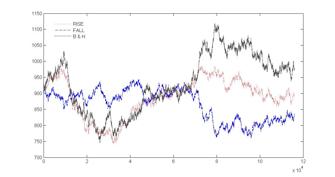
Figure 4: Evolution of capitals of three trading strategies for the period 26.03.10–25.03.11: Buy and Hold – solid line, UN going long – dotted line, UN going short – dashed line. One run of trading is performed with a simulated stock TEST (see Table 1)

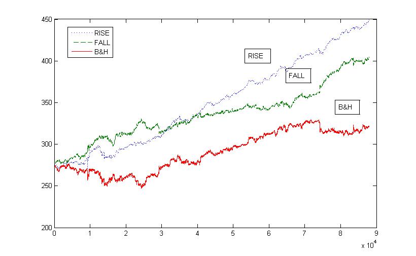
Figure 5: Evolution of capitals of three trading strategies for the period 26.03.10–25.03.11: Buy and Hold – solid line, UN going long – dotted line, UN going short – dashed line. One run of trading is performed with the stock KOCO (see also Table 1)

7 Numerical experiments

Computer technology. In the numerical experiments, we have used historical data in the form of per minute time series of prices of arbitrarily chosen stocks.

Two types of kernel functions were used as the smooth approximations of the combined kernel ${\cal K}(p,p_{n},x,x_{i})=K_{1}(p,x_{n},p_{i},\bar{x}_{i})+K_{2}({\bf x}_{n},{\bf x}_{i})$ from the sum (8): (i) ${\cal K}(p,p_{n})=\cos((\pi(p-p_{n})/2)$, (ii) ${\cal K}(p,p_{n},x,x_{i})=\exp(c(p-p_{n})+c^{\prime}(x-x_{i}))$, where $c,c^{\prime}$ are positive constants.

In any short-term trading algorithm, the time characteristics are crucial. The greatest time cost is associated with the calculation of sums (8) and finding the roots of this equation. The performed experiments show that the computation time for one point of the forecast increases linearly with increasing length of history. To provide one point of time, predicting within 1 - 3 seconds of CPU time, the length of the series was limited up to 5000 points. For series of length greater than 5000 points, “a chain” method of forecasting was used. Two processes working on overlapping intervals of time series are performed at the same time (see Fig 6).

Let $L_{{\rm max}}$ be the chain length, and $L_{{\rm shift}}$ be the value of time shift, where $L_{{\rm shift}}<L_{{\rm max}}$. In any process, the first $L_{{\rm shift}}$ time-points are used only for scaling prices and preliminary learning of the forecasting algorithm. The trading is not performed at first $L_{{\rm shift}}$ time-points of the series.

When a regular process terminates we switch to the time-point $L_{{\rm shift}}+1$ of the next process. The results of parallel computing are accumulated into a single overall forecasting series. We take $L_{{\rm max}}=5000$ and $L_{{\rm shift}}=2000$.

Figure 6: Scheme of parallel computations

The prices of a stock are scaled such that $S_{i}\in[0,1]$ for all $i$. The scaling is performed for time series of each process separately. The first $L_{{\rm shift}}$ time points of any process are used for computing a scaling constant. Prices are scaled as follows:

$$S_{i}=\frac{\hat{S}_{i}}{c\max\limits_{1\leq j\leq L_{{\rm shift}}}\hat{S}_{j}},$$

where $1\leq i\leq L_{{\rm max}}$ and $\hat{S}_{i}$ are real prices of the stock. We set $c=14$.

The forecasting algorithm is performed for the scaled prices $S_{i}$, where $L_{{\rm shift}}+1\leq i\leq L_{{\rm max}}$.

We implement this computer technology for two forecasting algorithms: the universal strategy constructed in Section 3 (UN–model) and Autoregressive Moving Average algorithm (ARMA–model) (see Peng and Aston 2011).

Table 1: Universal trading

	Buy&	UN	UN	ARMA	ARMA
Ticker	Hold	going long	going short	going long	going short
	Profit %	Profit %	Profit %	Profit %	Profit %
TEST	6.85	-1.39	-8.19	9.88	3.08
AT-T	7.71	137.40	129.70	30.73	23.02
CTGR	15.04	1594.34	1579.34	1167.22	1152.53
KOCO	16.55	62.66	46.15	2.90	-13.61
GOOG	10.25	114.85	104.62	12.85	2.62
InBM	24.28	85.38	61.09	29.31	5.02
INTL	4.29	111.70	107.50	25.86	21.66
MSD	10.71	58.32	47.60	18.66	7.95
US1.AMT	22.01	22.74	0.77	28.46	6.49
US1.IP	2.40	19.83	17.47	9.36	7.00
US2.BRCM	25.30	53.62	28.28	20.06	-5.27
US2.FSLR	40.15	143.92	103.61	-9.86	-50.16
SIBN	-6.54	732.87	739.33	357.74	364.20
GAZP	22.75	101.20	78.45	31.75	9.00
LKOH	19.39	261.84	242.45	87.08	67.68
MTSI	-1.61	669.16	670.68	326.12	327.64
ROSN	9.69	188.89	179.12	34.40	24.63
SBER	14.21	108.97	94.90	37.53	23.46

Results of numerical experiments. In the numerical experiments, we have used historical data in form of per minute time series of prices of arbitrarily chosen 17 stocks (11 US stocks, and 6 Russian stocks) and of one simulated stock TEST. Data has been downloaded from FINAM site: www.finam.ru. Number of trading points in each game is N=88000–116000 min. (From March 26 2010 to March 25 2011).

The artificial stock TEST is simulated as $S_{i}=S_{i-1}+\xi_{i}$, $i=1,2,\dots,N$, where $\xi_{i}$ is the Gaussian random variable with mean 0 and a variance equal to the variance of the scaled GAZP stock.

We implement the trading strategy defined in Section 4.

Two series of numerical experiments were performed.

In the first series, we use the trading strategy $\tilde{M}_{i}$ studied in Theorem 5. At each step, starting from initial capital ${\cal K}_{0}^{R}={\cal K}_{0}^{F}={\cal K}_{0}=KS_{0}$, where $S_{0}$ is the price of a stock at the first time point, this strategy performs going long or for going short with $K$ shares of the stock. We take $K=5$ in our experiments. In case of going long, the capital changes at any step $i$ as ${\cal K}_{i}^{R}={\cal K}_{i-1}^{R}+K(S_{i}-S_{i-1})$ if $\tilde{p}_{i}>\tilde{S}_{i-1}$ and ${\cal K}_{i}^{R}={\cal K}_{i-1}^{R}$ otherwise. In case of dealing for a fall ${\cal K}_{i}^{F}={\cal K}_{i-1}^{F}-K(S_{i}-S_{i-1})$ if $\tilde{p}_{i}\leq\tilde{S}_{i-1}$ and ${\cal K}_{i}^{F}={\cal K}_{i-1}^{F}$ otherwise, where $i=1,2,\dots,N$.

Results of numerical experiments are shown in Table 1. In the first column, stocks ticker symbols are shown. The second column contains the profit of Buy-and-Hold trading strategy. By this strategy, we buy a holding of shares using capital ${\cal K}_{0}$ and sell them for ${\cal K}_{N}$ at the end of the trading period.

Table 2: Defensive trading

	Buy&	UN	UN	ARMA	ARMA	UN	ARMA	UN	ARMA
Ticker	hold	Profit	Profit	Profit	Profit
	%	%	-0.01%	%	-0.01%	In	In	D	D
TEST	6.85	3.58	-80.93	3.58	-80.90	0.232	0.163	1.453	1.890
AT-T	7.71	69.01	-79.19	29.86	-79.19	0.218	0.205	1.611	1.576
CTGR	15.04	1030.12	658.13	937.46	540.18	0.238	0.253	1.654	1.479
KOCO	16.55	36.47	-78.62	15.69	-78.55	0.216	0.198	1.604	1.502
GOOG	10.25	46.54	-80.57	3.53	-82.68	0.231	0.211	1.462	1.474
InBM	24.28	54.79	-78.53	34.66	-78.10	0.219	0.187	1.514	1.517
INTL	4.29	43.06	-76.60	5.63	-76.28	0.220	0.179	1.630	1.585
MCD	10.71	34.22	-78.56	19.21	-78.41	0.222	0.190	1.571	1.876
AMT	22.01	16.47	-77.01	24.04	-77.09	0.212	0.183	1.654	1.758
IP	2.40	4.45	-82.78	-14.79	-81.06	0.213	0.181	1.657	1.760
BRCM	25.30	11.40	-80.47	23.98	-76.10	0.216	0.172	1.585	1.876
FLSR	40.15	21.02	-80.04	-27.50	-80.03	0.227	0.196	1.499	1.506
SIBN	-6.54	600.62	249.87	287.48	-58.55	0.169	0.179	2.460	2.292
GAZP	22.75	51.29	-82.04	4.34	-82.16	0.224	0.210	1.539	1.526
LKOH	19.39	149.03	-79.91	46.44	-80.62	0.230	0.244	1.527	1.501
MTSI	-1.61	482.83	79.23	275.13	-69.36	0.188	0.195	2.174	1.959
ROSN	9.69	101.15	-83.14	-0.53	-83.54	0.228	0.240	1.549	1.499
SBER	14.21	51.56	-82.52	-14.47	-82.73	0.225	0.196	1.559	1.674

In the 3th and 4th columns, results of one run of trading based on the universal randomized forecasting strategy (UN) are shown. In the 3th column, a relative return, percentagewise, to the initial capital $\frac{{\cal K}_{N}-{\cal K}_{0}}{{\cal K}_{0}}100\%$ is shown for going long, in the 4th column, the same relative return is shown for going short, In the 5th and 6th columns, the same results are shown for trading using ARMA forecasts.

It was found that ${\cal K}_{i}>0$ for $i=1,2,\dots,N$, i.e., we never incur debt in our experiments (with an exception of TEST stock).

Results presented in Table 2 show that trading based on UN model of forecasting performs at least as well as the trading based on ARMA forecasting model and essentially outperforms it for some stocks.

The second series of experiments is closer to a real short-term trading. The trading strategy has a defence guarantee. Starting with the same initial capital ${\cal K}_{0}=KS_{0}$, where $S_{0}$ is the initial price of a stock and $K=5$, we perform going long using “a defensive” trading strategy. At any step $i$, our working capital is ${\cal L}_{i-1}=\min\{{\cal K}_{0},{\cal K}_{i-1}\}$. Using this capital, we buy $M_{i}={\cal L}_{i-1}/S_{i-1}$ shares of the stock at the beginning of any step $i$, if ${\cal L}_{i-1}>0$, and stop trading otherwise: $M_{i}=0$. We update the cumulative capital at the end of each step: ${\cal K}_{i}={\cal K}_{i-1}+M_{i}(S_{i}-S_{i-1})$. Thereby, we can set aside the extra income.

Results of second series of numerical experiments are shown in Table 2. In the first column, stocks ticker symbols are shown. The second column contains the relative return of Buy-and-Hold trading strategy. In the next pair of columns marked “UN”, relative returns of one run of randomized trading, percentagewise, for the initial capital are presented for the case with no transaction costs and for the case where transaction cost at the rate $0.01\%$ is subtracted. We compute the forecast of a future stock price by the method of calibration and defensive forecasting (UN) presented in Theorem 1.

The next two columns marked by “ARMA” are similar, with the exception that the ARMA forecasting model is used for computing forecasts. The frequencies of market entry steps $i$, where $\tilde{p}_{i}>\tilde{S}_{i-1}$, are given in the next two columns marked “In” (for UN and ARMA). We sell all shares of a stock at step $i$ in case $\tilde{p}_{i}\leq\tilde{S}_{i-1}$. The average time spent in the market is shown in the rest two columns marked “D” (for UN and ARMA).

8 Acknowledgement

This research was partially supported by Russian foundation for fundamental research: Grant 13-01-12447 and 13-01-0052.

9 Conclusion

Asymptotic calibration is an area of intensive research where several algorithms for computing well-calibrated forecasts have been developed. Several applications of well-calibrated forecasting have been proposed (convergence to correlated equilibrium, recovering unknown functional dependencies, predictions with expert advice). We present a new application of the calibration method.

We show that the universal trading strategy can be constructed using the well-calibrated forecasts. We prove that this strategy performs at least as well as any stationary trading strategy presented by a rule from any RKHS with regret $O(n^{\frac{3}{4}})$. Using the universal kernel, we prove that this strategy performs at least as good as any stationary continuous trading strategy.

The obvious drawback of a universal strategy is that it uses the high frequency trading, which prevents it from practical applications in the presence of transaction costs.

To construct the universal trading strategy, we generalize Kakade and Foster’s algorithm and combine it with Vovk’s DF–model for arbitrary RKHS. Using Vovk (2006) theory of defensive forecasting in Banach spaces, these results can be generalized to these spaces.

Unlike in statistical theory, no stochastic assumptions are made about the stock prices.

Numerical experiments show a positive return for all chosen stocks, and for some of them we receive a positive return even when transaction costs are subtracted. Results of this type can be useful for technical analysis in finance.

References

Blackwell (1956)
D. Blackwell. An analog of the minimax theorem for vector payoffs.
Pacific Journal of Mathematics, 6, 1956, 1–8
Chernov et al. (2010)
A. Chernov, Y. Kalnishkan, F. Zhdanov, V. Vovk.
Supermartingales in Prediction with Expert Advice.
Lecture Notes in Computer Science, 5254, 2008, 199–213
Cesa-Bianchi and Lugosi (2006)
N. Cesa-Bianchi, G. Lugosi.
Prediction, Learning and Games. Cambridge University Press, 2006
Cover and Gluss (1986)
T. Cover, D. Gluss. Empirical Bayes stock market portfolios.
Advances in Applied Mathematics, 1986, 7, 170 -181.
Cover and Ordentlich (1996)
T. Cover, E. Ordentlich. Universal portfolio with side information.
IEEE Transaction on Information Theory, 42. 1996, 348–363
Cristianini and Shawe-Taylor (2000)
N. Cristianini, J. Shawe-Taylor. An Introduction to Support Vector
Machines and other kernel-based learning methods.
Cambridge University Press, Cambridge, 2000.
Dawid (1982)
A.P. Dawid. The well-calibrated Bayesian [with discussion].
J. Am. Statist. Assoc. 77, 1982, 605–613
Dawid (1985)
A.P. Dawid.
Calibration-based empirical probability [with discussion].
Ann. Statist., 13, 1985, 1251–1285