FRW type of cosmology with a Chaplygin gas
D. Panigrahi111 Sree Chaitanya College, Habra 743268, India
and also Relativity and Cosmology Research Centre, Jadavpur
University, Kolkata - 700032, India , e-mail:
dibyendupanigrahi@yahoo.co.in
and S. Chatterjee222 IGNOU Convergence
Centre, New Alipore College, Kolkata - 700053, India and
also Relativity and Cosmology Research Centre, Jadavpur
University,
Kolkata - 700032, India, e-mail : chat_sujit1@yahoo.com
Correspondence to
: S. Chatterjee
Abstract
The evolution of a universe modelled as a mixture of generalised Chaplygin gas and ordinary matter field is studied for a Robertson Walker type of spacetime. This model could interpolate periods of a radiation dominated, matter dominated and a cosmological constant dominated universe. Depending on the arbitrary constants appearing in our theory the instant of flip changes. Interestingly we also get a bouncing model when the signature of one of the constants changes. The velocity of sound may become imaginary under certain situations pointing to a perturbative state and consequently the possibility of structure formation. We also discuss the whole situation in the backdrop of wellknown Raychaudhury equation and a comparison is made with the previous results.
KEYWORDS : cosmology; accelerating universe; chaplygin gas
PACS : 04.20, 04.50 +h
1 Introduction
Three discoveries in the last century have radically changed our
understanding of the universe - as opposed to the idea of
Einstein’s static universe Hubble and Slipher(1927) showed that it
is expanding. Secondly CMBR as also primordial nucleosynthesis
analysis in the sixties point to an initial hot dense state of the
universe, which has been expanding for the last 13.5 Gyr. Finally,
if we put faith in Einstein’s theory and FRW type of model then as
standardised candles type Ia supernova suggest [1] that the
universe is undergoing accelerated expansion with baryonic matter
contributing only five percent of the total energy budget. Later
data from CMBR probes [2] also point to the same finding.
This has naturally led a vast chunk of cosmology community to
embark on a quest to attempt to explain the cause of the apparent
acceleration. The vexed question in this field is the possible
identification of the processes likely to be responsible for
triggering the late inflation. Researchers are plainly divided
into two broad groups - either modification of the original
Einstein’s theory or introduction of any exotic type of fluid like
a cosmological constant or a quintessential type of scalar field.
But the popular explanation with the help of a cosmological
constant is beset with serious theoretical problems because
absence of acceleration at redshifts implies that the
required value of the cosmological constant is approximately 120
orders of magnitude smaller than its natural value in terms of
Planck scale [3]. As for the alternative quintessential
field [4] we do not in fact have a theory that would
explain, not to mention predict, the existence of a scalar field
fitting the bill without violating the realistic energy
conditions. Moreover we can not generate this type of a scalar
field from any basic principles of physics. Other alternatives
include k-essence [5], tachyon [6],
phantom [7] and quintom [8]. So there has been a
resurgence of interests among relativists, field theorists,
astrophysicists and people doing astroparticle physics both at
theoretical and experimental levels to address the problems
emanating from the recent extra galactic observations without
involving any mysterious form of scalar field by hand but looking
for alternative approaches based on sound physical principles.
Alternatives include, among others, higher curvature theory,
axionic field and also Brans- Dicke field. Some people attempted
to look into the problem from a purely geometric point of view -
an approach more in line with Einstein’s spirits. For example,
Wanas [9] introduced torsion while
Neupane [10, 11] modifies the spacetime with a warped
factor in 5D spacetime in a brane like cosmology and finally
addition of extra spatial dimensions in physics as an offshoot of
prediction from the string theory [12, 13, 14, 15, 16].
While this torsion inspired inflation has certain desirable
features the problem with Wanas’ model is that the geometry is no
longer Riemannian. Further a good number of
people [17, 18, 19, 20] have done away with the concept of
homogeneity itself and have argued that accelerating model and
consequent introduction of exotic matter field have to be invoked
only in FRW type of cosmology. In Tolman Bondi like inhomogeneous
model the apparent dimming of the signals may be explained as a
consequence
of inhomogeneous distribution of matter.
While the above mentioned alternatives to explain away the
observed acceleration of the current phase have both positive and
negative aspects the one that caught the attention of a large
number of workers is the introduction of a Chaplygin type of gas
as new matter field to simulate a sort of dark energy. The form of
the matter field is later generalised through the addition of an
arbitrary constant as exponent over the mass density and is
generally referred to as generalised chaplygin
gas(GCG) [21, 22]. Though it suffers from the serious
disqualification that it violates the time honoured principle of
energy conditions its theoretical conclusions are found to be in
broad agreement with the observational results coming out of
gravitational lensing or recent CMBR and SNe data in varied cosmic
probes [23, 24]. This is generally achieved through a
careful maneuvering of the value of the newly introduced arbitrary
constant. To further fine tune the match between the theory and
the very recent observational fallouts the GCG is again modified
via the addition of an ordinary matter field, which is termed in
the literature as modified chaplygin gas(MCG) [25, 26].
The viability of such scenarios has been tested by a number of
cosmological probes, including SNe Ia data [23, 24],
lensing statistics [27, 28, 29], age-reshift
tests[30], CMB measurements [31], measurements
of X Ray luminosity of galaxy clusters [32], statefinder
parameters [33]. In our previous work [34] we have
studied Chaplygin gas model in inhomogeneous space time. In the
present work we have revisited the dynamics of the FRW model
taking MCG as matter field and have tried to discuss some as yet
unexplored region and have got some interesting results. We have
organised the paper as follows: In section 2 the mathematical
formulation is given and we have ended up with a hypergeometric
solution and also an effective equation of state as in section 3. So depending on initial conditions
our model mimics both and quiessence models and the
evolution is also shown graphically. We have also made some
detailed discussion on acoustic wave in our model and find that
all possibilities like less/greater than light velocity and even
imaginary values exist in our model. Relevant to mention that
imaginary sound velocity is not that much discouraging in this
context because it gives rise to perturbation and consequent
structure formation [35]. The interesting thing in our
analysis is that we have taken the first order approximation of
the field equation as key equation and subsequently found out the
exact solutions. We are not aware of attempts of similar kind in
the past literature. Moreover it is also found that if an
arbitrary constant appearing in our solution be taken negative the
cosmology bounces back from a minimum. We have also made a
detailed analysis of flip time both analytically and graphically
in this section. In section 4 these conclusions are checked in the
framework of well known Raychaudhury equation. The paper ends with
a discussion in section 5.
2 Field Equations
We consider a spherically symmetric homogeneous spacetime given by
| (1) |
where the scale factor, depends on time only.
A comoving coordinate system is taken such that and where is the 4- velocity. The energy momentum tensor for a dust distribution in the above defined coordinates is given by
| (2) |
where is the matter density and the isotropic pressure.
The independent field equations for the metric (1) and the energy momentum tensor (2) are given by
| (3) |
| (4) |
From the the Bianchi identity we get for the homogeneous model the conservation law
| (5) |
which, in turn, yields
| (6) |
At this stage we assume that we are dealing with a Modified Chaplygin type of gas (MCG) obeying an equation of state
| (7) |
where and are constants. The exponent , from most observational constraints, hovers around unity [36] and the constant ranges from to zero. Similarly the positive definite constant is also not exactly arbitrary. In the equation (7) when the last two terms start to be of the same order of magnitude the pressure vanishes. In this case the fluid has pressureless density corresponding to some cosmological scale given by . Many variants of Chaplygin gas model have come up in the literature and the equation (7) refers to what is generally known as the Modified Chaplygin gas model (MCG) [25, 26] such that gives generalized model (GCG) [31] and if in addition one recovers the original model. Moreover, the first term on the r.h.s. of the equation (7) gives an ordinary fluid obeying a barotropic equation of state (EoS) so that we here are essentially dealing with a two fluid model. Further, the equation (7) points to an EoS that interpolates between standard fluids at high energy densities and Chaplygin gas fluids at low energy densities. In the 4D framework the dynamics of the MCG model has been studied in the reference [25, 26] and a perturbative study looking for some generic features is carried out in [37]. On the other hand Fabris et al [38], in an interesting work, have used a perturbative analysis to confront observational data within this model and taking the particular case of power spectrum observational data have concluded that the recent data restricts the value of such that the GCG is recovered and the MCG is almost ruled out. Moreover, in the case of MCG model recent supernova data seem to favour negative values of the parameter [39]. When one attempts to address issues concerning structure formation the study of cases with negative values of becomes more sensible since this implies imaginary sound velocities, hence plagued with the possibility of instabilities [40, 23, 24]. On the other hand it has been argued that is also plausible [41]. With the help of equations (6) & (7) a little mathematics shows that an expression for density comes out to
| (8) |
where is an integration constant. The above equation (8) yields a first integral as
| (9) |
Plugging in the expression of from equations (3) and (9) we finally get
| (10) |
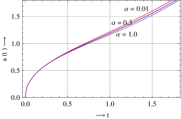
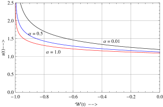
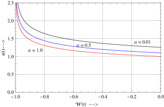
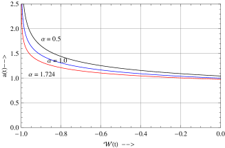
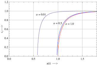
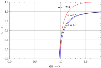
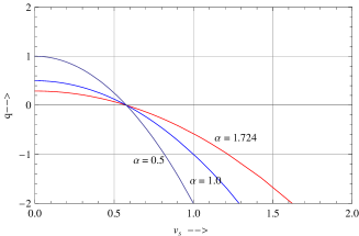
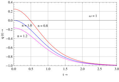
Using equation (10) we have drawn the figure-1, where the evolution of with
is shown. This figure shows that as increases the rate of change of scale factor
decreases. A cursory look at the equation also points to this type
of variation of the curves. In fact the equation (10) suggests
that with ,
becomes flatter.
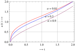
At this stage if we consider (figure-1b) we get from the equation (7) that as increases () the first term on the r.h.s. reduces to zero while the second term decreases for a particular . We get identical results for (figure-1c). Now, being a small fraction at the late stage of evolution of the universe any increase in its value in the exponent finally increases its magnitude so that the pressure becomes more negative, which, in turn drives the expansion more vigorously.
Our analysis is based on different sets of observational data. By using a large sample of milli-arc second radio sources recently updated and extended by Gurvits et al [42] along with the latest SNeI data as given by Reiss et al [43], Alcaniz and Lima [44] showed that the best fit data for these observations are (UDME) and (CGCDM), where , where is the present density of the Chaplygin gas. In another work Lima et al [36] showed at confidence level by the BAO (Baryon acoustic Oscillation) and Gold sample analysis, the range of is while BAO SNLS analysis provides . Both the results predict to be nearly equal to unity. In contrast to this result Fabris et al [38] as pointed out earlier ruled out the existence of for the MCG model in the context of power spectrum observational data. In this context the relations and seem interesting. When the value of is nearly equal to unity there remains a tiny value of , which is not exactly in line with the work of Fabris et al [38]. Lastly Lu et al [41] gives for the MCG best fit data and in the light of 3 yr WMAP and SDSS data.
3 Cosmological dynamics
It is very difficult to get the exact temporal behaviour of the scale factor, from the equation (10) in a closed form because integration yields elliptical solution only. However, the equation (10) does give significant information under extremal conditions as briefly discussed below.
Deceleration Parameter:
At the early stage of the cosmological evolution when the scale factor is relatively small the second term of the last equation (10) dominates which has been already discussed in the literature [25, 26]. So we will be very brief on this point. From the expression of the deceleration parameter, we get
| (11) |
where is the Hubble constant. With the help of the EoS given by (7) we find
| (12) |
which via equation (9) gives
| (13) |
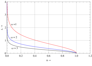
As the universe expands decreases with time such that the second term in the equation(12) increases pointing to the occurrence of a flip when the density attains a critical value given by . This flip density depends on the exponent such that at the larger value of the flip density decreases, i.e., flip occurs at a lower density, i.e., it occurs at a later time. We know from Lima’s [36] that the value of is restricted to such that acceleration is a recent phenomenon. This result is encouraging. As discussed in the last Section Lu et al [41] argued that also conforms to the observational analysis. This finding is particularly relevant to our case in the sense that higher values of signify a lower , i.e., more recent accelerating phase. The above analysis in conformity with the nature of curve in figure-2.
CASE A : At the early stage when the scale factor, is very small the equation (13) reduces to
| (14) |
Evidently the deceleration parameter has contribution from the baryonic matter content only such that, mimcs the ordinary fluid behaviour with magnitudes and for radiation and dust respectively as in a FRW model. When the equation (14) gives, evolving as a model.
CASE B : In earlier works [25, 26] authors utilized the above equations to find an equation of state at the late stage of evolution as, .
Using the equations (7) (9) straightforward calculations yield an effective EoS at the late stage of evolution as
| (15) |
where
| (16) |
which is a function of time only. This is clearly at variance with the earlier works of [25, 26] where the effective EoS shows no time dependence. We also find that at the late stage of evolution as , so we asymptotically get from this Chaplygin type of gas, which corresponds to an empty universe with cosmological constant such that the equation (11) implies that the deceleration parameter, reduces to . Interestingly always remains greater than , thus avoiding the undesirable feature of big rip. In this context we call attention to a recent work of Z. K. Guo and Y. Z. Zhang [45] where a new variant of CG is taken in the form of
| (17) |
where unlike the original CG, is taken as a function of the scale factor . For mathematical simplicity they assumed where and are constants and and . They finally end up with a constant equation of state parameter
| (18) |
We find that corresponds to the original Chaplygin gas model
which interpolates between a universe dominated by a dust and
DeSitter era. Moreover corresponds to a quiessence dominated
and to a phantom dominated model. In our case we, however, get here a time
dependent equation of state parameter which always avoids the undesirable
phantom like behaviour.
To end up a final remark may be in order. In an earlier work the present authors [12, 13] in the framework of homogeneous spacetime studied the scenario with an EoS given by equation(7) but generalised to extra dimension. Using an ansatz where and are 3D and extra dimensional scale factors and is a constant has led us, at the late stage, to an EoS . The expression for the is found to be
| (19) |
where , is a constant. Unlike the usual 4D cases (see for example [46]), here . Obviously this is due to the presence of extra dimensions in the above relation. In 4D case () and a model is the only possibility. In general the magnitude of is parameter dependent and presents varied possibilities. When , i.e. is a constant we again get back the 4D case. When , ; So a phantom like cosmology results with the occurrence of ‘big rip’ etc. But the cosmology becomes physically interesting when such that and we get a quiessence type of model [47, 48].
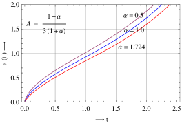
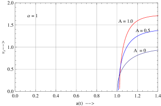
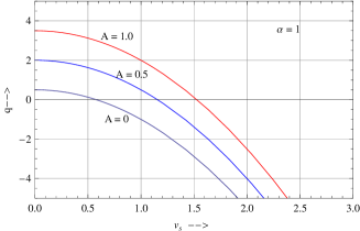
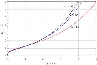
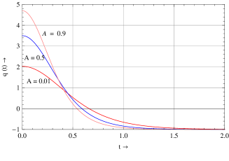
The variation of with the scale factor for different values of are shown in the figure-3. We have considered three cases: the constant value of is chosen for the figure 3a, on the other hand we have chosen the relation and for the figure 3b and 3c respectively. All the graphs clearly show that the scale factor increases as becomes more and more negative.
Since, , the relation shows that can never be less than , a good sign. Otherwise there will be a phantom stage. In quintessence model starts from zero and then reduces to .
Acoustic wave :
In this case the expression of the velocity of sound with the help of equation (15) will be
| (20) |
Using equations (11) and (20) we get the expression of the deceleration parameters,
| (21) |
We have considered three relations for as , and to study the above equations in a more transparent manner. From the observational point of view it is seen that the value of is nearly equal to the unity. As pointed out earlier Fabris et al [38] studied and ruled out the constant . However, our investigations differ and in a sense more general than Fabris et al [38] in that we have allowed a small value of for [36]. When , we get the negative value of which also is in agreement with some observational result [41].
I. :
From equation (20) we get
| (22) |
The equation (22) shows that for , is always less than the velocity of light and can not be imaginary. For any other values of A (the limit of is ) the velocity of sound may not be less than . Now with the help of the equation (20) we calculate the condition for which is
| (23) |
On the other hand there may be a possibility for , but our discussion is restricted only to the late stage of evolution where the scale factor is large enough. In this context we get at the late stage of evolution. The above phenomenon is shown graphically in the figure-4a.
II: : From equation (20) we get
| (24) |
It is evident from the equation (24) as well as from the figure-4b that the velocity of sound always less than the velocity of light for any value of ( since ). For , and we get back the situation depicted in the figure-4a, however, for any other values of (), . Some observations predict that the value of is nearly equal to [36]. So for the maximum permissible value of , should be always less than the velocity of the light . But in the previous case ( for equation (22)), there may be a possibility that the is greater than [49] for the high value of i.e., at the very late stage of evolution. We also get the same conclusion from the equation (23).
III: :
From equation (20) we get
| (25) |
For late universe when is very large, the above equation
reduces to . When
i.e., we get back to the model, in this
case and for (in this case ), i.e., for pure Chaplygin gas model, which
imply that for , . Again for
, we have seen that , however, violates
the causality condition. The figure-4c gives similar conclusion.
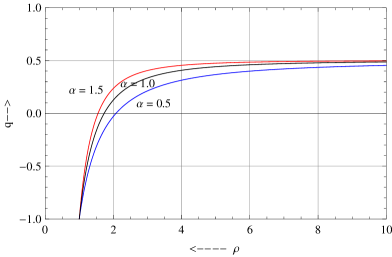
Now we discuss the whole analysis of in the context of deceleration parameter using equation (21). To get accelerating universe should be negative. So the condition for accelerating universe involving is .
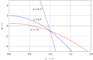
From the figure-5a it is seen that flip occurs for when . But for other values of , at the time of flip, . In the figure-5b 5c at the time of flip, is always less than for different values of or
Now our analysis will be restricted within the accelerating phase, i.e., after flip. For , to get acceleration . If we consider , i.e., when only the original chaplygin type fluid is present, . So the velocity of sound may or may not be greater than the velocity of light. For , the above expression for the velocity of sound further implies that in order that . In this case we restrict the limit of as . Again when , to get acceleration, . For , exactly similar to the situation discussed earlier. When , . For or , but for , negative value.
CASE C : Distinctly new models unfold itself when we take the arbitrary integration constant as . Here the energy density increases with the scale factor mimicing a phantom dark energy model and finally ending up as a cosmological constant. We get from (15) that for the matter field to be well behaved the condition
| (26) |
need to be satisfied. So a minimal value of the scale factor given by
| (27) |
This naturally points to a bouncing cosmology at early times. In
the past Setare [50] analysed these possibilities in a
series of work. To sum up we see that the Chaplygin model
interpolates between a dust at small and a cosmological
constant at large but this well formulated quartessence idea
breaks when a negative value of the arbitrary constant is taken.
Following Barrow [46] if we reformulate the dynamics with a
scalar field and a potential to simulate the
Chaplygin cosmology, we find that a negative value of implies
that we transform . In this case the expressions for
the energy density and pressure corresponding to the scalar field
show
that it represents a phantom field.
CASE D :
As we are considering a late evolution of our model the last term in the equation(10) is almost negligible compared to the second term and so the findings coming from a first order approximation of the equation(10) may be of relevance. Here we find an exact solution of the first order approximation of the equation(10). Authors of this work are not aware of attempts of similar kind in any earlier work. So this is clearly a new result. Now from equation (10) we get, as first order approximation the equation at the late stage of evolution
| (28) |
For economy of space we skip the intermediate steps and write the final solution as,
| (29) |
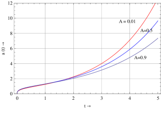
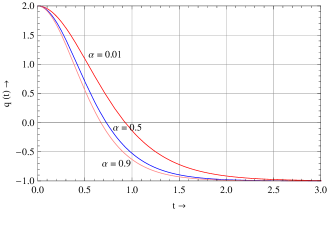
From figure-6 we have seen that the role of the parameters (A and ) are just opposite to what we observe in figure-1. A plausible explanation may be the fact that unlike the first case only first order terms are present here. So the higher order terms in the first case drastically change the scenario and makes their presence felt in changing the nature of the curves. At this stage correspondence to our earlier works [12, 13] may be of relevance. We have shown that one may get similar form of solution in a higher dimensional spacetime if a particular ansatz on the expression of deceleration parameter is taken apriori . But the essential difference between the two lies in the fact that while in the earlier work the hyperbolic solution results from a particular form of the deceleration parameter here we have to invoke a Chaplygin type of gas to get similar comological evolution.
Deceleration Parameter :
The equation (29) can be reduced in the following form
| (30) |
where, , and
such that we get from equation (30)
| (31) |
and
| (32) |
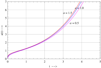
showing that the exponent critically determines the evolution of . A little inspection shows that (i) gives always acceleration, (ii) gives the desirable feature of flip, although it is not obvious from our analysis at what value of redshift this flip occurs. Figure-7 gives the similar conclusion that late flip occurs at lower value of . From equation (31) it further follows that for physically realistic values of and as positive definite and a flip is a distinct possibility, again it follows from equation (31) and also from figure-8 that the early flip occurs at higher values of as well as . Again and depend on and . It can be said that for constant values of and , late flip occurs at higher values of , which have some observational implications that the value of should nearly equal to unity or greater than unity. If we observe the expressions of and , we can not say clearly what values of and give the early flip. But we can say about the time of flip if we consider some special value of .
Now we consider some special cases.
I. :
We get from equations (31) (32) for we get the expression for deceleration parameter
| (33) |
And the flip time can be calculated from the above equation as
| (34) |
If , , we get the evolution dominated by
with no contribution from Chaplygin gas. This also follows from
the equation (34) because here . Thus
there is no flip as in the de-Sitter model.
II. :
Again using equation (31) for we get the expression of the deceleration parameter
| (35) |
From the equation (32) the flip time becomes
| (36) |
III. :
From equation (31) we get
| (37) |
And from equation (32), the flip time becomes
| (38) |
In figure-9, we see that flip depends on . From the graph it is seen that the flip time increase with lower value of . , in agreement with our graph.
4 Raychaudhuri Equation
It may not be out of place to address and compare the situation discussed in the last section with the help of the well known Ray Chaudhuri equation [51], which in general holds for any cosmological solution based on Einstein’s gravitational field equations. With matter field expressed in terms of mass density and pressure Ray Chaudhury equation reduces to a compact form as
| (39) |
in a co moving reference frame. Here is the isotropic pressure and is the energy density from varied sources. Moreover other quantities are defined with the help of a unit vector as under
| (40a) | ||||
| (40b) | ||||
| (40c) | ||||
| (40d) | ||||
We can calculate an expression for effective deceleration parameter as
| (41) |
which allows us to write,
| (42) |
In our case as we are dealing with an isotropic rotation free spacetime both the shear and vorticity scalars vanish.
With the help of the equations (7), (9) & (42) we finally get,
| (43) |
In original Chaplygin gas where we get from the equation (44), . This is exactly similar to what we have found in our earlier work [34] (vide equation 3.11), when dealing with an inhomogeneous LTB model. Now we consider some special cases.
I. :
From Equation (44) we get
| (44) |
In this case flip occurs when , at that time the scale factor will be
| (45) |
Now, at such that acceleration takes place in this case.
II. :
Again using the equation (44) we get
| (46) |
Here, at the flip time and at that time the scale factor will
| (47) |
The acceleration takes place when i.e.
III. :
From equation (44) we get,
| (48) |
Here, at the flip time and at that time the scale factor will
| (49) |
The acceleration takes place when i.e.
In all the cases discussed above (i.e. for different expressions
of ), we find out the conditions such that . The
equations (46), (48) and (49) are consistent in the sense that
when tends to zero
both the expressions for become identical. As discussed in
the end of the last section the observational constraints point to a tiny value of the constant
. At this small value of the expression
in equation (46) is greater than that in
equation (48). Since is a monotonically increasing function of time we get similar
results from the
Ray Chaudhury equation also in respect of the flip time which is
discussed in the previous section
for small values of . If we consider the equation (49)
for as Lu’s [41] choice, in this
case (which is close to Lu’s data) such
that .
5 Concluding Remarks
Here we have considered the homogeneous FRW model with Modified Chaplygin type gas. Our analysis is based on the results of different sets of observational data. There is a continued debate on the exact range of the values of the exponent, which generalizes the original chaplygin gas. While most observations point to the value of as nearly equal to unity but existing literature abounds with examples of, , which incidentally may give . This results in a perturbation of the spacetime and a perturbative analysis of the whole system shows that it favours structure formation. While no basic agreement is reached most workers narrow down the range as is . Lu et al [41] gives for the MCG best fit data and . In these context we have considered , and which are in basic agreement with the observational analysis. Our findings are summarised as follows:
1. As is well known it is very difficult to get exact form of solution of the field equations so we have studied graphically the variation of scale factor with for different values of . The figure shows that as increases the rate of change of scale factor decreases.
2. We have studied the key equation (10) with the help of deceleration parameter. From the definition of the deceleration parameter we have calculated the flip density . At the larger values of the decreases, i.e., flip occurs at lower density or at a later time. Since the acceleration is a recent phenomena, this result is in agreement with the observational analysis that the value of is nearly equal to the unity ( is ). From the figure-2 it is seen that is lower for the higher values of .
3. Since our universe is accelerating our discussion emphasizes only the late stage of evolution. In case B we get a time dependent effective equation of state . It gives at the late stage of evolution as , . So we asymptotically get from this Chaplygin type of gas, which corresponds to an empty universe with cosmological constant such that the equation (11) implies that the deceleration parameter, tries to attain to . Interestingly always remains greater than , thus avoiding the undesirable feature of big rip. Z. K. Guo and Y. Z. Zhang [45] considered the new variant of CG as where and are constants and and . They finally end up with a constant equation of state parameter. In this case they got the EoS parameter , which is time independent. However, in our case we can avoid big rip without introducing any extra parameter.
4. We have studied the velocity of sound in the Modified Chaplygin Gas model. Here we have discussed the possibility of the speed of is greater than the speed of light. For and , is always less than , but for , exceeds at the late stage of evolution. For and , we get is always less than .
5. Taking first approximation of the r.h.s. of equation (10) we get the equation (28). For , and we get the solution of equation (28) in the exact form of . We have seen that flip depends upon . From the figure-7 it is seen that the flip time increases with lower value of . Moreover the flip time characterized by equation (36) is found greater than that in equation (34) and similarly flip time for the equation (38) is greater than the equation (36). This finding may have some observational implications. So as goes to unity, the higher value, should vanish. This, however, is in agreement with the Fabris contention that recent observations point to a vanishing . Another explanation is that if the value of is greater than unity we get the negative value of as suggested by Lu [41].
6. The whole exercise is discussed in the context of Raychaudhuri
equation. As expected the results are in broad agreement with the
previous findings.
The main drawback of the present analysis is that we have not been
able so far to constrain the model parameters with the help of
observational data as is customary in relevant works in this
field. It would also be a nice idea to use redshifts in place of
cosmic time in most of the equations particularly in drawing the
graphs. That would have been more consistent with the current
nomenclature. Both the issues will be addressed in our future
work.
Acknowledgments
DP acknowledges financial support of ERO, UGC for a Minor Research project. The financial support of UGC, New Delhi in the form of a MRP award as also a Twas Associateship award, Trieste is acknowledged by SC.
References
- [1] Reiss et al, 1998 Astrophys. J. 116, 1009, arXiv: 9805201[astro-ph].
- [2] D. N. Spergel et al, 2003 Astrophys. J. Suppl. 148, 175.
- [3] E. Copeland E, M. Sami and S. Tsujikawa, 2006 Int. J. Mod. Phys. D15, 1753.
- [4] M. Sami and T. Padmanabhan, 2003 Phys. Rev. D67, 083509, arXiv: 0212317[hep-th].
- [5] R. J. Scherrer, 2004 Phys. Rev. Lett. 93, 011301.
- [6] G. W. Gibbons, 2002 Phys. Lett. B 537, 1.
- [7] E. Elizalde, S. Nojiri and S. Odintsov, 2004 Phy. Rev. D 70, 043539.
- [8] Z. K. Guo, Y. S. Piao, X. Zhang and Y. Z. Zhang, 2006 Phy. Rev. D74, 127304, arXiv: 0410654[astro-ph].
- [9] M. I. Wanas, ‘Dark Energy: Is It of Torsion Origin?’, 2009 Proceedings of the first MEARIM, edited by A. A. Hady and M. I. Wannas, P-41, arXiv:1006.2154v1 [gr-qc].
- [10] I. P. Neupane, 2009 Class. Quant. Grav. 26, 195008, arXiv: 0905.2774 [hep-th].
- [11] I. P. Neupane, 2010 Int. J. Mod. Physics D19, 2281, arXiv:1004.0254v2 [gr-qc].
- [12] D. Panigrahi and S. Chatterjee, 2011 Grav. Cosm. 17, 18, arXiv: 1006.0476v1 [gr-qc].
- [13] D. Panigrahi, Y. Z. Zhang and S. Chatterjee, 2006 Int. J. Mod. Phys. A21, 6491, arXiv: 0604079 [gr-qc].
- [14] Varun Sahni amd Yuri Shtanov, 2008 ‘Cosmic Acceleration and Extra Dimensions’ arXiv:0811.3839v1 [astro-ph].
- [15] S. Kachru, R. Kallosh, A. Linde and S. P. Trivedi, 2003 Phys. Rev. D68, 046005, arXiv: 0301240 [hep-th].
- [16] M. S. Carroll and L. Mersini, 2001 Phys. Rev. D 64, 124008.
- [17] Andrzej Krasi´nski, Charles Hellaby, Krzysztof Bolejko and Marie-Nöelle Célérier, 2010 Gen. Rel. Grav. 42, 2453, arXiv: 0903.4070v2
- [18] H. Alnes, M Amarzguioui and Ø Grøn, 2007 JCAP 01, 007, arXiv: 0506449 [astro-ph].
- [19] S. Chatterjee, 2011 JCAP 03, 014.
- [20] C. M. Hirata and U. Seljak, 2005 Phys. Rev. D72, 083501 ; arXiv: 0503582[astro-ph].
- [21] M. C. Bento, O. Bertolami and A. A. Sen, 2002 Phys. Rev. D66, 043507.
- [22] V. Gorini, A. Kamenschik and U. Moschella, 2003, Phys. Rev. D67, 063509, arXiv: 0209395 [astro-ph].
- [23] J. C. Fabris, S. V. B. Goncalves and P. E. de Souza, 2002, arXiv: 0207430 [astro-ph]
- [24] R. Colistete Jr., J. C. Fabris, S. V. B. Goncalves and P. E. de Souza, 2004 Int. J. Mod. Phys. D13, 669, arXiv: 0303338 [astro-ph].
- [25] H. B. Benaoum, 2002, arXiv: 0205140 [hep-th]
- [26] U. Debnath, A. Banerjee and S. Chakraborty, 2004 Class. Quant. Grav.21, 5609, arXiv: 0411015 [gr-qc].
- [27] A. Dev, J. S. Alcaniz and D. Jain, 2003 Phys. Rev. D67, 023515, arXiv: 0209379 [astro-ph].
- [28] P. T. Silva and O. Bertolami, 2003 Astrophys. J. 599, 829, arXiv: 0303353[astro-ph].
- [29] A. Dev, D. Jain and J. S. Alcaniz, 2004 Astron. Astrophys 417, 847, arXiv: 0311056 [astro-ph].
- [30] J. S. Alcaniz, D. Jain and A. Dev, 2003 Phys. Rev. D67, 043514, arXiv: 0210476 [astro-ph].
- [31] M. C. Bento, O. Bertolami and A. A. Sen, 2003 Phys. Rev.D67, 063003, arXiv: 0210468 [astro-ph].
- [32] J. V. Cunha, J. S. Alcaniz and J. A. S. Lima, 2004 Phy. Rev. D69, 083501, arXiv: 0306319[astro-ph].
- [33] V. Sahni, T. D. Saini and A. A. Starobinsky and U. Alam, 2003 JETP Lett. 77, 201; arXiv: 0210498 [astro-ph].
- [34] D. Panigrahi and S. Chatterjee, 2011 JCAP 10, 002, arXiv: 1108.2433 [gr-qc].
- [35] J. C. Fabris and J. Martin, 1997 Phys. Rev. D55, 5205.
- [36] J. A. S. Lima, J. V. Cunha and J. S. Alcaniz, 2008 Astropart. Phys 30,196, arXiv: 0608469 v1 [astro-ph].
- [37] S. Costa, M. Ujevic and A. F. dos Santos, 2008 Gen. Rel. Grav. 40, 1683.
- [38] J. C. Fabris, H. E. S. Velten, C. Ogouyandjou and J. Tossa, 2011 Phys. Lett B694, 289, arXiv: 1007.1011v1 [astro- ph.CO].
- [39] Xue-Mei Deng, 2011 Braz. J. of Physics 41, 333, arXiv: 1110.1913v1 [gr-qc].
- [40] C. E. M. Batista, J. C. Fabris and M. Morita, 2010 Gen. Rel. and Grav. 42,839, arXiv: 0904.3948 v1[gr-qc].
- [41] Lu et al, 2008 Physics Lett B 662, 87, arxiv: 1004.3364 [astro-ph].
- [42] L. I. Gurvits, K. I. Kellermann and S. Frey, 1999 Astron. and Astrop. 342, 378, arXiv: 9812018 [astro-ph].
- [43] A. Riess et al, 2004 Astrophys. J. 607, 665, arXiv: 0402512 [astro-ph].
- [44] J. S. Alcaniz and J. A. S. Lima, 2005 Astrophys. J. 618 16, arXiv: 0308465v2 [astro-ph].
- [45] Z. K. Guo and Y. Z. Zhang, 2007 Phys. Lett. B 645, 326, arXiv: 0506091 [astro-ph].
- [46] J. D. Barrow, 1988 Nucl. Phys. B 310, 743.
- [47] S. Hannestad and E. Mörtsell, 2002 Phys. Rev. D66, 063508.
- [48] Z. K. Guo, N. Ohta and Y. Z. Zhang, 2005 Phys. Rev. D72, 023504, arXiv: 0505253 [astro-ph].
- [49] V. Gorini, A. Yu Kamenshchik, U. Moschella, O. F. Piattella and A. A. Starobinsky, 2009 Phys. Rev. D80, 104038, arXiv: 0909.0866v3 [gr-qc].
- [50] M. R. Setare, 2007 Eur. Phys. J. C52, 689, arXiv: 0711.0524 [gr-qc].
- [51] A. K. Raychaudhuri, 1955 Phys. Rev. 98, 1123.