EFFICIENT TOPOLOGY-CONTROLLED SAMPLING OF IMPLICIT SHAPES

Abstract

Sampling from distributions of implicitly defined shapes enables analysis of various energy functionals used for image segmentation. Recent work [1] describes a computationally efficient Metropolis-Hastings method for accomplishing this task. Here, we extend that framework so that samples are accepted at every iteration of the sampler, achieving an order of magnitude speed up in convergence. Additionally, we show how to incorporate topological constraints.

1 Introduction

For many Bayesian inference tasks, evaluating marginal event probabilities may be more robust than computing point estimates (e.g. the MAP estimate). Image segmentation, particularly when the signal-to-noise ratio (SNR) is low, is one such task. However, because the space of shapes is infinitely large, direct inference or sampling is often difficult, if not infeasible. In these cases, Markov chain Monte Carlo (MCMC) sampling approaches can be used to compute empirical estimates of marginal probabilities. Recently, Chang et al. [1] derived an efficient MCMC method for sampling from distributions of implicit shapes (i.e. level sets). We improve upon that algorithm in two ways. First, we improve the convergence rate by defining a Gibbs-like iteration in which every sample is accepted and, second, we demonstrate how to efficiently incorporate both local and global topological constraints on sample shapes.

Many approaches formulate image segmentation as an energy optimization. One can derive a related Bayesian inference procedure by viewing the energy functional $E(\ell;x)$ as the log of a probability function

$$p_{L|X}(\ell|x)\propto\exp\left[\pm E(\ell;x)\right],$$ (1)

where $\ell$ is the labeling associated with some segmentation, $x$ is the observed image, and the $\pm$ in the exponent depends on whether one is maximizing or minimizing. In PDE-based level-set methods, $\ell=\text{sign}(\varphi)$, where $\varphi$ is the level-set function. In graph-based segmentation algorithms, such as ST-Mincut [2] [3] or Normalized Cuts [4], $\ell$ is the label assignment. Often, the energy functional decomposes into a data fidelity term and a regularization of the segmentation (Normalized Cuts being an exception). Bayesian formulations treat the former as the data likelihood and the latter as a prior on segmentations:

$$p_{L|X}(\ell|x)\propto p_{X|L}\left(x|\ell\right)p_{L}\left(\ell\right).$$ (2)

While both the data likelihood and prior terms are user-defined, the form of the prior varies considerably depending on the optimization method; a curve-length penalty is typically used in level-set methods while a neighborhood affinity is typically used in graph-based methods. We refer to these two forms as the PDE-based energy and the graph-based energy, respectively.

Another form of prior information incorporates the topology of the segmented object. Han et al. [5] first showed this using topology-preserving level-set methods, where the topology of the segmented object was not allowed to change. This methodology was later extended in [6] to topology-controlled level-set methods, where the topology was allowed to change but only within an allowable set of topologies. To our knowledge, topology-constrained sampling methods have not previously been considered.

Current methods for sampling implicit shapes include [7], [8], and [1] which all use Metropolis-Hastings MCMC sampling procedures. As shown in [1], the methods of [7] and [8] converge very slowly and cannot accommodate any topological changes. [1], however, presented an algorithm called BFPS that acts directly on the level-set function. BFPS generates proposals by sampling a sparse set of delta functions and smoothing them with an FIR filter. Delta locations and heights were biased by the gradient of the energy to increase the Hastings ratio. Empirical results demonstrated that BFPS was orders of magnitude faster than [7] and [8], and representations, unlike the previous two methods, could change topology. Here, we show how to efficiently sample from a distribution over segmentations in both the PDE-based and graph-based energies. In contrast to previous MCMC samplers, proposals at each iteration are accepted with certainty, achieving an order of magnitude speed up in convergence. Additionally, we incorporate topological control so as to exploit prior knowledge of the shape topology.

2 Metropolis-Hastings MCMC Sampling

We begin with a brief discussion of two MCMC sampling algorithms (c.f. [9] for details). For notational convenience, we drop the dependence on $x$ in distributions. We denote $p_{L|X}(\ell)$ as the target distribution, i.e. the distribution from which we would like to sample. MCMC methods are applicable when one can compute a value proportional to the target distribution, but not sample from it directly. Distributions defined over the infinite-dimensional space of shapes fall into this category. MCMC methods address this problem by constructing a first-order Markov chain such that the stationary distribution of that chain is exactly the target distribution. For this condition to hold, it is sufficient to show that the chain is ergodic and satisfies detailed balance. The Metropolis-Hastings sampler (MH-MCMC) [9] is one such approach. At time $t$ in the chain, the algorithm samples from some user-defined proposal distribution, $\hat{\varphi}^{\left(t\right)}\sim q(\hat{\varphi}^{\left(t\right)}|\varphi^{\left(t-1\right)},x)$, and assigns the transition probability:

$$\varphi^{\left(t\right)}=\begin{cases}\hat{\varphi}^{\left(t\right)}&\text{w/ prob}\quad\min(\alpha^{(t)},1)\\ \varphi^{\left(t-1\right)}&\text{w/ prob}\quad 1-\min(\alpha^{(t)},1)\end{cases},$$ (3)

$$\alpha^{(t)}=\frac{p_{L|X}(\hat{\ell}^{\left(t\right)})}{p_{L|X}(\ell^{\left(t-1\right)})}\frac{q(\varphi^{\left(t-1\right)}|\hat{\varphi}^{\left(t\right)},x)}{q(\hat{\varphi}^{\left(t\right)}|\varphi^{\left(t-1\right)},x)},$$ (4)

where $\alpha^{(t)}$ is the Hasting’s ratio, and the segmentation labels are $\hat{\ell}^{\left(t\right)}=\text{sign}(\hat{\varphi}^{\left(t\right)})$ and $\ell^{\left(t-1\right)}=\text{sign}(\varphi^{\left(t-1\right)})$. As this transition probability satisfies detailed balance, the correct stationary distribution is ensured as long as the chain is ergodic. A single sample from the target distribution is then generated by repeating this proposal/transition step until the chain converges.

2.1 Gibbs Sampling

Gibbs sampling is a special case of MH-MCMC, where the acceptance ratio, $\alpha^{(t)}$, evaluates to one at every iteration. Gibbs proposals typically select a random dimension and sample from the target distribution conditioned on all other dimensions. Empirical evidence (as shown in Figure 1) indicates that when learning appearance models (e.g. in [10]), Gibbs sampling exhibits slow convergence times.

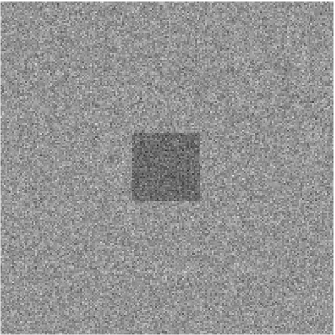
Original

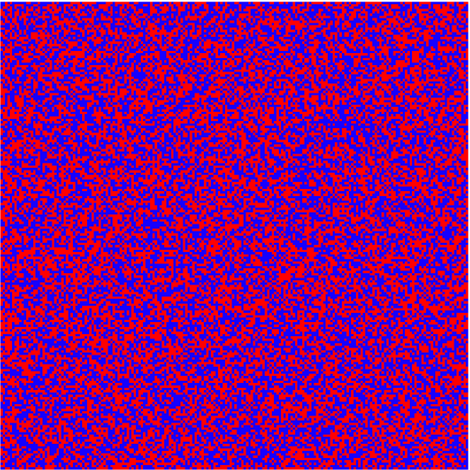
Initialization

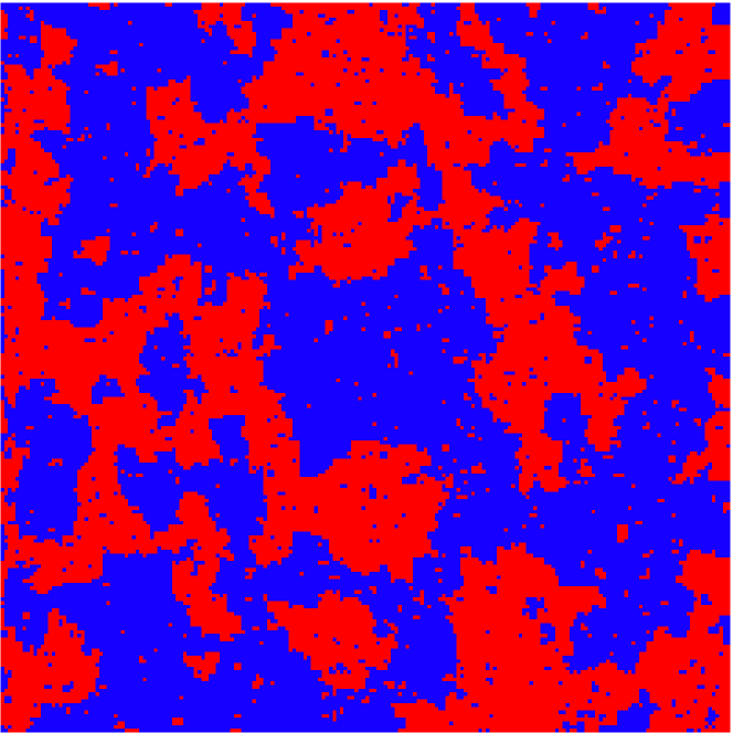
Gibbs

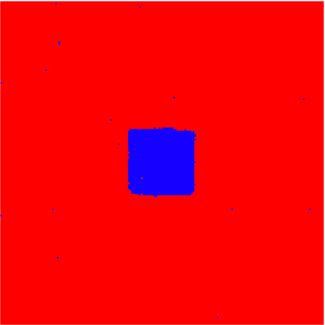
GIMH-SS

Figure 1: An example of the Gibbs sampling getting stuck in a local extrema as compared to the presented GIMH-SS.

Block Gibbs sampling, where a group of dimensions are sampled conditioned on all other dimensions, allows for larger moves. The proposed algorithm is related to this type of Gibbs sampling.

3 Gibbs-Inspired Metropolis-Hastings

BFPS [1] achieves a high acceptance ratio at each iteration by biasing the proposal by the gradient of the energy functional. Here, we design a similar proposal such that samples are accepted with certainty. Given some previous level-set function, $\varphi^{\left(t-1\right)}$, we generate a proposal, $\hat{\varphi}^{\left(t\right)}$ with the following steps: (1) sample a mask, $m$, that selects a subset of pixels and (2) add a constant value, $f$, to all pixels within this mask. We can express this as

$$\hat{\varphi}^{\left(t\right)}(m,f)=\varphi^{\left(t-1\right)}+f\cdot m,$$ (5)

where the mask, $m$, is a set of indicator variables with the same size as $\varphi$. The support of the mask can be of any shape and size, though in practice we use circles of random center and radius. Deferring the choice of $f$, we write the proposal likelihood as

$$q(\hat{\varphi}^{\left(t\right)}|\varphi^{\left(t-1\right)},x)=p_{M}(m)\,p_{F|XM\Phi}(f|m,\varphi^{\left(t-1\right)}).$$ (6)

Figure 2 shows a notional mask overlaid on a level-set function, $\varphi$, with the height of $\varphi$ plotted on the real line for pixels in the support of the mask.

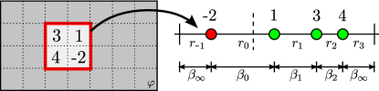
Figure 2: Mapping the masked level-set function (left) onto the real line (right). Possible ranges, $r$, and widths, $\beta$, are shown on the right.

The dotted line marks the zero-height which splits pixels into foreground and background. As all pixels in the support of the mask are summed with the same constant, $f$, choosing an $f$ is equivalent to shifting the zero-height by $-f$. The resulting proposed zero-height can fall into one of $\left(\left|m\right|+1\right)$ different ranges, where $\left|m\right|$ counts the pixels in the support of the mask. The random range, $R$, of the perturbation can take on integers in $[-n^{-},n^{+}]$, where $n^{\pm}$ count the pixels in the support of the mask that have height $\varphi\gtrless 0$.

Sampling a perturbation, $f$, can then be decomposed into sampling a range followed by a value within that range. Most energy functionals only depend on the sign of pixels, which conveniently is determined solely by the range. If we choose $p_{F|R}(f|r)=\frac{1}{\beta_{r}}$ (i.e. a uniform distribution), we can write the perturbation likelihood as

$$p_{FR|XM\Phi}(f|m,\varphi^{\left(t-1\right)})=\frac{1}{\beta_{r}}p_{R|XM\Phi}(r|m,\varphi^{\left(t-1\right)}),$$ (7)

where $\beta_{r}$ is the width or range $r$ (note that $r$ is deterministic conditioned on $f$). Because the value of $f$ within a range $r$ does not affect the sign of the resulting level-set function, the proposed labeling can be expressed as

$$\hat{\ell}^{\left(t\right)}(m,r)=\text{sign}(\hat{\varphi}^{\left(t\right)}(m,f\sim p_{F|R}(f|r)).$$ (8)

By choosing the following Gibbs-like proposal for the ranges,

$$p_{R|XM\Phi}(r|m,\varphi^{\left(t-1\right)})\propto\beta_{r}\,p_{L|X}(\hat{\ell}^{\left(t\right)}(r,m)),$$ (9)

one can verify via Equations 4, 6, and 7 that the Hastings ratio evaluates to one at every iteration.

One subtlety exists in the selection of endpoints for the first and last range. Since these two ranges extend to $\pm\infty$, their corresponding $\beta$ is also $\infty$. We therefore restrict both of these ranges to be of some finite length $\beta_{\infty}$. While any finite value will suffice, in practice, we choose $\beta_{\infty}$ to be $1$. With the endpoint selection for $\beta_{\infty}$, another complication arises. Consider the illustrative distributions for the zero-height line shown in Figure 3.

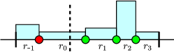
(a)

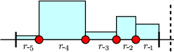
(b)

Figure 3: Example distributions for where the zero-height line can fall. (a) shows an example of a valid proposal, and (b) shows an example of an invalid proposal.

In these examples, some constant $\beta_{\infty}$ is chosen, and the current zero-height line is marked with the dotted line. We can consider these two distributions as two different mask selections. Figure 3a shows what we call a valid mask, in which the current zero-height line falls within the non-zero probability space. Figure 3b, however, shows what we call an invalid mask, in which the current zero-height line falls outside the non-zero probability space. Here, one could propose a forward perturbation such that the resulting proposed zero-height line falls in the non-zero probability space. However, the backward transition to bring the proposed zero-height line back to the current zero-height line would be zero because it lies in the zero-probability space. We note that if $\beta_{\infty}$ is chosen to be some constant $C$, and all pixels are initialized to have height $\left|\varphi_{i}\right|<C$, then every possible (initial) mask will be valid. As the chain progresses, some masks will become invalid, in which case we only sample valid masks. Because any mask that contains both positive and negative pixels is valid, there are always valid masks to sample from.

3.1 Algorithm Description

The resulting algorithm, called the Gibbs-Inspired Metropolis Hastings Shape Sampler (GIMH-SS), is described by the following steps: (1) Sample a circular mask, $m$, with a random center and radius; (2) Sample a range, $r$, according to Equation 9; (3) Sample a perturbation, $f$, uniformly in this range; (4) Compute $\hat{\varphi}^{\left(t\right)}(m,f)$ using Equation 5; (5) Repeat from Step 1 until convergence.

When calculating the likelihood of each range in Step 2, only a value proportional to the true likelihood is needed. Normalization can be performed after the fact because all ranges are enumerated. Equivalently, the energy, which is related to the likelihood via a logarithm, only needs to be calculated up to a constant offset. We therefore compute the change in the energy by including or excluding the pixels in each range. This can be efficiently computed for all ranges using two passes. On each pass, we begin at the range $r_{0}$, setting this energy to zero and choosing to either go in the positive (first pass) or negative (second pass) direction. We then consider $r_{\pm 1}$ and compute the change in energy when the the one pixel changes sign. In graph-based energies, if an $n$-affinity graph is used, only $n$ computations are required at each range evaluation, one for each edge. This procedure is iterated until all ranges are computed (i.e. up through $r_{\pm n^{\pm}}$).

Unlike graph-based energy functionals, the curve length penalty used in PDE-based energy functionals can be a non-local and fairly expensive computation. In optimization-based segmentation algorithms, the evolution of the level-set is based on the gradient of the curve length (i.e. the curvature) which can efficiently be calculated locally. If a subpixel-accurate curve length calculation is required, then the energy functional will indeed depend on the value of the perturbation, $f$, within a particular range, $r$. As an approximation, we compute a pixel-accurate curve length by first setting all pixels on the boundary to have height $\pm 0.5$, initializing a signed-distance function, and then calculating the curve length via

$$\oint_{\mathcal{C}}dl=\int_{\Omega}\delta(\varphi_{i})\left|\nabla\varphi_{i}\right|di\approx\sum_{i}\hat{\delta}(\varphi_{i})\left|\nabla\varphi_{i}\right|,$$ (10)

and the following discrete approximation to the $\delta(\cdot)$ function

$$\hat{\delta}(\varphi_{i})=\begin{cases}1&\left|\varphi_{i}\right|\leq 1\\ 0&\text{else}\end{cases}$$ (11)

If a first-order accurate signed-distance function is obtained using a fast marching method, the height at a particular pixel depends only on pixels in a 3x3 neighborhood. This dependence relationship is illustrated in Figure 4a, where changing the sign of the center black pixel will affect the height of the signed distance function at all the gray pixels. From equation 10, the local curve length calculation depends on the magnitude of the gradient of the level-set function. If a centered finite-difference is used for the $x$ and $y$ directions, then the local curve length computation depends on neighbors above, below, left, and right. Thus, if the heights are changed for the gray pixels in Figure 4a, the curve length computation changes for all the gray pixels in Figure 4b. The change in the curve length for changing the sign of the center pixel is consequently a function of the sign of the 21 pixels in Figure 4b. We precompute all possible $2^{21}$ ($~{}2$ million) combinations so that the curve length penalty can be efficiently computed by a simple table lookup.

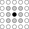
(a)

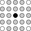
(b)

Figure 4: (a) Signed distance function dependence and (b) curve length penalty dependence.

3.2 Convergence Speeds

To illustrate the performance of GIMH-SS, we run the sampling algorithm on the image shown in Figure 5. We note that this is the same image used in the comparison of [1]. We run each of the four algorithms for $10^{4}$ seconds. As in [1], an approximate algorithm is used for [7] and [8] that does not necessarily ensure detailed balance. Certain random initializations require topological changes to converge to the correct segmentation, which neither [7] and [8] can not accomodate. In these situations, samples are accepted with a certain probably instead of instantly being rejected. We note that without this approximation, the algorithms would never converge to the correct solution. While BFPS exhibits running times that are orders of magnitude faster than [7] and [8], GIMH-SS is almost an order of magnitude faster than BFPS. The average energy obtained using GIMH-SS both rises faster and converges faster than BFPS. Additionally, the gradient of the energy functional (which potentially can be difficult to evaluate) is never needed in the proposal.

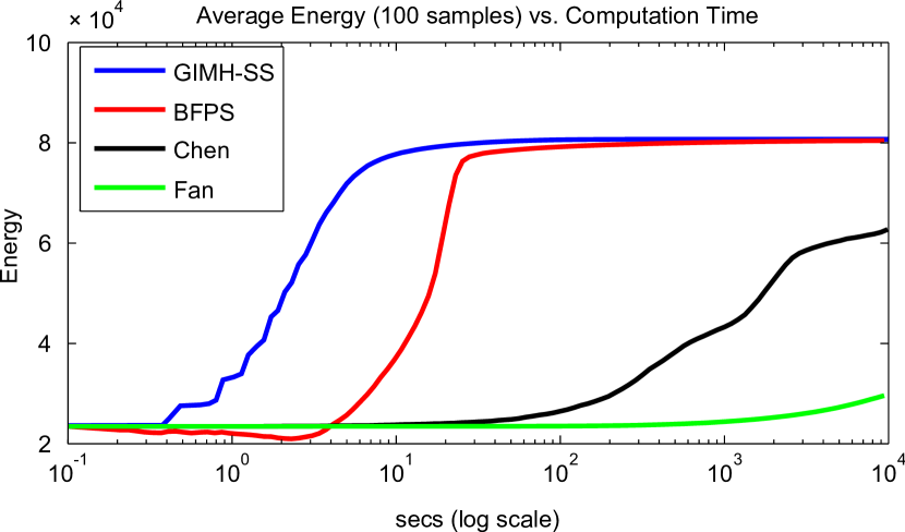
Figure 5: Average energy across 100 sample paths for various shape sampling algorithms. Original image shown on the left.

These results combined with those found in [1] indicate that GIMH-SS draws samples approximately $10$x faster than BFPS, $10^{5}$x faster than [8], and $10^{6}$x faster than [7].

3.3 Relation to Block Gibbs Sampling

Block Gibbs sampling first selects a mask of pixels (or dimensions) to changes, and then samples from the target distribution conditioned on all other pixels. In binary segmentation, a block of size $\left|m\right|$ would require one to evaluate an exponential number ($2^{\left|m\right|}$) of different configurations, which is intractable for a reasonably sized mask.

The GIMH-SS algorithm similarly selects a mask of pixels. The level-set function orders the masked pixels, in that, if a pixel of height $+h$ changes sign, all pixels of height $0<\varphi_{i}<h$ must as well. Consequently, this algorithm samples from a subset of the conditional distribution, resulting in a linear number ($\left|m\right|+1$) of different configurations. We note that ergodicity is ensured because the ordering of pixels by the level-set function changes over time.

4 Topology-Controlled Sampling

In this section, we extend GIMH-SS to a topology-controlled sampler. The topology of a continuous, compact surface is often described by its genus (i.e. the number of “handles”). Digital topology [11] is the discrete counterpart of continuous topology, where regions are represented via binary variables on a grid.

In digital topology, connectiveness must be defined for the foreground (FG) and background (BG) describing how pixels in a local neighborhood are connected. For example, in 2D, a 4-connected region corresponds to a pixel being connected to its neighbors above, below, left, and right. An 8-connected region corresponds to being connected to the eight pixels in a 3x3 neighborhood. Connectiveness must be jointly defined for the foreground ($n$) and background ($\overline{n}$) to avoid topological paradoxes. As shown in [11], valid connectivities for 2D are $(n,\overline{n})\in\left\{(4,8),(8,4)\right\}$. Given a pair of connectiveness, the topological numbers [12] at a particular pixel, $T_{n}$ (for the FG) and $T_{\overline{n}}$ (for the BG) count the number of connected components a pixel is connected to in a 3x3 neighborhood. Figure 6 shows a few neighborhoods with their corresponding topological numbers.

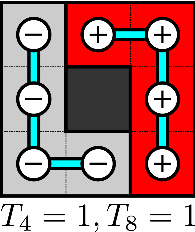
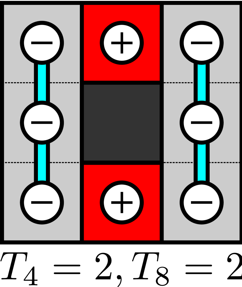
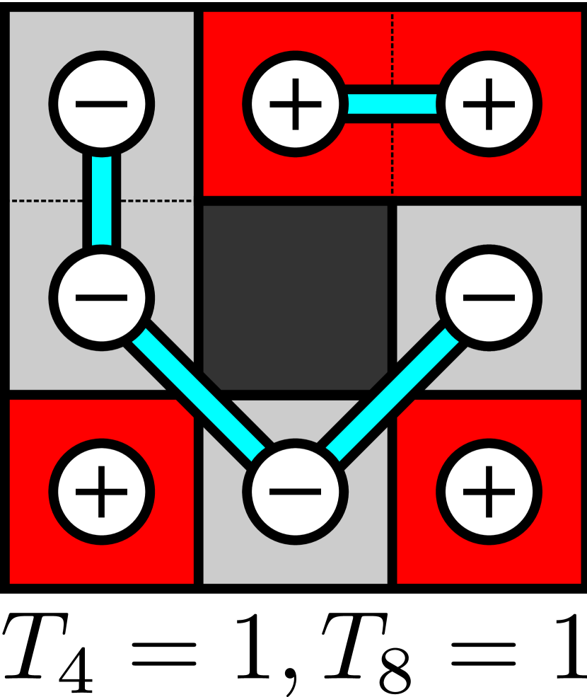
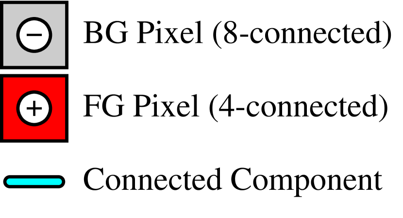
Figure 6: Examples of topological numbers with $(n,\overline{n})=(4,8)$.

While these topological numbers reflect topological changes, they do not distinguish splitting or merging of regions from the creation or destruction of a handle. Segonne [6] defines two additional topological numbers, $T_{n}^{+}$ and $T_{\overline{n}}^{+}$, which count the number of unique connected components a pixel is connected to over the entire image domain. $T_{n}^{+}$ and $T_{\overline{n}}^{+}$ depend on how pixels are connected outside of the 3x3 region and allow one to distinguish all topological changes.

By labeling each connected component in the foreground and background, Segonne shows that $T_{n}^{+}$ can be computed efficiently when a pixel is added to the foreground and $T_{\overline{n}}^{+}$ when a pixel is added to the background. In 3D, one must calculate $T_{\overline{n}}^{+}$ when adding a pixel to the foreground, which can be computationally expensive. We show here that this calculation is not necessary in 2D.

Consider the two pixels marked by $\circ$ and $\triangle$ in Figure 7.

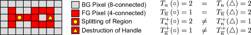
Figure 7: Splitting a region vs. destroying a handle while a pixel is added to BG. Topologal numbers are shown on right.

Removing the $\circ$ pixel from the foreground splits the region and removing the $\triangle$ pixel destroys a handle. We emphasize that in this 2D case, both $T_{n}^{+}(\circ)\neq T_{n}^{+}(\triangle)$ and $T_{\overline{n}}^{+}(\circ)\neq T_{\overline{n}}^{+}(\triangle)$. In 3D, this is generally not the case because for the $\triangle$ pixel, the two background regions can actually be connected in another 2D slice of the volume. In fact, in 2D, the destruction of a handle in the foreground corresponds directly to a merging of regions in the background. Likewise, the splitting of regions in the foreground corresponds directly to a creation of a handle in the background. Because of this one-to-one mapping, we do not need to compute the expensive $T_{\overline{n}}^{+}$ when adding a pixel to the foreground. Table 1 summarizes the topological changes of the foreground and background in 2D as a function of the four topological numbers.

				Add to FG		Add to BG
$T_{n}$	$T_{n}^{+}$	$T_{\overline{n}}$	$T_{\overline{n}}^{+}$	FG	BG	FG	BG
0	0	1	1	CR	CH	DR	DH
1	1	0	0	DH	DR	CH	CR
1	1	1	1	-	-	-	-
$\geq 2$	$<T_{n}$	X	X	CH	SR	X	X
$\geq 2$	$\geq 2$	X	X	MR	DH	X	X
X	X	$\geq 2$	$<T_{\overline{n}}$	X	X	SR	CH
X	X	$\geq 2$	$\geq 2$	X	X	DH	MR

Table 1: Topological changes as a function of topological numbers. ‘C’ - Create; ‘D’ - Destroy; ‘S’ - Split; ‘M’ - Merge; ‘H’ - Handle(s); ‘R’ - Region(s); ‘X’ - any value; ‘-’ - no topological change. Omitted configurations are impossible in 2D.

4.1 Topology-Controlled GIMH-SS

In this section, we summarize how to sample from the space of segmentations while enforcing topology constraints (c.f. [Chang2012tech] for details). While the goal is similar to [6], a simple alteration of the level-set velocity in an MCMC framework will not preserve detailed balance. A naïve approach generates proposals using GIMH-SS and rejects samples that violate topology constraints. Such an approach wastes significant computation generating samples that are rejected due to their topology. We take a different approach: only generate proposed samples from the set of allowable topological changes. Recalling the discussion of ranges in GIMH-SS, one can determine which ranges correspond to allowable topologies and which do not. Ranges corresponding to restricted topologies have their likelihood set to zero in a topology-controlled version of GIMH-SS (TC-GIMH-SS). The methodology presented here treats the topology as a hard constraint. A distribution over topologies could be implemented by weighting ranges based on topologies rather than eliminating restricted ones.

Similar to GIMH-SS, TC-GIMH-SS also makes two passes to calculate the likelihoods of the ranges. Starting at $r_{0}$, we either proceed in the positive or negative direction. Because $r_{0}$ corresponds to the range that does not change the sign of any pixels, $r_{0}$ will never correspond to a topological change. As the algorithm iterates through the possible ranges, a list of pixels that violate a topological constraint is maintained. If this violated list is empty after a range is considered, then the range corresponds to an allowable topology. At each iteration, while any pixel in the violated list is allowed to change sign, it is removed and all neighboring pixels in the violated list are checked again as their topological constraint may have changed. In this process, for each range, one must maintain the labels of each connected component.

5 Results

While TC-GIMH-SS applies to almost any PDE-based or graph-based energy functional, we make a specific choice for demonstration purposes. Similar to [10], we learn nonparametric probability densities over intensities and combine mutual information with a curve length penalty. We impose four different topology constraints on the foreground: unconstrained (GIMH-SS), topology-preserving (TP), genus-preserving (GP), and connected-component-preserving (CCP). The TP sampler does not allow any topology changes, the GP sampler only allows the splitting and merging of regions, and the CCP sampler only allows the creation and destruction of handles. Typical samples from each of these constraints are shown in Figure 8. When the topology constraint is incorrect for the object (e.g. using TP or GP), the resulting sample may be undesirable (e.g. creating an isthmus connecting the two connected components of the background). When the topology is correct, however, more robust results can be obtained. For example, the CCP constraint removes some noise in the background.

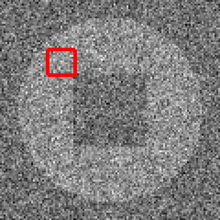
Initialization

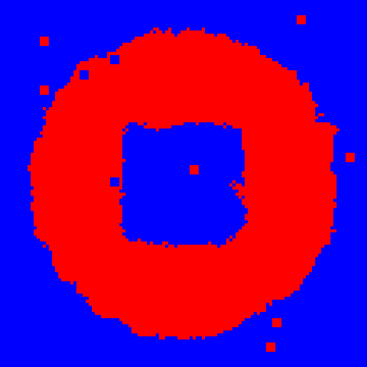
GIMH-SS

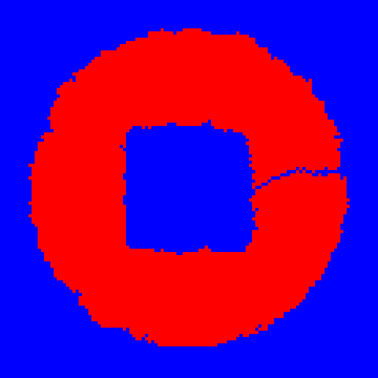
TP

GP

CCP

Figure 8: Example samples imposing different topology constraints.

The usefulness of the topology constraint relies on a valid initialization. Histogram images [7] display the marginal probability that a pixel belongs to the foreground or background where lighter colors equate to higher foreground likelihood. The computed histogram images are shown in Figure 9 for each of the topology constraints.

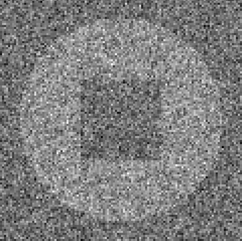
Original

FG Init

Random Init

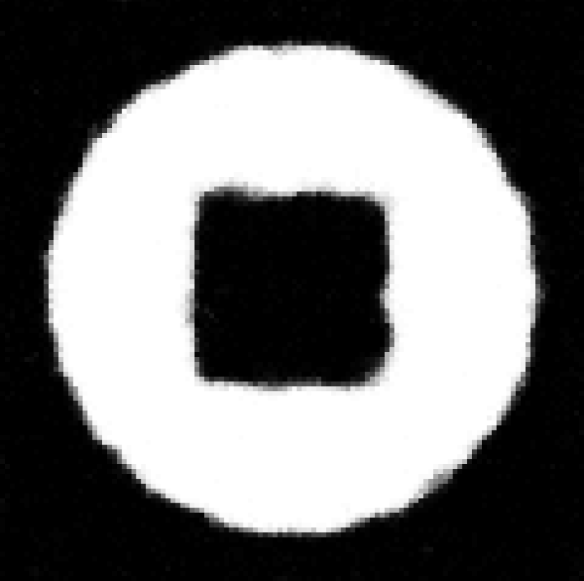
GIMH-SS

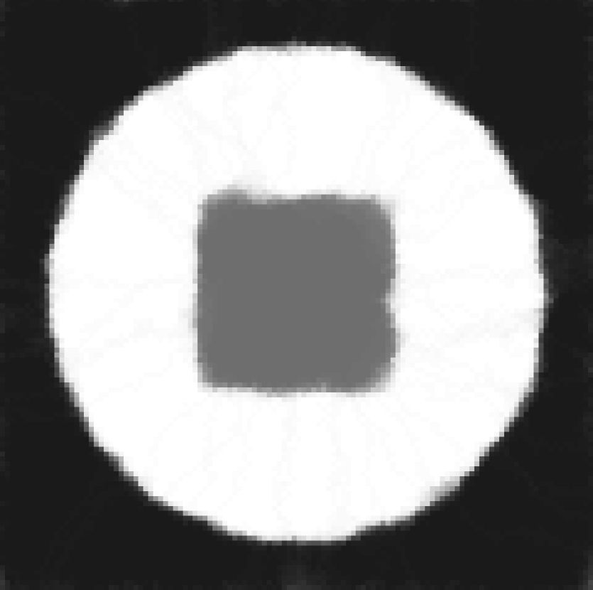
TP

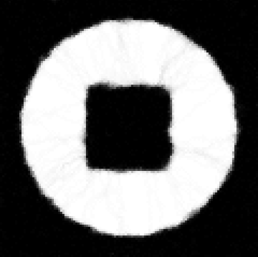
GP

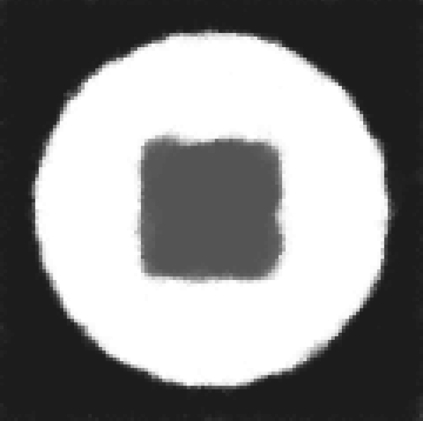
CCP

Figure 9: Histogram images using different initializations.

We initialize the samples either using a random circle containing the foreground (FG Init), or a random circle placed anywhere in the image (Random Init). While not always true, incorrect topology constraints are sometimes mitigated when looking at marginal statistics. For example, in the FG initialization case, the isthmus in the TP and GP constraints is no longer visible. Additionally, if the initialization only captures one connected component of the background (which is possible with random initialization), certain samplers prohibiting splitting regions (TP and CCP) will not be able to capture the entire region. This is reflected in the histogram image with the gray center.

Consider the low SNR image of Figure 10. Chang et al [1] demonstrated that sampling improves results when compared to optimization based methods in low SNR cases. When the problem is less likelihood dominated, as in this case, the prior has greater impact. The top row of Figure 10 shows the histogram images obtained using each of the topological constraints. One can see remnants of the isthmuses in the TP and GP cases.

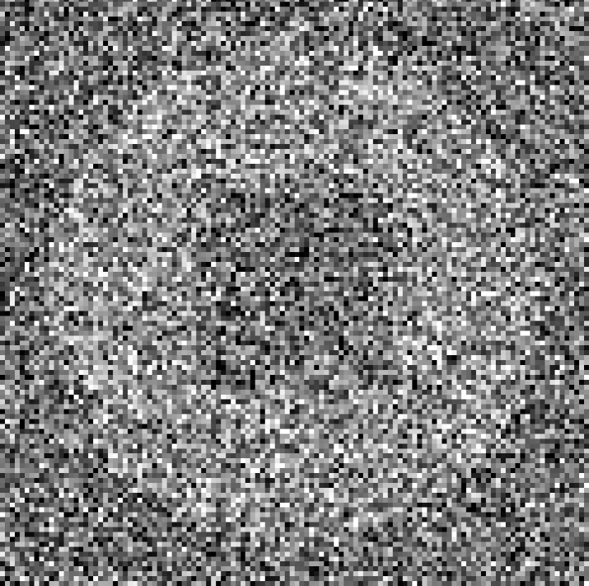
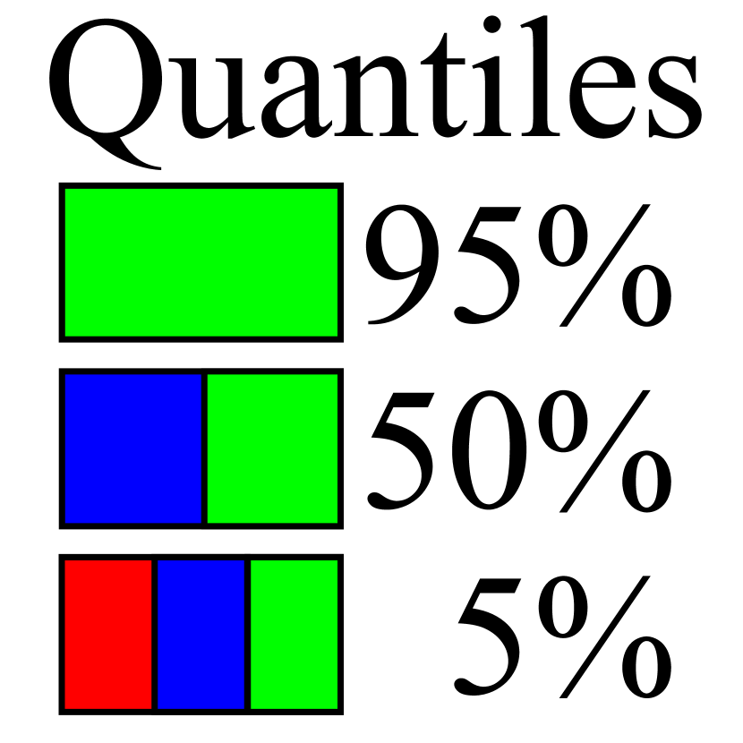
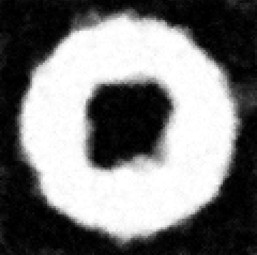
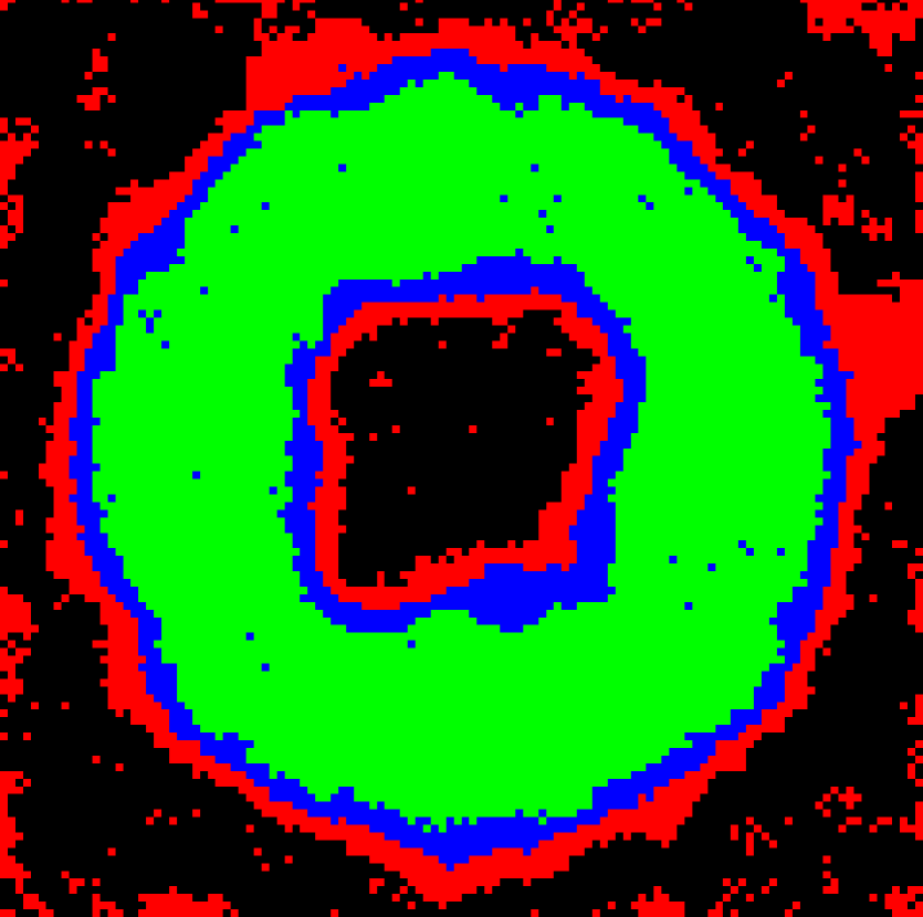
GIMH-SS

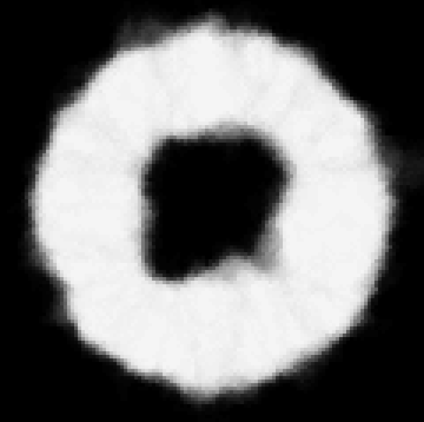
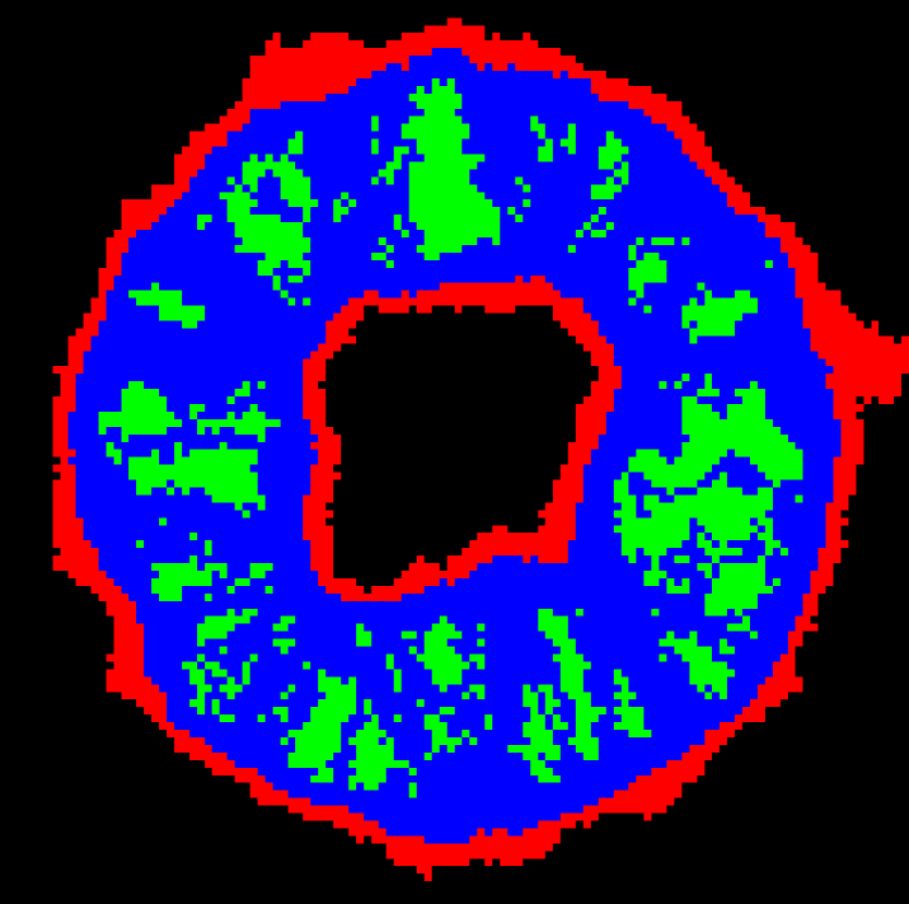
TP

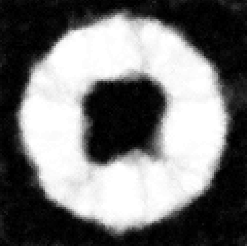
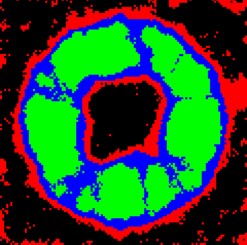
GP

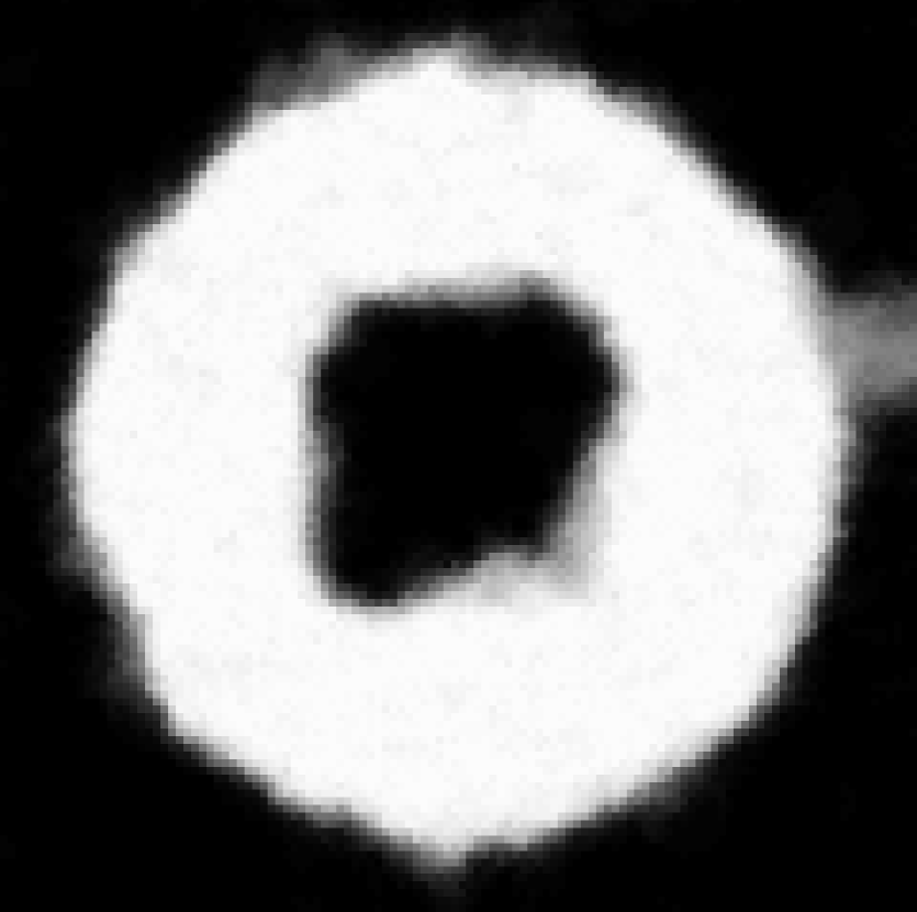
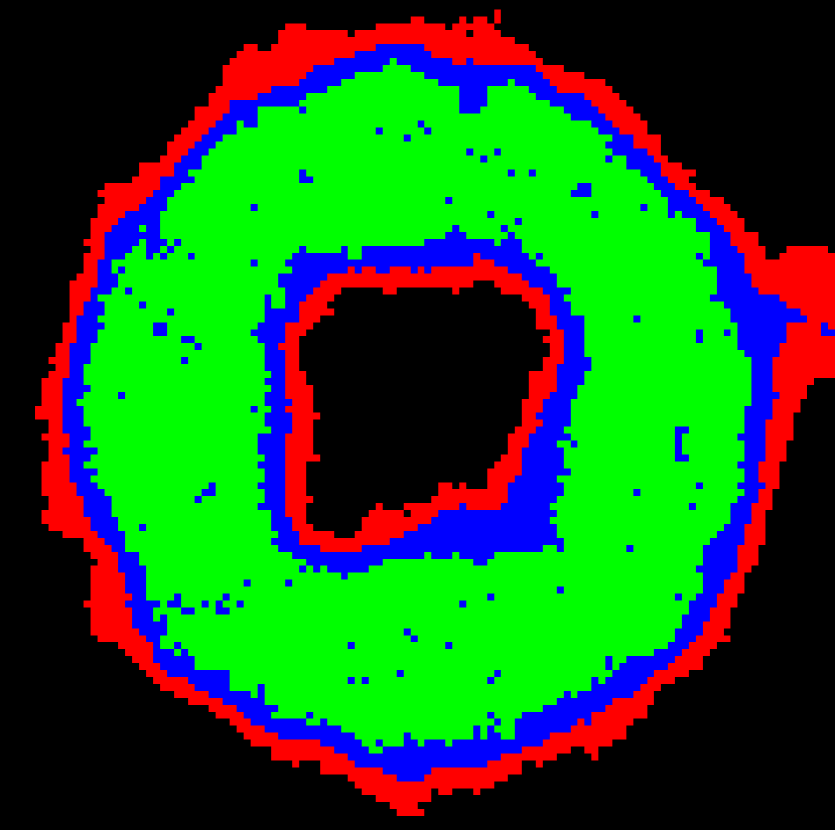
CCP

Figure 10: Low SNR image using FG Init. Histograms are shown above, and quantiles (thresholded histograms) are shown below.

Thresholding the normalized histogram image at a value $t$ reveals the $t^{\text{th}}$ quantile of the segmentation. For example, if $t=0.9$, the resulting foreground region of the thresholded histogram contains pixels that are in the foreground for at least 90% of the samples. We show the 95%, 50%, and 5% quantile segmentations in Figure 10. Since reducing the threshold never shrinks the foreground segmentation, we can overlay these quantiles on top of each other. In the 5% quantile, we can clearly see the isthmuses in the TP and GP cases. This result is poor because the wrong topology (i.e. the wrong prior) was used. However, if we use the CCP constraint, we are able to improve results as compared to the unconstrained case by removing a lot of the background noise.

The CCP constraint is particularly useful when an unknown number of handles exist (e.g. deformable objects). Objects with a known number of handles in 3D projected onto a 2D plane can have any number of handles. We show two example images of a human and the resulting thresholded histogram image in Figure 11. In the first image, the handles formed by the arms are not captured well with TP and GP. In the second image, the vignetting causes the unconstrained and the GP to group some background with foreground.

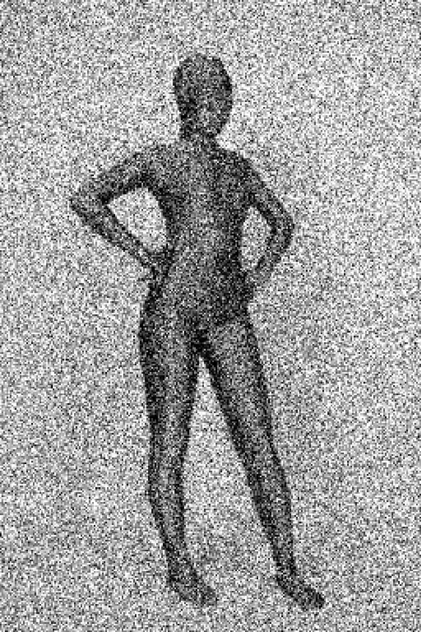
Original

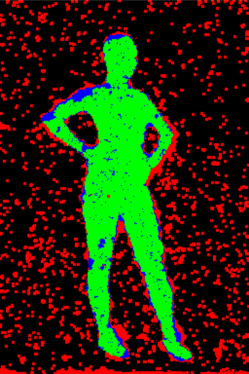
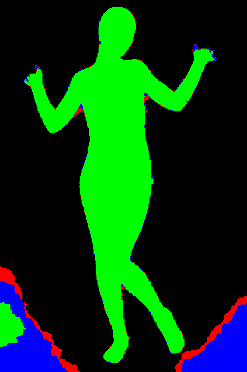
GIMH-SS

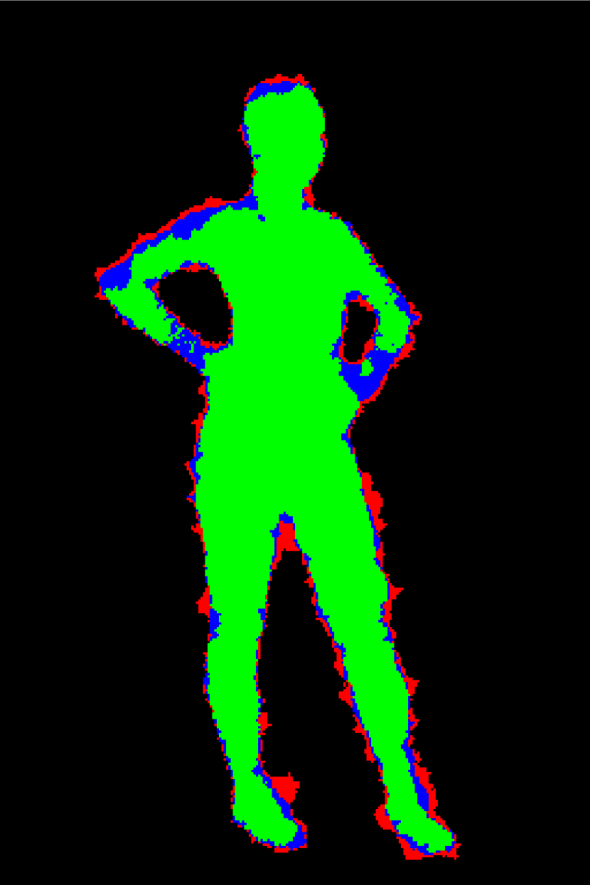
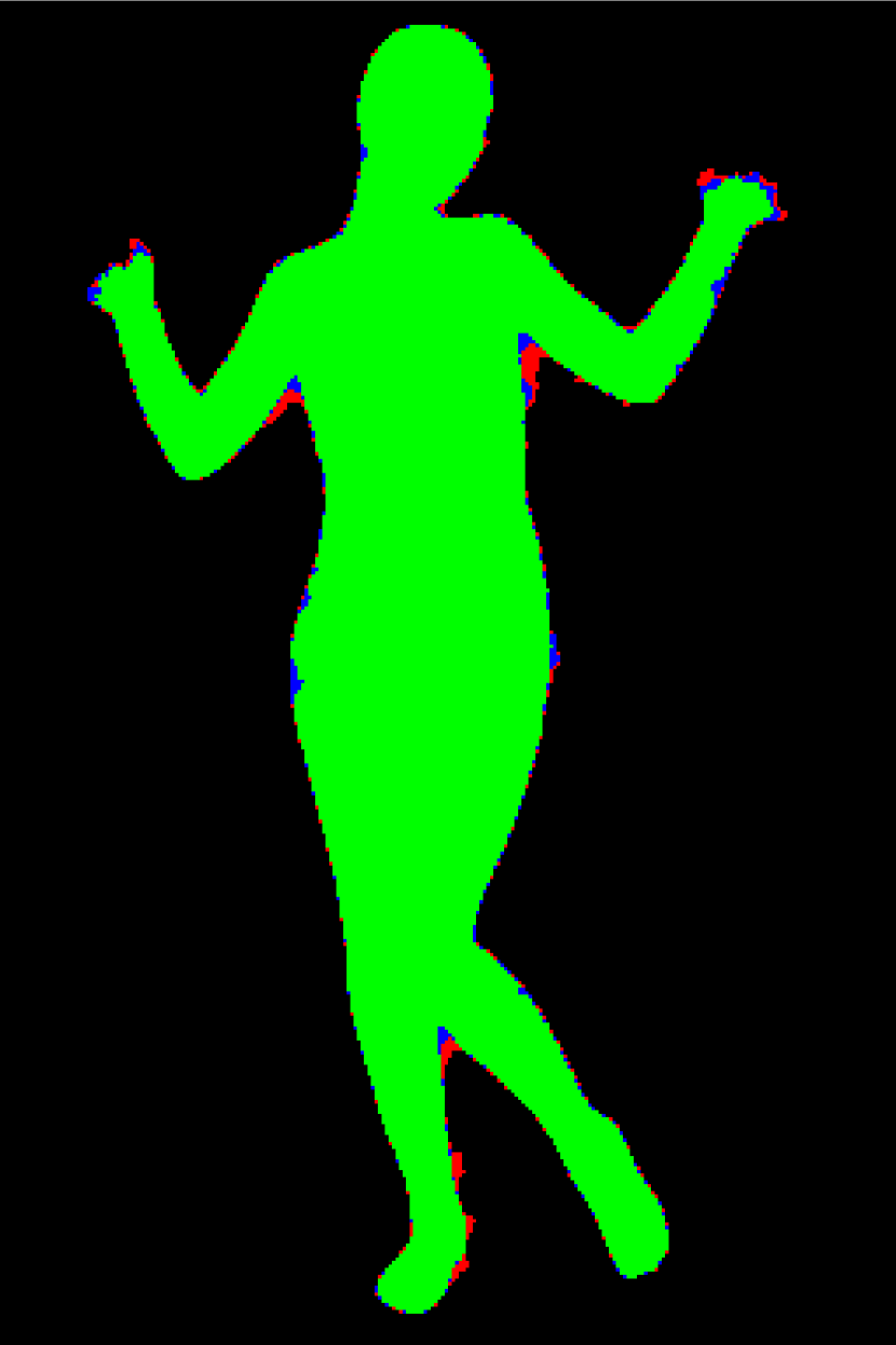
TP

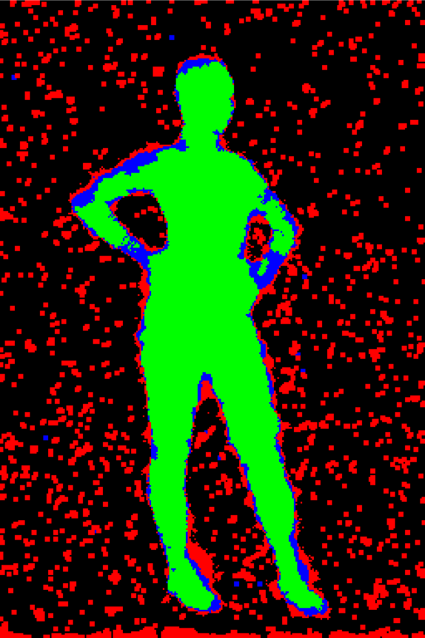
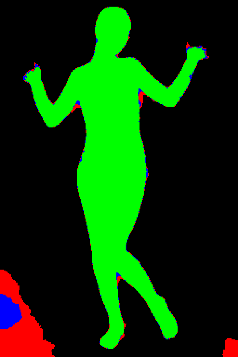
GP

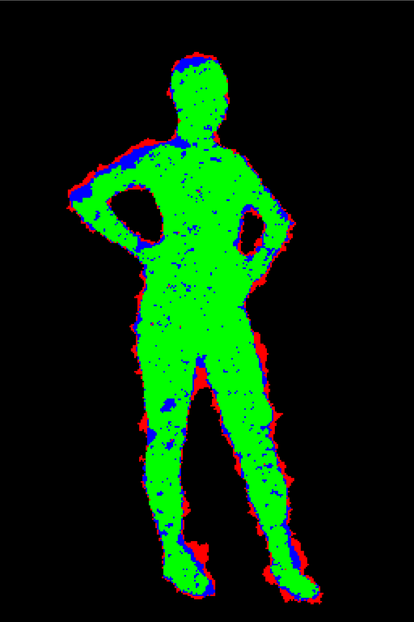
CCP

Figure 11: Example images illustrating the utility of topology priors.

6 Conclusion

We have presented a new MCMC sampler for implicit shapes. We have shown how to design a proposal such that every proposed sample is accepted. Unlike previous methods, GIMH-SS efficiently samples PDE-based and graph-based energy functionals and does not require the evaluation of the gradient of the energy functional (which may be hard to compute). Additionally, GIMH-SS was extended to include hard topological constraints by only proposing samples that are topologically consistent with some prior.

7 Acknowledgements

This research was partially supported by the Air Force Office of Scientific Research under Award No. FA9550-06-1-0324. Any opinions, findings, and conclusions or recommendations expressed in this publication are those of the author(s) and do not necessarily reflect the views of the Air Force.

References

- [1] J. Chang and J. W. Fisher III, “Efficient MCMC Sampling with Implicit Shape Representations,” in IEEE CVPR, 2011, pp. 2081–2088.
- [2] D. M. Greig, B. T. Porteous, and A. H. Seheult, “Exact Maximum A Posteriori Estimation for Binary Images,” Jrnl. of the Royal Statistics Society, vol. 51, pp. 271–279, 1989.
- [3] Y. Boykov, O. Veksler, and R. Zabih, “Fast approximate energy minimization via graph cuts,” IEEE Trans. PAMI, vol. 23, pp. 1222–1239, November 2001.
- [4] J. Shi and J. Malik, “Normalized cuts and image segmentation,” IEEE Trans. PAMI, vol. 22, no. 8, pp. 888–905, 2000.
- [5] X. Han, C. Xu, and J. L. Prince, “A topology preserving level set method for geometric deformable models,” IEEE Trans. PAMI, vol. 25, no. 6, pp. 755–768, 2003.
- [6] F. Ségonne, “Active contours under topology control–genus preserving level sets,” Int. J. Comput. Vision, vol. 79, pp. 107–117, August 2008.
- [7] A. C. Fan, J. W. Fisher III, W. M. Wells, J. J. Levitt, and A. S. Willsky, “MCMC curve sampling for image segmentation.,” MICCAI, vol. 10, no. Pt 2, pp. 477–485, 2007.
- [8] S Chen and R. J. Radke, “Markov chain Monte Carlo shape sampling using level sets,” IEEE ICCV Workshops, pp. 296–303, 2009.
- [9] W. K. Hastings, “Monte Carlo sampling methods using Markov chains and their applications,” Biometrika, vol. 57, no. 1, pp. 97–109, 1970.
- [10] J. Kim, J. W. Fisher III, A. Yezzi, M. Cetin, and A. S. Willsky, “A nonparametric statistical method for image segmentation using information theory and curve evolution.,” IEEE Trans. Image Proc., vol. 14, no. 10, pp. 1486–1502, 2005.
- [11] T. Y. Kong and A. Rosenfeld, “Digital topology: introduction and survey,” Comput. Vision Graph. Image Process., vol. 48, pp. 357–393, December 1989.
- [12] G. Bertrand, “Simple points, topological numbers and geodesic neighborhoods in cubic grids,” Pattern Recogn. Lett., vol. 15, pp. 1003–1011, October 1994.