Chromatic Clustering in High Dimensional Space

Abstract

In this paper, we study a new type of clustering problem, called Chromatic Clustering, in high dimensional space. Chromatic clustering seeks to partition a set of colored points into groups (or clusters) so that no group contains points with the same color and a certain objective function is optimized. In this paper, we consider two variants of the problem, chromatic $k$-means clustering (denoted as $k$-CMeans) and chromatic $k$-medians clustering (denoted as $k$-CMedians), and investigate their hardness and approximation solutions. For $k$-CMeans, we show that the additional coloring constraint destroys several key properties (such as the locality property) used in existing $k$-means techniques (for ordinary points), and significantly complicates the problem. There is no FPTAS for the chromatic clustering problem, even if $k=2$. To overcome the additional difficulty, we develop a standalone result, called Simplex Lemma, which enables us to efficiently approximate the mean point of an unknown point set through a fixed dimensional simplex. A nice feature of the simplex is its independence with the dimensionality of the original space, and thus can be used for problems in very high dimensional space. With the simplex lemma, together with several random sampling techniques, we show that a $(1+\epsilon)$-approximation of $k$-CMeans can be achieved in near linear time through a sphere peeling algorithm. For $k$-CMedians, we show that a similar sphere peeling algorithm exists for achieving constant approximation solutions.

1 Introduction

Clustering is one of the most fundamental problems in computer science and finds applications in many different areas [3, 4, 6, 2, 9, 11, 12, 14, 16, 7, 10]. Most existing clustering techniques assume that the to-be-clustered data items are independent from each other. Thus each data item can “freely” determine its membership within the resulting clusters, without paying attention to the clustering of other data items. In recent years, there are also considerable attentions on clustering dependent data and a number of clustering techniques, such as correlation clustering, point-set clustering, ensemble clustering, and correlation connected clustering, have been developed [4, 7, 9, 11, 10].

In this paper, we consider a new type of clustering problems, called Chromatic Clustering, for dependent data. Roughly speaking, a chromatic clustering problem takes as input a set of colored data items and groups them into clusters, according to certain objective functions, so that no pair of items with the same color are grouped together (such a requirement is called chromatic constraint). Chromatic clustering captures the mutual exclusiveness relationship among data items and is a rather useful model for various applications. Due to the additional chromatic constraint, chromatic clustering is thus expected to simultaneously solve the “coloring” and clustering problems, which significantly complicates the problem. As it will be shown later, the chromatic clustering problem is challenging to solve even for the case that each color is shared only by two data items.

For chromatic clustering, we consider in this paper two variants, Chromatic $k$-means Clustering ($k$-CMeans) and Chromatic $k$-median Clustering ($k$-CMedians), in $\mathbb{R}^{d}$ space, where the dimensionality could be very high and $k$ is a fixed number. In both variants, the input is a set $\mathcal{G}$ of $n$ point-sets $G_{1},\cdots,G_{n}$ with each containing a maximum of $k$ points in $d$-dimensional space, and the objective is to partition all points of $\mathcal{G}$ into $k$ different clusters so that the chromatic constraint is satisfied and the total squared distance (i.e., $k$-CMeans) or total distance (i.e., $k$-CMedians) from each point to the center point (i.e., median or mean point) of its cluster is minimized.

Motivation: The chromatic clustering problem is motivated by several interesting applications. One of them is for determining the topological structure of chromosomes in cell biology [10]. In such applications, a set of 3D probing points (e.g., using BAC probes) is extracted from each homolog of the interested chromosome (see Figure 6 in Appendix), and the objective is to determine, for each chromosome homolog, the common spatial distribution pattern of the probes among a population of cells. For this purpose, the set of probes from each homolog is converted into a high dimensional feature point in the feature space, where each dimension represents the distance between a particular pair of probes. Since each chromosome has two (or more as in cancer cells) homologs, each cell contributes $k$ (i.e., two or more) feature points. Due to technical limitation, it is impossible to identify the same homolog from all cells. Thus, the $k$ feature points from each cell form a point-set with the same color (meaning that they are undistinguishable). To solve the problem, one could chromatically cluster all point-sets into $k$ clusters (after normalizing the cell size), with each corresponding to a homolog, and use the mean or median point of each cluster as its common pattern.

Related works: As its generalization, chromatic clustering is naturally related to the traditional clustering problem. Due to the additional chromatic constraint, chromatic clustering could behave quite differently from its counterpart. For example, the $k$-means algorithms in [6, 15] relies on the fact that all input points in a Voronoi cell of the optimal $k$ mean points belong to the same cluster. However, such a key locality property no longer holds for the $k$-CMeans problem.

Chromatic clustering falls in the umbrella of clustering with constraint. For such type of clustering, several solutions exist for some variants [5]. Unfortunately, due to their heuristic nature, none of them can yield quality guaranteed solutions for the chromatic clustering problem. The first quality guaranteed solution for chromatic clustering was obtained recently by Ding and Xu. In [10], they considered a special chromatic clustering problem, where every point-set has exactly $k$ points in the first quadrant, and the objective is to cluster points by cones apexed at the origin, and presented the first PTAS for constant $k$. The $k$-CMeans and $k$-CMedians problems considered in this paper are the general cases of the chromatic clustering problem. Very recently, Arkin et al. [1] considered a chromatic 2D $2$-center clustering problem and presented both approximation and exact solutions.

1.1 Main Results and Techniques

In this paper, we present three main results, a constant approximation and a $(1+\epsilon)$-approximation for $k$-CMeans and their extensions to $k$-CMedians.

• Constant approximation: We show that given any $c$-approximation for $k$-means clustering, it could yield a $(2ck^{2}+2k-1)$-approximation for $k$-CMeans. This not only provides a way for us to generate an initial constant approximation solution for $k$-CMeans through some $k$-means algorithm, but more importantly reveals the intrinsic connection between the two clustering problems.

• $(1+\epsilon)$-approximation: We show that a near linear time $(1+\epsilon)$-approximation solution for $k$-CMeans can be obtained using an interesting sphere peeling algorithm. Due to the lack of locality property in $k$-CMeans, our sphere peeling algorithm is quite different from the ones used in [15, 6], which in general do not guarantee a $(1+\epsilon)$-approximation solution for $k$-CMeans as shown by our first result. Our sphere peeling algorithm is based on another standalone result, called Simplex Lemma. The simplex lemma enables us to obtain an approximate mean point of a set of unknown points through a grid inside a simplex determined by some partial knowledge of the unknown point set. A unique feature of the simplex lemma is that the complexity of the grid is independent of the dimensionality, and thus can be used to solve problems in high dimensional space. With the simplex lemma, our sphere peeling algorithm iteratively generates the mean points of $k$-CMeans with each iteration building a simplex for the mean point.

• Extensions to $k$-CMedians: We further extend the idea for $k$-CMeans to $k$-CMedians. Particularly, we show that any $c$-approximation for $k$-medians can be used to yield a $((2+\epsilon)ck^{2}+(2+\epsilon)k+1)$-approximation for $k$-CMedians, where the $\epsilon$ error comes from the difficulty of computing the optimal median point (i.e., Fermat Weber point). With this and a similar sphere peeling technique, we obtain a $(5+\epsilon)$-approximation for $k$-CMedians. Note that although $k\geq 2$ is a constant in this paper, a $(5+\epsilon)$-approximation is still much better than a $((2+\epsilon)ck^{2}+(2+\epsilon)k+1)$-approximation.

Due to space limit, many details of our algorithms, proofs, and figures are put in Appendix.

2 Preliminaries

In this section, we introduce some definitions which will be used throughout the paper.

Definition 1 (Chromatic Partition)

Let $\mathcal{G}=\{G_{1},\cdots,G_{n}\}$ be a set of $n$ point-sets with each $G_{i}=\{p^{i}_{1},\dots,p^{i}_{k_{i}}\}$ consisting of $k_{i}\leq k$ points in $\mathbb{R}^{d}$ space. A chromatic partition of $\mathcal{G}$ is a partition of the $\sum_{1\leq i\leq n}k_{i}$ points into $k$ sets, $U_{1},\cdots,U_{k}$, such that each $U_{i}$ contains no more than one point from each $G_{j}$ for $j=1,2,\cdots,n$.

Definition 2 (Chromatic $k$-means Clustering ($k$-CMeans))

Let $\mathcal{G}=\{G_{1},\cdots,$ $G_{n}\}$ be a set of $n$ point-sets with each $G_{i}=\{p^{i}_{1},\dots,p^{i}_{k_{i}}\}$ consisting of $k_{i}\leq k$ points in $\mathbb{R}^{d}$ space. The chromatic $k$-means clustering (or $k$-CMeans) of $\mathcal{G}$ is to find $k$ points $\{m_{1},\cdots,m_{k}\}$ in $\mathbb{R}^{d}$ space and a chromatic partition $U_{1},\cdots,U_{k}$ of $\mathcal{G}$ such that $\frac{1}{n}\sum_{j}\sum_{q\in U_{j}}||q-m_{j}||^{2}$ is minimized. The problem is called full $k$-CMeans if $k_{1}=k_{2}=\cdots=k_{n}=k$.

For both $k$-CMedians and $k$-CMeans, a problem often encountered in our approach is “How to find the best cluster for each point in $G_{i}$ if the $k$ mean or median points $A=\{m_{1},\cdots,m_{k}\}$ are already known?” An easy way to solve this problem is to first build a complete bipartite graph $(G_{i}\cup A,E_{i})$ with points in $G_{i}$ and $A$ as the two partites and then compute a minimum weight bipartite matching as the solution, where the edge weight is the Euclidean distance or squared distance of the two corresponding vertices. Clearly, this can be done in a total of $O(k^{3}dn)$ time for all $G_{i}$’s. (We call this procedure as bipartite matching.)

3 Hardness of $k$-CMeans

It is easy to see that $k$-means is a special case of $k$-CMeans (i.e., each $G_{i}$ contains exactly one point). As shown by Dasgupta [8], $k$-means in high dimensional space is NP-hard even if $k=2$. Thus, we immediately have the following theorem.

Theorem 3.1

$k$-CMeans is NP-hard for $k\geq 2$ in high dimensional space.

3.1 Is Full $k$-CMeans Easier?

It is interesting to know whether full $k$-CMeans is easier than general $k$-CMeans, since it is disjoint with $k$-means when $k\geq 2$. The following theorem gives a negative answer to this question.

Theorem 3.2

Full $k$-CMeans is NP-hard and has no FPTAS for $k\geq 2$ in high dimensional space unless P=NP (see Appendix for the proof).

The above theorem indicates that the fullness of $k$-CMeans does not reduce the hardness of the problem. However, this does not necessarily mean that full $k$-CMeans is as difficult as general $k$-CMeans to achieve a $(1+\epsilon)$-approximation for fixed $k$. Below we show that a $(1+\epsilon)$-approximation can be relatively easily achieved for full $k$-CMeans through some random sampling technique.

First we introduce a key lemma from [13]. Let $S$ be a set of $n$ points in $\mathbb{R}^{d}$ space, $T$ be a randomly selected subset from $S$ with $t$ points, and $\overline{x}(S)$, $\overline{x}(T)$ be the mean points of $S$ and $T$ respectively.

Lemma 1 ([13])

With probability $1-\eta$, $||\overline{x}(S)-\overline{x}(T)||^{2}<\frac{1}{\eta t}Var^{0}(S)$, where $Var^{0}(S)$ $=(\sum_{s\in S}||s-\overline{x}(S)||^{2})/n$.

Lemma 2

Let $S$ be a set of elements, and $S^{\prime}$ be a subset of $S$ such that $\frac{|S^{\prime}|}{|S|}=\alpha$. If randomly select $\frac{t\ln\frac{t}{\eta}}{\ln(1+\alpha)}=O(\frac{t}{\alpha}\ln\frac{t}{\eta})$ elements from $S$, with probability at least $1-\eta$, the sample contains at least $t$ elements from $S^{\prime}$.

Proof

If we randomly select $z$ elements from $S$, then it is easy to know that with probability $1-(1-\alpha)^{z}$, there is at least one element from the sample belonging to $S^{\prime}$. If we want the probability $1-(1-\alpha)^{z}$ equal to $1-\eta/t$, $z$ has to be $\frac{\ln\frac{t}{\eta}}{\ln\frac{1}{1-\alpha}}=\frac{\ln\frac{t}{\eta}}{\ln(1+\frac{\alpha}{1-\alpha})}\leq\frac{\ln\frac{t}{\eta}}{\ln(1+\alpha)}=O(\frac{1}{\alpha}\ln\frac{t}{\eta})$ (by Taylor series and $\alpha<1$, $\ln(1+\alpha)=O(\alpha)$). Thus if we perform $t$ rounds of random sampling with each round selecting $O(\frac{1}{\alpha}\ln\frac{t}{\eta})$ elements, we get at least $t$ elements from $S^{\prime}$ with probability at least $(1-\eta/t)^{t}\geq 1-\eta$. ∎

Lemma 1 tells us that if we want to find an approximate mean point within a distance of $\epsilon Var^{0}(S)$ to the mean point, we just need to take a random sample of size $O(1/\epsilon)$. Lemma 2 suggests that for any set $S$ and its subset $S^{\prime}\subset S$ of size $\alpha|S|$, we can have a random subset $T$ of $S^{\prime}$ with size $O(1/\epsilon)$ by randomly sampling directly from $S$ $O(\frac{1}{\epsilon\alpha}\ln\frac{1}{\epsilon})$ points, even if $S^{\prime}$ is an unknown subset of $S$. Combining the two lemmas, we can immediately compute an approximation solution for full $k$-CMeans in the following way. First, we note that in full $k$-CMeans, each optimal cluster contains exact $n$ points from the total of $kn$ points in $\mathcal{G}$. This means that each cluster has a fraction of $\frac{1}{k}$ points from $\mathcal{G}$. Then, we can obtain an approximate mean point for each optimal cluster by (1) randomly sampling $O(\frac{k}{\epsilon}\ln\frac{1}{\epsilon})$ points from $\mathcal{G}$, (2) enumerating all possible subsets of size $O(1/\epsilon)$ to find the set $T$ which is a random sample of the unknown optimal cluster, and (3) computing the mean of $T$ as the approximate mean point of the optimal cluster. Finally, we can generate the $k$ chromatic clusters from the $k$ approximate mean points by using the bipartite matching procedure (see Section 2).

Theorem 3.3

With constant probability, a $(1+\epsilon)$-approximation of full $k$-CMeans can be obtained in $O(2^{poly(\frac{k}{\epsilon})}$ $nd)$ time.

With the above theorem, we only need to focus on the general $k$-CMeans problem in the remaining sections. Note that in the general case, some clusters may have a very small fraction (rather than $1/k$) of points, thus we can not use the above method to solve the general $k$-CMeans problem.

4 Constant Approximation from $k$-means

In this section, we show that a constant approximation solution for $k$-CMeans can be produced from an approximation solution of $k$-means. Below is the main theorem of this section.

Theorem 4.1

Let $\mathcal{G}=\{G_{1},\cdots,G_{n}\}$ be an instance of $k$-CMeans, and $\mathcal{C}$ be the $k$ mean points of a constant $c$-approximation solution of $k$-means on the points $\cup^{n}_{i=1}G_{i}$. Then $[\mathcal{C}]^{k}$ contains at least one $k$-tuple which could induce a $(2ck^{2}+2k-1)$-approximation of $k$-CMeans on $\mathcal{G}$, where $[\mathcal{C}]^{k}=\underbrace{\mathcal{C}\times\cdots\times\mathcal{C}}_{k}$.

To prove Theorem 4.1, we first introduce two lemmas.

Lemma 3

Let $P$ be a set of points in $\mathbb{R}^{d}$ space, and $m$ be the mean point of $P$. For any point $m^{\prime}\in\mathbb{R}^{d}$, $\sum_{p\in P}||p-m^{\prime}||^{2}=\sum_{p\in P}||p-m||^{2}+|P|\times||m-m^{\prime}||^{2}$ (see Appendix for the proof).

Lemma 4

Let $P$ be a set of points in $\mathbb{R}^{d}$ space, and $P_{1}$ be its subset containing $\alpha|P|$ points for some $0<\alpha\leq 1$. Let $m$ and $m_{1}$ be the mean points of $P$ and $P_{1}$ respectively. Then $||m_{1}-m||\leq\sqrt{\frac{1-\alpha}{\alpha}}\delta$, where $\delta^{2}=\frac{1}{|P|}\sum_{p\in P}||p-m||^{2}$.

Proof

Let $P_{2}=P\setminus P_{1}$, and $m_{2}$ be its mean point. By Lemma 3 we first have the following two equalities.

$$\sum_{p\in P_{1}}||p-m||^{2} = \sum_{p\in P_{1}}||p-m_{1}||^{2}+|P_{1}|\times||m_{1}-m||^{2}.$$ (1)

$$\sum_{p\in P_{2}}||p-m||^{2} = \sum_{p\in P_{2}}||p-m_{2}||^{2}+|P_{2}|\times||m_{2}-m||^{2}.$$ (2)

Then by the definition of $\delta$, we have $\delta^{2}=\frac{1}{|P|}(\sum_{p\in P_{1}}||p-m||^{2}+\sum_{p\in P_{2}}||p-m||^{2})$. Let $L=||m_{1}-m_{2}||$. By the definition of mean point, we have $m=\frac{1}{|P|}\sum_{p\in P}p=\frac{1}{|P|}(\sum_{p\in P_{1}}p+\sum_{p\in P_{2}}p)=\frac{1}{|P|}(|P_{1}|m_{1}+|P_{2}|m_{2})$. Thus the three points $\{m,m_{1},m_{2}\}$ are collinear, and $||m_{1}-m||=(1-\alpha)L$ and $||m_{2}-m||=\alpha L$. Combining (1) and (2), we have

$$\delta^{2}=\frac{1}{|P|}(\sum_{p\in P_{1}}||p-m_{1}||^{2}+|P_{1}|\times||m_{1}-m||^{2}+\sum_{p\in P_{2}}||p-m_{2}||^{2}+|P_{2}|\times||m_{2}-m||^{2})$$

$$\geq\frac{1}{|P|}(|P_{1}|\times||m_{1}-m||^{2}+|P_{2}|\times||m_{2}-m||^{2})=\alpha((1-\alpha)L)^{2}+(1-\alpha)(\alpha L)^{2}=\alpha(1-\alpha)L.$$

Thus, we have $L\leq\frac{\delta}{\sqrt{\alpha(1-\alpha)}}$, which means that $||m_{1}-m||=(1-\alpha)L\leq\sqrt{\frac{1-\alpha}{\alpha}}\delta$. ∎

Proof (of Theorem 4.1)

Let $\{c_{1},\cdots,c_{k}\}$ be the $k$ mean points in $\mathcal{C}$, and $\{S_{1},\cdots,S_{k}\}$ be their corresponding clusters. Let $\{m_{1},\cdots,m_{k}\}$ be the $k$ unknown optimal mean points of $k$-CMeans, and $\mathcal{OPT}=\{Opt_{1},\cdots,Opt_{k}\}$ be the corresponding $k$ optimal chromatic clusters. Let $\Gamma^{i}_{j}=Opt_{i}\cap S_{j}$, and $\tau^{i}_{j}$ be its mean point for $1\leq i,j\leq k$.

Figure 1: An example illustrating Theorem 4.1.

Since $\cup^{k}_{j=1}\Gamma^{i}_{j}=Opt_{i}$, by pigeonhole principle we know that there must exist some index $1\leq j_{i}\leq k$ such that $|\Gamma^{i}_{j_{i}}|\geq\frac{1}{k}|Opt_{i}|$. Thus by fixing $j_{i}$, we have the following about $\sum_{p\in Opt_{i}}||p-c_{j_{i}}||^{2}$ (see Figure 1)

$$\sum_{p\in Opt_{i}}||p-c_{j_{i}}||^{2} = \sum_{p\in Opt_{i}}||p-m_{i}||^{2}+|Opt_{i}|\times||m_{i}-c_{j_{i}}||^{2}=\sum_{p\in Opt_{i}}||p-m_{i}||^{2}+|Opt_{i}|\times||m_{i}-\tau^{i}_{j_{i}}+\tau^{i}_{j_{i}}-c_{j_{i}}||^{2}$$ (3)

$$\leq \sum_{p\in Opt_{i}}||p-m_{i}||^{2}+|Opt_{i}|\times(||m_{i}-\tau^{i}_{j_{i}}||+||\tau^{i}_{j_{i}}-c_{j_{i}}||)^{2}$$

$$\leq \sum_{p\in Opt_{i}}||p-m_{i}||^{2}+|Opt_{i}|\times 2(||m_{i}-\tau^{i}_{j_{i}}||^{2}+||\tau^{i}_{j_{i}}-c_{j_{i}}||^{2}),$$

where the first equation follows from Lemma 3 (note that $m_{i}$ is the mean point of $Opt_{i}$), and the last inequality follows from the fact that $(a+b)^{2}\leq 2(a^{2}+b^{2})$ for any numbers $a$ and $b$. By Lemma 4, we have

$$||\tau^{i}_{j_{i}}-m_{i}||^{2}\leq\frac{1-\frac{1}{k}}{\frac{1}{k}}(\frac{1}{|Opt_{i}|}\sum_{p\in Opt_{i}}||p-m_{i}||^{2}).$$ (4)

$$||\tau^{i}_{j_{i}}-c_{j_{i}}||^{2}\leq\frac{1-\frac{|\Gamma^{i}_{j_{i}}|}{|S_{j_{i}}|}}{\frac{|\Gamma^{i}_{j_{i}}|}{|S_{j_{i}}|}}(\frac{1}{|S_{j_{i}}|}\sum_{p\in S_{j_{i}}}||p-c_{j_{i}}||^{2}).$$ (5)

Plugging (4) and (5) into inequality (3), we have

$$\sum_{p\in Opt_{i}}||p-c_{j_{i}}||^{2}\leq\sum_{p\in Opt_{i}}||p-m_{i}||^{2}+|Opt_{i}|\times 2(||m_{i}-\tau^{i}_{j_{i}}||^{2}+||\tau^{i}_{j_{i}}-c_{j_{i}}||^{2})$$

$$\vspace{-0.05in}\leq\sum_{p\in Opt_{i}}||p-m_{i}||^{2}+|Opt_{i}|\times 2(\frac{1-\frac{1}{k}}{\frac{1}{k}}(\frac{1}{|Opt_{i}|}\sum_{p\in Opt_{i}}||p-m_{i}||^{2})+\frac{1-\frac{|\Gamma^{i}_{j_{i}}|}{|S_{j_{i}}|}}{\frac{|\Gamma^{i}_{j_{i}}|}{|S_{j_{i}}|}}(\frac{1}{|S_{j_{i}}|}\sum_{p\in S_{j_{i}}}||p-c_{j_{i}}||^{2}))$$

$$\vspace{-0.05in}=(2k-1)\sum_{p\in Opt_{i}}||p-m_{i}||^{2}+2\frac{|Opt_{i}|}{|\Gamma^{i}_{j_{i}}|}\times(1-\frac{|\Gamma^{i}_{j_{i}}|}{|S_{j_{i}}|})\sum_{p\in S_{j_{i}}}||p-c_{j_{i}}||^{2}).$$

Since $|\Gamma^{i}_{j_{i}}|\geq\frac{1}{k}|Opt_{i}|$, we have $\frac{|Opt_{i}|}{|\Gamma^{i}_{j_{i}}|}\times(1-\frac{|\Gamma^{i}_{j_{i}}|}{|S_{j_{i}}|})\leq k$. Thus the above inequality becomes

$$\sum_{p\in Opt_{i}}||p-c_{j_{i}}||^{2}\leq(2k-1)\sum_{p\in Opt_{i}}||p-m_{i}||^{2}+2k\sum_{p\in S_{j_{i}}}||p-c_{j_{i}}||^{2}.$$ (6)

Summing both sides of (6) over $i$, we have

$$\sum^{k}_{i=1}\sum_{p\in Opt_{i}}||p-c_{j_{i}}||^{2}\leq(2k-1)\sum^{k}_{i=1}\sum_{p\in Opt_{i}}||p-m_{i}||^{2}+2k\sum^{k}_{i=1}\sum_{p\in S_{j_{i}}}||p-c_{j_{i}}||^{2}$$

$$\leq(2k-1)\sum^{k}_{i=1}\sum_{p\in Opt_{i}}||p-m_{i}||^{2}+2k^{2}\sum^{k}_{j=1}\sum_{p\in S_{j}}||p-c_{j}||^{2},$$ (7)

where the second inequality follows from the inequality $\sum_{p\in S_{j_{i}}}||p-c_{j_{i}}||^{2}\leq\sum^{k}_{j=1}\sum_{p\in S_{j}}||p-c_{j}||^{2}$, which implies that $2k\sum^{k}_{i=1}\sum_{p\in S_{j_{i}}}||p-c_{j_{i}}||^{2}\leq 2k^{2}\sum^{k}_{j=1}\sum_{p\in S_{j}}||p-c_{j}||^{2}$.

It is obvious that the optimal objective value of $k$-means is no larger than that of $k$-CMeans on the same set of points in $\mathcal{G}$. Thus, $\sum^{k}_{j=1}\sum_{p\in S_{j}}||p-c_{j}||^{2}\leq c\sum^{k}_{i=1}\sum_{p\in Opt_{i}}||p-m_{i}||^{2}$. Plugging this inequality into inequality (7), we have

$$\sum^{k}_{i=1}\sum_{p\in Opt_{i}}||p-c_{j_{i}}||^{2}\leq(2ck^{2}+2k-1)\sum^{k}_{i=1}\sum_{p\in Opt_{i}}||p-m_{i}||^{2}.$$

The above inequality means that if we take the $k$-tuple $(c_{j_{1}},\cdots,c_{j_{k}})$ as the $k$ approximate mean points for $k$-CMeans, we have a $(2ck^{2}+2k-1)$-approximation solution, where the $k$ chromatic clusters can be obtained by the bipartite matching procedure. Thus, the theorem is proved. ∎

Running Time: In the above theorem, the bipartite matching procedure takes $O(k^{3}nd)$ time for one $k$-tuple. Since there are in total $O(k^{k})$ such $k$-tuples, the total running time is $O(k^{k+3}nd)$ for computing a $(2ck^{2}+2k-1)$-approximation of $k$-CMeans from a $c$-approximation of $k$-means. As $k$ is assumed to be a constant in this paper, the running time is linear.

5 $(1+\epsilon)$-Approximation Algorithm

This section presents our $(1+\epsilon)$-approximation solution to the $k$-CMeans problem. We first introduce a standalone result, Simplex Lemma, and then use it to achieve a $(1+\epsilon)$-approximation for $k$-CMeans. The main idea of the algorithm is to use a sphere peeling technique to generate the chromatic clusters iteratively, where the Simplex Lemma helps to determine a proper peeling region.

5.1 Simplex Lemma

Simplex Lemma is mainly for approximating the mean point of some unknown points set $P$. The only known information about $P$ is a set $S$ of $j$ points with each of them being an approximate mean point of a subset of $P$. The following Simplex lemmas show that it is possible to construct a simplex of $S$ and find the desired approximate mean point of $P$ inside the simplex.

Figure 2: An example for Lemma 5 with $j=4$.

Figure 3: An example for Lemma 6 with $j=4$.

Lemma 5 (Simplex Lemma i@)

Let $P$ be a set of points in $\mathbb{R}^{d}$ with a partition of $P=\cup^{j}_{l=1}P_{l}$ and $P_{l_{1}}\cap P_{l_{2}}=\emptyset$ for any $l_{1}\neq l_{2}$. Let $o$ be the mean point of $P$, and $o_{l}$ be the mean point of $P_{l}$ for $1\leq l\leq j$. Further, let $\delta^{2}=\frac{1}{|P|}\sum_{p\in P}||p-o||^{2}$, and $V$ be the simplex determined by $\{o_{1},\cdots,o_{j}\}$. Then for any $0<\epsilon\leq 1$, it is possible to construct a grid of size $O((8j/\epsilon)^{j})$ inside $V$ such that at least one grid point $\tau$ satisfies the inequality $||\tau-o||\leq\sqrt{\epsilon}\delta$.

Proof

We will prove this lemma by mathematical induction on $j$.

Base case: For $j=1$, since $P_{1}=P$, $o_{1}=o$. Thus, the simplex $V$ and the grid are all simply the point $o_{1}$. Clearly $\tau=o_{1}$ satisfies the inequality.

Induction step: Assume that the lemma holds for any $j\leq j_{0}$ for some $j_{0}\geq 1$ (i.e., Induction Hypothesis). Now we consider the case of $j=j_{0}+1$. First, we assume that $\frac{|P_{l}|}{|P|}\geq\frac{\epsilon}{4j}$ for each $1\leq l\leq j$. Otherwise, we can reduce the problem to the case of smaller $j$ in the following way. Let $I=\{l|1\leq l\leq j,\frac{|P_{l}|}{|P|}<\frac{\epsilon}{4j}\}$ be the index set of small subsets. Then, $\frac{\sum_{l\in I}|P_{l}|}{|P|}<\frac{\epsilon}{4}$, and $\frac{\sum_{l\not\in I}|P_{l}|}{|P|}\geq 1-\frac{\epsilon}{4}$. By Lemma 4, we know that $||o^{\prime}-o||\leq\sqrt{\frac{\epsilon/4}{1-\epsilon/4}}\delta$, where $o^{\prime}$ is the mean point of $\cup_{l\not\in I}P_{l}$. Let $(\delta^{\prime})^{2}$ be the variance of $\cup_{l\not\in I}P_{l}$. Then, we have $(\delta^{\prime})^{2}\leq\frac{|P|}{|\cup_{l\not\in I}P_{l}|}\delta^{2}\leq\frac{1}{1-\epsilon/4}\delta^{2}$. Thus, if we replace $P$ and $\epsilon$ by $\cup_{l\not\in I}P_{l}$ and $\frac{\epsilon}{16}$ respectively, and find a point $\tau$ such that $||\tau-o^{\prime}||^{2}\leq\frac{\epsilon}{16}(\delta^{\prime})^{2}\leq\frac{\epsilon/16}{1-\epsilon/4}\delta^{2}$, we have $||\tau-o||^{2}\leq(||\tau-o^{\prime}||+||o^{\prime}-o||)^{2}\leq\frac{\frac{9}{16}\epsilon}{1-\epsilon/4}\delta^{2}\leq\epsilon\delta^{2}$ (where the last inequality is due to the fact $\epsilon<1$). This means that we can reduce the problem to a problem with point set $\cup_{l\not\in I}P_{l}$ and a smaller $j$ (i.e., $j-|I|$). By the induction hypothesis, we know that the reduced problem can be solved (note that the simplex would be a subset of $V$ determined by $\{o_{l}\mid 1\leq l\leq j,l\not\in I\}$), and therefore the induction step holds for this case. Thus, in the following discussion, we can assume that $\frac{|P_{l}|}{|P|}\geq\frac{\epsilon}{4j}$ for each $1\leq l\leq j$.

For each $1\leq l\leq j$, since $\frac{|P_{l}|}{|P|}\geq\frac{\epsilon}{4j}$, by Lemma 4, we know that $||o_{l}-o||\leq\sqrt{\frac{1-\frac{\epsilon}{4j}}{\frac{\epsilon}{4j}}}\delta\leq 2\sqrt{\frac{j}{\epsilon}}\delta$. This, together with triangle inequality, implies that for any $1\leq l,l^{\prime}\leq j$, $||o_{l}-o_{l^{\prime}}||\leq||o_{l}-o||+||o_{l^{\prime}}-o||\leq 4\sqrt{\frac{j}{\epsilon}}\delta$. Thus, if we pick any index $l_{0}$, and draw a ball $\mathcal{B}$ centered at $o_{l_{0}}$ and with radius $r=\max_{1\leq l\leq j}\{||o_{l}-o_{l_{0}}||\}\leq 4\sqrt{\frac{j}{\epsilon}}\delta$, the whole simplex $V$ will be inside $\mathcal{B}$. Note that since $o=\sum^{j}_{l=1}\frac{|P_{j}|}{|P|}o_{l}$, $o$ also locates inside $V$. This indicates that we can construct $\mathcal{B}$ in the $j-1$-dimensional space spanned by $\{o_{1},\cdots,o_{j}\}$, rather than the whole $\mathbb{R}^{d}$ space. Also, if we build a grid inside $\mathcal{B}$ with grid length $\frac{\epsilon r}{4j}$, the total number of grid points is no more than $O((\frac{8j}{\epsilon})^{j})$. With this grid, we know that for any point $q$ inside $V$, there exists a grid point $g$ such that $||g-q||\leq\sqrt{j(\frac{\epsilon r}{4j})^{2}}=\frac{\epsilon}{4\sqrt{j}}r\leq\sqrt{\epsilon}\delta$. This means that can find a grid point $\tau$ inside $V$, such that $||\tau-o||^{2}\leq\epsilon\delta^{2}$. Thus, the induction step holds.

With the above base case and induction steps, the lemma holds for any $j\geq 1$. ∎

In the above lemma, we assume that the exact positions of $\{o_{1},\cdots,o_{j}\}$ are known (see Fig. 3). However, in some scenario (e.g., the exact partition of $P$ is not given, as is the case in $k$-CMeans), it is possible that we only know the approximate position of each mean point $o_{i}$ (see Fig. 3). The following lemma shows that an approximate position of $o$ can still be similarly determined.

Lemma 6 (Simplex Lemma ii@)

Let $P$, $o$, $P_{l},o_{l},1\leq l\leq j$, and, $\delta$ be defined as in Lemma 5. Let $\{o^{\prime}_{1},\cdots,o^{\prime}_{j}\}$ be $j$ points in $R^{d}$ such that $||o^{\prime}_{l}-o_{l}||\leq L$ for $1\leq l\leq j$ and $L>0$, and $V^{\prime}$ be the simplex determined by $\{o^{\prime}_{1},\cdots,o^{\prime}_{j}\}$. Then for any $0<\epsilon\leq 1$, it is possible to construct a grid of size $O((8j/\epsilon)^{j})$ inside $V^{\prime}$ such that at least one grid point $\tau$ satisfies the inequality $||\tau-o||\leq\sqrt{\epsilon}\delta+(1+\epsilon)L$.

5.2 Sphere Peeling Algorithm

This section presents a sphere peeling algorithm to achieve a $(1+\epsilon)$-approximation for $k$-CMeans.

Let $\mathcal{G}=\{G_{1},\cdots,G_{n}\}$ be an instance of $k$-CMeans with $k$ (unknown) optimal chromatic clusters $\mathcal{OPT}=\{Opt_{1},\cdots,$ $Opt_{k}\}$, and $m_{j}$ be the mean point of the cluster $Opt_{j}$ for $1\leq j\leq k$. Without loss of generality, we assume that $|Opt_{1}|\geq|Opt_{2}|\geq\cdots\geq|Opt_{k}|$.

Algorithm overview: Our algorithm first computes a constant $C$-approximation solution (by Theorem 4.1) to determine an upper bound $\Delta$ of the optimal objective value $\delta^{2}_{opt}$, and then search for a good approximation of $\delta^{2}_{opt}$ in the interval of $[\Delta/C,\Delta]$. At each search step, our algorithm performs a sphere peeling procedure to iteratively generate $k$ approximate mean points for the chromatic clusters. Initially, the sphere peeling procedure uses random sampling technique (i.e., Lemma 1 and 2) to find an approximate mean point for $Opt_{1}$. At $(j+1)$-th iteration, it already has approximate mean points $\{p_{v_{1}},\cdots,p_{v_{j}}\}$ for $Opt_{1},\cdots,Opt_{j}$ respectively. Then it draws $j$ peeling spheres, $B_{j+1,1},\cdots,B_{j+1,j}$, centered at the $j$ approximate mean points respectively and with a radius determined by the approximation of $\delta_{opt}$. Denote the set of unknown points $Opt_{j+1}\setminus(\cup^{j}_{l=1}B_{j+1,l})$ as $\mathcal{A}$. Our algorithm considers two cases: (a) $|\mathcal{A}|$ is large enough and (b) $|\mathcal{A}|$ is small. For case (a), since $|\mathcal{A}|$ is large enough, we can first use Lemma 2 to find an approximate mean point $m_{\mathcal{A}}$ of $\mathcal{A}$, and then construct a simplex determined by $m_{\mathcal{A}}$ and $\{p_{v_{1}},\cdots,p_{v_{j}}\}$. For case (b), it directly constructs a simplex determined just by $\{p_{v_{1}},\cdots,p_{v_{j}}\}$. For either case, our algorithm builds a grid inside the simplex (i.e., using Lemma 6) to find an approximate mean point for $Opt_{j+1}$ (i.e., $p_{v_{j+1}}$). Repeat the sphere peeling procedure $k$ times to generate the $k$ approximate mean points.

Algorithm $k$-CMeans
Input: $\mathcal{G}=\{G_{1},\cdots,G_{n}\}$, $k\geq 2$, and a small positive value $\epsilon$.
Output: $(1+\epsilon)$-approximation solution for $k$-CMeans on $\mathcal{G}$.

1. Run the PTAS of $k$-means in [15] on $\mathcal{G}$, and let $\Delta$ be the obtained objective value.

2. For $i=1$ to $\frac{2k}{\epsilon}$ do

   1. Set $\delta=\frac{\sqrt{\Delta}}{2k}+i\frac{\epsilon}{2k}\sqrt{\Delta}$, and run the Sphere-Peeling-Tree algorithm.

   2. Let $\mathcal{T}_{i}$ be the output tree.

3. For each path of every $\mathcal{T}_{i}$, use bipartite matching procedure to compute the objective value of $k$-CMeans on $\mathcal{G}$. Output the $k$ points from the path with the smallest objective value.

Algorithm Sphere-Peeling-Tree
Input: $\mathcal{G}$, $k\geq 2$, $\epsilon,\delta>0$.
Output: A tree $\mathcal{T}$ of height $k$ with each node $v$ associating with a point $p_{v}\in\mathbb{R}^{d}$.

1. Initialize $\mathcal{T}$ with a single root node $v$ associating with no point.

2. Recursively grow each node $v$ in the following way

   1. If the height of $v$ is already $k$, then it is a leaf.

   2. Otherwise, let $j$ be the height of $v$. Build the radius candidates set $\mathcal{R}=\cup^{\log(kn)}_{t=0}\{\frac{1+l\frac{\epsilon}{2}}{2(1+\epsilon)}j2^{t/2}\sqrt{\epsilon}\delta\mid 0\leq l\leq 4+\frac{2}{\epsilon}\}$. For each $r\in\mathcal{R}$, do

      1. Let $\{p_{v_{1}},\cdots,p_{v_{j}}\}$ be the $j$ points associated with nodes on the root-to-$v$ path.

      2. For each $p_{v_{l}}$, $1\leq l\leq j$, construct a ball $B_{j+1,l}$ centered at $p_{v_{l}}$ and with radius $r$.

      3. Take a random sample from $\mathcal{G}\setminus\cup^{j}_{l=1}B_{j+1,l}$ with size $m=\frac{8k^{3}}{\epsilon^{9}}\ln\frac{k^{2}}{\epsilon^{6}}$. Compute the mean points of all subset of the sample, and denote them as $\Pi=\{\pi_{1},\cdots,\pi_{2^{m}-1}\}$.

      4. For each $\pi_{i}\in\Pi$, construct the simplex determined by $\{p_{v_{1}},\cdots,p_{v_{j}},\pi_{i}\}$. Also construct the simplex determined by $\{p_{v_{1}},\cdots,p_{v_{j}}\}$. Build a grid inside each simplex with size $O((\frac{32j}{\epsilon^{2}})^{j})$.

      5. In total, there are $2^{m}(\frac{32j}{\epsilon^{2}})^{j}$ grid points inside the $2^{m}$ simplices. For each grid point, add one child to $v$, and associate it with the grid point.

Theorem 5.1

With constant probability, Algorithm $k$-CMeans yields a $(1+\epsilon)$-approximation for $k$-CMeans in $O(2^{poly(\frac{k}{\epsilon})}n(\log n)^{k+1}d)$ time.

5.3 Proof of Theorem 5.1

Let $\beta_{j}=|Opt_{j}|/|\cup_{i=1}^{n}G_{i}|$, and $\delta^{2}_{j}=\frac{1}{|Opt_{j}|}\sum_{p\in Opt_{j}}||p-m_{j}||^{2}$, where $m_{j}$ is the mean point of $Opt_{j}$. Clearly, $\beta_{1}\geq\cdots\geq\beta_{k}$ (by assumption) and $\sum^{k}_{j=1}\beta_{j}=1$. Let $\delta^{2}_{opt}=\sum^{k}_{j=1}\beta_{j}\delta^{2}_{j}$.

We prove Theorem 5.1 by mathematical induction. Instead of directly proving it, we consider the following two lemmas which jointly ensure the correctness of Theorem 5.1.

Lemma 7

Among all the trees generated in Algorithm $k$-CMeans, with constant probability, there exists at least one tree, $\mathcal{T}_{i}$, which has a root-to-leaf path with each node $v_{j}$ at level $j$, $1\leq j\leq k$, on the path associating a point $p_{v_{j}}$ and satisfying the inequality $||p_{v_{j}}-m_{j}||\leq\epsilon\delta_{j}+(1+\epsilon)j\sqrt{\frac{\epsilon}{\beta_{j}}}\delta_{opt}.$

Before proving this lemma, we first show its implication.

Lemma 8

If Lemma 7 is true, Algorithm $k$-CMeans yields a $(1+O(k^{3})\epsilon)$-approximation for $k$-CMeans.

Proof

We first assume that Lemma 7 is true. Then for each $1\leq j\leq k$, we have

$$\sum_{p\in Opt_{j}}||p-p_{v_{j}}||^{2} = \sum_{p\in Opt_{j}}||p-m_{j}||^{2}+|Opt_{j}|\times||m_{j}-p_{v_{j}}||^{2}\leq\sum_{p\in Opt_{j}}||p-m_{j}||^{2}+|Opt_{j}|\times 2(\epsilon^{2}\delta^{2}_{j}+(1+\epsilon)^{2}j^{2}\frac{\epsilon}{\beta_{j}}\delta^{2}_{opt})$$ (8)

$$= (1+2\epsilon^{2})|Opt_{j}|\delta^{2}_{j}+2(1+\epsilon)^{2}j^{2}\epsilon|\mathcal{G}|\delta^{2}_{opt},$$

where the first equation follows from Lemma 3 (note that $m_{j}$ is the mean point of $Opt_{j}$), the second inequality follows from Lemma 7 and the fact that $(a+b)^{2}\leq 2(a^{2}+b^{2})$ for any two real numbers $a$ and $b$, and the last equality follows from $\frac{|Opt_{j}|}{\beta_{j}}=|\mathcal{G}|$. Summing both sides of (8) over $j$, we have

$$\sum^{k}_{j=1}\sum_{p\in Opt_{j}}||p-p_{v_{j}}||^{2} \leq \sum^{k}_{j=1}((1+2\epsilon^{2})|Opt_{j}|\delta^{2}_{j}+2(1+\epsilon)^{2}j^{2}\epsilon|\mathcal{G}|\delta^{2}_{opt})$$ (9)

$$\leq (1+2\epsilon^{2})\sum^{k}_{j=1}|Opt_{j}|\delta^{2}_{j}+2(1+\epsilon)^{2}k^{3}\epsilon|\mathcal{G}|\delta^{2}_{opt}=(1+O(k^{3})\epsilon)|\mathcal{G}|\delta^{2}_{opt},$$

where the last equation follows from the fact that $\sum^{k}_{j=1}|Opt_{j}|\delta^{2}_{j}=|\mathcal{G}|\delta^{2}_{opt}$. By (9), we know that $\{p_{v_{1}},\cdots,p_{v_{k}}\}$ will induce a $(1+O(k^{3})\epsilon)$-approximation solution for $k$-CMeans via bipartite matching procedure. Since Algorithm $k$-CMeans outputs the best solution generated in all trees, the resulting solution is clearly a $(1+O(k^{3})\epsilon)$-approximation solution. Thus the lemma is true. ∎

The above lemma indicates that if we replace $\epsilon$ by $\frac{\epsilon}{k^{3}}$ in the input of our algorithm, it will result in a $(1+\epsilon)$-approximation solution. This implies that Lemma 7 is indeed sufficient to ensure the correctness of Theorem 5.1 (except for the time complexity). Now we prove Lemma 7.

Proof (of Lemma 7)

Note that $\Delta\leq 4k^{2}\delta^{2}_{opt}$, and we build $\epsilon$-net in $[\frac{\sqrt{\Delta}}{2k},\sqrt{\Delta}]$. Let $\mathcal{T}_{i}$ be the tree generated by Algorithm Sphere-Peeling-Tree and corresponding to the input $\delta\in[\delta_{opt},(1+\epsilon)\delta_{opt}]$. We will focus our discussion on $\mathcal{T}_{i}$, and prove the lemma by mathematical induction on $j$.

Base case: For $j=1$, since $\beta_{1}=\max\{\beta_{j}|1\leq j\leq k\}$, we have $\beta_{1}\geq\frac{1}{k}$. By Lemmas 1 and 2, we can find the approximation mean point through random sampling. Let $p_{v_{1}}$ be the approximation mean point. Clearly, $||p_{v_{1}}-m_{1}||\leq\epsilon\delta_{1}\leq\epsilon\delta_{1}+(1+\epsilon)\sqrt{\frac{\epsilon}{\beta_{1}}}\delta_{opt}$ (By Lemmas 1 and 2).

Induction step: We assume that there is a path in $\mathcal{T}_{i}$ from the root to the $j_{0}$-th level, such that for each $1\leq l\leq j_{0}$, the level-$l$ node $v_{l}$ on the path is associated with a point $p_{v_{l}}$ satisfying the inequality $||p_{v_{l}}-m_{l}||\leq\epsilon\delta_{l}+(1+\epsilon)l\sqrt{\frac{\epsilon}{\beta_{l}}}\delta_{opt}$ (i.e., Induction Hypothesis). Now we consider the case of $j=j_{0}+1$. Below we will show that there is one child of $v_{j-1}$, i.e., $v_{j}$, such that its associated point $p_{v_{l}}$ satisfies the inequality $||p_{v_{j}}-m_{j}||\leq\epsilon\delta_{j}+(1+\epsilon)j\sqrt{\frac{\epsilon}{\beta_{j}}}\delta_{opt}$. First, we have the following claim (see Appendix for the proof).

Claim (1)

In the set of radius candidates built in Algorithm Sphere-Peeling-Tree, there exists one value $r_{j}\in\mathcal{R}$ such that

$$j\sqrt{\frac{\epsilon}{\beta_{j}}}\delta_{opt}\leq r_{j}\leq(1+\frac{\epsilon}{2})j\sqrt{\frac{\epsilon}{\beta_{j}}}\delta_{opt}.$$

Now, we construct the $j-1$ peeling spheres, $\{B_{j,1},\cdots,B_{j,j-1}\}$ (as in Algorithm Sphere-Peeling-Tree). For each $1\leq l\leq j-1$, $B_{j,l}$ is centered at $p_{v_{l}}$ and with radius $r_{j}$. By Markov inequality and induction hypothesis, we have the following claim (see Appendix for the proof).

Claim (2)

For each $1\leq l\leq j-1$, we have $|Opt_{l}\setminus(\bigcup^{j-1}_{w=1}B_{j,w})|\leq\frac{4\beta_{j}|\mathcal{G}|}{\epsilon}$.

Claim 2 shows that $|Opt_{l}\setminus(\bigcup^{j-1}_{w=1}B_{j,w})|$ is bounded for $1\leq l\leq j-1$, which helps us to find the approximate mean point of $Opt_{j}$. Induced by the $j-1$ peeling spheres $\{B_{j,1},\cdots,B_{j,j-1}\}$, $Opt_{j}$ is divided into $j$ subsets, $Opt_{j}\cap B_{j,1}$, $\cdots$, $Opt_{j}\cap B_{j,j-1}$ and $Opt_{j}\setminus(\bigcup^{j-1}_{w=1}B_{j,w})$. To simplify our discussion, we let $P_{l}$ denote $Opt_{j}\cap B_{j,l}$ for $1\leq l\leq j-1$, $P_{j}$ denote $Opt_{j}\setminus(\bigcup^{j-1}_{w=1}B_{j,w})$, and $\tau_{l}$ denote the mean point of $P_{l}$. Note that the peeling spheres may intersect with each other. For any two intersecting spheres $B_{j,l_{1}}$ and $B_{j,l_{2}}$, we let the points set $Opt_{j}\cap(B_{j,l_{1}}\cap B_{j,l_{2}})$ belong to either $P_{l_{1}}$ or $P_{l_{2}}$ arbitrarily. Thus, we can assume that $\{P_{l}\mid 1\leq l\leq j\}$ are pairwise disjoint. Now consider the size of $P_{j}$ (i.e., $|P_{j}|$). We have the following two cases: (a) $|P_{j}|\geq\epsilon^{3}\frac{\beta_{j}}{j}|\mathcal{G}|$ and (b) $|P_{j}|<\epsilon^{3}\frac{\beta_{j}}{j}|\mathcal{G}|$. In the following, we show how, in each case, Algorithm Sphere-Peeling-Tree can obtain an approximate mean point for $Opt_{j}$ by using the Simplex Lemma (i.e., Lemma 6).

Figure 4: Case (a) for $j=4$.

Figure 5: Case (b) for $j=4$.

For case (a), by Claim 2, together with the fact that $\beta_{l}\leq\beta_{j}$ for $l>j$, we know that

$$\frac{|P_{j}|}{\sum_{1\leq i\leq k}|Opt_{i}\setminus(\bigcup^{j-1}_{l=1}B_{j,l})|}\geq\frac{\frac{\epsilon^{3}}{j}\beta_{j}}{\frac{4(j-1)\beta_{j}}{\epsilon}+\frac{\epsilon^{2}}{j}\beta_{j}+(k-j)\beta_{j}}>\frac{\epsilon^{4}}{8kj}\geq\frac{\epsilon^{4}}{8k^{2}}.$$

This means that $P_{j}$ is large enough, comparing to the set of points outside the peeling spheres. Hence, we can use random sampling technique to obtain an approximate mean point $\pi$ for $P_{j}$ in the following way. First, we set $t=\frac{k}{\epsilon^{5}}$, $\eta=\frac{\epsilon}{k}$, and take a sample of size $\frac{t\ln(t/\eta)}{\epsilon^{4}/8k^{2}}=\frac{8k^{3}}{\epsilon^{9}}\ln\frac{k^{2}}{\epsilon^{6}}$. By Lemma 2, we know that with probability $1-\frac{\epsilon}{k}$, the sample contains $\frac{k}{\epsilon^{5}}$ points from $P_{j}$. Then we let $\pi$ be the mean point of the $\frac{k}{\epsilon^{5}}$ points from $P_{j}$, and $a^{2}$ be the variance of $P_{j}$. By Lemma 1, we know that with probability $1-\frac{\epsilon}{k}$, $||\pi-\tau_{j}||^{2}\leq\epsilon^{4}a^{2}$. Also, since $\frac{|P_{j}|}{|Opt_{j}|}\geq\frac{\epsilon^{3}}{j}$, we have $a^{2}\leq\frac{|Opt_{j}|}{|P_{j}|}\delta^{2}_{j}\leq\frac{j}{\epsilon^{3}}\delta^{2}_{j}$. Thus, $||\pi-\tau_{j}||^{2}\leq\epsilon j\delta^{2}_{j}$.

Once obtaining $\pi$, we can now use Lemma 6 to find a point $p_{v_{j}}$ satisfying the condition of $||p_{v_{j}}-m_{j}||\leq\epsilon\delta_{j}+(1+\epsilon)j\sqrt{\frac{\epsilon}{\beta_{j}}}\delta_{opt}$. First, we construct a simplex $V^{\prime}_{(a)}$ determined by $\{p_{v_{1}},\cdots,p_{v_{j-1}}\}$ and $\pi$ (see Figure. 5). Note that $Opt_{j}$ is divided by the peeling spheres into $j$ disjoint subsets, $P_{1},\cdots,P_{j}$, which is a partition of $Opt_{j}$. Each $P_{l}$ ($1\leq l\leq j-1$) locates inside $B_{j,l}$, which implies that $\tau_{l}$ is also inside $B_{j,l}$. Further, since $||p_{v_{l}}-\tau_{l}||\leq r_{j}\leq(1+\frac{\epsilon}{2})j\sqrt{\frac{\epsilon}{\beta_{j}}}\delta_{opt}$ for $1\leq l\leq j-1$ (by Claim 1), and $||\pi-\tau_{j}||\leq\sqrt{\epsilon j}\delta_{j}\leq\sqrt{\frac{\epsilon j}{\beta_{j}}}\delta_{opt}$ (by $\beta_{j}\delta^{2}_{j}\leq\delta^{2}_{opt}$, which implies $\delta_{j}\leq\sqrt{1/\beta_{j}}\delta_{opt}$), after setting the value of $L$ (in Lemma 6) to be $\max\{r_{j},||\pi-\tau_{j}||\}\leq\max\{(1+\frac{\epsilon}{2})j\sqrt{\frac{\epsilon}{\beta_{j}}}\delta_{opt},\sqrt{\frac{\epsilon j}{\beta_{j}}}\delta_{opt}\}\leq(1+\frac{\epsilon}{2})j\sqrt{\frac{\epsilon}{\beta_{j}}}\delta_{opt}$ and the value of $\epsilon$ (in Lemma 6) to be $\epsilon_{0}=\epsilon^{2}/4$, by Lemma 6 we can construct a grid inside the simplex $V^{\prime}_{(a)}$ with size $O((\frac{8j}{\epsilon_{0}})^{j})$ which ensures the existence of one grid point $\tau$ satisfying the inequality of $||\tau-m_{j}||\leq\sqrt{\epsilon_{0}}\delta_{j}+(1+\epsilon_{0})L\leq\epsilon\delta_{j}+(1+\epsilon)j\sqrt{\frac{\epsilon}{\beta_{j}}}\delta_{opt}$. Hence, we can use $\tau$ as $p_{v_{j}}$, and the induction step holds for this case.

For case (b), since $P_{j}$ has a small size, we cannot directly perform random sampling on it to find its approximate mean point. To overcome this difficulty, we merge $P_{j}$ with some other large subset $P_{l}$. Particularly, since $\sum^{j-1}_{l=1}|P_{l}|=|Opt_{j}|-|P_{j}|\geq(\beta_{j}-\epsilon^{3}\frac{\beta_{j}}{j})|\mathcal{G}|$, by pigeonhole principle, we know that there exists one $l_{0}$ such that $P_{l_{0}}$ has size at least $\frac{1}{j-1}(\beta_{j}-\epsilon^{3}\frac{\beta_{j}}{j})|\mathcal{G}|$. Without loss of generality, we assume $l_{0}=1$. Then $|P_{1}|\geq\frac{1}{j-1}(\beta_{j}-\epsilon^{3}\frac{\beta_{j}}{j})|\mathcal{G}|$, and we can view $P_{1}\cup P_{j}$ as one large enough subset of $Opt_{j}$. Let $\tau^{\prime}$ denote the mean point of $P_{1}\cup P_{j}$, then we have the following claim (see Appendix for the proof).

Claim (3)

$||\tau_{1}-\tau^{\prime}||\leq\frac{\sqrt{2}\epsilon}{1-\epsilon^{3}}\sqrt{\frac{j\epsilon}{\beta_{j}}}\delta_{opt}$.

This means that we can also use Lemma 6 to find an approximate mean point in a way similar to case (a) (see Figure. 5); the difference is that $Opt_{j}$ is divided into $j-1$ subsets (i.e., $P_{1}$ and $P_{j}$ is viewed as one subset $P_{1}\cup P_{j}$) and the value of $L$ is set to be $r_{j}+||\tau_{1}-\tau^{\prime}||\leq r_{j}+\frac{\sqrt{2}\epsilon}{1-\epsilon^{3}}\sqrt{\frac{j\epsilon}{\beta_{j}}}\delta_{opt}$. We can first construct a simplex $V^{\prime}_{(b)}$ determined by $\{p_{v_{1}},\cdots,p_{v_{j-1}}\}$ (see Figure. 5), and then build a grid inside $V^{\prime}_{(b)}$ with size $O((\frac{8j}{\epsilon_{0}})^{j})$, where $\epsilon_{0}=\epsilon^{2}/4$. By Lemma 6, we know that there exists one grid point $\tau$ satisfying the condition of $||\tau-m_{j}||\leq\sqrt{\epsilon_{0}}\delta_{j}+(1+\epsilon_{0})L\leq\epsilon\delta_{j}+(1+\epsilon)j\sqrt{\frac{\epsilon}{\beta_{j}}}\delta_{opt}$. Thus the induction step holds for this case.

Since Algorithm Sphere-Peeling-Tree executes every step in our above discussion, the induction step, as well as the lemma, is true. ∎

Success probability: From the above analysis, we know that in the $j$-th step/iteration, only case (a) (i.e., $|P_{j}|\geq\epsilon^{3}\frac{\beta_{j}}{j}|\mathcal{G}|$) needs to consider success probability, since case (b) (i.e., $|P_{j}|<\epsilon^{3}\frac{\beta_{j}}{j}|\mathcal{G}|$) does not need to do sampling. Recall that in case (a), we take a sample of size $\frac{8k^{3}}{\epsilon^{9}}\ln\frac{k^{2}}{\epsilon^{6}}$. Thus with probability $1-\frac{\epsilon}{k}$, it contains $\frac{k}{\epsilon^{5}}$ points from $P_{j}$. Meanwhile, with probability $1-\frac{\epsilon}{k}$, $||\pi-\tau_{j}||^{2}\leq\epsilon^{4}a^{2}$. Hence, the success probability in the $j$-th step is $(1-\frac{\epsilon}{k})^{2}$, which means that the success probability in all $k$ steps is $(1-\frac{\epsilon}{k})^{2k}\geq 1-2\epsilon$.

Running time: Algorithm $k$-CMeans calls Algorithms Sphere-Peeling-Tree $\frac{2k}{\epsilon}$ times. It is easy to see that each node on the tree returned from Algorithm Sphere-Peeling-Tree has $|\mathcal{R}|2^{m}(\frac{32j}{\epsilon^{2}})^{j}$ children, where $|\mathcal{R}|=O(\frac{\log kn}{\epsilon})$, and $m=\frac{8k^{3}}{\epsilon^{9}}\ln\frac{k^{2}}{\epsilon^{6}}$. Since the tree has a height of $k$, the complexity of the tree is $O(2^{poly(\frac{k}{\epsilon})}(\log n)^{k})$. Further, since each node takes $O(|\mathcal{R}|2^{m}(\frac{32j}{\epsilon^{2}})^{j}nd)$ time, the total time complexity of Algorithm $k$-CMeans is $O(2^{poly(\frac{k}{\epsilon})}n(\log n)^{k+1}d)$.

6 Extension to Chromatic $k$-Medians Clustering

We extend our ideas for $k$-CMeans to the Chromatic $k$-Medians Clustering problem ($k$-CMedians). Similar to $k$-CMeans, we first show its relationship with $k$-medians, and then present a $(5+\epsilon)$-approximation algorithm using the sphere peeling technique. Due to the lack of a similar Simplex Lemma for $k$-CMedians, we achieve a constant approximation, instead of a PTAS. See details of the algorithm in Section 14 of the Appendix.

7 Figure. 6

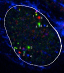
Figure 6: BAC probes of Chromosome 1 in a WI38 cell with homolog having 6 probes.

8 Proof for Theorem 3.2

Proof

Since it is sufficient to show that the theorem holds for the case of $k=2$, we assume in this proof that $k=2$ and each point-set $G_{i}$ has exactly two points. We make use of a construction by Dasgupta for the NP-hardness proof of the 2-mean clustering problem in high dimensional space [8]. Their proof reduces from the NAE3SAT problem. For better understanding our ideas, below we sketch their construction.

1. For any instance $\phi$ of NAE3SAT with literal set $\{x_{1},\cdots,x_{n}\}$ and $m$ clauses, construct a $2n\times 2n$ matrix $D_{\alpha,\beta}$ as follows, where the indices correspond to $\{x_{1},\cdots,x_{n}\}$ when they are in the range of $[1,n]$, and to $\{\overline{x_{1}},\cdots,\overline{x_{n}}\}$ when they are in the range of $[n+1,2n]$.
   $D_{\alpha,\beta}=\left\{\begin{array}[]{ll}0&\textrm{if $\alpha=\beta$}\\ 1+\Delta&\textrm{if $\alpha=\overline{\beta}$}\\ 1+\delta&\textrm{if $\alpha\sim\beta$}\\ 1&\textrm{otherwise,}\end{array}\right.$ where $\Delta$, $\delta$ are two constants satisfying inequalities $0<\delta<\Delta<1$ and $4\delta m<\Delta\leq 1-2\delta n$, and $\alpha\sim\beta$ means that both $\alpha$ and $\beta$ or both $\overline{\alpha}$ and $\overline{\beta}$ appear in a clause.

2. $D$ can be embedded into $R^{2n}$, i.e., there exist $2n$ points in $R^{2n}$ with $D$ as their distance matrix.

3. Let $C_{1}$ and $C_{2}$ be the two clusters of the $2$-mean clustering of the $2n$ embedding points. If for any $i$, the points corresponding to $x_{i}$ and $\overline{x_{i}}$ are separated into different clusters, then $\phi$ is satisfiable if and only if

   $$\frac{1}{2n}\sum_{i,j\in C_{1}}D_{i,j}+\frac{1}{2n}\sum_{i,j\in C_{2}}D_{i,j}\leq n-1+\frac{2\delta m}{n}.$$

4. Since $\frac{1}{2n}\sum_{i,j\in C_{1}}D_{i,j}+\frac{1}{2n}\sum_{i,j\in C_{2}}D_{i,j}$ is the total cost of the $2$-mean clustering for $C_{1}$ and $C_{2}$, a polynomial time solution to the $2$-mean clustering problem in high dimensional space implies a polynomial time solution to NAE3SAT. Thus the 2-mean clustering is NP-hard in high dimensions.

The above reduction can be naturally extended to show the NP-hardness of the full chromatic $2$-mean clustering problem. To show this, we only need to construct $G_{i}$ as the set containing the two points corresponding to $x_{i}$ and $\overline{x_{i}}$ (for simplicity, we write it as $G_{i}=\{x_{i},\overline{x_{i}}\}$), and the remaining proof follows from the same argument.

Next, we show that full $2$-CMean has no FPTAS in high dimensional space unless P=NP. To see this, we still use the same construction. From the above discussion, we know that $\phi$ is unsatisfiable if and only if for any chromatic partition of $\mathcal{G}$, there exists one clause in $\phi$ such that the three points corresponding to the three literals in this clause are clustered into the same cluster. Hence, the total cost for any chromatic partition is at least

$$2\frac{1}{n}({n\choose 2}+(m-1)\delta+3\delta)=n-1+\frac{2}{n}(m+2)\delta.$$

The ratio $\eta$ between the minimum chromatic partition cost of an unsatisfiable instance and the upper bound cost of a satisfiable instance is

$$\eta=\frac{n-1+\frac{2}{n}(m+2)\delta}{n-1+\frac{2\delta m}{n}}=1+\frac{\frac{4}{n}\delta}{n-1+\frac{2(m+2)}{n}\delta}.$$

If we let $\delta=\frac{1}{5m+2n}$, then $\eta=1+\frac{\frac{4}{n}\delta}{n-1+\frac{2(m+2)}{n}\delta}=1+\frac{4}{n(5m+2n)(n-1)+2(m+2)}$.

Suppose that there exists an FPTAS for the full chromatic $2$-means clustering problem. Then, if we let $\epsilon<\frac{4}{n(5m+2n)(n-1)+2(m+2)}$, the cost of a $(1+\epsilon)$-approximation of the full $2$-CMeans is less than $n-1+\frac{2}{n}(m+2)\delta$ if and only if $\phi$ is satisfiable. Since the running time of the FPTAS for full $2$-CMeans and $\frac{1}{\epsilon}$ are all polynomial functions of $m$ and $n$, this implies that NAE3SAT can be solved in polynomial time. Obviously this can only happen if P=NP. ∎

9 Proof of Lemma 3

Proof

In the our following discussion, we use $<a,b>$ to denote the inner product of $a$ and $b$. It is easy to see that

$$\sum_{p\in P}||p-m^{\prime}||^{2}=\sum_{p\in P}||p-m+m-m^{\prime}||^{2}$$

$$=\sum_{p\in P}(||p-m||^{2}+2<p-m,m-m^{\prime}>+||m-m^{\prime}||^{2})$$

$$=\sum_{p\in P}||p-m||^{2}+2\sum_{p\in P}<p-m,m-m^{\prime}>+|P|\times||m-m^{\prime}||^{2}$$

$$=\sum_{p\in P}||p-m||^{2}+2<\sum_{p\in P}(p-m),m-m^{\prime}>+|P|\times||m-m^{\prime}||^{2}.$$

Since $m$ is the mean point of $P$, $\sum_{p\in P}(p-m)=0$. Thus, the above equality becomes $\sum_{p\in P}||p-m^{\prime}||^{2}=\sum_{p\in P}||p-m||^{2}+|P|\times||m-m^{\prime}||^{2}$. ∎

10 Proof of Lemma 6

Proof

Similar to Lemma 5, we prove this lemma by mathematics induction on $j$.

Base case. For $j=1$, since $o_{1}=o$, we just need to let $\tau=o^{\prime}_{1}$. Then, we have $||\tau-o||=||o^{\prime}_{1}-o||=||o^{\prime}_{1}-o_{1}||\leq L\leq\sqrt{\epsilon}\delta+(1+\epsilon)L$. Thus, the base case holds.

Induction step. Assume that the lemma holds for any $j\leq j_{0}$ for some $j_{0}\geq 1$ (i.e., Induction Hypothesis). Now we consider the case of $j=j_{0}+1$. Similar to the proof of Lemma 5, we assume that $\frac{|P_{l}|}{|P|}\geq\frac{\epsilon}{4j}$ for each $1\leq l\leq j$. Otherwise, it can be reduced to a problem with smaller $j$, and solved by the induction hypothesis. Hence, in the following discussion, we assume that $\frac{|P_{l}|}{|P|}\geq\frac{\epsilon}{4j}$ for each $1\leq l\leq j$.

First, we know that $o=\sum^{j}_{l=1}\frac{|P_{l}|}{|P|}o_{l}$. Let $o^{\prime}=\sum^{j}_{l=1}\frac{|P_{l}|}{|P|}o^{\prime}_{l}$. Then, we have

$$||o-o^{\prime}||=||\sum^{j}_{l=1}\frac{|P_{l}|}{|P|}o_{l}-\sum^{j}_{l=1}\frac{|P_{l}|}{|P|}o^{\prime}_{l}||\leq\sum^{j}_{l=1}\frac{|P_{l}|}{|P|}||o_{l}-o^{\prime}_{l}||\leq L.$$ (10)

Thus, if we can find a grid point $\tau$ within a distance to $o^{\prime}$ no more than $\sqrt{\epsilon}\delta+\epsilon L$ (i.e., $||\tau-o^{\prime}||\leq\sqrt{\epsilon}\delta+\epsilon L$), by inequality (10), we will have $||\tau-o||\leq||\tau-o^{\prime}||+||o^{\prime}-o||\leq\sqrt{\epsilon}\delta+(1+\epsilon)L$. This means that we only need to find a grid point close enough to $o^{\prime}$.

To find such a $\tau$, we first consider the distance from $o^{\prime}_{l}$ to $o^{\prime}$. For any $1\leq l\leq j$, we have

$$||o^{\prime}_{l}-o^{\prime}||\leq||o^{\prime}_{l}-o_{l}||+||o_{l}-o||+||o-o^{\prime}||\leq 2\sqrt{\frac{j}{\epsilon}}\delta+2L,$$ (11)

where the first inequality follows from triangle inequality, and the second inequality follows from the facts that $||o^{\prime}_{l}-o_{l}||$ and $||o-o^{\prime}||$ are both bounded by $L$, and $||o_{l}-o||\leq 2\sqrt{\frac{j}{\epsilon}}\delta$ (by Lemma 4).

This implies that we can use the similar idea in Lemma 5 to construct a ball $\mathcal{B}$ centered at any $o^{\prime}_{l_{0}}$ and with radius $r=\max_{1\leq l\leq j}\{||o^{\prime}_{l}-o^{\prime}_{l_{0}}||\}$. Note that since $||o^{\prime}_{l}-o^{\prime}_{l_{0}}||\leq||o^{\prime}_{l}-o^{\prime}||+||o^{\prime}-o^{\prime}_{l_{0}}||\leq 4\sqrt{\frac{j}{\epsilon}}\delta+4L$ (by inequality (11)), the simplex $V^{\prime}$ is inside $\mathcal{B}$. Similar to Lemma 5, we can build a grid inside $\mathcal{B}$ with grid length $\frac{\epsilon r}{4j}$ and total grid points $O((8j/\epsilon)^{j})$. Clearly in this grid, we can find a grid point $\tau$ such that $||\tau-o^{\prime}||\leq\frac{\epsilon}{4\sqrt{j}}r\leq\sqrt{\epsilon}\delta+\epsilon L$. Thus, $||\tau-o||\leq\sqrt{\epsilon}\delta+(1+\epsilon)L$, and the induction step, as well as the lemma, holds. ∎

11 Proof of Claim 1 in Lemma 7

Proof

Since $1\geq\beta_{j}\geq\frac{1}{|\mathcal{G}|}\geq\frac{1}{kn}$, there is one integer $t$ between $1$ and $\log(kn)$, such that $2^{t-1}\leq\frac{1}{\beta_{j}}\leq 2^{t}$. Thus $2^{t/2-1}\sqrt{\epsilon}\delta_{opt}\leq\sqrt{\frac{\epsilon}{\beta_{j}}}\delta_{opt}\leq 2^{t/2}\sqrt{\epsilon}\delta_{opt}$. Together with $\delta\in[\delta_{opt},(1+\epsilon)\delta_{opt}]$, we have

$$2^{t/2-1}\sqrt{\epsilon}\frac{\delta}{1+\epsilon}\leq\sqrt{\frac{\epsilon}{\beta_{j}}}\delta_{opt}\leq 2^{t/2}\sqrt{\epsilon}\delta.$$

Thus if set $\hat{r}_{j}=2^{t/2}\sqrt{\epsilon}\delta$, we have $\sqrt{\frac{\epsilon}{\beta_{j}}}\delta_{opt}\leq\hat{r}_{j}\leq 2(1+\epsilon)\sqrt{\frac{\epsilon}{\beta_{j}}}\delta_{opt}$. Let $x=\frac{j\hat{r}_{j}}{j\sqrt{\frac{\epsilon}{\beta_{j}}}\delta_{opt}}$. Then we have $1\leq x\leq 2(1+\epsilon)$. We build a grid in the interval $[\frac{x}{2(1+\epsilon)},x]$ with the grid length $\frac{\epsilon}{4(1+\epsilon)}x$, and obtain a grid set (i.e., number set) $\mathcal{N}=\{\frac{1+l\frac{\epsilon}{2}}{2(1+\epsilon)}x\mid 0\leq l\leq 4+\frac{2}{\epsilon}\}$. We prove that there must exist one number in $\mathcal{N}$ and is between $1$ and $1+\epsilon/2$. First, we know that $\frac{x}{2(1+\epsilon)}\leq 1\leq x$. If $x\leq 1+\epsilon/2$, we find the the desired number $x$ in $\mathcal{N}$. Otherwise, the whole interval $[1,1+\epsilon/2]$ is inside $[\frac{x}{2(1+\epsilon)},x]$. Since the grid has grid length $\frac{\epsilon}{4(1+\epsilon)}x\leq\frac{\epsilon}{4(1+\epsilon)}2(1+\epsilon)=\epsilon/2$, there must exist one grid point locating inside $[1,1+\epsilon/2]$. Thus, the desired number exists in $\mathcal{N}$.

Let $\mathcal{R}_{j}=\{\frac{1+l\frac{\epsilon}{2}}{2(1+\epsilon)}j\hat{r}_{j}\mid 0\leq l\leq 4+\frac{2}{\epsilon}\}$. From the above analysis, we know that there exists one value $r_{j}\in\mathcal{R}_{j}$ such that

$$j\sqrt{\frac{\epsilon}{\beta_{j}}}\delta_{opt}\leq r_{j}\leq(1+\frac{\epsilon}{2})j\sqrt{\frac{\epsilon}{\beta_{j}}}\delta_{opt}.$$

Note that $\mathcal{R}_{j}\subset\mathcal{R}$, where $\mathcal{R}=\cup^{\log(kn)}_{t=0}\{\frac{1+l\frac{\epsilon}{2}}{2(1+\epsilon)}j2^{t/2}\sqrt{\epsilon}\delta\mid 0\leq l\leq 4+\frac{2}{\epsilon}\}$. Thus, the Claim is proved.

∎

12 Proof of Claim 2 in Lemma 7

Proof

First, for each $1\leq l\leq j-1$, we have $|Opt_{l}\setminus(\bigcup^{j-1}_{w=1}B_{j,w})|\leq|Opt_{l}\setminus B_{j,l}|$. Secondly, by Markov inequality, we have

$$|Opt_{l}\setminus B_{j,l}|\leq\frac{\delta^{2}_{l}}{(r_{j}-||p_{v_{l}}-m_{l}||)^{2}}|Opt_{l}|.$$

Note that $\delta^{2}_{opt}=\sum^{k}_{j=1}\beta_{j}\delta^{2}_{j}$, and $\beta_{j}\leq\beta_{l}$ (by $l<j$). Thus, we have $\delta_{l}\leq\sqrt{\frac{1}{\beta_{l}}}\delta_{opt}\leq\sqrt{\frac{1}{\beta_{j}}}\delta_{opt}$. Together with $j\sqrt{\frac{\epsilon}{\beta_{j}}}\delta_{opt}\leq r_{j}$ and $||p_{v_{l}}-m_{l}||\leq\epsilon\delta_{l}+(1+\epsilon)l\sqrt{\frac{\epsilon}{\beta_{l}}}\delta_{opt}$ (by induction hypothesis), we have

$$r_{j}-||p_{v_{l}}-m_{l}|| \geq j\sqrt{\frac{\epsilon}{\beta_{j}}}\delta_{opt}-(\epsilon\delta_{l}+(1+\epsilon)(j-1)\sqrt{\frac{\epsilon}{\beta_{l}}}\delta_{opt})$$

$$= (1-(j-1)\epsilon)\sqrt{\frac{\epsilon}{\beta_{j}}}\delta_{opt}-\epsilon\delta_{l}$$

$$\geq (1-(j-1)\epsilon-\sqrt{\epsilon})\sqrt{\frac{\epsilon}{\beta_{j}}}\delta_{opt},$$

where the last inequality follows from $\delta_{l}\leq\sqrt{\frac{1}{\beta_{l}}}\delta_{opt}\leq\sqrt{\frac{1}{\beta_{j}}}\delta_{opt}$. Thus, we have

$$|Opt_{l}\setminus B_{j,l}| \leq \frac{\delta^{2}_{l}}{(1-(j-1)\epsilon-\sqrt{\epsilon})^{2}\frac{\epsilon}{\beta_{j}}\delta^{2}_{opt}}|Opt_{l}|$$

$$\leq \frac{\delta^{2}_{l}}{(1-(j-1)\epsilon-\sqrt{\epsilon})^{2}\frac{\epsilon}{\beta_{j}}\beta_{l}\delta^{2}_{l}}|Opt_{l}|$$

$$= \frac{\beta_{j}}{(1-(j-1)\epsilon-\sqrt{\epsilon})^{2}\epsilon\beta_{l}}|Opt_{l}|$$

$$= \frac{\beta_{j}|\mathcal{G}|}{(1-(j-1)\epsilon-\sqrt{\epsilon})^{2}\epsilon}\leq\frac{\beta_{j}|\mathcal{G}|}{(1-j\sqrt{\epsilon})^{2}\epsilon},$$

where the second inequality follows from the fact that $\beta_{l}\delta^{2}_{l}\leq\delta^{2}_{opt}$, and the fourth equation follows from that $\frac{|Opt_{l}|}{\beta_{l}}=|\mathcal{G}|$. Note that we can assume $\epsilon$ is small enough such that $\epsilon\leq\frac{1}{4j^{2}}$, which implies that $\frac{\beta_{j}|\mathcal{G}|}{(1-j\sqrt{\epsilon})^{2}\epsilon}\leq\frac{4\beta_{j}|\mathcal{G}|}{\epsilon}$. Otherwise, we can just replace $\epsilon$ by $\frac{\epsilon}{4j^{2}}$ as the input at the beginning of the algorithm. Thus, in total, we have

$$|Opt_{l}\setminus B_{j,l}| \leq \frac{4\beta_{j}|\mathcal{G}|}{\epsilon}.$$

Thus the Claim is proved. ∎

13 Proof of Claim 3 in Lemma 7

Proof

First, we have

$$\frac{|P_{1}|}{|P_{1}\cup P_{j}|}\geq\frac{\frac{1}{j-1}(1-\frac{\epsilon^{3}}{j})}{\frac{1}{j-1}(1-\frac{\epsilon^{3}}{j})+\frac{\epsilon^{3}}{j}}>\frac{1-\epsilon^{3}}{1+\epsilon^{3}}.$$

Let $a^{2}$ denote the variance of $P_{1}\cup P_{j}$. By Lemma 4, we know that $||\tau_{1}-\tau^{\prime}||\leq\sqrt{\frac{2\epsilon^{3}}{1-\epsilon^{3}}}a$. Meanwhile, since $\frac{|P_{1}\cup P_{j}|}{|Opt_{j}|}\geq\frac{|P_{1}|}{|Opt_{j}|}\geq\frac{\frac{1}{j-1}(\beta_{j}-\epsilon^{3}\frac{\beta_{j}}{j})|\mathcal{G}|}{\beta_{j}|\mathcal{G}|}=\frac{1-\frac{\epsilon^{3}}{j}}{j-1}$, we have $a^{2}\leq\frac{|Opt_{j}|}{|P_{1}\cup P_{j}|}\delta^{2}_{j}\leq\frac{j-1}{1-\frac{\epsilon^{3}}{j}}\delta^{2}_{j}$. Then we have

$$||\tau_{1}-\tau^{\prime}|| \leq \sqrt{\frac{2\epsilon^{3}}{1-\epsilon^{3}}}a\leq\sqrt{\frac{2\epsilon^{3}}{1-\epsilon^{3}}}\sqrt{\frac{j-1}{1-\frac{\epsilon^{3}}{j}}}\delta_{j}$$

$$\leq \sqrt{\frac{2j\epsilon^{3}}{(1-\epsilon^{3})(1-\frac{\epsilon^{3}}{j})\beta_{j}}}\delta_{opt}$$

$$\leq \sqrt{\frac{2j\epsilon^{3}}{(1-\epsilon^{3})(1-\epsilon^{3})\beta_{j}}}\delta_{opt}=\frac{\sqrt{2}\epsilon}{1-\epsilon^{3}}\sqrt{\frac{j\epsilon}{\beta_{j}}}\delta_{opt},$$

where the third inequality follows from $\delta_{j}\leq\sqrt{\frac{1}{\beta_{j}}}\delta_{opt}$. Thus, the claim is true. ∎

14 Chromatic $k$-Medians Clustering

In this section, we extend our ideas for $k$-CMeans to the Chromatic $k$-Medians Clustering problem ($k$-CMedians). Similar to $k$-CMeans, we first show its relationship with $k$-medians (in Section 14.1), and then present a $(5+\epsilon)$-approximation algorithm (in Section 14.2). Due to the lack of a similar Simplex Lemma for $k$-CMedians, we achieve a constant approximation, instead of a PTAS.

Definition 3 (Chromatic $k$-Median Clustering ($k$-CMedians))

Let $\mathcal{G}=\{G_{1},\cdots,$ $G_{n}\}$ be a set of $n$ point-sets with each $G_{i}=\{p^{i}_{1},\dots,p^{i}_{k_{i}}\}$ consisting of $k_{i}\leq k$ points in $\mathbb{R}^{d}$ space. The chromatic $k$-median clustering (or $k$-CMedians) of $\mathcal{G}$ is to find $k$ points $\{m_{1},\cdots,m_{k}\}$ in $\mathbb{R}^{d}$ space and a chromatic partition $U_{1},\cdots,U_{k}$ of $\mathcal{G}$ such that $\frac{1}{n}\sum_{j}\sum_{q\in U_{j}}||q-m_{j}||$ is minimized.

14.1 Constant Approximation from $k$-Medians

Given a set of points in $\mathbb{R}^{d}$, the optimal median point is also called Fermat Weber point in geometry. Its main difference with mean point is that no explicit formula exists for computing the optimal median point, while the mean point is simply the average of the given points. Consequently, median point is often approximated using some iterative procedure, such as Weiszfeld’s algorithm. Thus in the following discussion, we only assume the availability of a $(1+\epsilon)$-approximation of the median point.

Lemma 9

Let $P$ be a set of points in $\mathbb{R}^{d}$ space, and $P_{1}$ be a subset of $P$ containing a fraction of $\alpha\leq 1$ points of $P$. Let $m_{opt}$ and $m$ be the optimal and $(1+\epsilon)$-approximate median point of $P$ respectively, and $m_{1}$ be the optimal median of $P_{1}$. Then $||m_{1}-m||\leq\frac{2+\epsilon}{\alpha}\mu$, where $\mu=\frac{1}{|P|}\sum_{p\in P}||p-m_{opt}||$.

Proof

Let $\mu_{1}=\frac{1}{|P_{1}|}\sum_{p\in P_{1}}||p-m_{1}||$. Since $P_{1}\subseteq P$, it is easy to know that $\sum_{p\in P}||p-m||\geq\sum_{p\in P_{1}}||p-m||$, which implies that $(1+\epsilon)\mu\geq\frac{1}{|P|}\sum_{p\in P_{1}}||p-m||=\alpha\frac{1}{|P_{1}|}\sum_{p\in P_{1}}||p-m||$. By triangle inequality, we also have $||p-m||\geq||m-m_{1}||-||p-m_{1}||$. Thus,

$$(1+\epsilon)\mu\geq\alpha(||m-m_{1}||-\mu_{1}).$$ (12)

Since $m_{1}$ is the optimal median of $P_{1}$, we have $\mu_{1}=\frac{1}{|P_{1}|}\sum_{p\in P_{1}}||p-m_{1}||\leq\frac{1}{|P_{1}|}\sum_{p\in P_{1}}||p-m_{opt}||\leq\frac{1}{|P_{1}|}\sum_{p\in P}||p-m_{opt}||=\frac{1}{\alpha}\mu$. Plugging this into inequality (12), we have $||m-m_{1}||\leq\frac{2+\epsilon}{\alpha}\mu$. ∎

Theorem 14.1

Let $\mathcal{G}=\{G_{1},\cdots,G_{n}\}$ be an instance of $k$-CMedians, and $\mathcal{C}$ be the $k$ $(1+\epsilon)$-approximate median points of the $k$ clusters generated by a $c$-approximation $k$-medians algorithm on the points $\cup_{i=1}^{n}G_{i}$. Then, $[\mathcal{C}]^{k}$ contains at least one $k$-tuple whose elements are the $k$ median points of a $((2+\epsilon)ck^{2}+(2+\epsilon)k+1)$-approximation of $k$-CMedians on $\mathcal{G}$, where $[\mathcal{C}]^{k}=\underbrace{\mathcal{C}\times\cdots\times\mathcal{C}}_{k}$.

Proof

Let $\{c_{1},\cdots,c_{k}\}$ be the set of $k$ approximate median points in $\mathcal{C}$, and $\{S_{1},\cdots,S_{k}\}$ be the $k$ clusters returned by the $c$-approximation $k$-medians algorithm. Thus, $c_{j}$ is the $(1+\epsilon)$-approximate median point of $S_{j}$ for $1\leq j\leq k$. Let $\mathcal{OPT}=\{Opt_{1},\cdots,Opt_{k}\}$ be the unknown optimal solution for $k$-CMedians on $\mathcal{G}$, and $m_{j}$ be the optimal median point of $Opt_{j}$ for $1\leq j\leq k$. Denote the set $Opt_{i}\cap S_{j}$ as $\Gamma^{i}_{j}$, and its optimal median point as $\tau^{i}_{j}$ for $1\leq i,j\leq k$ .

Since $\cup^{k}_{j=1}\Gamma^{i}_{j}=Opt_{i}$, there must exist some index $1\leq j_{i}\leq k$ such that $|\Gamma^{i}_{j_{i}}|\geq\frac{1}{k}|Opt_{i}|$. Fixing $j_{i}$, we have the following about $\sum_{p\in Opt_{i}}||p-c_{j_{i}}||$.

$$\sum_{p\in Opt_{i}}||p-c_{j_{i}}|| = \sum_{p\in Opt_{i}}||p-m_{i}+m_{i}-c_{j_{i}}||$$

$$\leq \sum_{p\in Opt_{i}}(||p-m_{i}||+||m_{i}-c_{j_{i}}||)$$

$$= \sum_{p\in Opt_{i}}||p-m_{i}||+|Opt_{i}|\times||m_{i}-c_{j_{i}}||$$

$$= \sum_{p\in Opt_{i}}||p-m_{i}||+|Opt_{i}|\times||m_{i}-\tau^{i}_{j_{i}}+\tau^{i}_{j_{i}}-c_{j_{i}}||$$

$$\leq \sum_{p\in Opt_{i}}||p-m_{i}||+|Opt_{i}|\times(||m_{i}-\tau^{i}_{j_{i}}||+||\tau^{i}_{j_{i}}-c_{j_{i}}||)$$

By Lemma 9, we have

$$||\tau^{i}_{j_{i}}-m_{i}|| \leq \frac{2+\epsilon}{\frac{1}{k}}(\frac{1}{|Opt_{i}|}\sum_{p\in Opt_{i}}||p-m_{i}||);$$

$$||\tau^{i}_{j_{i}}-c_{j_{i}}|| \leq \frac{2+\epsilon}{\frac{|\Gamma^{i}_{j_{i}}|}{|S_{j_{i}}|}}(\frac{1}{|S_{j_{i}}|}\sum_{p\in S_{j_{i}}}||p-c_{j_{i}}||).$$

From the above inequalities, we have

$$\sum_{p\in Opt_{i}}||p-c_{j_{i}}|| \leq \sum_{p\in Opt_{i}}||p-m_{i}||+|Opt_{i}|\times(||m_{i}-\tau^{i}_{j_{i}}||+||\tau^{i}_{j_{i}}-c_{j_{i}}||)$$

$$\leq \sum_{p\in Opt_{i}}||p-m_{i}||^{2}+|Opt_{i}|(\frac{2+\epsilon}{\frac{1}{k}}(\frac{1}{|Opt_{i}|}\sum_{p\in Opt_{i}}||p-m_{i}||)+\frac{2+\epsilon}{\frac{|\Gamma^{i}_{j_{i}}|}{|S_{j_{i}}|}}(\frac{1}{|S_{j_{i}}|}\sum_{p\in S_{j_{i}}}||p-c_{j_{i}}||))$$

$$= ((2+\epsilon)k+1)\sum_{p\in Opt_{i}}||p-m_{i}||+(2+\epsilon)\frac{|Opt_{i}|}{|\Gamma^{i}_{j_{i}}|}\times\sum_{p\in S_{j_{i}}}||p-c_{j_{i}}||).$$

Since $|\Gamma^{i}_{j_{i}}|\geq\frac{1}{k}|Opt_{i}|$, we have $\frac{|Opt_{i}|}{|\Gamma^{i}_{j_{i}}|}\leq k$. Thus,

$$\sum_{p\in Opt_{i}}||p-c_{j_{i}}||^{2}\leq((2+\epsilon)k+1)\sum_{p\in Opt_{i}}||p-m_{i}||+(2+\epsilon)k\sum_{p\in S_{j_{i}}}||p-c_{j_{i}}||.$$

Summing both sides of the above inequality over $i$, we have

$$\sum^{k}_{i=1}\sum_{p\in Opt_{i}}||p-c_{j_{i}}||^{2} \leq ((2+\epsilon)k+1)\sum^{k}_{i=1}\sum_{p\in Opt_{i}}||p-m_{i}||+(2+\epsilon)k\sum^{k}_{i=1}\sum_{p\in S_{j_{i}}}||p-c_{j_{i}}||$$ (13)

$$\leq ((2+\epsilon)k+1)\sum^{k}_{i=1}\sum_{p\in Opt_{i}}||p-m_{i}||+(2+\epsilon)k^{2}\sum^{k}_{j=1}\sum_{p\in S_{j}}||p-c_{j}||.$$

It is easy to know that the optimal objective value of $k$-medians is no larger than that of $k$-CMedians on the same set of points in $\mathcal{G}$. Thus, $\sum^{k}_{j=1}\sum_{p\in S_{j}}||p-c_{j}||\leq c\sum^{k}_{i=1}\sum_{p\in Opt_{i}}||p-m_{i}||$. Plugging this inequality into (13), we have

$$\sum^{k}_{i=1}\sum_{p\in Opt_{i}}||p-c_{j_{i}}||\leq((2+\epsilon)ck^{2}+(2+\epsilon)k+1)\sum^{k}_{i=1}\sum_{p\in Opt_{i}}||p-m_{i}||.$$

The above inequality means that if we take the $k$-tuple $(c_{j_{1}},\cdots,c_{j_{k}})$ as the $k$ approximate median points for $k$-CMedians, we have a $((2+\epsilon)ck^{2}+(2+\epsilon)k+1)$-approximation solution for $k$-CMedians. Thus, the theorem is proved. ∎

14.2 Peeling Algorithm for $k$-CMedians

The following lemma is a key to the peeling algorithm for $k$-CMedians (i.e., play a similar role as Lemma 5 for $k$-CMeans).

Lemma 10

Let $P$ to be a set of points in $\mathbb{R}^{d}$ with a partition $P=\cup^{j}_{l-1}P_{l}$, $o$ be its optimal median point, and $o_{l}$ be the optimal median point of $P_{l}$ for $1\leq l\leq j$. Let $\mu=\frac{1}{|P|}\sum_{p\in P}||p-o||$. Then, there exists some $i_{0}$ such that $||o-o_{i_{0}}||\leq 4\mu$.

Proof

Since $\mu=\frac{\sum_{p\in P}||p-o||}{|P|}=\sum^{l}_{i=1}(\frac{|P_{i}|}{|P|}\frac{\sum_{p\in P_{i}}||p-o||}{|P_{i}|})$, there must exist some index $i_{0}$ such that $\frac{\sum_{p\in P_{i_{0}}}||p-o||}{|P_{i_{0}}|}$ $\leq\mu$. By Markov inequality, we know that there exists one subset $U$ of $P_{i_{0}}$ such that $|U|>|P_{i_{0}}|/2$ and $||p-o||\leq 2\mu$ for any $p\in U$.

Since $o_{i_{0}}$ is the optimal median point of $P_{i_{0}}$, $\frac{\sum_{p\in P_{i_{0}}}||p-o_{i_{0}}||}{|P_{i_{0}}|}\leq\frac{\sum_{p\in P_{i_{0}}}||p-o||}{|P_{i_{0}}|}\leq\mu$. Similarly, by Markov inequality, we know that there exists one subset $V$ of $P_{i_{0}}$ such that $|V|>|P_{i_{0}}|/2$ and $||p-o_{i_{0}}||\leq 2\mu$ for any $p\in V$.

From the inequalities of $|U|>|P_{i_{0}}|/2$ and $|V|>|P_{i_{0}}|/2$ and the fact that $U\cap V\neq\emptyset$, we know that there exists one point $p_{0}\in U\cap V$ such that $||p_{0}-o||\leq 2\mu$ and $||p_{0}-o_{i_{0}}||\leq 2\mu$. Thus $||o_{i_{0}}-o||\leq||o_{i_{0}}-p_{0}||+||p_{0}-o||\leq 4\mu$. ∎

Before presenting our peeling algorithm, we still need the following lemma proved by Badoiu et al. in [6] for finding an approximate solution for $1$-median.

Theorem 14.2 ([6])

Let $P$ be a normalized set of $n$ points in $\mathbb{R}^{d}$ space, $1>\epsilon>0$, and $R$ be a random sample of $O(1/\epsilon^{3}\log 1/\epsilon)$ points from $P$. Then one can compute, in $O(d2^{O(1/\epsilon^{4})}\log n)$ time, a point-set $S(P,R)$ of cardinality $O(2^{O(1/\epsilon^{4})}\log n)$ , such that with constant probability (over the choices of $R$), there is a point $q\in S(P,R)$ such that $cost(q,P)\leq(1+\epsilon)med_{opt}(P,1)$.

Algorithm $k$-CMedians
Input: $\mathcal{G}=\{G_{1},\cdots,G_{n}\}$, $k\geq 2$ and an small constant $\epsilon>0$.
Output: a $(5+\epsilon)$-approximation solution for $k$-CMedians on $\mathcal{G}$.

1. Run the $(1+\epsilon)$-approximation $k$-medians algorithm from [15] on $\mathcal{G}$, and let $\Omega$ be the obtained objective value.

2. For $i=1$ to $\frac{4k}{\epsilon}$ do

   1. Set $\delta=\frac{\Omega}{4k}+i\frac{\epsilon}{4k}\Omega$, and run Algorithm Sphere-Peeling-Tree-2.

   2. Let $\mathcal{T}_{i}$ be the returned tree.

3. For each path of every $\mathcal{T}_{i}$, use bipartite matching procedure to compute the objective value of $k$-CMeans on $\mathcal{G}$. Output the $k$ points from the path with smallest objective value.

Algorithm Sphere-Peeling-Tree-$2$
Input: $\mathcal{G}$, $k\geq 2$, $\epsilon,\delta>0$.
Output: A tree $\mathcal{T}$ of height $k$ with each node $v$ associated with a point $p_{v}\in\mathbb{R}^{d}$.

1. Initialize $\mathcal{T}$ with a single root node $v$ associating with no point.

2. Recursively grow each node $v$ in the following way

   1. If the height of $v$ is already $k$, then it is a leaf node.

   2. Otherwise, let $j$ be the height of $v$. Build the set of radius candidates $\mathcal{R}=\cup^{\log(kn)}_{t=0}\{\frac{1+l\frac{\epsilon}{2}}{2(1+\epsilon)}j2^{t/2}\sqrt{\epsilon}\delta\mid 0\leq l\leq 4+\frac{2}{\epsilon}\}$.For each radius candidate $r\in\mathcal{R}$ do

      1. Let $j$ be the height of $v$, and $\{p_{v_{1}},\cdots,p_{v_{j}}\}$ be the $j$ points associated with nodes on the root-to-$v$ path (including $p_{v}$).

      2. For each $p_{v_{l}}$, $1\leq l\leq j$, construct a ball $B_{j,l}$ centered at $p_{v_{l}}$ and with radius $r$.

      3. Take a random sample from $\mathcal{G}\setminus\cup^{j}_{l=1}B_{j,l}$ with size $m=\frac{8k^{3}}{\epsilon^{9}}\ln\frac{k^{2}}{\epsilon^{6}}$. Compute the approximate median points of all subsets of the sample (by Theorem 14.2), and denote the set of the approximate median points as $\Pi$. Clearly, $|\Pi|=2^{m+O(1/\epsilon^{4})}\log n$.

      4. For each point $p$ in $\Pi$, add one child to $v$, and associate it with $p$; add another $j$ children, with each one associating with a different point in $\{p_{v_{1}},\cdots,p_{v_{j}}\}$.

We can use a similar approach as in Section 5.3 to analyze the correctness of Algorithm $k$-CMedians.

Let $\mathcal{OPT}=\{Opt_{1},\cdots,Opt_{k}\}$ be the optimal solution of $k$-CMedians on $\mathcal{G}$. Without loss of generality, we assume that $|Opt_{1}|\geq|Opt_{2}|\geq\cdots\geq|Opt_{k}|$. For each $Opt_{j}$, $1\leq j\leq k$, let $m_{j}$ be its median point, $\beta_{j}$ be its fraction in $\mathcal{G}$ (i.e., $|Opt_{j}|/|\cup_{i=1}^{n}G_{i}|$), and $\mu_{j}=\frac{1}{|Opt_{j}|}\sum_{p\in Opt_{j}}||p-m_{j}||$. Thus, $\beta_{1}\geq\cdots\geq\beta_{k}$ and $\sum^{k}_{j=1}\beta_{j}=1$. Also, let $\mu_{opt}=\sum^{k}_{j=1}\beta_{j}\mu_{j}$.

Lemma 11

Among all the trees generated in Algorithm $k$-CMedians, there exists one tree $\mathcal{T}_{i}$, which has a root-to-leaf path with each node $v_{j}$ at level $j$, $1\leq j\leq k$, on the path associating a point $p_{v_{j}}$ and satisfying the inequality

$$||p_{v_{j}}-m_{j}||\leq 4\mu_{j}+(1+\epsilon)j\frac{\epsilon}{\beta_{j}}\mu_{opt}.$$

Lemma 12

If Lemma 11 is true, Algorithm $k$-CMedians yields a $(5+O(k^{2})\epsilon)$-approximation solution for $k$-CMedians.

Proof

We first assume that Lemma 11 is true. Then for each $1\leq j\leq k$, we have

$$\sum_{p\in Opt_{j}}||p-p_{v_{j}}|| \leq \sum_{p\in Opt_{j}}||p-m_{j}||+|Opt_{j}|\times||m_{j}-p_{v_{j}}||$$ (14)

$$\leq \sum_{p\in Opt_{j}}||p-m_{j}||+|Opt_{j}|\times(4\mu_{j}+(1+\epsilon)j\frac{\epsilon}{\beta_{j}}\mu_{opt})$$

$$= 5|Opt_{j}|\mu_{j}+(1+\epsilon)j\epsilon|\mathcal{G}|\mu_{opt}$$

Summing the both sides of (14) over $j$, we have

$$\sum^{k}_{j=1}\sum_{p\in Opt_{j}}||p-p_{v_{j}}||^{2} \leq \sum^{k}_{j=1}(5|Opt_{j}|\mu_{j}+(1+\epsilon)j\epsilon|\mathcal{G}|\mu_{opt})$$ (15)

$$\leq 5\sum^{k}_{j=1}|Opt_{j}|\mu_{j}+(1+\epsilon)k^{2}\epsilon|\mathcal{G}|\mu_{opt}$$

$$= (5+O(k^{2})\epsilon)|\mathcal{G}|\mu_{opt}.$$

In the above, the last equation follows from the fact that $\sum^{k}_{j=1}|Opt_{j}|\mu_{j}=|\mathcal{G}|\mu_{opt}$. By (15), we know that $\{p_{v_{1}},\cdots,p_{v_{k}}\}$ induces a $(5+O(k^{2})\epsilon)$-approximation solution for $k$-CMedians. ∎

By a similar argument given in the proof of Lemma 7, we can show the correctness of Lemma 11. Thus, we have the following theorem.

Theorem 14.3

With constant probability, Algorithm $k$-CMedians yields a $(5+\epsilon)$-approximation for $k$-CMedians in $O(2^{poly(\frac{k}{\epsilon})}n(\log n)^{2k}d)$ time.

References

- [1] Esther M. Arkin, Jos Miguel D az-B ez, Ferran Hurtado, Piyush Kumar, Joseph S. B. Mitchell, Bel n Palop, Pablo P rez-Lantero, Maria Saumell, Rodrigo I. Silveira: Bichromatic 2-Center of Pairs of Points. LATIN 2012: 25-36
- [2] P. K. Agarwal and C. M. Procopiuc. “Exact and Approximation Algorithms for Clustering,”Proc. 9th ACM-SIAM Sympos. Discrete Algorithms, pages 658-667, 1998.
- [3] David Arthur, Sergei Vassilvitskii: ”k-means++: the advantages of careful seeding”. SODA 2007: 1027-1035
- [4] Nikhil Bansal, Avrim Blum, Shuchi Chawla: ”Correlation Clustering”.Machine Learning 56(1-3): 89-113 (2004)
- [5] S.Basu, Ian Davidson: Clustering with Constraints Theory and Practice. ACM KDD 2006
- [6] M.Badoiu, S.Har-Peled, P.Indyk, “Approximate clustering via core-sets”, Proceedings of the 34th Symposium on Theory of Computing, pp. 250–257, 2002.
- [7] C.Böhm, K.Kailing, P.Kröger, A.Zimek, ”Computing Clusters of Correlation Connected Objects”.Proc. ACM SIGMOD International Conference on Management of Data (SIGMOD’04), Paris, France. pp. 455–467. doi:10.1145/1007568.1007620.
- [8] S. Dasgupta, ”The hardness of k-means clustering”. Technical Report, 2008.
- [9] Erik Demaine, Dotan Emanuel, Amos Fiat, and Nicole Immorlica. ”Correlation clustering in general weighted graphs”. Theor. Comput. Sci., 361(2):172-187, 2006
- [10] H.Ding, J.Xu, ”Solving Chromatic Cone Clustering via Minimum Spanning Sphere”, ICALP, 2011
- [11] Ioannis Giotis and Venkatesan Guruswami. ” Correlation clustering with a fixed number of clusters”. Theory of Computing, 2(1):249-266, 2006.
- [12] S. Har-Peled and S. Mazumdar, “Coresets for k-Means and k-Median Clustering and their Applications,” Proc. 36th ACM Symposium on Theory of Computing, pages 291-300, 2004.
- [13] Mary Inaba, Naoki Katoh, Hiroshi Imai, ” Applications of Weighted Voronoi Diagrams and Randomization to Variance-Based k-Clustering (Extended Abstract)”. Symposium on Computational Geometry 1994: 332-339
- [14] S. G. Kolliopoulos and S. Rao, “A nearly linear-time approximation scheme for the euclidean k-median problem,” Proc. 7th Annu. European Sympos. Algorithms, pages 378-389, 1999.
- [15] A. Kumar, Y. Sabharwal, S. Sen, ” Linear-time approximation schemes for clustering problems in any dimensions”. J. ACM 57(2):2010
- [16] R.Ostrovsky, Y.Rabani, L.J.Schulman, and C.Swamy. ”The Effectiveness of Lloyd-Type Methods for the k-Means Problem”. Proceedings of the 47th Annual IEEE Symposium on Foundations of Computer Science (FOCS’06). pp. 165–174.