Abstract

Weak amplification is a signal enhancement technique which is used to measure tiny changes that otherwise cannot be determined because of technical limitations. It is based on the existence of a special type of interaction which couples a property of a system, i.e., polarization or which-path information, with a separate degree of freedom, i.e., transverse position or frequency. Unfortunately, the weak amplification process is generally accompanied by severe losses of the detected signal, which limits the applicability of the weak amplification concept. However, we will show here that since the weak measurement concept is essentially an interference phenomena, it should be possible to use the degree of interference to get relevant information about the physical system under study in a more general scenario, where the signal is not severely depleted (high-signal regime). This can widen the range of systems where the weak measurement concept can be applied. In this scenario, which can be called generally weak interference, the idea of weak value does not convey any useful information.

OCIS codes: (030.1670) Coherent optical effects; (270.0270) Quantum optics; (350.7420) Other areas of optics: Waves

juanp.torres@icfo.es

1 Introduction

A weak measurement is a concept first introduced by Aharonov, Albert, and Vaidman [1], which describes a situation where two subsystems interact, even though through a weakly coupling process. Generally, the weak measurement idea is presented in the general framework of Quantum Mechanics, where one of the subsystems is assumed to be the measuring device, whose aim is to unveil the value of a property that characterizes the other interacting subsystem (the system).

The fact that the coupling is weak can be seemingly disadvantageous, since it is expected to produce an uncertainty in the measurement larger than the values that should be differentiated. However, when appropriate initial and final states of the system to be measured are selected, for instance by choosing them to be nearly orthogonal, the mean value of the reading of the measuring system can yield an unexpectedly large value (weak amplification). Surprisingly, this value can lay outside the range of small displacements of the measurement pointer caused by each one of the possible states of the system. Unfortunately, this is also accompanied by a severe depletion of the intensity of the signal detected, due to the quasi-orthogonality of the input and final states of the system. This prevents the applicability of the weak measurement concept to experiments which are already limited by a low signal-to-noise ratio [2], since the intensity of the detected signal is severely decreased.

For instance, when considering the refraction of a light beam in a thin birefringent crystal, the two orthogonal linear polarizations components of the optical beam are displaced a small distance $\Delta$ compared with the beam waist [3]. For a given initial $|\Psi_{in}\rangle$ and final $|\Psi_{out}\rangle$ states of the polarization of the system, so that $\langle\Psi_{out}|\Psi_{in}\rangle\sim\epsilon$ ($\epsilon$ is small), the mean value of the shift of the position of the light beam is $\langle x\rangle/\Delta=\Re\left(\langle A\rangle_{w}\right)$, where the weak value $\langle A\rangle_{w}$ is defined as

$$\langle A\rangle_{w}=\frac{\langle\Psi_{out}|A|\Psi_{in}\rangle}{\langle\Psi_{out}|\Psi_{in}\rangle}\sim\frac{1}{\epsilon}.$$ (1)

In this example, the power of the output signal ($P_{out}$) is severely reduced, i.e., $P_{out}/P_{in}\sim\epsilon^{2}/2$. The signal enhancement of the position of the beam due to weak amplification can thus be observed only if the input signal intensity ($P_{in}$) can be enhanced.

Most experimental realizations of weak measurements up to date take place in this context. This is the case for experiments that use the polarization of a light beam to reveal extremely small spatial displacements [2, 3], and for experiments that make use of the two counter-propagating paths in a Sagnac interferometer to detect tiny beam deflections [4], or tiny frequency shifts [5]. Interestingly, weak measurements can have a wider range of applicability than originally conceived, appearing naturally in the context of optical telecom networks [6], and the description of the response function of a system [7].

Even though the idea of weak measurement was born in the context of Quantum Mechanics, and is generally formulated in the language of Quantum Mechanics, it can be understood as the consequence of the constructive and destructive interference between the complex amplitudes of different pointer states [8]. Each of these correspond to the nearly equal readings of the measuring device for each value of the state of the system. The concept behind a weak measurement, also termed as weak amplification, can thus be applied to any physical wave phenomena and explained in classical terms as a wave interference process [9].

Here we will show that since a weak measurement is an interference phenomenon, its effect should be noticeable even in the regime of small losses, where the concept of weak value might not convey any relevant information about the system or the measuring device. This can open new applications based on weak interference, especially for interactions where it is not possible to enhance the signal-to-noise ratio of the measurement. For example, when the intensity of the input signal cannot be increased.

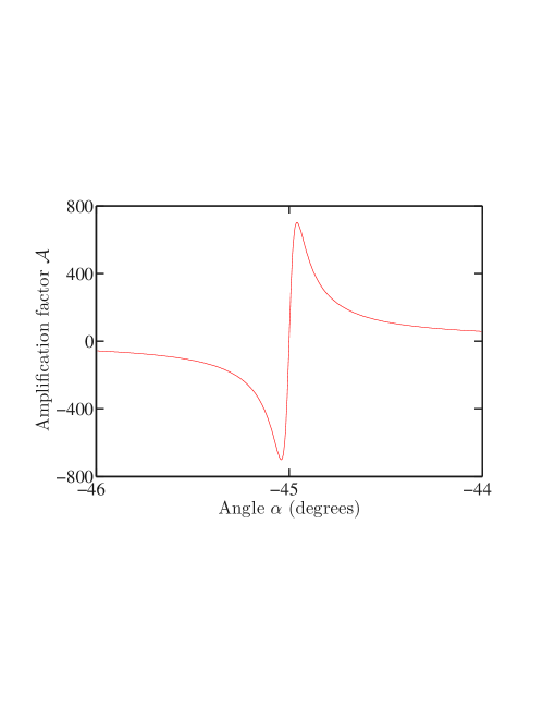
Fig. 1: Weak amplification of the displacement $\Delta$ as a function of the output polarization of the system (angle $\alpha)$. The phase difference is $\theta=0.01^{o}$. We consider displacements $\Delta=\Delta_{1}=-\Delta_{2}=10$ nm, and the beam waist is $w_{0}=10\mu$m.

2 Weak interference: general scenario

For the sake of simplicity, let us consider a simple case which shows the full potential of the scheme considered here. A linearly polarized input light beam with polarization $|\Psi_{in}\rangle=1/\sqrt{2}\,\left[|H\rangle+|V\rangle\right]$ and spatial shape $\Phi(x)$ propagates in a medium that couples the polarization and spatial degrees of freedom, thereby generating a polarization-dependent displacement of the photons, $\Delta_{1}$ and $\Delta_{2}$. The input state of the system (polarization) and the measuring device (position of the beam) can be written, up to a normalization constant, as

$$|in\rangle=|\Psi_{in}\rangle\otimes\int dx\,\Phi(x)|x\rangle.$$ (2)

The global state of the system and measuring device after the interaction writes [3]

$$|out\rangle=\int dx\left\{\Phi(x-\Delta_{1})|H\rangle+\Phi(x-\Delta_{2})\exp\left(i\varphi\right)|V\rangle\right\}|x\rangle,$$ (3)

where $\varphi$ stands for any polarization-dependent phase difference that can occur during the interaction. Finally, before being detected, the photons are projected into the polarization state $|\Psi_{out}\rangle=\cos\alpha|H\rangle+\exp(i\xi)\sin\alpha|V\rangle$. The intensity distribution of the output light beam can now be written as

$$I(x)=\left|\cos\alpha\,\Phi\left(x-\Delta_{1}\right)+\sin\alpha\,\Phi\left(x-\Delta_{2}\right)\exp\left(i\theta\right)\right|^{2},$$ (4)

with $\theta=\varphi-\xi$.

Let us assume that the light beam is Gaussian with beam waist $w_{0}$. Making use of the product theorem for Gaussian integrals [10], the mean value of the position of the beam, $\langle x\rangle=\int dx\,x\,I(x)/\int dx\,I(x)$ reads

$$\langle x\rangle=\frac{\Delta_{+}}{2}+\frac{\Delta_{-}}{2}\frac{\cos 2\alpha}{1+\gamma\sin 2\alpha\cos\theta},$$ (5)

where

$$\gamma=\exp\left[-\frac{\left(\Delta_{1}-\Delta_{2}\right)^{2}}{4w_{0}^{2}}\right],$$ (6)

$\Delta_{+}=\Delta_{1}+\Delta_{2}$ and $\Delta_{-}=\Delta_{1}-\Delta_{2}$. In all cases, $\Delta_{1},\Delta_{2}\ll w_{0}$, so $\gamma\sim 1$.

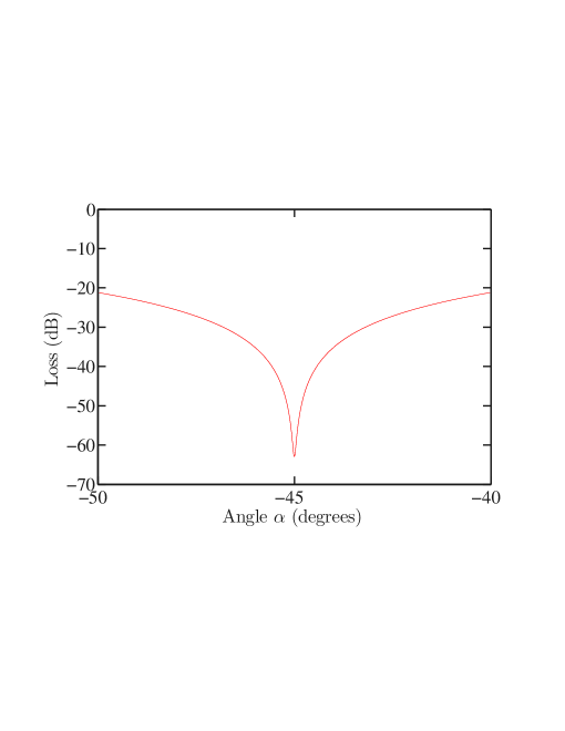
Fig. 2: Signal loss as a function of the angle $\alpha$ of the polarization of the output state. The phase difference is $\theta=0.01^{o}$, $\Delta_{1}=-\Delta_{2}=10$ nm and $w_{0}=10\mu$m.

Inspection of Eq. (5) shows that the value of $\Delta_{+}$ can not be amplified with the present scheme. In many experiments [2, 3], $\Delta_{1}=-\Delta_{2}$, so $\Delta_{+}=0$, and as a consequence the weak measurement amplifies all the relevant information. Therefore, the weak amplification happens for $\Delta_{-}$, with an amplification factor ${\cal A}$ that reads

$${\cal A}=\frac{\cos 2\alpha}{1+\gamma\sin 2\alpha\cos\theta}.$$ (7)

Fig. 1 shows the amplification factor for $\theta=0.01^{o}$. The maximum amplification takes place for the angle $\alpha_{0}=-1/2\,\sin^{-1}\left(\gamma\cos\theta\right)$, where the factor reaches the value of ${\cal A}_{max}=\left(1-\gamma^{2}\cos^{2}\theta\right)^{-1/2}$.

The loss of the system is given by

$$\frac{P_{out}}{P_{in}}=\frac{1}{2}\left[1+\gamma\cos\theta\sin 2\alpha\right],$$ (8)

where $P_{in,out}$ is the total input and output power of the optical beam, when integrated over all space. Fig. 2 shows the loss in the measurement expressed in dB, as $10\,\log(P_{out}/P_{in})$. Even though the enhancement of $\Delta$ can be a large staggering value for angles close to $-45^{o}$ (Fig. 1 shows an enhancement close to $10^{3}$), this is unfortunately accompanied by a severe loss penalty close to $70$ dB (Fig. 2). For instance, if the goal of the experiment is to attain a signal-to-noise ratio of 10 dB at the measurement stage, the input signal has to be correspondingly increased $70$ dB above this level.

As it can be seen in Eq. (7), the level of weak amplification achievable depends on the value of $\theta$, which should be chosen close to zero in order to achieve the maximum amplification. This angle can be modified by choosing the appropriate value $\xi$ of the polarization of the output state of the system. The power of the output signal also depends on this angle. Fig. (3) shows the signal loss for a few selected angles: $\alpha=-45^{o}$, $-30^{o}$, $0^{o}$ and $45^{o}$. In all cases, the loss goes from $\log\left[\left(1+\sin 2\alpha\right)/2\right]$ for $\theta=0$, to $-3$ dB for $\theta=\pm\pi/2$, which corresponds to post-selecting polarizations $\cos\alpha|H\rangle+\sin\alpha|V\rangle$ and $\cos\alpha|H\rangle+i\sin\alpha|V\rangle$, respectively. Importantly, the dependence of the losses on the polarization selected at the output for $\alpha\neq 0^{o},90^{o}$ is a consequence of the interference effect which is the essence of the weak measurement concept [8].

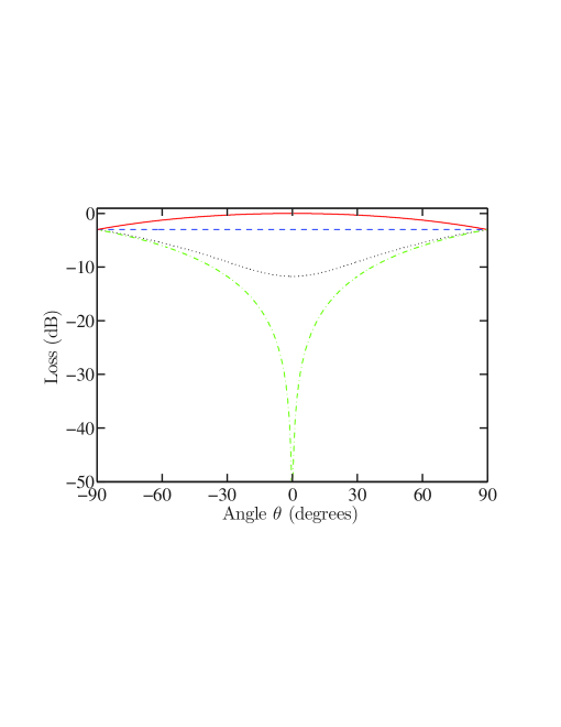
Fig. 3: Signal loss as a function of the angle $\theta$. The beam waist is $w_{0}=10\mu$m. Red solid line: $\alpha=45^{o}$; Blue dashed line: $\alpha=0^{o}$; Black dotted line: $\alpha=-30^{o}$; Green dotted dashed line: $\alpha=-45^{o}$.

3 Weak measurement in a high-signal regime

In the low-signal regime, when the input and output polarization states are quasi-orthogonal, the retrieval of information about the value of $\Delta$ comes with a severe loss penalty. But since the weak measurement is an interference phenomenon, we should be able, in principle, to observe interference also in the high-signal regime. In order to get information about the value of $\Delta$, we can measure the fractional loss $\Delta P/P_{in}$, where $\Delta P=P_{out}-P_{in}$. One obtains that

$$\frac{\Delta P}{P_{in}}=\frac{1}{2}\left[\gamma\cos\theta\sin 2\alpha-1\right].$$ (9)

Figure 4 shows the value of $\Delta P/P$ as a function of the spatial shift $\Delta$ for $\alpha=45^{o}$ and $\theta=0$, $0.1^{o}$, $0.2^{o}$ and $0.3^{o}$. The dependence of the fractional loss on $\Delta$ comes from the relationship between $\gamma$ and $\delta$, as given in Eq. (6). Notice that in all cases, the total losses of the system are below $3$ dB, which is significantly below the loss found in the usual regime of weak amplification, where losses can easily reach tens of dB for large amplifications. Moreover, in all cases shown in Fig. 4, the mean value of the beam position is $\langle x\rangle=0$, so the weak value concept does not convey any relevant information here.

The important point here is that by measuring the fractional loss, one can determine the value of the displacement $\Delta$. The maximum sensitivity of the scheme proposed is obtained for $\alpha=45^{o}$ and $\theta=0^{o}$. By choosing other values for these angles, one can decrease the fractional loss, making its detection easier. However, this would decrease the sensitivity, making the distinction between different spatial shifts $\Delta$ more difficult. Note that here we are assuming that there are not other sources of polarization-dependent losses.

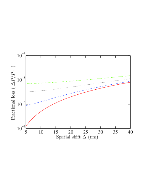
Fig. 4: Fractional loss $\Delta P/P$ as a function of the spatial shift $\Delta$. $\alpha=45^{o}$ and $w_{0}=10\mu$m. Red solid line: $\theta=0^{o}$; Blue dashed line: $\theta=0.1^{o}$; Black dotted line: $\theta=0.2^{o}$; Green dot-dashed line: $\theta=0.3^{o}$.

What is, in general, the minimum fractional loss measurable? In [11, 12], a high-frequency detection scheme for the detection of Raman gain in Stimulated Raman Scattering process was able to detect a fractional loss of the order of $\Delta P/P<10^{-7}$. The key point is to modulate the input signal at MHz rates to remove the low-frequency laser noise, implementing a detection scheme that is effectively shot-noise limited.

4 Conclusions

In conclusion, we have shown that since the idea of weak measurements is indeed an interference phenomenon, it is possible to obtain relevant information about the weak interaction of the physical system under study even in a regime where the signal is not depleted, and the concept of weak value does not convey any useful information. We demonstrate that we can measure tiny quantities generated during a weak interaction by detecting a measurable interference effect in the high-signal regime, as opposed to the usual case of weak amplification, which suffers from severe losses. Therefore, this widens the applicability of the weak measurement concept, allowing its use in a broader range of systems.

Finally, we should mention that even though we have discussed our ideas in the context of the specific case of polarization-dependent spatial shifts of optical beams, the main conclusions applies also to other systems, as well as to other degrees of freedom, i.e., frequency. Our scheme would also apply to systems in a higher-dimensional space, so that the total input state writes

$$|in\rangle=\frac{1}{\sqrt{n}}\sum_{i=1}^{n}|u_{i}\rangle\otimes\int dx\,\Phi(x)|x\rangle,$$ (10)

where $|u_{i}\rangle$ is a base of the N-dimensional space.

An example of this kind of interaction, where our system could be implemented, is the rotational Doppler frequency shift imparted to a beam with orbital angular momentum (OAM) when it traverses a rotating optical device which introduces a time-varying OAM-dependent phase shift, such as a rotating Dove prism. In this case, the spatial and frequency degrees of freedom are coupled [13, 14], so that the state of the light beam after traversing the rotating Dove prism is

$$|out\rangle=\sum_{m}\int d\omega\Phi(\omega+2m\Omega)|m\rangle|\omega\rangle$$ (11)

Now, the interaction introduces frequency shifts $\Delta_{m}=2m\Omega$, where $m$ is the OAM mode index.