Homogenization of a catalyst layer model for periodically distributed pore geometries in PEM fuel cells

Abstract

We formally derive an effective catalyst layer model comprising the reduction of oxygen for periodically distributed pore geometries. By assumption, the pores are completely filled with water and the surrounding walls consist of catalyst particles which are attached to an electron conducting microstructure. The macroscopic transport equations are established by a multi-scale approach, based on microscopic phenomena at the pore level, and serve as a first step toward future optimization of catalyst layer designs.

1 Introduction

The global economy is faced with a transition towards a renewable energy infrastructure. The optimization of energy efficient devices and the development of new and environmentally friendly strategies for the production of electrical energy are key issues in this context. One promising field in this direction is fuel cell research. In particular, polymer electrolyte fuel cells might become future power sources for portable devices and motorized transport because of their high energy densities and thermodynamic efficiency. However, a major proportion of voltage losses occurs in the cathode catalyst layer (CL) [10], thereby lowering the efficiency of the cell. High platinum (Pt) loadings are required to enhance the oxygen reduction reaction such that sufficient current densities are achieved. The long-term target is to reduce current platinum use by an order of magnitude. Consequently, optimization of CL design so as to reduce voltage losses and the amount of costly platinum is a central goal in polymer electrolyte membrane (PEM) fuel cell research, see [2]. The catalyst layer in PEM fuel cells is comprised of a complex multiphase porous structure. Normally, it is a three-phase random composite of open gas pores and carbon-supported Pt in which ionomer strands are embedded. Nanometer-size platinum particles, the catalyst, are supported on larger carbon (C) agglomerate particles which are excellent electronic conductors. Proton transport occurs from the anode towards the cathode catalyst layer through the PEM and ultimately, inside the CL, through the ionomer which consists of nano-thin pieces of polymer electrolyte membrane. Oxygen enters through the gas diffusion layer (GDL) and diffuses into the catalyst layer inside the gas phase, where the oxygen concentration decreases toward the catalyst particles (Pt). Electrochemical reactions preferentially occur at the interface between the catalyst particles and the electrolyte (i.e. the ionomer). Only catalyst particles that are simultaneously accessible to electrons, protons, and oxygen are electrochemically active. Strong non-equilibrium effects for gas-phase flows in small-scale confined geometries as well as liquid water generated from the electrochemical reaction

$$\begin{split}\frac{1}{2}{\rm O}_{2}+2{\rm H}^{+}+2e^{-}\quad\rightleftharpoons\quad{\rm H}_{2}{\rm O}\,,\end{split}$$ (1.1)

complicate an exact description of proton transport in the catalyst layer. So far, little is known about the influence of geometrical parameters such as porosity, pore size, and surface properties of the C-Pt phase on proton transport and macroscopic reaction rates. Hence, systematic optimization of these parameters requires physical and mathematical understanding of relevant phenomena. The recent developments of ultra-thin catalyst layers (UTCLs) such as 3M’s organic perylene whiskers, see for example [12], carbon nanotubes [28], or carbon produced by template techniques where the porosity is controlled by a silica matrix [1], call for models which reliably account for the influence of the pore geometry on the transport properties. In addition, these nano-scale geometries can be designed without ionomer. In this case, liquid water facilitates proton transport which is what we will study in this contribution. To date, merely volume averaging is applied to fixed geometries like spheres or cylinders, capitalizing radial symmetry under restricting and simplifying assumptions [10, 14]. Hence, the goal of this article is to provide an upscaled macroscopic description which consistently describes general geometries/designs of the catalyst layer with the help of a microscopic periodic reference cell. Such a generalization will serve as a promising extension for the description of the new ultra-thin catalyst layers, carbon nanotubes and general meso-porous materials designed by template techniques. In general, volume averaging approaches cannot treat nonlinear models and require the choice of an appropriate test volume whose size is not obvious. As a consequence, such averages are less rigorous than homogenization techniques like the two-scale convergence method, for example [3, 18]. Here, we employ formal periodic homogenization which is a multi-scale approach, see for example [7, 11]. It allows to formally obtain the effective macroscopic description (1.2) without technical a priori estimates, followed by a convergence analysis. This is a subtle point since the convergence of such reactions impose new difficulties and open questions for a rigorous analysis of such interface phenomena. From an analytical perspective, it is interesting to note that there exists an electro-osmotic flow problem in cylindrical channels of PEM that can be solved explicitly without numerical tools [8]. These solutions might be useful for test purposes of numerical approaches. However, such solutions lack the reaction kinetics at the boundaries of the domain as in catalyst layer pores. Let us briefly summarize the main result of this article. We derive effective macroscopic equations for a general cathode catalyst layer $\Omega\subset\mathbb{R}^{d}$ containing reactions on its phase interfaces $S^{c}$, as explained for a cylindrical pore in Section 2.1. The spatial dimension is denoted by $1\leq d\leq 3$. The relevant physical quantities (in dimensionless form) are the oxygen concentration $C_{O}$, the proton concentration $C_{+}$, and the electrostatic potential $\Phi$ while water flux is neglected. However, since no water is produced at the anode, the macroscopic model derived here describes also well anodic currents. The new contribution of this article is the systematic derivation of reference cell problems which reliably capture the characteristic pore geometry of the considered catalyst layer. Solutions of these reference cell problems define effective diffusion tensors for oxygen, $\hat{\rm D}^{O}$, for protons, $\hat{\rm D}^{+}$, an effective mobility tensor, $\hat{\rm M}^{+}$, and an effective electric permittivity tensor $\hat{\varepsilon}$, see Theorem 3.2 in Section 3. The new effective catalyst layer model reads (in dimensionless form) as follows

$$\begin{split}(\textrm{\bf Upscaled model:})\quad\begin{cases}-{\rm div}\left(\hat{\rm D}^{O}\nabla C_{O}\right)=\overline{\beta}_{O}(C_{+})^{n_{+}}(C_{O})^{n_{O}}\exp\left(-\alpha_{c}(\Phi-\Phi_{0})\right)\,,&\qquad\textrm{in }\Omega\,,\\ -{\rm div}\left(\hat{\rm D}^{+}\nabla C_{+}+C_{+}\hat{\rm M}^{+}\nabla\Phi\right)=\overline{\beta}_{+}(C_{+})^{n_{+}}(C_{O})^{n_{O}}\exp\left(-\alpha_{c}(\Phi-\Phi_{0})\right)\,,&\qquad\textrm{in }\Omega\,,\\ -{\rm div}\left(\hat{\varepsilon}(\lambda^{2},\gamma)\nabla\Phi\right)=pC_{+}+\rho_{s}\,,&\qquad\textrm{in }\Omega\,,\end{cases}\end{split}$$ (1.2)

where $p$ is the porosity, $\rho_{s}(x):=\frac{1}{\left|Y\right|}\int_{I}\sigma_{s}(x,y)\,do(y)$ represents an effective surface charge on the pore walls $I:=\partial Y^{1}\cap\partial Y^{2}$ for a given surface charge density $\sigma_{s}$, $\overline{\beta}_{O}:=\frac{i_{0}L\Lambda}{4e{\rm D}_{O}}$ and $\overline{\beta}_{+}:=\frac{i_{0}L\Lambda}{e{\rm D}_{+}}\,,$ are dimensionless numbers mediating the coupling to interfacial reactions, $L$ is the characteristic length of the catalyst layer, and the parameters $n_{+}$ and $n_{O}$ denote reaction orders. $\Lambda$ stands for the Lebesgue measure of the interface, i.e., $\Lambda:=\left|I\right|$, where $I$ is the pore-solid interface constituting the pores walls. The variable $\Phi_{0}$ denotes the standard (equilibrium) potential. The parameter $\lambda:=\frac{\lambda_{D}}{L}$ represents the dimensionless Debye length and $\gamma:=\frac{\epsilon^{s}}{\epsilon^{p}}$ is the dimensionless electric permittivity. The constants $\lambda_{D},\,\epsilon^{s}$ and $\epsilon^{p}$ stand for the Debye length $\lambda_{D}:=\left(\frac{\epsilon^{p}RT}{2z^{2}_{+}eF\overline{c}}\right)^{1/2}$, the electric permittivity of the solid and the pore phase, respectively. $\overline{c}$ denotes the reference salt concentration. The parameter $z_{+}$ is the charge number of the protons $C_{+}$. The new effective catalyst layer model (1.2) allows for similar limit considerations with respect to $\lambda$ and $\gamma$ as initiated in [24]. These convenient and advantageous limit properties of (1.2) are due to the generality of the homogenization procedure performed here. Since especially the thin-double-layer limit is a widely used approximation for the Poisson-Nernst-Planck system in engineering, we are able to compare related results in engineering with the systematically derived macroscopic system (1.2) by mathematical homogenization theory herein. As already stressed in [24], the effective Nernst-Planck equations agree very well with the heuristically suggested models in [13, 15, 22, 29]. We point out that the system (1.2) extends results from previous articles [24, 27] by including Butler-Volmer reactions on the solid/liquid interfaces in the pores. Due to the additional non-linearities arising in the coupled system (1.2), a careful fixed point iteration scheme is required to solve such a problem. Systematic strategies for the development of such schemes can be found in Jerome’s book [16] for instance. Several references exist in the literature which heuristically motivate effective (upscaled) equations for the catalyst layer that are sometimes close or similar to the new and mathematically derived formulation (1.2) in here, see for example [9, 10]. Hence this article strives to fill this gap with a systematic derivation. A different approach to the derivation in this contribution can be found in [20] where a non-equilibrium model, using statistical mechanics, is applied to compute effective friction and diffusion coefficients in Nafion membranes. Our work utilizes such computed coefficients at the pore level for the derivation of the new macroscopic equations (1.2) at the scale of the catalyst layer. Section 2.1 introduces the relevant equations for a single pore. In Section 2.2, a periodic representation of the catalyst layer provides the microscopic representation which is the starting point for the upscaled results which are presented in Section 3 and derived in Section 4.

2 Problem description

For the presentation of the main results, we first need to explain the problem of cathode catalyst layers in proton exchange membrane fuel cells (PEMFC) at the level of a single pore in Section 2.1 and then extend it to the whole catalyst layer described by a periodic representation of such single pores in Section 2.2.

2.1 Single pore model

We begin with equations describing a single water-filled pore. For simplicity, we restrict our analysis to the cathode catalyst layer. The analysis for the anode layer is then an immediate adaptation of our results. We first formulate a model for a single pore with boundary conditions defined by the physical fluxes as depicted in Figure 1. We are neglecting the flux of liquid water and assume the pore is uniformly filled with water.

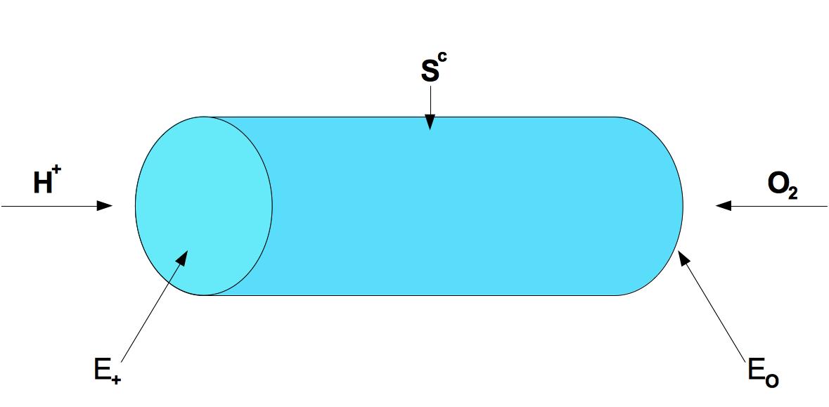
Figure 1: Single water-filled pore $\Omega^{p}$ in the cathode catalyst layer: Left entrance $E_{+}$: Flux of protons enters through the polymer electrolyte membrane (PEM). Cylinder wall $S^{c}$: Surface where the reaction takes place. It is the interface between the catalyst and the water-filled pore. Right entrance $E_{O}$: Flux of oxygen enters through the gas diffusion layer (GDL).

In order to place our considerations on a well-defined thermodynamic basis, we require that our physical quantities of interest, i.e., oxygen concentration $C_{O}$, proton concentration $C_{+}$, and electric potential $\Phi$, constitute the following dimensionless bulk free energy,

$$\begin{split}H(C_{O},C_{+},\Phi)=\frac{1}{RT}(U-TS)&:=\int_{\Omega}\left(\sum_{k\in\left\{O,+\right\}}C_{k}\left({\rm log}\,C_{k}-1\right)+C_{+}\Phi-\lambda^{2}\left|\nabla\Phi\right|^{2}\right)\,dx\,,\end{split}$$ (2.3)

where $U$ and $S$ represent the internal energy and the entropic contribution, respectively, and $\Phi:=\frac{z_{+}F\phi}{RT}=\frac{ez_{+}\phi}{kT}$ is the dimensionless electric potential. The free energy (2.3) allows us to define the chemical potentials $\mu_{O}(C_{O})$ and $\mu_{+}(C_{+},\Phi)$ associated with the catalytic pore governed by $C_{O}$ and $C_{+}$. These potentials are defined as the Fréchet derivative of $H$, that means,

$$\begin{split}\mu_{O}(C_{O})&:=\frac{\delta H}{\delta C_{O}}={\rm log}\,C_{O}\,,\\ \mu_{+}(C_{+},\Phi)&:=\frac{\delta H}{\delta C_{+}}={\rm log}\,C_{+}+\Phi\,.\end{split}$$ (2.4)

Motivated by Onsager [19], it is generally accepted that a thermodynamic system is driven by gradients of associated chemical potentials. Hence, we can define the fluxes $J_{O}$ and $J_{+}$ corresponding to (2.4) by

$$\begin{split}J_{O}&:=C_{O}k_{B}T{\rm M}^{O}\nabla\mu_{O}={\rm D}^{O}\nabla C_{O}\,,\\ J_{+}&:=C_{+}k_{B}T{\rm M}^{+}\nabla\mu_{+}={\rm D}^{+}\left(\nabla C_{+}+C_{+}\nabla\Phi\right)\,,\end{split}$$ (2.5)

where we applied Einstein’s relation ${\rm M}^{k}=\frac{D^{k}}{k_{B}T}$ for $k\in\left\{+,O\right\}$ and the identity $\frac{RT}{F}=\frac{kT}{e}$. We require that oxygen and proton concentrations are conserved quantities and hence satisfy the continuity equations,

$$\begin{split}\frac{\partial C_{O}}{\partial t}&={\rm div}\left(J_{O}\right)\,,\qquad\textrm{and}\qquad\frac{\partial C_{+}}{\partial t}={\rm div}\left(J_{+}\right)\,,\end{split}$$ (2.6)

where we made use of the diffusion timescale $\tau_{D}=\frac{\ell^{2}}{{\rm D}}$ for a characteristic length scale $\ell$. For simplicity, we continue our considerations with the time-invariant formulations of (2.6) and hence set $\frac{\partial C_{O}}{\partial t}=\frac{\partial C_{+}}{\partial t}=0$. We also neglect any possible source or sink terms in the bulk of the microscopic formulation. However, a major result of this article is the systematic derivation of such source and sink terms in the new upscaled catalyst layer model. Finally, we remark that the concentrations $C_{O}$ and $C_{+}$ are extended by zero in the solid phase and again denoted by $C_{+}$ and $C_{O}$ for notational convenience. This physically means that the solid phase is considered as an ideal conductor such that any charge accumulation is immediately equilibrated. The electric potential is defined on both solid and liquid phases by taking into account the different electric permittivities. Such a regularization is related to a diffuse interface approach and hence physically meaningful. Finally, we account for different electric permittivities in the pore and the solid phase by $\hat{\varepsilon}(x):=\lambda^{2}\chi_{\Omega^{p}}(x)+\gamma\chi_{\Omega\setminus\Omega^{p}}(x)$. Next, we move our focus from the bulk of the pore to the solid/liquid interface. Along the pore wall $S^{c}$, see Figure 1, we have to account for the reduction reaction of oxygen. This reaction, introduced in (1.1), is explained in detail in standard literature on electro-chemistry [17, 21]. We now derive a boundary condition on the pore wall related to this reaction. General electrode reactions can be formulated for reactants $S_{\iota}$, products $S_{j}$, and corresponding stoichiometric coefficients $\nu_{\iota}$ and $\nu_{j}$, respectively, by an abstract equation

$$\begin{split}\sum_{\iota}\nu_{\iota}S_{\iota}+ne^{-}\quad\rightleftharpoons\quad\sum_{j}\nu_{j}S_{j}\,,\end{split}$$ (2.7)

which can be transformed into an elementary charge transfer reaction as a one-electron reaction

$$\begin{split}\sum_{\iota}\frac{\nu_{\iota}}{n}S_{\iota}+e^{-}\quad\rightleftharpoons\quad\sum_{j}\frac{\nu_{j}}{n}S_{j}\,,\end{split}$$ (2.8)

where $n$ stands for the number of electrons. By choosing $S_{\iota_{1}}=O_{2}$, $\nu_{\iota_{1}}=\frac{1}{2}$, $S_{\iota_{2}}=H^{+}$, $\nu_{\iota_{2}}=2$, $S_{\iota_{3}}=e^{-}$, $\nu_{\iota_{3}}=n=2$, and $S_{j_{1}}=H_{2}O$ in (2.8), we recover (1.1) as the one-electron reaction

$$\begin{split}\frac{1}{4}O_{2}+H^{+}+e^{-}\quad\rightleftharpoons\quad\frac{1}{2}H_{2}O\,,\end{split}$$ (2.9)

see Figure 2. This allows to define the total electric current density through the pore walls by the Butler-Volmer equation

$$\begin{split}i=i_{0}\left[\prod_{\iota}\frac{{C}_{\iota}^{n_{red,\iota}}}{\overline{C}_{\iota}^{n_{red,\iota}}}\exp\left(\alpha_{a}\eta\right)-\prod_{j}\frac{C_{j}^{n_{ox,j}}}{\overline{C_{j}}^{n_{ox,j}}}\exp\left(-(1-\alpha_{a})\eta\right)\right]\,,\end{split}$$ (2.10)

where $i_{0}$ (of order $\left[\frac{Q}{\tau\ell^{2}}\right]$, with $Q$ denoting a reference charge, $\tau$ a characteristic time and $\ell$ a reference length) is the exchange current density defined by

$$\begin{split}\left|i_{0}\right|:=Fk_{a}^{*}\prod_{\iota}\overline{C}_{\iota}^{n_{red,\iota}}\exp\left(\alpha_{a}\Phi_{0}\right)=Fk_{c}^{*}\prod_{j}\overline{C}_{j}^{n_{ox,j}}\exp\left(-(1-\alpha_{a})\Phi_{0}\right)\,.\end{split}$$ (2.11)

The variable $\eta:=\Phi-\Phi_{0}$ is the over-potential and the parameter $\alpha_{a}$ is called anodic charge transfer coefficient. The densities $\overline{C}_{\iota}$ stand for the bulk concentrations of protons $\iota=+$ and oxygen $\iota=O$, respectively, $k^{*}_{a}$ and $k^{*}_{c}$ are the anodic and cathodic rate constants, respectively, and $\Phi_{0}$ denotes the Nernst equilibrium potential. Further, $n_{red,\iota}$ and $n_{ox,j}$ are the reaction orders of the $\iota$-th and $j$-th species, respectively.

Figure 2: Cathodic current $i_{c}$ (cathodic branch) defined as a half-cell reaction by a modification of the classical Nernst equation for the activation potential $\Phi$.

It is well-accepted in catalyst layer modeling to take the cathodic branch of the Butler-Volmer equation (2.10), see [10]. This approximation is justified at sufficiently large over-potentials $\eta=\Phi-\Phi_{0}$. Hence, this branch leads to a reaction rate of

$$\begin{split}R(C_{+},C_{O},\eta):=i_{0}C_{+}^{n_{+}}C_{O}^{n_{O}}\exp\left(-\alpha_{c}\eta\right)\,,\end{split}$$ (2.12)

for the cathodic transfer coefficient $\alpha_{c}:=1-\alpha_{a}$, the dimensionless concentrations $C_{+}$ and $C_{O}$, and the reaction orders $n_{+}=n_{+,ox}$ and $n_{O}=n_{O,ox}$. Note that we follow Chan and Eikerling [10] regarding the over-potential $\eta$ which assumes, in fact, only non-positive values. We remark that in electrochemistry one often calls $\Phi$ an activation over-potential in difference to the equilibrium potential $\Phi_{0}$. Let us summarize the relevant equations and refer the reader to Figure 1 for convenience:

Bulk equations for a single water-filled pore $\Omega^{p}$

Oxygen transport:

$$\begin{split}-\textrm{div}\,\,\left({\rm D}^{O}\nabla C_{O}\right)=0&\qquad\textrm{in }\Omega^{p}\,.\end{split}$$ (2.13)

Proton transport:

$$\begin{split}-\textrm{div}\,\,\left({\rm D}^{+}\left(\nabla C_{+}+C_{+}\nabla\Phi\right)\right)=0&\qquad\textrm{in }\Omega^{p}\,.\end{split}$$ (2.14)

Electric potential $\phi$:

$$\begin{split}-\lambda^{2}\Delta\Phi=C_{+}&\qquad\textrm{in }\Omega^{p}\,.\end{split}$$ (2.15)

Boundary conditions on the pore walls $\partial\Omega^{p}=E_{O}\cup E_{+}\cup S^{c}$

Right entrance of the pore $E_{O}$:

$$\begin{split}C_{O}=C^{D}_{O}&\qquad\textrm{on }E_{O},\\ -\nabla_{n}C_{+}-C_{+}\nabla_{n}\Phi=0&\qquad\textrm{on }E_{O}\,,\\ \Phi=\Phi^{D}_{O}&\qquad\textrm{on }E_{O}\,,\end{split}$$ (2.16)

Left entrance of the pore $E_{+}$:

$$\begin{split}-\nabla_{n}C_{O}=0&\qquad\textrm{on }E_{+}\,,\\ C_{+}=C_{+}^{D}&\qquad\textrm{on }E_{+}\,,\\ \Phi=\Phi^{D}_{H}&\qquad\textrm{on }E_{+}\,,\end{split}$$ (2.17)

Pore wall $S^{c}$:

$$\begin{split}-\nabla_{n}C_{O}=\frac{1}{4}R(C_{+},C_{O},\eta)&\qquad\textrm{on }S^{c}\,,\\ -\nabla_{n}C_{+}-C_{+}\nabla_{n}\Phi=R(C_{+},C_{O},\eta)&\qquad\textrm{on }S^{c}\,,\\ -\epsilon_{p}\nabla_{n}\Phi=\sigma_{s}(x)&\qquad\textrm{on }S^{c}\,.\end{split}$$ (2.18)

The surface charge density $\sigma_{s}$ is introduced in (1.2). The gradient $\nabla_{n}:={\bf n}\cdot\nabla$ is defined with respect to a normal vector ${\bf n}$ pointing outward of the pore domain $\partial\Omega^{p}$. We see that all protons that enter the domain are consumed at the wall while water is being produced. The latter process is neglected in this contribution so as to simplify the model. Strictly speaking, water flow needs to be included as an advective flux.

2.2 Microscopic, periodic catalyst layer

The porous catalyst layer $\Omega$ of characteristic length $L$ decomposes into a pore region $\Omega^{p}$ and a material domain $\Omega^{s}$, which represents carbon-supported platinum. The boundary $\partial\Omega^{p}=E_{O}\cup E_{+}\cup{\cal I}$ where $E_{+}$ denotes the left entrance (Fig. 1), $E_{O}$ the right entrance (Fig. 1), and ${\cal I}:=\partial\Omega^{p}\cap\partial\Omega^{s}$ the water/solid interface. Furthermore, we assume that the pores are periodically distributed in $\Omega$, see Figure 3. The heterogeneity of the periodic catalyst layer is defined by the parameter $r:=\frac{\ell}{L}$. We set $\ell=1$ and hence define a periodic unit pore $Y:=[0,\ell]^{d}$. The index set

$$\begin{split}K_{r}:=\left\{j\in\mathbb{Z}^{d}\,\Bigr{|}\,{\rm dist}\left(rj,\partial\Omega\right)<r\sqrt{d}\right\}\,,\end{split}$$ (2.19)

allows us to denote this pore distribution and the solid regions by

$$\begin{split}\Omega^{p}_{r}&:=\Omega\cap\bigcup_{z\in\mathbb{Z}^{d}\setminus K_{r}}r\left\{z+Y^{p}\right\}\,,\\ \Omega^{s}_{r}&:=\Omega\cap\bigcup_{z\in\mathbb{Z}^{d}\setminus K_{r}}r\left\{z+Y^{s}\right\}\,,\end{split}$$ (2.20)

respectively, where $Y^{p}\subset Y$ denotes the pore phase in the reference cell $Y$ and $Y^{s}\subset Y$ denotes the heterogeneous C-Pt (carbon nanotubes, carbon meso-pores) or polymer-Pt (3M’s UTCL) phase. In fact, $Y^{p}$ represents the single pore considered in the previous Section 2.1. Note that $\Omega^{p}$ differs from the periodic replacement $\Omega^{p}_{r}$ which is scaled by $r$. These conventions and assumptions enable us to rewrite the system (2.13)-(2.18) in the following dimensionless form

$$\begin{split}(\textrm{\bf Micro bulk model:})\quad\begin{cases}-\Delta C_{O}^{r}=0&\qquad\textrm{in }\Omega_{r}^{p}\,,\\ -\Delta C_{+}^{r}-\textrm{div}\,\left(C^{r}_{+}\nabla\Phi^{r}\right)=0&\qquad\textrm{in }\Omega^{p}_{r}\,,\\ -\textrm{div}\,\left({\varepsilon}\left(\frac{x}{r}\right)\nabla\Phi^{r}\right)=C_{+}^{r}&\qquad\textrm{in }\Omega\,,\end{cases}\end{split}$$ (2.21)

where $\varepsilon(x/r):=\lambda^{2}\chi_{\Omega^{p}_{r}}(x/r)+\gamma\chi_{\Omega^{s}_{r}}(x/r)$ is $Y$-periodic, and $C_{0}^{r},\,C_{+}^{r}$, and $\Phi^{r}$ satisfy the same boundary conditions on $E_{+}$ and $E_{O}$ as imposed in (2.16) and (2.17).

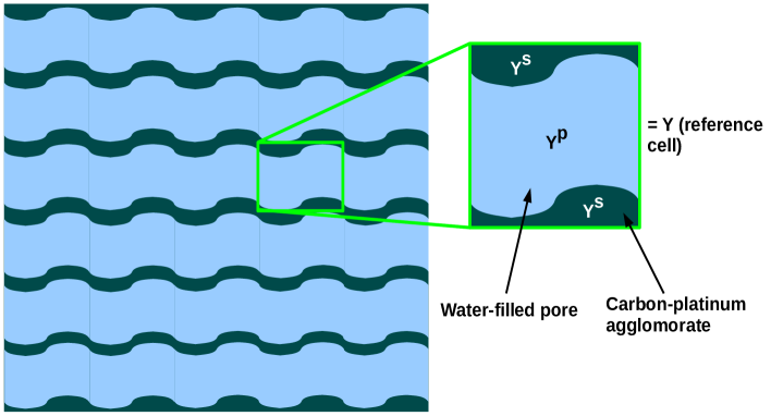
Figure 3: Left: Periodic array (with periodicity scaled by $r$) of water-filled pores $\Omega^{p}$ between thin catalytic layers $\Omega^{s}$ containing carbon supported platinum particles. Right: Reference cell characterizing the pore geometry.

On the interface ${\cal I}^{r}:=\partial\Omega^{p}_{r}\cap\partial\Omega_{r}^{s}$, which is denoted by $S^{c}$ in Figure 1 for the case of a single pore, we have the following boundary conditions

$$\begin{split}(\textrm{\bf Micro interface:})\quad\begin{cases}-\nabla_{n}C^{r}_{O}=r\beta_{O}(C_{O}^{r})^{n_{O}}(C_{+}^{r})^{n_{+}}{\rm exp}\left[-\alpha_{c}\left(\Phi^{r}-\Phi_{0}\right)\right]&\qquad\textrm{on }{\cal I}^{r}\,,\\ -\nabla_{n}C_{+}^{r}-C_{+}^{r}\nabla_{n}\Phi^{r}=r\beta_{+}(C_{O}^{r})^{n_{O}}(C_{+}^{r})^{n_{+}}{\rm exp}\left[-\alpha_{c}\left(\Phi^{r}-\Phi_{0}\right)\right]&\qquad\textrm{on }{\cal I}^{r}\,,\\ -{\varepsilon}(x/r)\nabla_{n}\Phi^{r}=r\sigma_{s}(x,x/r)&\qquad\textrm{on }{\cal I}^{r}\,,\end{cases}\end{split}$$ (2.22)

for the parameters $\beta_{O}:=\frac{i_{0}L}{4e{\rm D}_{O}}$ and $\beta_{+}:=\frac{i_{0}L}{e{\rm D}_{+}}$ both of dimension $[L^{-1}]$. We emphasize that the $(d-1)$-dimensional volume of the perforation surface ${\cal I}^{r}$ increases without bounds in the limit $r\to 0$. Therefore, problems with the boundary conditions on the perforation may show degeneration or unbounded growth of the solutions (depending on the sign of the coefficient in the Fourier condition). However, this phenomenon does not occur if the coefficient of the boundary operator asymptotically vanishes as the small parameter tends to zero, or has zero average over the perforation surface. Hence, we scale the right hand-sides in (2.22) by $r>0$.

3 Main results

Before we state the main result in this article, we need to introduce the following definition.

Definition 3.1.

(Local equilibrium) We say that the periodic reference cells $Y$ are in local thermodynamic equilibrium if and only if

$$\begin{split}\mu_{0}^{+}={\rm log}\,C_{+}(x)+\Phi(x)={\rm const.}\qquad\textrm{in }x/r=:y\in Y\,,\end{split}$$ (3.23)

where $\mu_{0}^{+}$ can only assume different values in different reference cells $Y$.

Subsequently, we employ the notation

$$\begin{split}{\mathcal{M}}_{U}(f):=\frac{1}{\left|U\right|}\int_{U}f\,dx\,,\end{split}$$ (3.24)

for arbitray $U\subset\mathbb{R}^{d}$ and summarize the main result of this article.

Theorem 3.2.

We assume that the periodic reference cells $Y:=Y^{p}\cup Y^{s}\subset\mathbb{R}^{d}$ are in local thermodynamic equilibrium, see Definition 3.1. Then, the microscopic problem (2.21)–(2.22) admits, for the formal asymptotic expansions

$$\begin{split}C_{O}^{r}(x)&\sim C_{O}^{0}(x)+rC_{O}^{1}(x,y)+r^{2}C_{O}^{2}(x,y)+\dots\,,\\ C_{+}^{r}(x)&\sim C_{+}^{0}(x)+rC_{+}^{1}(x,y)+r^{2}C_{+}^{2}(x,y)+\dots\,,\\ \Phi^{r}(x)&\sim\Phi^{0}(x)+r\Phi^{1}(x,y)+r^{2}\Phi^{2}(x,y)+\dots\,,\end{split}$$ (3.25)

the following leading order macroscopic system

$$\begin{split}(\textrm{\bf Upscaled model:})\quad\begin{cases}-{\rm div}\left(\hat{\rm D}^{O}\nabla C_{O}\right)=\overline{\beta}_{O}(C_{+})^{n_{+}}(C_{O})^{n_{O}}\exp\left(-\alpha_{c}(\Phi-\Phi_{0})\right)\,,&\qquad\textrm{in }\Omega\,,\\ -{\rm div}\left(\hat{\rm D}^{+}\nabla C_{+}+C_{+}\hat{\rm M}^{+}\nabla\Phi\right)=\overline{\beta}_{+}(C_{+})^{n_{+}}(C_{O})^{n_{O}}\exp\left(-\alpha_{c}(\Phi-\Phi_{0})\right)\,,&\qquad\textrm{in }\Omega\,,\\ -{\rm div}\left(\hat{\varepsilon}(\lambda^{2},\gamma)\nabla\Phi\right)=pC_{+}+\rho_{s}\,,&\qquad\textrm{in }\Omega\,,\end{cases}\end{split}$$ (3.26)

where $p:=\frac{\left|Y^{p}\right|}{\left|Y\right|}=\frac{\left|\Omega^{p}\right|}{\left|\Omega\right|}$ stands for the porosity. The effective porous media correctors $\hat{\rm D}^{+}=\left\{{\rm d}^{+}_{ik}\right\}_{1\leq i,k\leq d}$ , $\hat{\rm D}^{O}=\left\{{\rm d}^{O}_{ik}\right\}_{1\leq i,k\leq d}$ , $\hat{\rm M}^{+}=\left\{{\rm m}^{+}_{ik}\right\}_{1\leq i,k\leq d}$ , and $\hat{\varepsilon}=\left\{{\epsilon}^{0}_{kl}\right\}_{1\leq i,k\leq d}$ are defined for $\iota\in\left\{O,+\right\}$ by

$$\begin{split}{\rm d}^{\iota}_{ik}(t,x)&:=\frac{1}{\left|Y\right|}\int_{Y^{p}}\sum_{j=1}^{d}\left\{\delta_{ik}-\delta_{ij}\partial_{y_{j}}N^{k}_{\iota}(t,x,y)\right\}\,dy\,,\\ {\rm m}^{+}_{ik}&:=\frac{1}{\left|Y\right|}\int_{Y^{p}}\sum_{j=1}^{d}\left\{\delta_{ik}-\delta_{ij}\partial_{y_{j}}N^{k}_{\phi}(y)\right\}\,dy\,,\\ \epsilon^{0}_{ik}:&=\frac{1}{\left|Y\right|}\int_{Y}\sum_{j=1}^{d}{\varepsilon}(y)\left(\delta_{ik}-\delta_{ij}\partial_{y_{j}}N^{k}_{\phi}(y)\right)\,dy\,,\end{split}$$ (3.27)

and the integrands $N_{\iota}^{k}$ for $\iota\in\left\{+,O,\phi\right\}$ appearing in (3.27) solve the reference cell problems

$$\begin{split}N_{O}^{k}\,:\quad\begin{cases}\quad-{\rm div}_{y}\left(\nabla_{y}(N_{O}^{k}(y)-y_{k})\right)=0&\textrm{in }Y^{p}\,,\\ \quad\qquad{\rm n}_{I}\cdot\left(\nabla_{y}(N_{O}^{k}(y)-y_{k})\right)=0&\textrm{on }I:=\partial Y^{p}\,,\\ \qquad\quad N_{O}^{k}\textrm{ is $Y$-periodic and ${\mathcal{M}}_{Y^{p}}(N_{O}^{j})=0$}\,,\end{cases}\\ N_{+}^{k}\,:\quad\begin{cases}\quad-\Delta_{y}(N_{+}^{k}-y_{k})=-\Delta_{y}(N_{\phi}^{k}-y_{k})&\qquad\textrm{in }Y^{p}\,,\\ \qquad\qquad\left(-\nabla_{y}(N_{+}^{k}-y_{k})+\nabla_{y}(N_{\phi}^{k}-y_{k})\right)\cdot{\rm n}_{I}=0&\qquad\textrm{on }I:=\partial Y^{p}\,,\\ \qquad\qquad{N}_{+}^{k}\textrm{ is $Y$-periodic and ${\mathcal{M}}_{Y^{p}}(N_{+}^{k})=0$}\,,&\end{cases}\\ N_{\phi}^{k}\,:\quad\begin{cases}\quad-{\rm div}_{y}\left(\varepsilon(y)\nabla_{y}(N_{\phi}^{k}-y_{k})\right)=0&\qquad\textrm{in }Y\,,\\ \qquad\qquad N_{\phi}^{k}\textrm{ is $Y$-periodic and ${\mathcal{M}}_{Y}(N_{\phi}^{k})=0$}\,.&\end{cases}\end{split}$$ (3.28)

The dimensionless parameters $\overline{\beta}_{O}$ and $\overline{\beta}_{+}$ in (3.26) are defined by

$$\begin{split}\overline{\beta}_{O}:=\frac{i_{0}L\Lambda}{4e{\rm D}_{O}}\qquad\textrm{and}\qquad\overline{\beta}_{+}:=\frac{i_{0}Ll\Lambda}{e{\rm D}_{+}}\,,\end{split}$$ (3.29)

respectively, where $\Lambda:=\left|\partial Y^{p}\cap\partial Y^{s}\right|=\left|I\right|$. Finally, the surface charge $\sigma_{s}$ turns, through upscaling, into the background charge

$$\begin{split}\rho_{s}(x):=\frac{1}{\left|Y\right|}\int_{\partial Y^{p}}\sigma_{s}(x,y)do(y)\,,\end{split}$$ (3.30)

where $do$ denotes the $(d-1)$-dimensional surface measure.

Remark 1.

The boundary conditions imposed on the system (3.26) are canonical extensions of the boundary conditions from the single pore case (2.16)–(2.18) with no-flux conditions normal to solid walls on $\partial\Omega$.

Remark 2.

(Error estimates) Let us emphasize that in [25] one can find rigorous error estimates of the porous media Poisson-Nernst-Planck problem for no-flux boundary conditions instead of the Butler-Volmer reactions. For such a scenario, which additionally depends on time $t\geq 0$, the following result holds:

• Under suitable regularity assumptions one achieves that for $t,r>0$, and a generic constant $C>0$, the error ${\bf E}_{r}:=\tilde{\bf u}_{r}-({\bf u}_{0}+r{\bf u}_{1})$ between the exact solution $\tilde{\bf u}_{r}={\bf T}_{r}{\bf u}_{r}$ of the periodic formulation and its homogenized approximation ${\bf u}_{0}$ satisfies the following estimates

  $$\begin{split}\textrm{\bf(Error estimates)}\qquad\begin{cases}\quad\left\|{\rm E}^{1}_{r}\right\|_{L^{2}(\Omega)}^{2}(t)+\left\|{\rm E}^{2}_{r}\right\|_{L^{2}(\Omega)}^{2}(t)\leq C\left(r+r^{2}\right)t\,,&\\ \quad\left\|{\rm E}_{r}^{3}\right\|_{H^{1}(\Omega)}^{2}(t)\leq C\left(r+r^{2}\right)(t+1)\,,&\end{cases}\end{split}$$ (3.31)

  where ${\bf E}_{r}:=[{\rm E}^{1}_{r},{\rm E}^{2}_{r},{\rm E}^{3}_{r}]^{\prime}$, ${\bf u}_{0}:=[c_{+}^{0},c_{-}^{0},\phi^{0}]^{\prime}$, and ${\bf u}_{r}:=[c_{+}^{r},c_{-}^{r},\phi^{r}]^{\prime}$.

As one can see in (3.31), the time-dependence might impose additional sources for errors in the effective approximation. For a proof and more details we refer the interested reader to [25].

We briefly verify non-negativity of the proton concentration $C_{+}$ in (2.14). To this end, we introduce the following Auxiliary problem: Let $C_{+}$ solve

$$\begin{split}-{\rm div}\,\left({\rm D}^{+}\left(\nabla C_{+}+\left[C_{+}\right]^{+}\nabla\Phi\right)\right)=0\qquad\textrm{in }\Omega^{p}\,,\end{split}$$ (3.32)

where we define the regularization $[x]^{+}:=\sup\left\{0,x\right\}$ for $x\in\mathbb{R}$.

Lemma 3.

(Non-negativity) Concentrations $C_{+}$ of (3.32) are almost everywhere non-negative.

This immediately implies the non-negativity of $C_{+}$ for the original problem (2.14)₂. A corresponding derivation in the more general context of fluid flow can be found in [23].

Proof 3.3.

The definitions $[C_{+}]^{+}:=\sup\left\{C_{+},0\right\}$ and $[C_{+}]^{-}:=\sup\left\{-C_{+},0\right\}$ allow to multiply (3.32) by the test function $\xi=[c_{+}]^{-}$ such that after subsequent integration and integration by parts we obtain

$$\begin{split}&\left({\rm D}^{+}\nabla\left\{[C_{+}]^{+}-[C_{+}]^{-}\right\},\nabla[C_{+}]^{-}\right)+\left(\left[[C_{+}]^{+}-[C_{+}]^{-}\right]^{+}{\rm D}^{+}\nabla\Phi,\nabla[C_{+}]^{-}\right)=0\,,\end{split}$$ (3.33)

where we took advantage of the definitions $[C_{+}]^{+}$ and $[C_{+}]^{-}$. Since the terms $\left[[C_{+}]^{+}-[C_{+}]^{-}\right]^{+}$ and $[C_{+}]^{-}$ are zero on complementary sets, we end up with

$$\begin{split}-{\rm D}^{+}\|\nabla[C_{+}]^{-}\|^{2}_{L^{2}}\geq 0\,.\end{split}$$ (3.34)

Since all the terms in (3.34) are positive, we have $[C_{+}]^{-}=0$ a.e. in $\Omega$ and hence non-negativity of solutions of (3.32).

Via the proof of Lemma 3 it follows immediately that solutions to (3.26)₂ are non-negative if and only if

$$\begin{split}R_{eff}(C_{+},C_{O},\eta):=\beta_{+}(C_{+})^{n_{+}}(C_{O})^{n_{O}}\exp\left(-\alpha_{c}\eta\right)\geq 0\,,\end{split}$$ (3.35)

which follows with the non-negativity of $C_{O}$. The next result of the article is initiated in the context of porous media in [24]. We consider situations where the electrical double layers are thin compared to the mean catalyst layer size $L>0$. The thin-double-layer approximation is a well-accepted approximation in electrochemistry and engineering for systems based on the Nernst-Planck equations such as (3.26). This approximation consists mathematically of passing to the limit $\lambda:=\frac{\lambda_{D}}{L}\to 0$. However, one immediately recognizes that such a limit alone does not have much influence on the form of (3.26). Hence, we additionally take the limit $\gamma\to 0$, i.e., we assume that the porous matrix is insulating, see also [27].

Corollary 3.4.

(Thin double layers in pores) Let us assume that the solid phase of the catalyst layer forms an insulating matrix and we know the porosity $p$, effective diffusion tensors $\hat{\rm D}^{O}$ and $\hat{\rm D}^{+}$, and the homogenized surface charge $\rho_{s}$. Then, the leading order bulk approximation for oxygen concentration $C_{O}$, proton concentration $C_{+}$, and electric potential $\Phi$ reads

$$\begin{split}\begin{cases}\quad-{\rm div}\left(\hat{\rm D}^{O}\nabla C_{O}\right)=\beta_{O}\left(-\frac{\rho_{s}}{p}\right)^{n_{+}}(C_{O})^{n_{O}}\exp\left(-\alpha_{c}(\Phi-\Phi_{0})\right)\,,\\ \quad-{\rm div}\left(\frac{\rho_{s}}{p}\hat{\rm D}^{+}\nabla\Phi\right)=\beta_{+}\left(-\frac{\rho_{s}}{p}\right)^{n_{+}}(C_{O})^{n_{O}}\exp\left(-\alpha_{c}(\Phi-\Phi_{0})\right)-{\rm div}\left(\hat{\rm D}^{+}\nabla\frac{\rho_{s}}{p}\right)\,,\\ \quad C_{+}=-\frac{\rho_{s}}{p}\,.\end{cases}\end{split}$$ (3.36)

We immediately recognize that (3.36) is different from thin-double-layer approximations of classical Nernst-Planck-Poisson systems since we do not have counter ions $C_{-}$ leading to the well-known quasi-electroneutrality in the electrolyte. Therefore, the electric potential solves now a nonlinear Poisson equation due to the upscaled interfacial reactions.

4 Formal derivation of the upscaled system (3.26) by the multiple-scale method

We assume that the periodic formulation (2.21)–(2.22) is well posed and immediately derive the homogenized problem via the multiple-scale method. We look for solutions in the form of the two-scale asymptotic expansions

$$\begin{split}C_{O}^{r}(x)&\sim C_{O}^{0}(x)+rC_{O}^{1}(x,y)+r^{2}C_{O}^{2}(x,y)+\dots\,,\\ C_{+}^{r}(x)&\sim C_{+}^{0}(x)+rC_{+}^{1}(x,y)+r^{2}C_{+}^{2}(x,y)+\dots\,,\\ \Phi^{r}(x)&\sim\Phi^{0}(x)+r\Phi^{1}(x,y)+r^{2}\Phi^{2}(x,y)+\dots\,,\end{split}$$ (4.37)

where functions are periodic with respect to the microscopic coordinate $y:=x/r$. We emphasize that the ansatz (4.37) is only formal since the convergence is not guaranteed and possible boundary layers are neglected. Moreover, we already took into account that the leading order terms are independent of the microscale $y$, see [24, 27] for instance. The following identities

$$\begin{split}\frac{\partial\varphi(x,y)}{\partial x_{i}}&=\partial_{x_{i}}\varphi(x,y)+\frac{1}{r}\partial_{y_{i}}\varphi(x,y)\,,\\ \frac{\partial^{2}\varphi(x,y)}{\partial x^{2}_{i}}&=\partial^{2}_{x_{i}}\varphi(x,y)+\frac{1}{r}\left(\partial_{x_{i}}\partial_{y_{i}}+\partial_{y_{i}}\partial_{x_{i}}\right)\varphi(x,y)+\frac{1}{r^{2}}\partial^{2}_{y_{i}}\varphi(x,y)\,,\end{split}$$ (4.38)

are an immediate consequence of the definition of the small scale variable $y$. After substituting (4.37)₁ into (2.21)₁ and collecting terms of equal power in $r$, we obtain a recurrent sequence of problems. The first has the form

$$\begin{split}-\sum_{k,j=1}^{d}\partial_{y_{k}}\left(\delta_{kj}\partial_{y_{j}}C_{O}^{1}\right)-\sum_{k,j=1}^{d}\partial_{x_{k}}\left(\delta_{k,j}\partial_{y_{j}}C_{O}^{0}\right)=0&\qquad\textrm{in }Y^{p}\,,\\ -\nabla_{y_{n}}C_{O}^{1}-\nabla_{x_{n}}C_{O}^{0}=0&\qquad\textrm{on }{\cal I}^{r}\cap Y\,,\end{split}$$ (4.39)

where $x\in\Omega$ plays the role of a parameter. An integral identity corresponding to problem (4.39) reads for all $V\in H^{1}_{\#}(Y^{p})$

$$\begin{split}\sum_{k,j=1}^{d}\int_{Y^{p}}\delta_{kj}\partial_{y_{j}}C_{O}^{1}\partial_{y_{k}}V\,dy&+\sum_{k,j=1}^{d}\int_{Y^{p}}\delta_{kj}\partial_{x_{j}}C_{O}^{0}\partial_{y_{k}}V\,dy=0\,.\end{split}$$ (4.40)

This equation suggests to choose $C_{O}^{1}$ as

$$\begin{split}C_{O}^{1}(x,y)=-\sum_{i=1}^{d}N_{O}^{i}(y)\partial_{x_{i}}C_{O}^{0}(x)\,.\end{split}$$ (4.41)

By inserting (4.41) into (4.40), we obtain the following problem for $N_{O}^{j}(y)$ and $1\leq j\leq d$, i.e.,

$$\begin{split}\partial_{x_{j}}C_{O}^{0}(x)\sum_{k,l=1}^{d}\left\{\int_{Y^{p}}\delta_{kl}\partial_{y_{l}}N_{O}^{j}(y)\partial_{y_{k}}V\,dy-\sum_{k=1}^{d}\int_{Y^{p}}\delta_{kj}\partial_{y_{k}}V\,dy\right\}=0\,.\end{split}$$ (4.42)

In the classical formulation, (4.42) reads

$$\begin{split}\begin{cases}\quad-{\rm div}_{y}\left(\nabla_{y}(N_{O}^{j}(y)-y_{j})\right)=0&\textrm{in }Y^{p}\,,\\ \quad\qquad{\rm n}_{I}\cdot\left(\nabla_{y}(N_{O}^{j}(y)-y_{j})\right)=0&\textrm{on }I:=\partial Y^{p}\,,\\ \qquad\quad N_{O}^{j}\textrm{ is $Y$-periodic and ${\mathcal{M}}_{Y^{p}}(N_{O}^{j})=0$}\,.\end{cases}\end{split}$$ (4.43)

We note that the last line in (4.43) is imposed in order to account for the fact that $N^{i}_{O}$ is only determined up to an additive constant. The next problem in the recurrent chain has the form

$$\begin{split}-\sum_{k,j=1}^{d}\partial_{y_{k}}\left(\delta_{kj}\partial_{y_{j}}C_{O}^{2}(x,y)\right)-\sum_{k,j=1}^{d}\partial_{x_{k}}\left(\delta_{kj}\partial_{y_{j}}C_{O}^{1}(x,y)\right)\quad\qquad\qquad\qquad&\\ -\sum_{k,j=1}^{d}\partial_{y_{k}}\left(\delta_{kj}\partial_{x_{j}}C_{O}^{1}(x,y)\right)-\sum_{k,j=1}^{d}\partial_{x_{k}}\left(\delta_{kj}\partial_{x_{j}}C_{O}^{0}(x)\right)=0\,,&\qquad\textrm{in }Y^{p}\,,\\ -\nabla_{y_{n}}C_{O}^{2}-\nabla_{x_{n}}C_{O}^{1}=\beta_{O}(C_{+}^{0})^{n_{+}}(C_{O}^{0})^{n_{O}}{\rm exp}\left[-\alpha_{c}\left(\Phi^{0}-\Phi_{0}\right)\right]\,\,,\,&\qquad\textrm{on }{\cal I}^{r}\cap Y\,.\end{split}$$ (4.44)

The integral formulation of (4.44) reads

$$\begin{split}&\sum_{k,j=1}^{d}\int_{Y^{p}}\delta_{kj}\partial_{y_{j}}C_{O}^{2}\partial_{y_{k}}V\,dy-\sum_{k,j=1}^{d}\int_{Y^{p}}\delta_{kj}\partial_{x_{k}}\left(\partial_{y_{j}}C_{O}^{1}\right)V\,dy+\sum_{k,j=1}^{d}\int_{Y^{p}}\delta_{kj}\partial_{x_{j}}C_{O}^{1}\partial_{y_{k}}V\,dy\\ &-\sum_{k,j=1}^{d}\int_{Y^{p}}\delta_{kj}\partial_{x_{k}}\left(\partial_{x_{j}}C_{O}^{0}\right)V\,dy-\sum_{k,j=1}^{d}\int_{{\cal I}^{r}\cap Y}\beta_{O}(C_{+}^{0})^{n_{+}}(C_{O}^{0})^{n_{O}}{\rm exp}\left[-\alpha_{c}\left(\Phi^{0}-\Phi_{0}\right)\right]V\,d\sigma(y)=0\,.\end{split}$$ (4.45)

The second and third term in (4.45) can be rewritten by (4.41) as

$$\begin{split}-\sum_{k,j=1}^{d}\int_{Y^{p}}\delta_{kj}\partial_{y_{j}}C_{O}^{1}\partial_{x_{k}}V\,dy&=-\sum_{k,j=1}^{d}\int_{Y^{p}}\delta_{kj}\partial_{y_{j}}N_{O}^{i}(y)\partial_{x_{i}}C_{O}^{0}(x)\partial_{x_{k}}V\,dy\,,\\ \sum_{k,j=1}^{d}\int_{Y^{p}}\delta_{kj}\partial_{x_{j}}C_{O}^{1}\partial_{y_{k}}V\,dy&=\sum_{k,j=1}^{d}\int_{Y^{p}}\delta_{kj}N_{O}^{i}(y)\partial_{x_{i}}\partial_{x_{j}}C_{O}^{0}(x)\partial_{y_{k}}V\,dy\,.\end{split}$$ (4.46)

The solvability condition for problem (4.45) is an equation for $C_{O}^{0}(x)$. It is the required homogenized (limit) equation. By defining

$$\begin{split}{\rm d}^{O}_{ik}&:=\sum_{j=1}^{d}\int_{Y^{p}}\left(-\delta_{ij}\frac{\partial N^{k}_{O}(y)}{\partial y_{j}}+\delta_{ik}\right)\,dy\,,\\ \Lambda&:=\left|\partial Y^{p}\cap\partial Y^{s}\right|\,,\end{split}$$ (4.47)

and after setting $V\equiv 1$ in (4.45), we end up with the homogenized equation

$$\begin{split}-\sum_{k,j=1}^{d}\partial_{x_{k}}\left({\rm d}^{O}_{kj}\partial_{x_{j}}C_{O}^{0}\right)=\overline{\beta}_{O}(C_{+}^{0})^{n_{+}}(C_{O}^{0})^{n_{O}}{\rm exp}\left[-\alpha_{c}\left(\Phi^{0}-\Phi_{0}\right)\right]\,,\end{split}$$ (4.48)

where $\overline{\beta}_{O}:=\Lambda\beta_{O}$ is dimensionless with $\beta_{O}$ defined after (2.22). The important information gained by the calculation of (4.48) is how the boundary condition (2.22)₁ enters in the upscaled or homogenized problem. Since the equation (2.21)₂ satisfies the same type of boundary condition on the interface as (2.21)₁, we take over the result from (4.48). Moreover, in view of the two-scale convergence analysis from [26], the macroscopic equations for the remaining two equations in (2.21) immediately turn into

$$\begin{split}\begin{cases}\quad-{\rm div}\left(\hat{\rm D}^{+}\nabla C^{0}_{+}+C^{0}_{+}\hat{\rm M}^{+}\nabla\Phi^{0}\right)=\overline{\beta}_{+}(C_{+}^{0})^{n_{+}}(C_{O}^{0})^{n_{O}}{\rm exp}\left[-\alpha_{c}\left(\Phi^{0}-\Phi_{0}\right)\right]&\qquad\textrm{in }\Omega\,,\\ \quad-{\rm div}\left(\hat{\varepsilon}\left(\lambda^{2},\gamma\right)\nabla\Phi^{0}\right)=pC_{+}^{0}&\qquad\textrm{in }\Omega\,,\end{cases}\end{split}$$ (4.49)

where $\overline{\beta}_{+}:=\Lambda\beta_{+}$ for $\beta_{+}$ defined after (2.22). Further, the correction tensors $\hat{\rm D}^{\iota}:=\left\{{\rm d}^{\iota}_{ik}\right\}_{1\leq i,k\leq d}$, $\hat{\rm M}^{+}:=\left\{{\rm m}^{+}_{ik}\right\}_{1\leq i,k\leq d}$, and $\hat{\varepsilon}:=\left\{\varepsilon^{0}_{ik}\right\}_{1\leq i,k\leq d}$ are defined by

$$\begin{split}{\rm d}^{\iota}_{ik}:=\frac{1}{\left|Y\right|}\sum_{j=1}^{d}\int_{Y^{p}}\left\{\delta_{ik}-\delta_{ij}\partial_{y_{j}}N_{\iota}^{k}(y)\right\}\,dy\qquad\forall i,k=1,\dots,N\,,\\ {\rm M}^{+}_{ik}:=\frac{1}{\left|Y\right|}\sum_{j=1}^{d}\int_{Y^{p}}\left\{\delta_{ik}-\delta_{ij}\partial_{y_{j}}N_{\phi}^{k}(y)\right\}\,dy\qquad\forall i,k=1,\dots,N\,,\\ \epsilon^{0}_{ik}:=-\frac{1}{\left|Y\right|}\sum_{j=1}^{d}\int_{Y}\left\{\varepsilon(y)\left(\delta_{ik}-\delta_{ij}\partial_{y_{j}}N_{\phi}^{k}\right)\right\}\,dy\qquad\forall i,k=1,\dots,N\,,\end{split}$$ (4.50)

for $\gamma:=\frac{\varepsilon_{s}}{\varepsilon_{p}}$, $\lambda:=\sqrt{\frac{\varepsilon_{p}RT}{2z_{+}^{2}eFC_{0}}}/L$, and $\iota\in\left\{+,O\right\}$. The correctors $N^{k}_{+}$ and $N^{k}_{\phi}$ solve the following reference cell problems

$$\begin{split}\begin{cases}\quad-\Delta_{y}(N_{+}^{k}-y_{k})=-\Delta_{y}(N_{\phi}^{k}-y_{k})&\qquad\textrm{in }Y^{p}\,,\\ \qquad\qquad\left(-\nabla_{y}(N_{+}^{k}-y_{k})+\nabla_{y}(N_{\phi}^{k}-y_{k})\right)\cdot{\rm n}_{I}=0&\qquad\textrm{on }I:=\partial Y^{p}\,,\\ \qquad\qquad{N}_{+}^{k}\textrm{ is $Y$-periodic and ${\mathcal{M}}_{Y^{p}}(N_{+}^{k})=0$}\,,&\\ \quad-{\rm div}_{y}\left(\varepsilon(y)\nabla_{y}(N_{\phi}^{k}-y_{k})\right)=0&\qquad\textrm{in }Y\,,\\ \qquad\qquad N_{\phi}^{k}\textrm{ is $Y$-periodic and ${\mathcal{M}}_{Y}(N_{\phi}^{k})=0$}\,.&\end{cases}\end{split}$$ (4.51)

The reference cell problems (4.43), (4.50), and (4.51), written in classical form, are mathematically only meaningful in the distributional sense. Existence and uniqueness follows then by Lax-Milgram’s theorem for a suitable weak formulation. For rigorous solvability results we refer the interested reader to [24, 26, 27]. As a consequence, it is suggested to apply Galerkin schemes (e.g. finite elements) for the computation of numerical solutions. We note that (1.2), which is obtained from the results in this section by dropping the superscript “0” in (4.48) and (4.49), can immediately be extended to account for a surface charge density $\sigma_{s}$ on the pore walls denoted by ${\cal I}$. Such a density enters on the right hand side in the third equation of the effective model (1.2) as the background charge

$$\begin{split}\rho_{s}(x):=\frac{1}{\left|\partial Y^{p}\right|}\int_{Y}\sigma_{s}(x,y)do(y)\,,\end{split}$$ (4.52)

see [4, 24] for a derivation. We promote this idea as a straightforward way to account for double layer effects without going into details of Stern or Helmholtz layers, see [6, 21] for an overview of such models and [9, 10] for applications. Here, the use of a surface charge is appropriate since (1.2) is time-independent and hence models the steady case where the double layers are in local thermodynamic equilibrium. In future work, we will apply our algorithm and methodology to a number of examples, especially 3M’s nano-structured thin-film catalyst layers.

5 Application to straight channels

Figure 4: A periodic catalyst layer defined by a single reference cell $Y:=[0,1]^{2}$ scaled by $r$. The variable $\rho_{s}$ denotes the effective surface charge at the pore-solid interface. $x_{3}$ is pointing out of the plane.

Auriault and Lewandowska [5] considered the situation of a porous medium defined by a periodic array of straight channels as depicted in Figure 4. They analytically compute a correction tensor in order to define a homogenized diffusion coefficient in porous structures. We make use of their results herein and hence restrict ourselves to the case of an insulating porous matrix, i.e., $\gamma\to 0$. Then, we obtain

$$\begin{split}\hat{\rm D}^{O}=\hat{\rm M}^{+}=\left[\begin{matrix}p&0&0\\ 0&0&0\\ 0&0&p\end{matrix}\right]\qquad\textrm{and}\qquad\hat{\varepsilon}=\left[\begin{matrix}p\lambda^{2}&0&0\\ 0&0&0\\ 0&0&p\lambda^{2}\end{matrix}\right]\,,\end{split}$$ (5.53)

where $p$ denotes the porosity and the zero-entry on the diagonal is the direction orthogonal to the direction of the channel, see Figure 4. Under (5.53) the macroscopic catalyst layer model becomes in the two-dimensional case

$$\begin{split}(\textrm{\bf Straight channel:})\quad\begin{cases}-p\left(\frac{\partial^{2}}{\partial x_{1}^{2}}+\frac{\partial^{2}}{\partial x_{3}^{2}}\right)C_{O}=\overline{\beta}_{O}(C_{+})^{n_{+}}(C_{O})^{n_{O}}\exp\left(-\alpha_{c}(\Phi-\Phi_{0})\right)\,,&\qquad\textrm{in }\Omega\,,\\ -p\left(\frac{\partial^{2}}{\partial x_{1}^{2}}+\frac{\partial^{2}}{\partial x_{3}^{2}}\right)C_{+}-p\frac{\partial}{\partial x_{1}}\left(C_{+}\frac{\partial}{\partial x_{1}}\Phi\right)-p\frac{\partial}{\partial x_{3}}\left(C_{+}\frac{\partial}{\partial x_{3}}\Phi\right)\\ \qquad\qquad\qquad\qquad\,\,\,=\overline{\beta}_{+}(C_{+})^{n_{+}}(C_{O})^{n_{O}}\exp\left(-\alpha_{c}(\Phi-\Phi_{0})\right)\,,&\qquad\textrm{in }\Omega\,,\\ -p\lambda^{2}\left(\frac{\partial^{2}}{\partial x_{1}^{2}}+\frac{\partial^{2}}{\partial x_{3}^{2}}\right)\Phi=pC_{+}+\rho_{s}\,,&\qquad\textrm{in }\Omega\,.\end{cases}\end{split}$$ (5.54)

The coordinate $x_{2}$ acts like a parameter in the system (5.54). We recover the results from [5] if we set $\Phi=0$ and $\overline{\beta}_{+}=\overline{\beta}_{O}=0$. Next, we want to apply the scenario of straight channels to the thin-double-layer approximation (3.36). As in (5.54), we consider an insulating porous matrix. We immediately end up with

$$\begin{split}\begin{cases}\quad-p\left(\frac{\partial^{2}}{\partial x_{1}^{2}}+\frac{\partial^{2}}{\partial x_{3}^{2}}\right)C_{O}=\overline{\beta}_{O}\left(-\frac{\rho_{s}}{p}\right)^{n_{+}}(C_{O})^{n_{O}}\exp\left(-\alpha_{c}(\Phi-\Phi_{0})\right)\,,\\ \quad-\frac{\partial}{\partial x_{1}}\left(\rho_{s}\frac{\partial}{\partial x_{1}}\Phi\right)-\frac{\partial}{\partial x_{3}}\left(\rho_{s}\frac{\partial}{\partial x_{3}}\Phi\right)=\overline{\beta}_{+}\left(-\frac{\rho_{s}}{p}\right)^{n_{+}}(C_{O})^{n_{O}}\exp\left(-\alpha_{c}(\Phi-\Phi_{0})\right)-\left(\frac{\partial^{2}}{\partial x_{1}^{2}}+\frac{\partial^{2}}{\partial x_{3}^{2}}\right)\rho_{s}\,,\\ \quad C_{+}=-\frac{\rho_{s}}{p}\,,\end{cases}\end{split}$$ (5.55)

where the coordinate $x_{2}$ acts again like a parameter. It is interesting to see that the porosity parameter $p$ cancels out in (5.55)₂ except for the reaction term. In future work, we will extend the upscaled equations towards fluid flow and compute effective transport coefficients based on the formulas (3.27) and (3.28) for carbon nanotubes [28] and UTCLs such as 3M’s organic perylene whiskers [12]. The first author acknowledges the support by the Swiss National Science Foundation (SNSF) through the grant PBSKP2-12459/1 during his stay at MIT and the second author the support by an NSERC Discovery Grant.

References

• [1] New Carbon Based Materials for Electrochemical Energy Storage Systems : Batteries , Supercapacitors and Fuel Cells. In Igor V. Barsukov, Christopher S. Johnson, Joseph E. Doninger, and Vyacheslav Z. Barsukov, editors, New Carbon Based Materials for Electrochemical Energy Storage Systems. Springer, 2003.
• [2] Annual progress report - U.S. Department of Energy - Hydrogen Program. Technical report, 2008.
• [3] G. Allaire. Homogenization and two-scale convergence. SIAM Journal of Mathematical Analysis, 23(6):1482–1518, 1992.
• [4] G. Allaire, A. Damlamian, and U. Hornung. Two-scale convergence on periodic surfaces and applications. In A. et al. Bourgeat, editor, Proceedings of the International Conference on Mathematical Modelling of Flow through Porous Media (May 1995), pages 15–25, Singapore, 1996. World Scientific Pub.
• [5] J.-L. Auriault and J. Lewandowska. Effective Diffusion Coefficient: From Homogenization to Experiment. Transport in Porous Media, 27(2):205–223, 1997.
• [6] A. Bard and L. Faulkner. Electrochemical Methods, Fundamentals and Applications. John Wiley & Sons, New Jersey, 2001.
• [7] A. Bensoussans, J.-L. Lions, and G. Papanicolaou. Analysis for Periodic Structures. North-Holland Publishing Company, North-Holland, Amsterdam, 1978.
• [8] P. Berg and J. Findlay. Analytical solution of PNP-Stokes equations in a cylindrical channel. Proc. Roy. Soc. A, 467:3157–3169, 2011.
• [9] P. M. Biesheuvel, Y. Fu, and M. Z. Bazant. Diffuse charge and Faradai reactions in porous electrodes. preprint, 2011.
• [10] K. Chan and M. Eikerling. A Pore-Scale Model of Oxygen Reduction in Ionomer-Free Catalyst Layers of PEFCs. Journal of The Electrochemical Society, 158(1):B18, 2011.
• [11] D. Cioranescu and P. Donato. An introduction to homogenization. Oxford University Press, 2000.
• [12] M. K. Debe, A. K. Schmoeckel, G. D. Vernstrom, and R. Atanasoski. High voltage stability of nanostructured thin film catalysts for PEM fuel cells. Journal of Power Sources, 161:1002–1011, 2006.
• [13] E. V. Dydek, B. Zaltzmann, I. Rubinstein, D. S. Deng, A. Mani, and M. Z. Bazant. Overlimiting current in a microchannel. submitted, 2011.
• [14] M. Eikerling, K. Malek, and Q. Wang. Catalyst Layer Modeling: Structure, Properties and Performance. In Jiujun Zhang, editor, PEM fuel cell electrocatalysis and catalyst layer: Fundamentals and Applications. Springer, 2008.
• [15] Y. He, D. Gillespie, D. Boda, I. Vlassiouk, R. S. Eisenberg, and Z. S. Siwy. Tuning transport properties of nanofluidic devices with local charge inversion. Journal of the American Chemical Society, 131(14):5194–5202, April 2009.
• [16] J. W. Jerome. Analysis of charge transport - a mathematical study of semiconductor devices. Springer, 1996.
• [17] J. S. Newman and K. E. Thomas-Alyea. Electrochemical systems. Wiley-IEEE, 2004.
• [18] G. Nguetseng. A general convergence result related to the theory of homogenization. SIAM Journal of Mathematical Analysis, 20(3):608–623, 1989.
• [19] L. Onsager. Reciprocal relations in irreversible processes I. Physical Review, 37, 1931.
• [20] S. J. Paddison, R. Paul, and T. Zawodzinski. Proton friction and diffusion coefficients in hydrated polymer electrolyte membranes: Computations with a non-equilibrium statistical mechanical model. The Journal of Chemical Physics, 115(16):7753, 2001.
• [21] W. Plieth. Electrochemistry for Materials Science. Elsevier, 2008.
• [22] P. Ramirez, S. Mafe, V. M. Aguilella, and A. Alcaraz. Synthetic nanopores with fixed charges : An electrodiffusion model for ionic transport. Physical Review E, 68(011910):1–8, 2003.
• [23] M. Schmuck. Analysis of the Navier-Stokes-Nernst-Planck-Poisson system. Mathematical Models and Methods in Applied Sciences, 19(6):993, 2009.
• [24] M. Schmuck. A new upscaled Poisson-Nernst-Planck system for strongly oscillating potentials. submitted, 2011.
• [25] M. Schmuck. First error bounds for the porous media approximation of the poisson-nernst-planck equations. ZAMM - Z. Angew. Math. Mech., 92(4):304–319, 2011.
• [26] M. Schmuck. Modeling and deriving porous media Stokes-Poisson-Nernst-Planck equations by a multi-scale approach. Communications in Mathematical Sciences, 9(3):685–710, 2011.
• [27] M. Schmuck and M. Z. Bazant. Effective equations for electrochemical transport in porous media. arXiv:1202.1916, 2011.
• [28] P. Simon and Y. Gogotsi. Materials for electrochemical capacitors. Nature materials, 7(11):845–854, 2008.
• [29] A. Szymczyk, H. Zhu, and B. Balannec. Pressure-driven ionic transport through nanochannels with inhomogenous charge distributions. Langmuir : the ACS journal of surfaces and colloids, 26(2):1214–1220, January 2010.