Updated constraint on a primordial magnetic field during big bang nucleosynthesis and a formulation of field effects
Abstract
A new upper limit on the amplitude of primordial magnetic field (PMF) is derived by a comparison between a calculation of elemental abundances in big bang nucleosynthesis (BBN) model and the latest observational constraints on the abundances. Updated nuclear reaction rates are adopted in the calculation. Effects of PMF on the abundances are consistently taken into account in the numerical calculation with the precise formulation of changes in physical variables. We find that abundances of 3He and 6Li increase while that of 7Li decreases when the PMF amplitude increases, in the case of the baryon-to-photon ratio determined from the measurement of cosmic microwave background radiation. We derive a constraint on the present amplitude of PMF, i.e., G [corresponding to the amplitude less than G at BBN temperature of K] based on the rigorous calculation.
pacs:
26.35.+c, 98.62.En, 98.80.Es, 98.80.FtI Introduction
Primordial nucleosynthesis, or big bang nucleosynthesis (BBN), has been assumed Gamow:1946eb to occur through complicated nonequilibrium processes. It involves many reactions including radiative neutron capture reactions Gamow:1946eb ; Alpher:1948ve ; Alpher1948b and weak interactions converting protons and neutrons to each others Hayashi1950 as well as relativistic quantum statistics Alpher1953 . In BBN, only D, 3He, 4He and 7Li can be produced in significant amounts Wagoner:1966pv , and yields of heavier elements are generally expected to be small Hayashi1956 ; Sato1967 . The BBN model predicts the relic of a dense hot radiation Alpher1948b ; Alpher1949 to be observed as cosmic microwave background radiation (CMBR) today Penzias:1965wn .
The BBN has been studied over a long period, and the theory is now precisely structured (e.g., Wagoner:1966pv ; Fowler1967 ; Wagoner:1972jh ; Olive:1980bu ; Dicus1982 ; Audouze:1985be ; Boesgaard:1985km ; Olive:1989xf ; Krauss1990 ; Smith:1992yy ; Malaney:1993ah ; Copi:1994ev ; Krauss:1994rx ; Sarkar:1995dd ; Olive:1995kz ; Hata:1995tt ; Fields:1996yw ; Schramm:1997vs ; Esposito:1999sz ; Burles:1999zt ; Tytler2000 ; VangioniFlam:2000xs ; Burles:2000zk ; Cyburt:2001pp ; Coc:2002tr ; Coc:2003ce ; Iocco:2008va ; Mangano:2011ar ; Coc:2011az ). The simplest, standard BBN (SBBN) model is characterized by one parameter, i.e, baryon-to-photon number ratio with the fixed number of light neutrino species of . The value is constrained precisely with data of the Wilkinson Microwave Anisotropy Probe (WMAP) Spergel:2003cb ; Spergel:2006hy ; Larson:2010gs . The SBBN model prediction of light element abundances for the WMAP value is rather consistent with primordial abundances inferred from observations. There is, however, a discrepancy between the predicted and observed primordial abundances of 7Li. The SBBN predicts a 7Li abundance which is a factor of times higher Cyburt:2008kw than the observationally deduced abundance. Possible solutions to this discrepancy have been proposed (e.g. Kawasaki:2010yh and references therein).
O’Connel and Matese OConnell1969 have estimated the neutron -decay rate in the presence of a strong magnetic field, and suggested that an increase in the rate due to primordial magnetic fields (PMFs) decreases 4He abundance. Greenstein Greenstein1969 subsequently suggested that the energy of PMFs enhances the expansion rate of the universe, and it tends to increase the 4He abundance rather than decrease it as suggested in Ref. OConnell1969 . Matese & O’Connel Matese1970 then performed a detailed investigation on the PMF effects on BBN, and concluded that the effect through the expansion rate is predominant over that through rates of weak reactions.
Three groups have investigated effects of PMF on BBN Cheng:1993kz ; Grasso:1994ph ; Kernan:1995bz ; Grasso:1996kk ; Cheng:1996yi ; Kernan:1996ab , and have the common conclusion that the effect through the cosmic expansion rate contributed from an enhanced energy density Greenstein1969 is the most important Kernan:1995bz ; Grasso:1996kk ; Cheng:1996yi . The effect of energy density of PMF can be considered in analogy with that of an effective neutrino number in BBN epoch Kernan:1995bz . Grasso & Rubinstein Grasso:1996kk have additionally shown that a change in the quantum statistics of electron and positron by the PMF affects BBN. Constraints on PMF depend on other parameters than the amplitude of PMF. Suh & Mathews Suh:1999va have studied sensitivity of limits on PMF to the neutrino degeneracy. See section 3 in Ref. Grasso:2000wj for a review of this topic.
The latest BBN constraint on the magnetic field Cheng:1996yi ; Grasso:2000wj has been vary old. It was based on assumptions of an old baryon-to-photon ratio and the upper limit on 4He mass fraction of . The values are updated to be for CDM+SZ+lens model Larson:2010gs , and Aver:2010wq . In this paper we perform a network calculation of BBN taking account of effects of PMFs, and show a latest constraint on PMF through effects on elemental abundances. In addition, formulae necessary for precise numerical calculations are provided. This study improves the following points over previous works: 1) updates on nuclear reaction rates, the neutron lifetime, and observational constraints on primordial abundances, 2) a precise treatment of electron chemical potential in abundance calculation and an estimation for initial value of electron chemical potential, 3) a precise calculation of temperature evolution as a function of time or cosmic scale factor, and 4) a caution that an effect of magnetic field on nuclear reaction rates is weak.
In Sec. II we describe the model of SBBN code with a recent update on nuclear reaction rates and the neutron lifetime, and also how to include magnetic fields effects on BBN in precise numerical studies. In Sec. III we show results of calculations of BBN in the presence of variable amplitudes of PMF. In Sec. IV we discuss constraints on PMFs. In Sec. V we summarize this study. In Appendix A we describe formulae necessary for BBN network calculations including effects of PMFs. In Appendix B an effect of PMFs on nuclear reaction rates is studied, and it is shown to be negligible.
II Model
II.1 standard BBN
We use a BBN code Kawano1992 ; Smith:1992yy for reaction network calculations. The Sarkar’s correction is adopted for 4He abundance Sarkar:1995dd . Rates and their uncertainties of reactions for light nuclei () are updated with recommendations of the JINA REACLIB Database V1.0 Cyburt2010 . We derive 95 % confidence regions of elemental abundances assuming uncertainties in rates of the 12 important reactions Smith:1992yy . The rates are assumed to be given by the Gaussian distribution, and 1000 runs are performed for each eta value. The reactions and the references for adopted rates are listed in Table 1.
| ID111Reaction number in the Kawano’s code Kawano1992 . | reaction | reference |
|---|---|---|
| 1 | (,)1H | Serebrov:2004zf and Nakamura:2010zzi |
| 12 | 1H(,)2H | Ando:2005cz |
| 16 | 3He(,)3H | Descouvemont2004 |
| 17 | 7Be(,)7Li | Descouvemont2004 |
| 20 | 2H(,)3He | Descouvemont2004 |
| 24 | 7Li(,)4He | Descouvemont2004 |
| 26 | 3H(,)7Li | Descouvemont2004 |
| 27 | 3He(,)7Be | Cyburt:2008up |
| 28 | 2H(,)3He | Descouvemont2004 |
| 29 | 2H(,)3H | Descouvemont2004 |
| 30 | 3H(,)4He | Descouvemont2004 |
| 31 | 3He(,)4He | Descouvemont2004 |
We adopt two values of neutron lifetime. One is s from Ref. Serebrov:2010sg based on improvements Serebrov:2004zf in the measurement. This relatively short lifetime better satisfies the unitarity test of the Cabibbo-Kobayashi-Maskawa matrix Serebrov:2004zf , and it can improve the agreement between observed primordial abundances and BBN predictions Mathews:2004kc ; Cheoun:2011yn . Another value is s from the old recommendation by the Particle Data Group Nakamura:2010zzi . As of April 2012, the Particle Data Group presents a new average neutron lifetime of s which is sandwiched between the adopted lifetimes. 222This value is close to an average lifetime of s estimated Serebrov:2011re by including recent yet unpublished reports of experiments with ultracold neutrons (see their references).
We adopt constraints on primordial abundances as follows:
A deuterium abundance in a damped Lyman alpha system of QSO SDSS J1419+0829 was measured precisely than any other QSO absorption systems Pettini:2012ph . We adopt both of a mean value of ten QSO absorption line systems including J1419+0829, and the abundance of J1419+0829 itself, i.e., log(D/H)= and log(D/H)=, respectively. We take uncertainties, i.e.,
| (1) |
3He abundances are measured in Galactic HII regions through the 8.665 GHz hyperfine transition of 3He+, i.e., 3He/H= Bania:2002yj . Although the constraint is rather weak considering its uncertainty, we take a upper limit from abundances in Galactic HII region, i.e.,
| (2) |
For the primordial helium abundance we adopt two different constraints, i.e, Izotov:2010ca and Aver:2010wq both from observations of metal-poor extragalactic HII regions. We take limits of
| (3) |
As a guide, observed lithium abundances follow although they are not used as constraints.
Primordial 7Li abundance is inferred from spectroscopic observations of metal-poor halo stars (MPHSs). We adopt log(7Li/H) (95% confidence limits) derived in a 3D nonlocal thermal equilibrium model Sbordone2010 . This estimation corresponds to the range of
| (4) |
Observations of MPHSs suggest a presence of 6Li nuclei in some of the stars. The most probable detection of 6Li for G020-024 indicates 6Li/7Li= 2010IAUS..265…23S . We use the upper limit and for the same star Asplund:2005yt , and derive
| (5) |
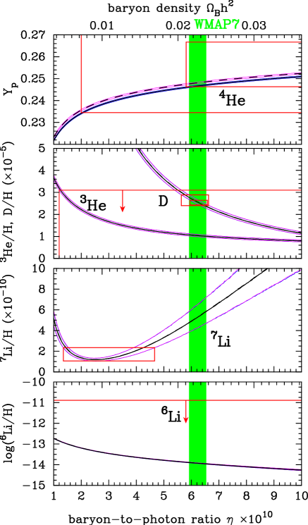
Figure 1 shows abundances of 4He (; mass fraction), D, 3He, 7Li and 6Li (H; by number relative to H) as a function of the baryon-to-photon ratio or the baryon energy density of the universe. The solid and dashed curves are the results for neutron lifetimes of s Serebrov:2004zf and s Nakamura:2010zzi , respectively. Thin solid curves show 95 % ranges determined from uncertainties in nuclear reaction rates. The boxes represent the adopted abundance constraints. The vertical stripe represents the 2 limits provided by WMAP Larson:2010gs . This corresponds to or .
II.2 effects of magnetic field
We include effects of PMF through the magnetic energy density (Appendix 1), thermodynamic variables of electron and positron and their time evolutions (Appendixes 2, 3). Estimations for initial values of electron chemical potential are changed from those in the case of no magnetic field (Appendix 4). Equations to solve are similar to those in Ref. Kernan:1995bz . However, equations which are solved in the consistent numerical calculation (see Appendix A) are more complicated.
Final values are different for different initial values with a fixed initial value. The final value, instead of the initial value, should then be fixed to the value determined from WMAP Larson:2010gs as pointed out but not done in deriving the limit on [eq. (4)] in Ref. Grasso:1996kk . In this study we fixed the final value. The effect of the magnetic field on weak reaction rates has been long since found to be negligible Grasso:1996kk ; Kernan:1995bz . It is, therefore, not included in this calculation.
III Result
Figure 2 shows light element abundances as a function of the magnetic field amplitude in units of the critical value, i.e., at temperature K, or absolute value at the present epoch of , i.e., . G is the critical magnetic field (above which quantized magnetic levels appear Grasso:2000wj ). The two parameters are related by KmG]. The solid and dashed curves correspond to results for two different neutron lifetimes, and the boxes represent adopted abundance constraints (see Sec. II.1).
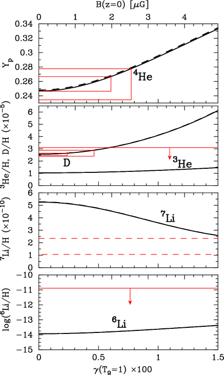
Figure 3 shows time evolutions of light element abundances as a function of the temperature . Solid lines correspond to the case of a magnetic field of G, while dashed lines correspond to SBBN.

The primordial abundance of 4He increases when the amplitude of PMF increases. The cosmic expansion rate is larger because of the energy of the PMF, so that the neutron abundance after the earlier freeze-out of weak reactions is higher. The time interval between the freeze-out and the 4He synthesis is also shorter because of faster cosmic expansion. Neutron abundances are larger than in SBBN for the above two reasons. Those neutrons are processed to form 4He nuclei. This is the reason of the trend of 4He abundance vs. value.
Because of the earlier freeze-out of the reaction 1H()2H at the 4He synthesis, the relic neutron abundance is higher than in SBBN. This higher neutron abundance affects abundances of other light nuclei complicatedly. The abundance of D which is produced via 1H()2H is somewhat higher when is higher. 3H is produced via 2H()3H and destroyed via 3H()4He. The enhanced D abundance simply leads to a higher 3H abundance by a higher production rate. 3He, on the other hand, is produced via 2H()3He and destroyed via 3He()3H. The somewhat higher D abundance leads to higher production rate while the higher neutron abundance leads to higher destruction rate. Resultingly, the 3He abundance is slightly higher than in SBBN.
6Li is produced via 4He()6Li and destroyed via 6Li)3He, and 7Li is produced via 4He()7Li and destroyed via 7Li()4He. The abundances of both nuclides are then higher since those of D and T are higher at higher values. 7Be is produced via 4He(3He)7Be and destroyed via 7Be)7Li. Slightly higher abundance of 3He and rather higher abundance of neutron results in net reduction of 7Be abundance with respect to that of SBBN.
The final 7Li abundance is the sum of those for 7Li and 7Be. 7Be nuclei convert to 7Li nuclei by an electron capture process. Since the abundance of 7Be is larger than that of 7Li in SBBN, an existence of PMF reduces the final 7Li abundance.
Shapes of curves in Fig. 2 are explained as above. Increases in abundances of 4He and (D+3He) have been obtained in the previous investigation Grasso:1996kk , and are consistent with our result.
The following constraints are derived from Fig. 2.
| (6) |
| (7) |
If one conservatively takes the constraint on 4He abundance by AOS10, the observation of D abundance provides the strongest upper limits on PMF. The conservative upper limit from the mean value of QSO D/H ratio Pettini:2012ph is G [], while that from the best D/H measurement Pettini:2012ph is G []. The latter limit is nearly identical to the previous estimation (corresponding to which is read from eq. (4) in Ref. Grasso:1996kk ), while the former is less stringent than the former by a factor of two. Previous constraints Grasso:1996kk ; Kernan:1995bz ; Cheng:1996yi ; Grasso:2000wj have been derived neglecting changes in evolution of baryon-to-photon ratio . In our work, this effect is consistently taken into account, and the final value is fixed to the WMAP estimation. The present result is, therefore, most precise. Other improvements are updates of nuclear reaction rates, observational constraints on primordial abundances, and baryon-to-photon ratio.
IV Discussion
The constraint derived in this study is related to the local field amplitude contributed from all wavelengths, and is not for that measured at any particular scale Kernan:1995bz . The present amplitude of cosmological averaged field, i.e, , (or the energy density of magnetic field) is defined Kernan:1995bz by
| (8) |
where is the redshift, is the Hubble volume, and is the position vector. The conservative constraint is then G.
Magnetic fields on some scales depend on the spatial structure of field. The root mean square (rms) amplitude on scale Grasso:2000wj is
| (9) |
where is the comoving coherence length, and is a parameter determined from statistical properties of the magnetic field Grasso:2000wj .
The present constraint can be compared with those from other measurements summarized in Refs Neronov:2009gh ; Neronov:1900zz . We note that the new constraint [Eq. (7)] can be the strongest for small correlation scales of pc. Direct constraints on magnetic field strength at smallest scales are derived from observations of Zeeman effect of HI, OH and CN in molecular clouds and HI diffuse clouds 2010ApJ…725..466C . The smallest upper limit on the radial component of magnetic field is G for an HI cloud seen in absorption against radio source 3C 348 (a usable data in Ref. Heiles2004 ). Heiles and Troland used data of Zeeman-splitting of the 21 cm line Heiles2004 , and estimated a median total field strength G for HI clouds with scales of typically – , taking account of probability distribution function of total field strength and a random orientation of fields with respect to the line of sight Heiles:2005xi .
The constraint on PMF from BBN studies cannot be directly compared with those from CMBR studies (e.g. Yamazaki:2004vq ; Yamazaki:2006bq ; Yamazaki:2008gr ; Yamazaki:2010nf ) , i.e., nG Yamazaki:2010nf , since the CMBR limits are imposed on magnetic fields on scales larger than the horizon in the BBN epoch. Grasso:2000wj . For example, when we adopt pc (the comoving Hubble horizon in the BBN epoch) and (which is derived in the assumption that a field vector performs a random walk in three dimensional space by steps of the physical scale 1983PhRvL..51.1488H ), Eq. (7) leads to
| (10) |
Comparisons between constraints for different coherent lengths thus generally depend on statistical properties of magnetic field. See Ref. Widrow:2011hs for a recent review for creation mechanisms of extragalactic magnetic fields and their problems.
V Conclusions
A new upper limit on the amplitude of primordial magnetic field (PMF) is derived by a comparison between a numerical calculation of elemental abundances in big bang nucleosynthesis and the latest constraints on abundances inferred from observations. The newest nuclear reaction rates are adopted (Sec. II). In addition, effects of PMF on the abundances are consistently taken into account in the numerical calculation with a formulation of physical variables in a magnetic field (Appendix A).
We find that the existence of PMF increases abundances of 3He and 6Li, and decreases that of 7Li in the calculation for the baryon-to-photon ratio determined from the measurement of cosmic microwave background radiation with the Wilkinson Microwave Anisotropy Probe. As a result of the rigorous calculation, we derive a constraint on the present amplitude of PMF, i.e., G [corresponding to the amplitude less than times the critical magnetic field strength for electron at temperature K].
Appendix A Formulae for effects of magnetic field on nucleosynthesis
-
1.
energy density
The energy density of magnetic field is
(11) where is the amplitude of magnetic field, and is the value in units of critical magnetic field, i.e., G with the electric charge, and the electron mass. This energy contributes to the total energy contents of the universe related to the Hubble expansion rate. In this study, it is assumed that the primordial magnetic field (PMF) just attenuates by the cosmic expansion.
-
2.
thermodynamic variables of electron in a magnetic field
The number density, energy density and the pressure 333The equation (2) of Ref. Grasso:1996kk was right, while the equation (2.15) of Ref. Cheng:1996yi was likely wrong. of the electron and positron are given Grasso:2000wj , respectively, as
(12) (13) (14) where
(15) is the Fermi-Dirac distribution function at electron temperature , and is the energy of electron in the presence of a uniform field which is much smaller than the critical strength Kernan:1995bz , and are the principal and magnetic quantum numbers of the Landau level, respectively, and is the chemical potential of electron. It has been assumed that the direction of field is the -axis.
The above quantities can be rewritten in the form of
(16) (17) (18) where , , , and were defined.
Using the Euler-McLaurin formula 444Kernan et al. Kernan:1995bz concluded that weak interaction rates decrease with increasing magnetic fields, while Cheng et al. Cheng:1996yi concluded that the rates increase with the fields. This contradiction was caused since the former authors used the Euler-McLaurin expansion, while the latter used the Taylor expansions of the rates which are ill defined Kernan:1996ab ., the number density and the energy density of electron and positron are given by
(19) (20) These equations are the same as those derived in Ref. Kernan:1995bz except that ours are generalized versions including the electron chemical potential. In order to follow in numerical calculations precisely the electron chemical potential, which becomes large at late time of BBN, it is kept in our formulation. Adopting the Euler-McLaurin formula to the pressure of electron and positron, one can obtain the equation, i.e.,
(21) Eqs. (19), (20) and (21) reproduce values for the case of no magnetic field when is input.
Time evolutions of following three variables as perturbations induced by a magnetic field are calculated. The first is related to the asymmetry in number abundances of electron and positron, i.e,
(22) where is the Planck’s constant, is the light speed, and
(23) and the parameter was defined. Partial derivatives of this function with respect to , the neutrino temperature, i.e, , and are given by
(24) (25) (26) where we used .
The second variable is a perturbation in the total energy density of electron and positron induced by , i.e.,
(27) where
(28) was defined. Partial derivatives of this function with respective to , and are given by
(29) (30) (31) The third variable is a perturbation in the total pressure of electron and positron, i.e.,
(32) where
(33) was defined.
-
3.
density–temperature relation
In the BBN code Kawano1992 , derivatives of with respect to , with the scale factor of the universe, and with the charge and the number ratio of nuclide to total baryon, respectively, are calculated and used. In the calculation, we use the following equation for charge conservation in the universe:
(34) where is the number density of in an environment of magnetic field , is the Avogadro’s number, and is the Boltzmann’s constant.
The left and right-hand sides are denoted as and , respectively. Taking derivatives of both sides with respect to , and , three partial derivatives are obtained as in the case of no magnetic field Kawano1992 :
(35) (37) where we used . The above derivatives are estimated utilizing Eqs. (22–26), and used in estimation of time evolution of the chemical potential parameter .
is given by
(38) where can be described as
(39) The conservation of energy for mixed matter of , ’s, and baryons leads Kawano1992 to
(40) where and are energy densities of photon and baryons, respectively, and and are pressures of photon and baryons, respectively.
Time derivative of the electron and positron energy density is given by
(41) Using Eqs. (40) and (41), we obtain
(42) The derivatives of [cf. Eqs. (27–31)] and pressure value [Eq. (32–33)] are input in this equation.
It is clear that a PMF enhances energy density of + [Eqs. (27) and (28)]. The PMF, however, does not work on , so that the enhanced energy of realizes by an energy transfer through interaction with thermal bath. When the temperature decreases, the energy gain of decreases because of the weakening of PMF. Resultingly, this loss of energy gain heats the thermal bath. This effect is taken into account in Eq. (42) 555Kernan, Starkman and Vachaspati Kernan:1995bz have suggested an error of Cheng et al. Cheng:1993kz that the PMF is included in the work-energy equation for photon..
-
4.
initial value of electron chemical potential
Using Eqs. (22), (34) and the fact of in hot environments before the nucleosynthesis, we obtain an equation for initial value of electron chemical potential, i.e.,
(43) where Kawano1992 was defined with the modified Bessel functions.
-
5.
note
Some transformations in equations are used in order to avoid appearances of divergences in a numerical calculation. They include , and .
Appendix B Effect on nuclear reaction rates
It was claimed that relatively weak magnetic fields reduce collision rates of nuclear reactions by a factor of two through alignments of directions in which charged nuclei can move 1986PPCF…28..857I ; 1987PPCF…29..951I . The claim is, however, wrong 1987PPCF…29..949J ; 1987PPCF…29..953H since it was based on a completely-mistaken treatment of 2D space perpendicular to the field direction, and cases of and are not treated consistently.
Precise reaction rates are derived below. The point is that a target is hit by projectiles coming from all directions although the distribution function of projectile charged particles are quantized.
B.1 Nuclear distribution function
Magnetic fields would affect nuclear reaction rates through a discretization of momentum on the plane perpendicular to the field direction (-axis). The Zeeman splitting also realizes in magnetic fields. It is, however, neglected in this study since situations of large fields are eventually excluded from light element abundances deviated through their effects on the cosmic expansion rate. Energy levels of charged nuclides are then given by
| (44) |
where and are the mass and the charge number of a nuclide, respectively.
The nuclear distribution function is discretized similarly to the case of electron as
| (45) |
where is the statistical weight, and is the chemical potential of the nuclide. The number density of nuclide in a Landau level and in a momentum range between and is given by
| (46) |
The total number density is given by
| (47) | |||||
where
| (48) |
was defined.
B.2 Rates of reactions between charged particles
The thermal average of reaction rate is described as
| (50) |
where is the relative velocity of nuclides 1 and 2, is the kinetic energy in the center of mass (CM) system, and is the angle between momentum vectors of nuclides 1 and 2 on the plane perpendicular to the magnetic field.
The velocity vectors of nuclides is described as . The angle is then given by with amplitudes of the vectors . The relative velocity is given by with . The CM kinetic energy is with the reduced mass .
Substituting Eq. (49) in Eq. (50), we obtain an equation,
| (51) | |||||
Momentum variables, i.e., and , are transformed to the CM momentum and the relative momentum. Integration over the CM momentum is performed in the equation, and we obtain,
where is the relative velocity in the direction of the field.
Velocities on the plane perpendicular to the field are discretized as . The relative velocity can then be described by
| (53) |
B.3 Rates of reactions between a neutron and charged particles
In reactions of neutron, discrete momenta of only charged particles are taken into account. The rate is described as
| (54) |
Variable transformations from and to (CM momentum) and (relative momentum) are performed, and an integration over is computed. The reaction rate is then rewritten to be
| (55) | |||||
We perform an integration over azimuth angle on the () plane and trivial transformations from momenta to velocities, and obtain an expression, i.e.,
| (56) | |||||
where the relative velocity is given by
| (57) |
The kinetic energy in the CM system is given by .
The sum in the reaction rate is transformed to an integration using the Euler-McLaurin formula. The integration form of reaction rate is given by
| (58) | |||||
Two terms scaling as are induced by magnetic field , and they disappear in the limit of no field, i.e., .
B.3.1 7Be()7Li
We check the reaction rate of 7Be()7Li for example. Rates are calculated with Eq. (56). The masses of neutron and 7Be nucleus is GeV and GeV Audi2003 . Although the cross section would be changed in magnetic fields through the momentum quantization, that effect is neglected and cross section values in no fields are taken from Ref. Descouvemont2004 approximately.
Figure 4 shows calculated rates of 7Be()7Li as a function of . Solid dark lines correspond to cases in which magnetic fields decrease with time because of the cosmic expansion as . Field amplitudes are , and , in order of increasing line width (from the top to the bottom), respectively. Dashed lines, on the other hand, correspond to cases of constant magnetic field of , and , in order of increasing line width (from the top to the bottom), respectively. Solid gray line corresponds to the rate in no magnetic field. The uppermost solid and dashed lines are hardly distinguishable from the solid gray line.
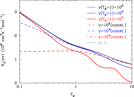
In the attenuating magnetic field case (solid dark lines), the field effect is larger in higher temperatures. The discretization effect is roughly determined from the index factor, i.e., , in the exponential in Eq. (56). The field amplitude () decreases faster than the temperature in the universe () does. The index is, therefore, larger in higher temperature. In the constant magnetic field case (dashed lines), the field effect is larger in lower temperatures conversely.
In somewhat high magnetic field, the minimum energy of nuclear Landau level is higher than the thermal energy of the universe, . The average of rate then receives a contribution from large CM energies which originate from large relative velocities [Eq. (57)]. Since the reaction rate at higher energies is roughly smaller as for the reaction 7Be()7Li, the existence of field decreases the reaction rate. The lowest solid dark line in Fig. 4 has two bumps at and . These bumps correspond to peaks in reaction rates produced by the resonant states of 9Be∗ at resonance energies MeV and MeV Adahchour2003 . At and , the minimum CM energies of the ground Landau level, i.e., [cf. Eq. (57)], are MeV and MeV, respectively.
As observed above, magnetic fields can affect thermonuclear reaction rates. Large amplitudes of magnetic fields as assumed in Fig. 4 are, however, excluded from incredibly fast expansion of universe (see Fig. 2). The effect of magnetic field on nuclear reaction rates can thus be neglected.
Acknowledgements.
This work is supported by Grant-in-Aid for Scientific Research from the Ministry of Education, Science, Sports, and Culture (MEXT), Japan, No.22540267 and No.21111006 (Kawasaki) and JSPS Grant No.21.6817 (Kusakabe) and by World Premier International Research Center Initiative (WPI Initiative), MEXT, Japan.References
- (1) G. Gamow, Phys. Rev. 70, 572 (1946)
- (2) R. A. Alpher, H. Bethe, and G. Gamow, Phys. Rev. 73, 803 (1948)
- (3) R. A. Alpher and R. C. Herman, Phys. Rev. 74, 1737 (1948)
- (4) C. Hayashi, Progress of Theoretical Physics 5, 224 (1950)
- (5) R. A. Alpher, J. W. Follin, and R. C. Herman, Phys. Rev. 92, 1347 (1953)
- (6) R. V. Wagoner, W. A. Fowler, and F. Hoyle, Astrophys. J. 148, 3 (1967)
- (7) C. Hayashi and M. Nishida, Progress of Theoretical Physics 16, 613 (1956)
- (8) H. Sato, Progress of Theoretical Physics 38, 1083 (1967)
- (9) R. A. Alpher and R. C. Herman, Phys. Rev. 75, 1089 (1949)
- (10) A. A. Penzias and R. W. Wilson, Astrophys. J. 142, 419 (1965)
- (11) W. A. Fowler, G. R. Caughlan, and B. A. Zimmerman, Annu. Rev. Astron. Astrophys. 5, 525 (1967)
- (12) R. V. Wagoner, Astrophys. J. 179, 343 (1973)
- (13) K. A. Olive, D. N. Schramm, G. Steigman, M. S. Turner, and J.-M. Yang, Astrophys J. 246, 557 (1981)
- (14) D. A. Dicus, E. W. Kolb, A. M. Gleeson, E. C. G. Sudarshan, V. L. Teplitz, and M. S. Turner, Phys. Rev. D 26, 2694 (1982)
- (15) J. Audouze, D. Lindley, and J. Silk, Astrophys. J. 293, L53 (1985)
- (16) A. M. Boesgaard and G. Steigman, Ann. Rev. Astron. Astrophys. 23, 319 (1985)
- (17) K. A. Olive, D. N. Schramm, G. Steigman, and T. P. Walker, Phys. Lett. B236, 454 (1990)
- (18) L. M. Krauss and P. Romanelli, Astrophys. J. 358, 47 (1990)
- (19) M. S. Smith, L. H. Kawano, and R. A. Malaney, Astrophys. J. Suppl. 85, 219 (1993)
- (20) R. A. Malaney and G. J. Mathews, Phys. Rept. 229, 145 (1993)
- (21) C. J. Copi, D. N. Schramm, and M. S. Turner, Science 267, 192 (1995)
- (22) L. M. Krauss and P. J. Kernan, Phys. Lett. B347, 347 (1995)
- (23) S. Sarkar, Rept. Prog. Phys. 59, 1493 (1996)
- (24) K. A. Olive and S. T. Scully, Int. J. Mod. Phys. A11, 409 (1996)
- (25) N. Hata et al., Phys. Rev. Lett. 75, 3977 (1995)
- (26) B. D. Fields, K. Kainulainen, K. A. Olive, and D. Thomas, New Astron. 1, 77 (1996)
- (27) D. N. Schramm and M. S. Turner, Rev. Mod. Phys. 70, 303 (1998)
- (28) S. Esposito, G. Mangano, G. Miele, and O. Pisanti, Nucl. Phys. B568, 421 (2000)
- (29) S. Burles, K. M. Nollett, J. W. Truran, and M. S. Turner, Phys. Rev. Lett. 82, 4176 (1999)
- (30) D. Tytler, J. M. O’Meara, N. Suzuki, and D. Lubin, Physica Scripta Volume T 85, 12 (2000)
- (31) E. Vangioni-Flam, A. Coc, and M. Casse, Astron. Astrophys. 360, 15 (2000)
- (32) S. Burles, K. M. Nollett, and M. S. Turner, Astrophys. J. 552, L1 (2001)
- (33) R. H. Cyburt, B. D. Fields, and K. A. Olive, New Astron. 6, 215 (2001)
- (34) A. Coc, E. Vangioni-Flam, M. Casse, and M. Rabiet, Phys. Rev. D65, 043510 (2002)
- (35) A. Coc, E. Vangioni-Flam, P. Descouvemont, A. Adahchour, and C. Angulo, Astrophys. J. 600, 544 (2004)
- (36) F. Iocco, G. Mangano, G. Miele, O. Pisanti, and P. D. Serpico, Phys. Rept. 472, 1 (2009)
- (37) G. Mangano and P. D. Serpico, Phys. Lett. B701, 296 (2011)
- (38) A. Coc, S. Goriely, Y. Xu, M. Saimpert, and E. Vangioni, Astrophys.J. 744, 158 (2012)
- (39) D. N. Spergel et al. (WMAP), Astrophys. J. Suppl. 148, 175 (2003)
- (40) D. N. Spergel et al. (WMAP), Astrophys. J. Suppl. 170, 377 (2007)
- (41) D. Larson et al., Astrophys. J. Suppl. 192, 16 (2011)
- (42) R. H. Cyburt, B. D. Fields, and K. A. Olive, JCAP 0811, 012 (2008)
- (43) M. Kawasaki and M. Kusakabe, Phys. Rev. D83, 055011 (2011)
- (44) R. F. O’Connell and J. J. Matese, Nature (London) 222, 649 (1969)
- (45) G. Greenstein, Nature (London) 223, 938 (1969)
- (46) J. J. Matese and R. F. O’Connell, Astrophys. J. 160, 451 (1970)
- (47) B.-l. Cheng, D. N. Schramm, and J. W. Truran, Phys. Rev. D49, 5006 (1994)
- (48) D. Grasso and H. R. Rubinstein, Astropart. Phys. 3, 95 (1995)
- (49) P. J. Kernan, G. D. Starkman, and T. Vachaspati, Phys. Rev. D54, 7207 (1996)
- (50) D. Grasso and H. R. Rubinstein, Phys. Lett. B379, 73 (1996)
- (51) B.-l. Cheng, A. V. Olinto, D. N. Schramm, and J. W. Truran, Phys. Rev. D54, 4714 (1996)
- (52) P. J. Kernan, G. D. Starkman, and T. Vachaspati, Phys. Rev. D56, 3766 (1997)
- (53) I.-S. Suh and G. J. Mathews, Phys. Rev. D59, 123002 (1999)
- (54) D. Grasso and H. R. Rubinstein, Phys. Rept. 348, 163 (2001)
- (55) E. Aver, K. A. Olive, and E. D. Skillman, JCAP 1005, 003 (2010)
- (56) L. Kawano, NASA STI/Recon Technical Report N 92, 25163 (1992)
- (57) R. H. Cyburt et al., Astrophys. J. Suppl. Ser. 189, 240 (2010)
- (58) A. Serebrov et al., Phys. Lett. B605, 72 (2005)
- (59) K. Nakamura et al. (Particle Data Group), J. Phys. G37, 075021 (2010)
- (60) S. Ando, R. H. Cyburt, S. W. Hong, and C. H. Hyun, Phys. Rev. C74, 025809 (2006)
- (61) P. Descouvemont, A. Adahchour, C. Angulo, A. Coc, and E. Vangioni-Flam, Atomic Data and Nuclear Data Tables 88, 203 (2004)
- (62) R. H. Cyburt and B. Davids, Phys. Rev. C78, 064614 (2008)
- (63) A. P. Serebrov and A. K. Fomin, Phys. Rev. C82, 035501 (2010)
- (64) G. J. Mathews, T. Kajino, and T. Shima, Phys. Rev. D71, 021302 (2005)
- (65) M.-K. Cheoun, T. Kajino, M. Kusakabe, and G. J. Mathews, Phys. Rev. D84, 043001 (2011)
- (66) This value is close to an average lifetime of s estimated Serebrov:2011re by including recent yet unpublished reports of experiments with ultracold neutrons (see their references)
- (67) M. Pettini and R. Cooke(2012), arXiv:1205.3785 [astro-ph.CO]
- (68) T. M. Bania, R. T. Rood, and D. S. Balser, Nature 415, 54 (2002)
- (69) Y. I. Izotov and T. X. Thuan, Astrophys. J. 710, L67 (2010)
- (70) L. Sbordone et al., Astron. Astrophys. 522, A26 (2010)
- (71) M. Steffen, R. Cayrel, P. Bonifacio, H.-G. Ludwig, and E. Caffau, in IAU Symposium, IAU Symposium, Vol. 265, edited by K. Cunha, M. Spite, & B. Barbuy (2010) pp. 23–26
- (72) M. Asplund, D. L. Lambert, P. E. Nissen, F. Primas, and V. V. Smith, Astrophys. J. 644, 229 (2006)
- (73) A. Neronov and D. V. Semikoz, Phys. Rev. D80, 123012 (2009)
- (74) A. Neronov and I. Vovk, Science 328, 73 (2010)
- (75) R. M. Crutcher, B. Wandelt, C. Heiles, E. Falgarone, and T. H. Troland, Astrophys. J. 725, 466 (2010)
- (76) C. Heiles and T. H. Troland, Astrophys. J. Suppl. Ser. 151, 271 (2004)
- (77) C. Heiles and T. Troland, Astrophys.J. 624, 773 (2005)
- (78) D. G. Yamazaki, K. Ichiki, and T. Kajino, Astrophys. J. 625, L1 (2005)
- (79) D. Yamazaki, K. Ichiki, T. Kajino, and G. J. Mathews, Astrophys. J. 646, 719 (2006)
- (80) D. G. Yamazaki, K. Ichiki, T. Kajino, and G. J. Mathews, Phys. Rev. D77, 043005 (2008)
- (81) D. G. Yamazaki, K. Ichiki, T. Kajino, and G. J. Mathews, Phys. Rev. D81, 023008 (2010)
- (82) C. J. Hogan, Physical Review Letters 51, 1488 (1983)
- (83) L. M. Widrow et al., Space Sci. Rev., 300(2011)
- (84) The equation (2) of Ref. Grasso:1996kk was right, while the equation (2.15) of Ref. Cheng:1996yi was likely wrong.
- (85) Kernan et al. Kernan:1995bz concluded that weak interaction rates decrease with increasing magnetic fields, while Cheng et al. Cheng:1996yi concluded that the rates increase with the fields. This contradiction was caused since the former authors used the Euler-McLaurin expansion, while the latter used the Taylor expansions of the rates which are ill defined Kernan:1996ab .
- (86) Kernan, Starkman and Vachaspati Kernan:1995bz have suggested an error of Cheng et al. Cheng:1993kz that the PMF is included in the work-energy equation for photon.
- (87) S. Imazu, Plasma Physics and Controlled Fusion 28, 857 (1986)
- (88) S. Imazu, Plasma Physics and Controlled Fusion 29, 951 (1987)
- (89) O. N. Jarvis, Plasma Physics and Controlled Fusion 29, 949 (1987)
- (90) M. G. Haines, Plasma Physics and Controlled Fusion 29, 953 (1987)
- (91) G. Audi, A. H. Wapstra, and C. Thibault, Nuclear Physics A 729, 337 (2003)
- (92) A. Adahchour and P. Descouvemont, Journal of Physics G Nuclear Physics 29, 395 (2003)
- (93) A. P. Serebrov and A. K. Fomin(2011), arXiv:1104.4238 [nucl-ex]