Phase structures in fuzzy geometries

Abstract:

We study phase structures of quantum field theories in fuzzy geometries. Several examples of fuzzy geometries as well as QFT’s on such geometries are considered. They are fuzzy spheres and beyond as well as noncommutative deformations of BTZ blackholes. Analysis is done analytically and through simulations. Several features like novel stripe phases as well as spontaneous symmetry breaking avoiding Colemen, Mermin, Wagner theorem are brought out. Also we establish that these phases are stable due to topological obstructions.

1 Introduction

General relativity and quantum mechanics together imply that space-time structure at the Planck scale is not described by conventional notions of geometry. This was pointed out by many. In particular see Doplicher etal., [1] as well as Werner Nahm (see [2]). These come about due to appearance of null horizons. Interestingly extra dimensional spacetimes with higher dimensional ‘Planck scale’ $\displaystyle O(Tev)$ will require the extra dimensional space description to be fuzzy. Surprisingly the difficulties in defining geometry at infinitesimal distances were anticipated much earliar: ‘it seems that empirical notions on which the metrical determinations of space are founded, the notion of a solid body and a ray of light cease to be valid for the infinitely small. We are therefore quite at liberty to suppose that the metric relations of space in the infinitely small do not conform to hypotheses of geometry; and we ought in fact to suppose it, if we can thereby obtain a simpler explanation of phenomena’: Riemann, [3]

Field theories on non-commutative geometries are inherently non-local leading to mixing of the infrared and ultraviolet scales. This, in turn, is responsible for new ground states with spatially varying condensates. Many non-perturbative studies have established that non-commutative spaces, such as the Groenewold-Moyal plane and fuzzy spheres, allow for the formation of stable non-uniform condensates as ground states. Exploring such implications of the non-local nature of field theories is very important in many areas of quantum physics. [4, 5]

Since different phases are intimately connected with spontaneous symmetry breaking (SSB), the role of symmetries in noncommutative geometries themselves is subtle. This issue is important in 2D because the Coleman-Mermin-Wagner (CMW) theorem states that there can be no SSB of continuous symmetry on 2-dimensional commutative spaces. There is no obvious generalisation of the CMW theorem for non-commutative spaces, since the theorem relies strongly on the locality of interactions. Non-commutative spaces admit non-uniform solutions (in the mean field) and one can ask the question what happens to the stability of these configurations. Non-uniform condensates naturally have an infra-red cut-off for the fluctuations. This cut-off softens the otherwise divergent contributions of the Goldstone modes[6, 7, 10, 11, 8, 13, 9, 14].

There have been various attempts to study gravity theories within the noncommutative framework [15, 16]. This has led to a Hopf algebraic description of noncommutative black holes [17, 18] and FRW cosmologies [19]. A large class of such black hole solutions, including the noncommutative BTZ [20, 21] and Kerr black holes, exhibits an universal feature where the Hopf algebra is described by a noncommutative cylinder [22], which belongs to the general class of the $\displaystyle\kappa$-Minkowski algebras [23, 24, 25, 26]. we shall take the noncommutative cylinder and the associated algebra as a model for noncommutative black holes.

The study of quantum field theories in the background of black holes has led to the discovery of interesting features associated with the underlying geometry, such as the Hawking radiation and black hole entropy. In the noncommutative case, the black hole geometry is replaced with the algebra defined by the noncommutative cylinder. In order to probe the features of a noncommutative black hole, it is useful to analyze the behaviour of a quantum fields coupled to the noncommutative cylinder algebra. Scalar field theories have been extensively studied on $\displaystyle\kappa$-Minkowski spaces [27, 28, 29, 30, 32], which has led to twisted statistics and deformed oscillator algebra for the quantum field [29, 30, 31]. Theories on the noncommutative cylinder lead to quantization of the time operator [33, 34]. See Madore [35] or Balachandran et al [36] for an introduction to fuzzy geometries.

In this paper we discuss examples of fuzzy geometries in Sec 2. In Sec 3 we consider QFT’s on such geometries. Following this in Sec 4 we take up aspects of numerical simulations of flutuations of fields on fuzzy geometries and present our results. Lastly we conclude with discussions on implications of our results in Sec 5.

2 Examples of fuzzy geometry

It has been well known that representations of $\displaystyle SU(2)$ Lie-algebra provide a basis for the study of functions on a fuzzy spheres. This can be understood by the quantisation of coadjoint orbits $\displaystyle{SU(2)}/{U(1)}$. The generators of the Lie algebra $\displaystyle X_{i}$ satisfy:

$$[X_{i},X_{j}]~{}=~{}i\epsilon_{ijk}X_{k},\qquad\sum X_{i}^{2}~{}=~{}R^{2}.$$ (1)

The fact $\displaystyle S^{2}~{}=~{}CP^{1}$ is a coadjoint orbit is useful in quantising this space. This can be extended to $\displaystyle CP^{2}~{}=~{}{SU(3)}/{SU(2)\otimes U(1)}$ and any $\displaystyle CP^{n}$. The fuzzy torus is defined by the two generators $\displaystyle U,V$ satisfying $\displaystyle U~{}V~{}=~{}e^{i\theta}~{}V~{}U$. Finite dimensional representations can easily be constructed for this algebra for rational $\displaystyle\theta$. We will explain certain non standard ones.

2.1 Higgs algebra

The Higgs algebra is defined by $\displaystyle[X_{+},X_{-}]~{}=~{}\alpha Z+\beta Z^{3},~{}[X_{\pm},Z]~{}=~{}\mp X_{+}$. It can be easily checked that the Casimir for this algebra is given by:

$$\mathcal{C}=\frac{1}{2}\left[\{X_{+},X_{-}\}+g(Z)+g(Z-1)\right],$$ (2)

where $\displaystyle g(Z)$ is

$$g(Z)=C_{0}+\frac{\alpha}{2}\,Z(Z+1)+\frac{\beta}{4}\,Z^{2}(Z+1)^{2}.$$ (3)

For $\displaystyle C_{0}=\mu^{2}$, $\displaystyle\alpha=-2(2\mu~{}+~{}1)$, and $\displaystyle\beta=4$ The Casimir reduces to the expression: $\displaystyle X^{2}+Y^{2}+(Z^{2}~{}-~{}\mu)^{2}$. Equating the Casimir to 1 and plotting the function for different values of $\displaystyle\mu$ we see interesting topology change [37].

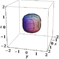
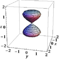
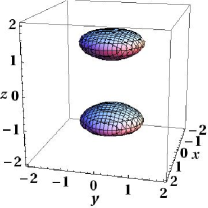
Figure 1: Surface plots depicting the change in topology for $\displaystyle\mu=0,1,1/2$.

Such changes in the topology were first considered by Arnlind etal [38].

2.2 Fuzzy cylinder

The NC cylinder is defined by the relation

$$\left[~{}Z,~{}e^{i\phi}~{}\right]~{}=~{}\alpha e^{i\phi}$$ (4)

where $\displaystyle Z$ is hermitian and $\displaystyle e^{i\phi}$ is unitary. Since we are interested in simulations, we have to discretise the above NC cylinder.

In the rest of this paper, we will work with $\displaystyle\alpha=1$ without loss of generality, since the simple scaling $\displaystyle Z\rightarrow Z/\alpha$ can scale $\displaystyle\alpha$ away in the commutation relation (4).

For this purpose consider the spin $\displaystyle J$ irreducible representation (IRR) of the $\displaystyle SU(2)$ Lie algebra, given by

$$[X_{+},X_{-}]~{}=~{}2X_{3},~{}~{}[X_{\pm},X_{3}]~{}=~{}\mp X_{\pm}.$$ (5)

Since the operator $\displaystyle Z$ generates rotations around the axis of the cylinder, it can be identified with $\displaystyle X_{3}$. But when we use the finite dimensional representations of $\displaystyle SU(2)$ we cannot implement (4) with unitarity for $\displaystyle e^{i\phi}$. For this purpose, we decompose $\displaystyle X_{+}$ as product of a unitary and a Hermitian operator as given by

$$X_{+}~{}=~{}e^{i\phi}~{}R$$ (6)

Here $\displaystyle R$ is necessarily singular and can not be inverted. However a partial inverse $\displaystyle\tilde{R}$ can be found such that $\displaystyle R\tilde{R}~{}=~{}P$, the projector such that $\displaystyle 1-P$ projects to the kernel of $\displaystyle R$. Thus we get

$$~{}[Z,e^{i\phi}]~{}P=~{}e^{i\phi}~{}P$$ (7)

To find a representation for $\displaystyle R$ and $\displaystyle e^{i\phi}$, we can look at

$$\displaystyle R^{2}=X_{-}X_{+}=\vec{L}^{2}-L_{3}(L_{3}+1)$$ (8)

which commutes with $\displaystyle Z=L_{3}$. Remember that in the usual representation of angular momentum, $\displaystyle L_{3}|l,m>=m|l,m>$ with $\displaystyle|m|\leq l$. Shifting the indices from $\displaystyle 0$ to $\displaystyle 2l+1=2J$, we have $\displaystyle j=m+l+1$, leading to

$$\displaystyle X_{-}X_{+}|l,m> \displaystyle= \displaystyle[l(l+1)-m(m+1)]|l,m>=[(l+1/2)^{2}-(m+1/2)^{2}]|l,m>$$

$$\displaystyle X_{-}X_{+}|J,j> \displaystyle= \displaystyle[J^{2}-(J-j)^{2}]|J,j>=j(2J-j)|J,j>$$

There is only one hermitian positive solution to this equation which takes the form

$$R_{ij}~{}=~{}\sqrt{i(2J-i)}~{}\delta_{i,j}$$ (9)

which is diagonal as expected, and whose null space is along the top state $\displaystyle|J,2J>$. As a result, $\displaystyle P=1-|J,2J><J,2J|$, and

$$\tilde{R}=\sum_{i=1}^{2J-1}[i(2J-i)]^{-1/2}\,|J,i><J,i|$$

where the sum stops at $\displaystyle i=2J-1$ so that there is a zero in the last position on the diagonal. It is now possible to deduce the first $\displaystyle 2J-1$ lines of the unitary matrix $\displaystyle e^{i\phi}$ from (6):

$$\left.\begin{array}[]{rcl}X_{+}|J,j>&=&\sqrt{j(2J-j)}|J,j+1>\\ X_{+}|J,j>&=&e^{i\phi}~{}R|J,j>=\sqrt{j(2J-j)}e^{i\phi}~{}|J,j>\end{array}\right\}\Rightarrow e^{i\phi}~{}|J,j>=|J,j+1>,\ j<2J.$$

Eq. (6) yields no equation for the last column which is instead determined from its unitarity. The columns $\displaystyle 1,\cdots,2J-1$ of $\displaystyle e^{i\phi}$, given by $\displaystyle|J,j+1>$, form an orthonormal set, as expected for a unitary matrix. Then the last column will be a vector orthogonal to all these vectors and thus can only be proportional to $\displaystyle|J,1>$. After normalisation that still leaves a $\displaystyle U(1)$ freedom so that

$$(e^{i\phi})_{ij}~{}=~{}\delta_{i,j+1}~{}+~{}e^{i\beta}~{}\delta_{i,1}\delta_{j,2J}$$ (10)

where $\displaystyle\beta$ can be any real number. For $\displaystyle\beta=0$, $\displaystyle e^{i\phi}$ is just a circular permutation of length $\displaystyle 2J$.

2.3 Noncommutative BTZ blackhole

We briefly summarize the essential features of a noncommutative black hole which is useful for our analysis. In the commutative case, a non-extremal BTZ black hole is described in terms of the coordinates $\displaystyle(r,\phi,t)$ and is given by the metric [20, 21]

$$ds^{2}=\biggl{(}M-\frac{r^{2}}{\ell^{2}}-\frac{J^{2}}{4r^{2}}\biggr{)}dt^{2}-\biggl{(}M-\frac{r^{2}}{\ell^{2}}-\frac{J^{2}}{4r^{2}}\biggr{)}^{-1}dr^{2}+r^{2}\biggl{(}d\phi-\frac{J}{2r^{2}}dt\biggr{)}^{2}\;,$$ (11)

where $\displaystyle 0\leq r<\infty\;,\;-\infty<t<\infty\;,\;0\leq\phi<2\pi\;,$ $\displaystyle M$ and $\displaystyle J$ are respectively the mass and spin of the black hole, and $\displaystyle\Lambda=-1/\ell^{2}$ is the cosmological constant. In the non-extremal case, the two distinct horizons $\displaystyle r_{\pm}$ are given by

$$r_{\pm}^{2}=\frac{M\ell^{2}}{2}\biggl{\{}1\pm\bigg{[}1-\biggl{(}\frac{J}{M\ell}\biggr{)}^{2}\biggr{]}^{\frac{1}{2}}\biggr{\}}.\;$$ (12)

An alternative way to obtain the geometry of the BTZ black hole is to quotient the manifold $\displaystyle AdS_{3}$ or $\displaystyle SL(2,R)$ by a discrete subgroup of its isometry. The noncommutative BTZ black hole is then obtained by a deformation of $\displaystyle AdS_{3}$ or $\displaystyle SL(2,R)$ which respects the quotienting [17]. In the noncommutative theory, the coordinates $\displaystyle r$, $\displaystyle\phi$ and $\displaystyle t$ are replaced by the corresponding operators $\displaystyle\hat{r}$, $\displaystyle\hat{\phi}$ and $\displaystyle Z$ respectively, that satisfy the algebra

$$[\hat{t},e^{i\hat{\phi}}]=\alpha e^{i\hat{\phi}}\qquad[\hat{r},\hat{t}]=[\hat{r},e^{i\hat{\phi}}]=0\;,$$ (13)

where the constant $\displaystyle\alpha$ is proportional to $\displaystyle\ell^{3}/(r_{+}^{2}-r_{-}^{2})$. We shall henceforth refer to (13) as the noncommutative cylinder algebra. Furthermore, $\displaystyle\hat{t}$ denoting the operator corresponding the the axis of the cylinder, it will be therefore identified as the operator $\displaystyle Z$ in the following sections.

It may be noted that the operator $\displaystyle\hat{r}$ is in the center of the algebra (13). In addition, it can be shown easily that $\displaystyle e^{-2\pi i\hat{t}/\alpha}$ belongs to the center of (13) as well. Hence, in any irreducible representation of (13), the element $\displaystyle e^{-2\pi i\hat{t}/\alpha}$ is proportional to the identity,

$$e^{-2\pi i\hat{t}/\alpha}=e^{i\gamma}{\rm 1\!l},$$ (14)

where $\displaystyle\gamma\in R$ mod $\displaystyle(2\pi)$. Eqn. (14) implies that in any irreducible representation of (13), the spectrum of the time operator $\displaystyle\hat{t}$, or $\displaystyle Z$, is quantized [22, 33, 34] and is given by

$${\rm{spec}}~{}{\hat{t}}=n\alpha-\frac{\gamma\alpha}{2\pi}\;,\;\;n\in{\mathbb{Z}}.$$ (15)

In what follows we shall set $\displaystyle\gamma=0$ without loss of generality.

The noncommutative cylinder algebra (13) belongs to a special class of $\displaystyle\kappa$ - Minkowski algebra and it appears in the description of noncommutative Kerr black holes [18] and FRW cosmologies [19]. We shall henceforth consider (13) as a prototype of the noncommutative black hole.

3 Scalar fields on fuzzy spheres/cylinder

We shall now present our analytic and numerical analysis of scalar fields on different fuzzy geometries.

Let $\displaystyle\Phi$ be a scalar field on a fuzzy sphere defined by spin $\displaystyle j~{}=~{}{(N-1)}/{2}$ representation. It is given by a $\displaystyle N\times N$ matrix. We consider the action given by:

$$S~{}=~{}\frac{4\pi}{N}~{}Tr~{}\{\Phi[L_{i}[L_{i},\Phi]\}~{}+~{}R^{2}\{r\Phi^{2}~{}+~{}\lambda\Phi^{4}~{}\}$$ (16)

It is easy to see the ground states are characterised by

$$\Phi=0,~{}~{}and\qquad\Phi\neq 0,~{}~{}but~{}~{}Tr~{}\Phi~{}=~{}0$$ (17)

which corresepond to the uniform and nonuniform or stripe phases. We can obtain the continuum limit by taking $\displaystyle N\longrightarrow\infty$. The planar limit is obtained by taking $\displaystyle R\longrightarrow\infty$. One gets commutative planar or noncommutative planar (Moyal) limit depending on $\displaystyle{R^{2}}/{N}\longrightarrow\infty$ or finite. If we have a complex scalar field $\displaystyle\Phi$ then global $\displaystyle U(1)$ symmetry can be broken contrary to the expectation from Coleman-Mermin-Wagner theorem in the NC limit. This is due to the nonlocality of NC geometries. This has been shown through simulations in [11].

3.1 Topological aspects on fuzzy spheres

But our interest in this work is to consider the topological aspects of nonlinear fields on fuzzy geometries. For this, we consider three hermitian scalar fields $\displaystyle\Phi_{i}$ with global $\displaystyle O(3)$ symmetry. The most general action upto quartic interactions takes the form,

$$S(\Phi)=\frac{4\pi}{N}\,{\rm Tr}\left[\sum_{i}|\left[L_{i},\Phi\right]|^{2}+R^{2}\left(r|\Phi|^{2}+i\beta\epsilon_{ijk}\Phi_{i}\Phi_{j}\Phi_{k}+\lambda(|\Phi|^{2})^{2}+\mu|\left[\Phi_{i},\Phi_{j}\right]|^{2}\right)\right]$$ (18)

In the mean-field the above theory admits a uniform condensate for $\displaystyle r<0$. However the fluctuations of the Goldstone mode render this solution unstable. Apart from the uniform condensate the above model admits many meta-stable solutions. To simplify our arguments we consider the case $\displaystyle\beta~{}=~{}0,\mu~{}=~{}0$: We are interested on those solutions which are stable due to topological obstructions. For example,

$$\Phi_{i}=~{}\alpha~{}L_{i},~{}~{}\rm{with}~{}~{}\alpha=\sqrt{\frac{\frac{2|r|}{\lambda}}{N^{2}-1}}$$ (19)

The analog of this configuration in continuum space is the hedgehog configuration where the $\displaystyle O(3)$ spin vector on the sphere is pointing radially outward. The spin is parallel to the position vector on the sphere. This configuration is topologically stable as it cannot be smoothly deformed to a uniform one. Similarly the above configuration cannot be smoothly deformed to $\displaystyle\Phi~{}=~{}I$ which is also a solution. The above configuration corresponds to a winding number one map from the physical space $\displaystyle S_{F}^{2}$ to the vacuum manifold which is also $\displaystyle S_{F}^{2}$. All topologically stable configurations in the continuum limit, can be characterised by the second homotopy group $\displaystyle\Pi_{2}(S^{2})$. For a discussion on topological classification of the maps $\displaystyle S_{F}^{2}\longrightarrow S_{F}^{2}$ see [12]. To study the net effect of topological nature of the background configuration and non-locality on fluctuations, we consider only the winding number one configuration which is given in Eq.(19). As mentioned our plan is to compute these fluctuations numerically. Even before computing the fluctuations one can make some general remarks about the behaviour of the fluctuations [11]. The effect of nonlocality basically provides a non-zero mass $\displaystyle O({\alpha}/{N})$ to the Goldstone mode fluctuations. This puts an infrared cut-off for the fluctutations. From our previous study [11] it seems that this mass/cutoff is mode dependent, as only higher modes of the condensate survived the fluctuations. As we will see from our results the combined effect of topology and nonlocality, the infrared cut-off drastically reduce the contribution of the fluctuations. Before presenting details of numerics let us also consider scalar field on fuzzy cylinder.

3.2 The Action on the fuzzy cylinder

Define $\displaystyle\widetilde{Tr}O~{}=~{}Tr(POP)$ where $\displaystyle P$ is the projection operator defined in [Eq: No] This trace $\displaystyle\widetilde{Tr}$ is equivalent to integrating over the whole cylinder in the continuum limit. We also need the derivatives $\displaystyle\partial_{\phi}$ and $\displaystyle\partial_{Z}$. They are:

$$\displaystyle\partial_{\phi}\Phi~{} \displaystyle= \displaystyle~{}[Z,\Phi]$$ (20)

$$\displaystyle\partial_{Z}\Phi~{} \displaystyle= \displaystyle~{}e^{-i\phi}[e^{i\phi},\Phi]$$ (21)

Then, apart from $\displaystyle J$-dependent normalisation factors, the action can be chosen as:

$$S~{}=~{}\widetilde{Tr}\left(|~{}[Z,\Phi]~{}|^{2}~{}+~{}|~{}e^{-i\phi}[e^{i\phi},\Phi]~{}|^{2}~{}+~{}V(\Phi)\right)$$ (22)

where $\displaystyle V(\Phi)$ is the potential which can be taken to be of the form,

$$V(\Phi)=\mu\Phi^{2}+c\Phi^{4}$$ (23)

for a hermitian field $\displaystyle\Phi$.

This action has a problem of instability coming from $\displaystyle\widetilde{Tr}(\Phi^{4})~{}=~{}Tr((P\Phi)\Phi^{2}(\Phi P))$ which cannot contain any quartic (nor cubic) term for the variable $\displaystyle\Phi_{2J\,2J}$. This makes the theory unstable with respect to this variable. The simplest cure is to insist that this term is not a degree of freedom of the theory and constrain it to be zero. To keep the set of fields an algebra, we set to zero the last row $\displaystyle\Phi_{2J\,i}$ and column $\displaystyle\Phi_{i\,2J}$ of the field. As a result the hermitian field $\displaystyle\Phi$ now only has $\displaystyle(2J-1)^{2}$ degrees of freedom, and $\displaystyle\Phi=P\Phi P$.

3.3 Dimensional reduction

With this new choice of the field the action becomes

$$\displaystyle S \displaystyle= \displaystyle Tr\left(~{}P~{}|~{}[Z,P\Phi P]~{}|^{2}P~{}+~{}P~{}|~{}e^{-i\phi}[e^{i\phi},P\Phi P]~{}|^{2}~{}P+~{}V(\Phi)\right)$$ (24)

$$\displaystyle= \displaystyle Tr\left(|~{}[PZP,\Phi]~{}|^{2}~{}+|~{}[Pe^{i\phi}P,\Phi]~{}|^{2}+~{}V(\Phi)\right)$$

which can be rewritten simply as the action for a hermitian matrix in a $\displaystyle(2J-1)\times(2J-1)$ matrix algebra of reduced dimension:

$$S~{}=~{}Tr_{J^{\prime}}\left(|~{}[\tilde{Z},\Phi]~{}|^{2}~{}+|~{}[\widetilde{e^{i\phi}},\Phi]~{}|^{2}+~{}V(\Phi)\right)$$ (25)

where $\displaystyle J^{\prime}=J-1/2$ is the reduced angular momentum, while $\displaystyle\widetilde{e^{i\phi}}$ and $\displaystyle\tilde{Z}$ are the matrices obtained from $\displaystyle e^{i\phi}$ and $\displaystyle Z$ by removing the last line and column. For $\displaystyle\widetilde{e^{i\phi}}$, it is equivalent to setting $\displaystyle e^{i\beta}\rightarrow 0$ in its $\displaystyle 2J^{\prime}$-dimensional expression (10). As for $\displaystyle\tilde{Z}$, it is therefore the $\displaystyle 2J^{\prime}\times 2J^{\prime}$ diagonal matrix obtained from $\displaystyle Z$ by removing its top eigenvalue $\displaystyle J-1/2$:

$$\displaystyle\tilde{Z} \displaystyle= \displaystyle\mbox{Diag}(-J+1/2,-J+3/2,\cdots,J-3/2)=\mbox{Diag}(-J^{\prime},-J^{\prime}+1,\cdots,J^{\prime}-1)$$

$$\displaystyle\Rightarrow\tilde{Z}_{ij} \displaystyle= \displaystyle(-J^{\prime}-1+i)\delta_{i,j}.$$ (26)

Note that $\displaystyle Z$ and $\displaystyle\tilde{Z}$ are defined by their commutation relation (4) and only appear in the action through $\displaystyle\partial_{\phi}$ as a commutator. As a result, they are only defined up to a translation by a matrix proportionnal to the unit, and thus $\displaystyle\tilde{Z}=\mbox{Diag}(1,\cdots,2J^{\prime})$ is another possible choice.

Although $\displaystyle\widetilde{e^{i\phi}}$ is not unitary, the equation

$$\displaystyle<m^{\prime}|[\tilde{Z},\widetilde{e^{i\phi}}]|m> \displaystyle= \displaystyle(m^{\prime}-m)\delta_{m^{\prime},m+1}=\delta_{m^{\prime},m+1}=<m^{\prime}|\widetilde{e^{i\phi}}|m>\mbox{ if }m<2J^{\prime}$$

$$\displaystyle= \displaystyle 0=<m^{\prime}|[\tilde{Z},\widetilde{e^{i\phi}}]|2J^{\prime}>\mbox{ if }m=2J^{\prime}$$

shows that $\displaystyle\tilde{Z}$ and $\displaystyle\widetilde{e^{i\phi}}$ do satisfy the commutation relation (4) for $\displaystyle\alpha=1$

The cylinder is also parametrised by its radius $\displaystyle r$. According to (13), $\displaystyle\hat{r}$ commutes with both $\displaystyle Z$ and $\displaystyle e^{i\phi}$. It can therefore be considered as a pure number in the non-commutative cylinder algebra.

The radius will appear as a simple scaling in the action. The volume of the cylinder $\displaystyle Tr(1)$ depends linearly on $\displaystyle r$, so the action should have an overall scale of $\displaystyle r$. The derivative along the axis $\displaystyle\partial_{Z}$ does not scale with $\displaystyle r$, whereas the angular derivative $\displaystyle\partial_{\phi}$ scales like $\displaystyle 1/r$.

As a result, the action on a fuzzy cylinder of radius $\displaystyle r$ is given by:

$$\displaystyle S \displaystyle= \displaystyle r\,\widetilde{Tr}\left(\frac{1}{r^{2}}|~{}[Z,\Phi]~{}|^{2}~{}+~{}|~{}e^{-i\phi}[e^{i\phi},\Phi]~{}|^{2}~{}+~{}V(\Phi)\right)$$ (27)

$$\displaystyle= \displaystyle r~{}Tr_{J^{\prime}}\left(\frac{1}{r^{2}}|~{}[\tilde{Z},\Phi]~{}|^{2}~{}+|~{}[\widetilde{e^{i\phi}},\Phi]~{}|^{2}+~{}V(\Phi)\right)$$

3.4 Spectrum of the Laplacian

The spectrum of the Laplacian can be obtained from:

$$\displaystyle{\cal{L}}^{2}\Phi \displaystyle= \displaystyle[\tilde{Z},[\tilde{Z},\Phi]]+\frac{1}{2}([\widetilde{e^{i\phi}}^{\dagger},[\widetilde{e^{i\phi}},\Phi]]+[\widetilde{e^{i\phi}},[\widetilde{e^{i\phi}}^{\dagger},\Phi]])$$

$$\displaystyle= \displaystyle\mathcal{L}^{2}_{Z}\Phi+\frac{1}{2}(\mathcal{L}_{{}_{-}}\mathcal{L}_{{}_{+}}\Phi+\mathcal{L}_{{}_{+}}\mathcal{L}_{{}_{-}}\Phi)$$

$$\displaystyle= \displaystyle\mathcal{L}^{2}_{Z}\Phi+\mathcal{L}_{{}_{-}}\mathcal{L}_{{}_{+}}\Phi+\frac{1}{2}[[\widetilde{e^{i\phi}},\widetilde{e^{i\phi}}^{\dagger}],\Phi]=\mathcal{L}^{2}_{Z}\Phi+\mathcal{L}_{{}_{-}}\mathcal{L}_{{}_{+}}\Phi+\frac{1}{2}[\mbox{Diag}(-1,0,\cdots,0,1),\Phi]$$

The eigenmatrix equation for the Laplacian reads simply

$$\mathcal{L}^{2}\Phi_{m}(\vec{d})=\lambda\Phi_{m}(\vec{d})=\Phi_{m}(\lambda\vec{d})\Leftrightarrow M_{m}\vec{d}=\lambda\vec{d}$$

where

$$\Phi=\Phi_{m}(\vec{d})+\Phi_{m}^{\dagger}(\vec{d}),\mbox{ with }\Phi_{m}(\vec{d})=\sum_{i=1}^{2J^{\prime}-m}d_{i}\,|i><i+m|,\ 0\leq m\leq 2J^{\prime}-1$$ (29)

for the eigenmatrices, and the vector $\displaystyle\vec{d}=(d_{i})_{1\leq i\leq 2J^{\prime}-m}$ is the unknown to be determined by the eigenmatrix equations.

For the Laplacian on a cylinder of radius $\displaystyle r$, we get

$$M_{0}=\left(\begin{array}[]{cccccc}1&-1&0&&\\ -1&2&-1&&(0)\\ &\ddots&\ddots&\ddots&\\ (0)&&\ddots&2&-1\\ &&&-1&1\end{array}\right),\ M_{m}=\frac{m^{2}}{r^{2}}+\left(\begin{array}[]{cccccc}3/2&-1&0&&\\ -1&2&-1&&(0)\\ &\ddots&\ddots&\ddots&\\ (0)&&\ddots&2&-1\\ &&&-1&3/2\end{array}\right),\ m\not=0$$ (30)

These matrices are similar to the ones obtained for the Laplacian on a one-dimensional lattice and can actually be diagonalised without much difficulty, taking good care to remember that $\displaystyle M_{m}$ is a matrix of dimension $\displaystyle 2J^{\prime}-m$.

Spectrum of $\displaystyle M_{0}$

The eigenvalues of $\displaystyle M_{0}$ are:

$$\lambda_{0}^{k}=4\sin^{2}(k\pi/4J^{\prime}),\ 0<k\leq 2J^{\prime}.$$ (31)

Spectrum of $\displaystyle M_{m}$, $\displaystyle m\not=0$

Reparametrizing the eigenvalues as

$$\lambda=2-2\cos(\theta)=4\sin^{2}(\theta/2),$$ (32)

We can solve for eigenvalues for any $\displaystyle N$ numerically. However for large matrices $\displaystyle N\gg 1$, it is possible to find approximate ones:

• For $\displaystyle\theta\ll\pi$, or $\displaystyle k\ll N$, $\displaystyle\tan((\pi-\theta)/2)\sim 2/\theta\gg 1$. Therefore, $\displaystyle N\theta=k\pi+\pi/2-\rho_{k}$ with $\displaystyle\rho_{k}\ll 1$. The equation then becomes:

  $$\frac{1}{\rho_{k}}\simeq\frac{2N}{3(k\pi+\pi/2-\rho_{k})}\Leftrightarrow\rho_{k}\simeq\frac{3\pi}{2N}(k+1/2).$$

• For $\displaystyle\theta\simeq\pi$, or $\displaystyle k\sim N$, $\displaystyle\tan((\pi-\theta)/2)\sim(\pi-\theta)/2\ll 1$, and therefore, $\displaystyle N\theta=k\pi+\rho_{k}$ with $\displaystyle\rho_{k}\ll 1$. The equation then becomes:

  $$\rho_{k}\simeq\frac{N\pi-k\pi-\rho_{k}}{6N}\Leftrightarrow\rho_{k}\simeq\frac{N-k}{6N}\pi$$

  which is a small number, as expected, since $\displaystyle k\sim N$.

4 Numerical Simulations and Results

Effects of the fluctuations beyond mean field are computed from the partition function, which in the path integral approach is given by,

$${\cal Z}\;\propto\;\int D\Phi e^{-S(\Phi)}.$$ (33)

The standard numerical methods adopted for this integration are Monte Carlo simulations.

4.1 The numerical scheme: pseudo heatbath

In the Monte Carlo algorithms, one generates an “almost” random sequence of $\displaystyle\Phi$ matrices by successively updating elements of $\displaystyle\Phi$ taking into account the measure and the exponential in the integral above. This sequence of $\displaystyle\Phi$ is then used as an ensemble for calculating averages of various observables. For a good ensemble the auto correlation between the configurations in the sequence must be really small. Though this auto correlation can be reduced by using some over relaxation programme [9], it is greatly reduced, however, when “heatbath/pseudo-heatbath” type of algorithms are used. This method is very much common in the non-perturbative study of $\displaystyle\Phi^{4}$ theories in conventional lattice simulations. It gives better sampling and is efficient at least for smaller $\displaystyle\lambda$ values. This is why we make use of “pseudo-heatbath” technique [10, 11].

4.2 Topological stability and O(3) model

In our simulations, for each choice of parameters, we choose an initial configuration given by Eq. (19). Fluctuations around this configuration are then generated by the above updating method. Since this configuration is a variational solution to minimising the classical action, it will thermalise as we update/include the thermal fluctuations. Once the initial configuration is thermalised we compute the observable M. We make measurements after every 10 updates of the entire matrix. We also use over-relaxation to reduce the auto correlation of the configurations generated in the Monte-Carlo history.

In a numerical simulation, the condensate will not maintain its exact form as in Eq. (19) along the Monte Carlo history. The configuration can evolve into different random $\displaystyle SU(2)$ rotated configurations of Eq.(19) as we keep updating it. To overcome this, one needs to rotate the configuration at each step of the Monte Carlo history so that the configuration takes the form of Eq. (19). But this is a difficult and time consuming task. On the other hand one can have an observable made of $\displaystyle\Phi_{i}^{\prime}$s which is invariant under the $\displaystyle SU(2)$ rotations, e.g basis independent. For this purpose we define the following observable,

$$A_{ij}=\frac{1}{N^{2}}Tr(L_{i}\Phi_{j}),M=\sqrt{A^{\dagger}A}$$ (34)

$\displaystyle M$ projects out the $\displaystyle l=1$ angular momentum mode. Note that the initial configuration in Eq. (19) projects out only the $\displaystyle l=1$ mode. Analysing the statistical behavior of $\displaystyle M$ will give us a definite conclusion about the stability of the initial configuration. We mention here that $\displaystyle Tr(\sum_{i}\Phi_{i}^{2})$ is also an $\displaystyle SU(2)$ invariant. But the information on the amplitudes of different $\displaystyle l$ modes gets lost in this form. Also comparatively the observable $\displaystyle M$ may serve as an order parameter in the case of any phase transition of the hedgehog configuration to $\displaystyle\Phi_{i}=0$ at high temperatures. We mention here that $\displaystyle l=1$ is the lowest possible stable mode, as $\displaystyle l=0$ mode will be unstable. One can consider configurations with higher winding, instead of Eq.(19), however we expect them to be more stable than the $\displaystyle l=1$ condensate. This is because the infrared cut off will rise with higher winding configurations.

For practical reasons, the size of the matrix $\displaystyle N$, in other words size of the resolution scale is finite. So there are usually finite volume $\displaystyle(R,N)$ effects. So a non-vanishing condensate $\displaystyle\Phi_{i}$ does not mean there is SSB. One needs to define suitable observable dependent on $\displaystyle\Phi_{i}$ which should scale with $\displaystyle(R,N)$ appropriately in the thermodynamic limit $\displaystyle(N\rightarrow\infty,R\rightarrow\infty)$ to conclude anything. Now there are two possible thermodynamic limits. If in the thermodynamic limit the ratio $\displaystyle{R^{2}}/{N}$ does not vanish then the space is described by a non-commutative algebra. This limit is of interest to us, as we expect that the CMW theorem will hold good in the commutative thermodynamic limit.

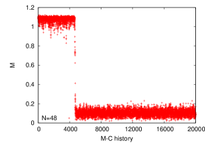
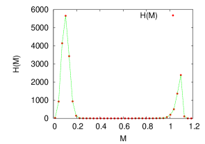
Figure 2: Monte Carlo history for N=48

Figure 3: Histogram H(M) for N=48

4.2.1 Results and discussions

In our calculations we fix $\displaystyle{R^{2}}/{N}=10$, $\displaystyle r=-8$. For simplicity we take $\displaystyle\lambda_{1}=0.25$. With this choice of parameters we do our simulations for five different sizes of the $\displaystyle\Phi$ matrices, $\displaystyle N=48,56,64,78,96$. Fig.3 gives a typical Monte-Carlo history of our simulations for $\displaystyle N=48$.

In Fig.3 $\displaystyle M$ fluctuates around a value close to the initial value. Then $\displaystyle M$ suddenly jumps to a small value and settles down. A histogram $\displaystyle H(M)$ of $\displaystyle M$ clearly shows two peaks $\displaystyle M$ as seen in Fig.3. The peak on the left has large $\displaystyle l=0$ and small $\displaystyle l=1$ component. The peak at higher value of $\displaystyle M$ has large $\displaystyle l=1$ component and small $\displaystyle l=0$. This peak is close to the value of the initial configuration. So in this state fluctuations modify the initial configuration slightly and retain its topological nature. In our Monte-Carlo history we observed the $\displaystyle l=1$ state decaying to $\displaystyle l=0$ state but not vice-versa. This implies that due to finite volume effects, the uniform condensate is more stable than our initial hedgehog configuration for this case of $\displaystyle N=48$.

To study the stability of the $\displaystyle l=1$ configuration we considered both the commutative and non-commutative limit. For the commutative limit we fixed $\displaystyle R^{2}$ and considered higher values of $\displaystyle N$. We did not observe any change in the distribution of $\displaystyle M$ in the $\displaystyle l=1$ state. The average value, and the fluctuations of $\displaystyle M$ remain almost the same as we go from $\displaystyle N=48\rightarrow 64$, as can be seen in Fig.5. As for $\displaystyle N=48$ the $\displaystyle l=1$ configuration also decays for $\displaystyle N=64$. This result suggests that the $\displaystyle l=1$ topological configuration is not stable in the commutative continuum limit as expected.

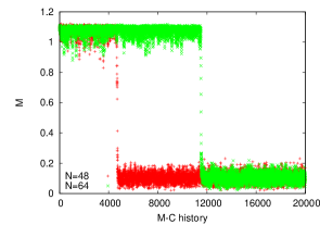
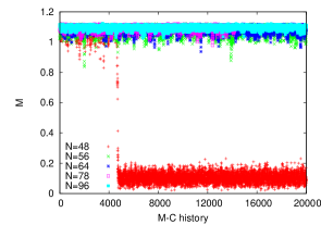
Figure 4: M-C history for fixed $\displaystyle R^{2}$

Figure 5: M-C history for fixed $\displaystyle R^{2}/N$

There is a complete change in the behavior as we consider the non-commutative limit, i.e fixed $\displaystyle{R^{2}}/{N}$ as we increase $\displaystyle N$. Except for the lowest $\displaystyle N=48$ the $\displaystyle l=1$ state did not decay during the entire run for higher $\displaystyle N$. In Fig.5 we show the Monte-Carlo history of $\displaystyle N=48,64,96$. Unlike the commutative limit, the fluctuations of $\displaystyle M$ decrease with $\displaystyle N$. In Fig.7, we give the average value of $\displaystyle M$ as a function of $\displaystyle N$. The average value of $\displaystyle M$ increases slightly with $\displaystyle N$, with the variation decreasing with $\displaystyle N$. This suggests $\displaystyle M$ will reach a finite value in the continuum limit. We also compute the fluctuations of $\displaystyle M$ to see any possible scaling with the cut-off $\displaystyle N$. In Fig.7, we show $\displaystyle\chi~{}=~{}\left<M^{2}\right>-\left<M\right>^{2}$ in the $\displaystyle l=1$ state. The solid curve represents a fit, $\displaystyle f(N)\sim N^{\alpha}$ with $\displaystyle\alpha\sim-4.$. This clearly suggest that the $\displaystyle l=1$ state is stable in the $\displaystyle N\rightarrow\infty$ leading to spontaneous breaking of the $\displaystyle O(3)$ symmetry.

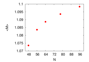
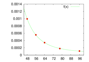
Figure 6: $\displaystyle\left<M\right>$ vs $\displaystyle N$

Figure 7: $\displaystyle\chi$ vs $\displaystyle N$

We also mention here that one can start with an initial uniform $\displaystyle l=0$ configuration and consider fluctuations. We expect that the results be similar to that in ref.[11]. In ref.[11] it was found that only the highest mode $\displaystyle l={(N-1)}/{2}$ condenses. The fact that we find the $\displaystyle l=1$ mode stable clearly shows that the topological nature of the initial configuration complements the effect of non-locality. These two effects drastically reduce the fluctuations.

4.3 Fuzzy blackholes: NC cylinder

The model defined by the action Eqs.(23,27) which we want to simulate has three parameters $\displaystyle(\mu,c,r)$ plus the matrix size $\displaystyle J$. The goal is to explore the parameter space for various phases of $\displaystyle\Phi$. The simulations are carried out using the ”pseudo-heat bath” Monte-Carlo (MC) algorithm [10, 11] to reduce the auto-correlation along the MC history.

The field should also be allowed to explore the whole phase space and not remain trapped in local minima. To this end, an over-relaxation method, first suggested in [9], is also used. Let us introduce $\displaystyle S_{\Phi}(\Phi_{ij})$ the dependence of the action on the field entry $\displaystyle\Phi_{ij}$ when the field takes the value $\displaystyle\Phi$. It is a fourth degree polynomial. Therefore the equation $\displaystyle S_{\Phi}(\Phi_{ij})=S_{\Phi}(\Phi_{ij}=a)$, which has an obvious solution $\displaystyle\Phi_{ij}=a$, can be factorised into a degree three polynomial which always admits at least one real solution. The overrelaxation method consists in replacing the field entry $\displaystyle\Phi_{ij}=a$ by one of these real solutions, thereby moving the field in a different region of the phase space. A crosscheck is also used to verify that the field probability distribution of our Monte-Carlo runs are consistent. Let us split the terms in the action according to their scalings

$$S(\phi)=S_{2}(\phi)+S_{4}(\phi)\mbox{ with }S_{i}(\lambda\phi)=\lambda^{i}S_{i}(\phi).$$

Then one can define a modified partition function

$$\displaystyle Z(\lambda)=\int[\mathrm{d}\phi]e^{-S(\lambda\phi)} \displaystyle= \displaystyle\int[\mathrm{d}\phi]e^{-\lambda^{2}S_{2}(\phi)-\lambda^{4}S_{4}(\phi)}$$ (35)

$$\displaystyle= \displaystyle\lambda^{-N}\int[\mathrm{d}\psi]e^{-S(\psi)},\ \psi=\lambda\phi,$$ (36)

where $\displaystyle N$ is the number of degrees of freedom in the field $\displaystyle\phi$ which appear in the integration. Evaluating

$$\displaystyle\left.\frac{\partial\ln(Z)}{\partial\lambda}\right|_{\lambda=1} \displaystyle= \displaystyle-2<S_{2}>-4<S_{4}>\mbox{ from (\ref{Z1})}$$

$$\displaystyle= \displaystyle-N\mbox{ from (\ref{Z2})}$$

yields the check originally due to Denjoe O’Connor [39].

$$<S_{2}>+2<S_{4}>=N/2$$ (37)

In all simulations, this identity (37) is always satisfied to better than $\displaystyle 1\%$ relative error.

4.3.1 The phase structure

The temperature ($\displaystyle T$) is regulated by varying the parameter $\displaystyle\mu$.

• $\displaystyle\mu\ll 1$ corresponds to low temperatures when the fluctuations are small. In this case, the minimum of $\displaystyle S$ gives the most probable configuration of the phase. In Eq. (27), it is possible to minimise the action by minimising separately the kinetic term, so that $\displaystyle\Phi\propto{\bf 1}$, and the potential term so that $\displaystyle\Phi=\sqrt{-\mu/2c}\,{\bf 1}$, and this phase is therefore known as the uniform phase.

• At high temperatures, $\displaystyle\mu\gg 1$, the thermal fluctuations lead the system to the disorder phase $\displaystyle\Phi\sim 0$.

• At intermediate temperatures, the competition between the action and the fluctuations give rise to new phases called the non-uniform or stripe phases. These new phases are specific to non-commutative spaces. Various numerical studies have confirmed the existence of these phases [6, 7, 9, 10, 11, 8, 14, 13] on the fuzzy sphere. A non-commutative cylinder will also exhibit the non-uniform phases. However, due to the non-trivial topology of the cylinder (the first homotopy group being non-trivial), one can have a more complex phase structure described below.

For example there can be stripes going around the cylinder, or parallel to its axis. These two phases can be distinguished by their overlap with the operators $\displaystyle Z$, $\displaystyle{e^{i\phi}}$, and $\displaystyle{e^{i\phi}}^{\dagger}$ respectively. Stripes going around the cylinder will have non-zero overlap with the operator $\displaystyle Z$. While a configuration of stripes along the axis will have overlap with $\displaystyle{e^{i\phi}}$ and $\displaystyle{e^{i\phi}}^{\dagger}$. We present our results in the following subsection.

4.3.2 Example numerical runs

For a given choice of $\displaystyle N=7$, $\displaystyle c=0.36$, and $\displaystyle r=1$ the simulations are done for various values of $\displaystyle\mu$. The various phases discussed above can be characterised by the observables $\displaystyle m_{u}=Tr(\Phi)$, $\displaystyle m_{z}=Tr(\Phi Z)$, $\displaystyle m_{x}=Tr(\Phi e^{i\phi})$. A finite $\displaystyle m_{u}$ with $\displaystyle(m_{z},m_{x})\sim 0$ characterizes the uniform phase. On the other hand, $\displaystyle(m_{u},m_{x})\sim 0$ with non-zero $\displaystyle m_{z}$ characterizes stripes going around the cylinder. Stripes along the cylinder charactersied by $\displaystyle(m_{u},m_{z})\sim 0$ with non-zero $\displaystyle m_{x}$.

For $\displaystyle\mu=-35.1$, the data of a run are shown on Fig.9, and, as expected, we observe the uniform phase.

For $\displaystyle\mu=-20.0$, we observed the phase with stripes going around the cylinder. This is verified on the histogram of the observed values of $\displaystyle m_{u},m_{z}$ plotted in Fig.9. It is clear from the figure that the average value of $\displaystyle m_{z}$ is finite while the average value of $\displaystyle m_{u}$ is vanishingly small.

Fig.11 shows the system in the disorder phase where $\displaystyle m_{u},m_{z},m_{x}$ all fluctuate around zero. We did not observe the phase with stripes going along the cylinder as a ground state for any choice of $\displaystyle\mu$ for $\displaystyle r\sim 1$. One can expect to observe this state for very small $\displaystyle r$ when the second term which suppresses this state is made subdominant. For a very small radius $\displaystyle r=0.01$, $\displaystyle c=36.$ and $\displaystyle\mu=-3.6\times 10^{3}$, this phase appears as meta-stable in Fig.11. This phase is stable w.r.t small fluctuations. Only large fluctuations, which occur less frequently, can destroy such a state.

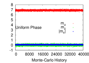
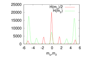
Figure 8: $\displaystyle m_{u,z,x}$ vs MC history $\displaystyle N=7,\mu=-35.1,c=.36$

Figure 9: Histogram of $\displaystyle H(m_{u}),H(m_{z}):N=7,\mu=-20$

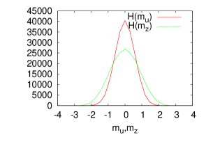
Figure 10: Histogram of $\displaystyle H(m_{u}),H(m_{z}):N=7=0.36$

Figure 11: $\displaystyle m_{u,z,x}$ vs MC history $\displaystyle N=7,\mu=-3.6\times 10^{3},c=36,r=.01$

5 Conclusions

In this analysis we have shown that topologically non-trivial configurations on the fuzzy sphere avoid the CMW theorem much more dramtically than the non-topological symmetry breaking [40]. The mass gap or the infrared cut-off in this case is large enough to render the fluctuations of the Goldstone modes finite. On the other hand for non-topological condensates the Goldstone modes are large enough to destroy almost all the modes except the few highest modes. We have presented the simulations wherein the cubic Chern-Simons (CS) term is absent in the action Eq (18). The Chern-Simons term allows topological solitons even when the quadratic mass term is positive upto some value. Interestingly with CS term the configuration $\displaystyle\phi_{i}~{}=~{}\alpha~{}L_{i}$ is preferred over symmetric solution. On the otherhand, it is not expected to alter the picture of topological stability of the solutions. This term plays an important role in the emergent geometry in NC fuzzy spaces [41, 42]. What we find here in the simulations is that even in the absence of CS term, emergent fuzzy spaces can be stable. The stabilty of higher dimensional fuzzy spaces like $\displaystyle CP_{F}^{2}$ are of significance in this context [43]. The implications of this stability for extra-dimensional fuzzy spaces will be considered later.

We have also considered a finite dimensional representations of the noncommutative cylinder algebra, which make it fuzzy. We study scalar field theory in the background of this algebra both analytically and using numerical simulations.

In the numerical simulations of scalar field with a generic potential we find, as expected in noncommutative cylinder, novel stripe phases breaking translational symmetry. But they have some differences with the usual stripes on Moyal spacetimes. These are also stable due to topological features arising in this fuzzy geometry.

It is well known that a large class of noncommutative black holes are described by a noncommutative cylinder algebra. The fuzzy cylinder algebra derived from it can therefore be used to define a fuzzy black hole. From general considerations[1] we know that such black holes can arise at the Planck scale. Our results provide a first glimpse about the phase structure of a quantum scalar field theory in the background of a fuzzy black hole at the Planck scale [44].

Acknowledgment This work was done as a part of the CEFIPRA/IFCPAR project 4004-1 entitled Fuzzy Approach to Quantum Field Theory and Gravity. The authors gratefully acknowledge the financial assistance from CEFIPRA/IFCPAR which was essential for this work.

References

- [1] S. Doplicher, K. Fredenhagen and J. E. Roberts, Commun. Math. Phys. 172 (1995) 187.
- [2] P. Podles, E. Muller, Rev. Math. Phys. 10 (1998), 511-551 [arXiv:q-alg/9704002v2]
- [3] “On the hypotheses which lie at the bases of geometry”, Bernhard Riemann, 1854 (from the translation by W K Clifford)
-
[4]
A.P. Balachandran, T.R. Govindarajan and B. Ydri,
Mod. Phys. Lett. A15 (2000) 1279 [hep-th/9911087];
A.P. Balachandran, A. Pinzul and B.A. Qureshi, JHEP 0512 (2005) 002 [hep-th/0506037]. - [5] S.S. Gubser and S.L. Sondhi, Nucl. Phys. B605, 395 (2001) [hep-th/0006119].
- [6] X. Martin, JHEP 0404 (2004) 077 [hep-th/0402230].
-
[7]
J. Medina, W. Bietenholz, F. Hofheinz and
D. O’Connor, PoS LAT2005 (2005) 263 [hep-lat/0509162];
F. G. Flores, D. O’Connor and X. Martin, PoS LAT2005 (2006) 262 [hep-lat/0601012];
D. O’Connor and B. Ydri, JHEP 0611 (2006) 016 [hep-lat/0606013];
J. Medina, Phd. thesis, arXiv: 0801.1284 [hep-th]. -
[8]
W. Bietenholz, F. Hofheinz and J. Nishimura,
Acta. Phys. Polon. B34 (2003) 4711 [hep-th/0309216];
Nucl. Phys. Proc. Suppl. 129 (2004) 865 [hep-th/0309182]. -
[9]
M. Panero, SIGMA 2 (2006) 081 [hep-th/0609205];
JHEP 0705, 082 (2007) [hep-th/0608202]. - [10] C.R. Das, S. Digal and T.R. Govindarajan, Mod. Phys. Lett. A23 (2008) 1781.
- [11] C.R. Das, S. Digal and T.R. Govindarajan, Mod. Phys. Letts A24 (2009) 2693.
- [12] T R Govindarajan and E Harikumar, Phys. Letts., B 602 (2004) 238; A P Balachandran and G Immirzi, Int Jour. Mod. Phys. A19 (2004) 5237.
- [13] J. Ambjorn and S. Catterall, Phys. Lett. B549 (2002) 253 [hep-lat/0209106].
- [14] J. Medina, W. Bietenholz and D. O’Connor, JHEP 0804, (2008) 041; arXiv:0712.3366 [hep-th].
- [15] P. Aschieri, C. Blohmann, M. Dimitrijevic, F. Meyer, P. Schupp and J. Wess, Class. Quant. Grav. 22 (2005) 3511.
- [16] A.P. Balachandran, T.R. Govindarajan, K.S. Gupta, S. Kurkcuoglu, Class. Quant. Grav. 23 (2006) 5799.
- [17] B.P. Dolan, Kumar S. Gupta and A. Stern, Class. Quant. Grav. 24 (2007) 1647.
- [18] P. Schupp and S. Solodukhin, arXiv:0906.2724 [hep-th].
- [19] T. Ohl and A. Schenkel, JHEP 0910 (2009) 052.
- [20] M. Banados, C. Teitelboim and J. Zanelli, Phys. Rev. Lett. 69 (1992) 1849.
- [21] M. Banados, M. Henneaux, C. Teitelboim and J. Zanelli, Phys. Rev. D 48 (1993) 1506.
- [22] H. Grosse and P. Presnajder, Acta Phys. Slovaca 49 (1999) 185.
- [23] J. Lukierski, A. Nowicki, H. Ruegg and V. N. Tolstoy, Phys. Lett. B 264 (1991) 331.
- [24] J. Lukierski, H. Ruegg and W. J. Zakrzewski, Ann. Phys. 243 (1995) 90.
- [25] S. Meljanac and M. Stojić, Eur. Phys. J. C 47 (2006) 531.
- [26] S. Meljanac, A. Samsarov, M. Stojić and K. Gupta, Eur. Phys. J. C 53 (2008) 295.
- [27] M. Daszkiewicz, J. Lukierski and M. Woronowicz, J. Phys. A 42 (2009) 355201.
- [28] J. Lukierski, Rept. Math. Phys. 64 (2009) 299.
- [29] T. R. Govindarajan, K. S. Gupta, E. Harikumar, S. Meljanac and D. Meljanac, Phys. Rev. D 77 (2008) 105010.
- [30] T. R. Govindarajan, K. S. Gupta, E. Harikumar, S. Meljanac and D. Meljanac, Phys. Rev. D 80 (2009) 025014.
- [31] T.R.Govindarajan, Kumar S. Gupta, E. Harikumar and S. Meljanac, Journal of Physics: Conference Series 306 (2011) 012019.
- [32] Kumar S. Gupta, S. Meljanac and A. Samsarov, arXiv:1108.0341 [hep-th]
- [33] M. Chaichian, A. Demichev, P. Presnajder and A. Tureanu, Phys. Lett. B 515 (2001) 426.
- [34] A. P. Balachandran, T. R. Govindarajan, A. G. Martins and P. Teotonio-Sobrinho, JHEP 0411 (2004) 068; A. P. Balachandran, T. R. Govindarajan, C. Molina, P. Teotonio-Sobrinho, JHEP 0410 (2004) 072.
- [35] J. Madore, An Introduction to Noncommutative Differential Geometry and its Physical Applications, (London Mathematical Society Lecture Note Series).
- [36] A.P. Balachandran, S. Kurkcuoglu and S. Vaidya, Lectures on fuzzy and fuzzy SUSY physics, World Scientific (2007).
- [37] T.R.Govindarajan, Pramod Padmanabhan and T.Shreecharan J. Phys.A43 (2010) 205203.
- [38] J. Arnlind, M. Bordemann, L. Hofer, J. Hoppe and H. Shimada JHEP 0906 (2009) 047.
- [39] Denjoe O’Connor (private communication)
- [40] S. Digal and T. R. Govindarajan, arXiv:1108.3320 [hep-th]
- [41] Harold Steinacker, Nucl. Phys. B810 (2009) 1
- [42] Rodrigo-Delgadillo Blando, Denjoe O’Connor, B Ydri, Phys. Rev. Letts, 100 (2008) 201601.
- [43] Brian P Dolan, Idrish Huet, Sean Murray, Denjoe O’Connor, JHEP0707 (2007) 007.
- [44] S. Digal, T. R. Govindarajan, Kumar S. Gupta and X. Martin JHEP 1201 (2012) 027 arXiv:1109.4014 [gr-qc].