APPROACHING THE PROBLEM OF TIME

WITH A COMBINED SEMICLASSICAL-RECORDS-HISTORIES SCHEME

Edward Anderson^∗

APC AstroParticule et Cosmologie, Université Paris Diderot CNRS/IN2P3, CEA/Irfu, Observatoire de Paris, Sorbonne Paris Cité, 10 rue Alice Domon et Léonie Duquet, 75205 Paris Cedex 13, France.

and DAMTP, Centre for Mathematical Sciences, Wilberforce Road, Cambridge CB3 OWA

I approach the Problem of Time and other foundations of Quantum Cosmology using a combined histories, timeless and semiclassical approach. This approach is along the lines pursued by Halliwell. It involves the timeless probabilities for dynamical trajectories entering regions of configuration space, which are computed within the semiclassical regime. Moreover, the objects that Halliwell uses in this approach commute with the Hamiltonian constraint, H. This approach has not hitherto been considered for models that also possess nontrivial linear constraints, Lin. This paper carries this out for some concrete relational particle models (RPM’s). If there is also commutation with Lin – the Kuchař observables condition – the constructed objects are Dirac observables. Moreover, this paper shows that the problem of Kuchař observables is explicitly resolved for 1- and 2-$d$ RPM’s. Then as a first route to Halliwell’s approach for nontrivial linear constraints that is also a construction of Dirac observables, I consider theories for which Kuchař observables are formally known, giving the relational triangle as an example. As a second route, I apply an indirect method that generalizes both group-averaging and Barbour’s best matching. For conceptual clarity, my study involves the simpler case of Halliwell 2003 sharp-edged window function. I leave the elsewise-improved softened case of Halliwell 2009 for a subsequent Paper II. Finally, I provide comments on Halliwell’s approach and how well it fares as regards the various facets of the Problem of Time and as an implementation of QM propositions.

^∗ eanderso@apc.univ-paris7.fr

1 Introduction

1.1 The Problem of Time and its Frozen Formalism Facet

This notorious problem [2, 3, 4, 5, 6, 7, 8, 9, 10, 11, 12, 13, 14, 15] occurs because the ‘time’ of GR and the ‘time’ of ordinary Quantum Theory are mutually incompatible notions. This incompatibility leads to a number of problems with trying to replace these two branches with a single framework in situations in which the premises of both apply, such as in black holes and in the very early universe. This is investigated in this paper via relational particle models (RPM’s) [16, 17, 18, 19, 20, 21, 22, 23, 24, 25, 26, 27, 28, 29, 30, 31, 32, 33, 34, 35, 36, 37, 14, 38, 39, 40]. Sec 1.5 explains the nature of these models. For now, I note that they have a large number of analogies with GR (see [6, 17, 18, 11, 21, 12, 29, 30, 31, 32, 33, 34] and especially [14]), rendering them suitable as toy models for many aspects of the Problem of Time.

One notable facet of the Problem of Time shows up in attempting canonical quantization of GR (or of many other gravitational theories that carry over likewise background-independent). It is due to GR’s Hamiltonian constraint

$${\cal H}:={\cal N}_{\mu\nu\rho\sigma}\pi^{\mu\nu}\pi^{\rho\sigma}/\sqrt{h}-\sqrt{h}\{\mbox{Ric}(x;h]-2\Lambda\}=0\mbox{ }$$ (1)

being quadratic but not linear in the momenta; I denote the general case of such a constraint by ${\cal Q}$uad.

Then promoting a constraint with a momentum dependence of this kind to the quantum level gives a time-independent wave equation

$$\widehat{\cal H}\Psi=0\mbox{ },$$ (2)

in place of ordinary QM’s time-dependent one,

$$i\partial\Psi/\partial t=\widehat{\mbox{H}}\Psi\mbox{ }$$ (3)

[or a functional derivative $\delta/\delta t(x^{\mu})$ counterpart of this in the general GR case]. Here, H is a Hamiltonian, $\Psi$ is the wavefunction of the universe and $t$ is absolute Newtonian time [or a a local GR-type generalization $t(x^{\mu})$].

In the case of GR, in more detail, (2) is a Wheeler–DeWitt equation,

$$\widehat{\cal H}\Psi:=-\mbox{`}\left\{\frac{1}{\sqrt{{\cal M}}}\frac{\delta}{\delta h^{{\mu\nu}}}\left\{\sqrt{{\cal M}}{\cal N}^{\mu\nu\rho\sigma}\frac{\delta\Psi}{\delta h^{{\rho\sigma}}}\right\}-\xi\,\mbox{Ric}(h;{\cal M}]\right\}\mbox{'}\,\Psi-\sqrt{h}\mbox{Ric}(x;h]\Psi+{\sqrt{h}2\Lambda}\Psi=0\mbox{ }.$$ (4)

This suggests, in apparent contradiction with everyday experience, that nothing at all happens in the universe! Thus one is faced with having to explain the origin of the notions of time in the laws of physics that appear to apply in the universe. Sec 1.3 considers a number of strategies toward explaining this. [Moreover timeless equations such as the Wheeler–DeWitt equation apply to the universe as a whole, whereas the more ordinary laws of physics apply to small subsystems within the universe, suggesting this to be an apparent ‘paradox’ rather than an actual one.]

1.2 Other Facets of the Problem of Time

Over the past decade, it has become more common to suggest or imply that the Problem of Time is the Frozen Formalism Problem. However, a more long-standing point of view [5, 6, 7, 8] (and also argued in favour for in e.g. [9, 11, 13, 14, 15] and the present article) is that the Problem of Time contains a number of further facets. Furthermore, this is not even a case of then having to address around eight facets in succession. For, as Kuchař found, these facets interfere with each other. He termed this [8] a ‘many gates’ problem, in which one attempting to enter the gates in sequence finds that they are no longer inside some of the gates they had previously entered. I argue that this occurs because the facets arise from a common cause – the mismatch of the notions of time in GR and Quantum Theory – by which they bear conceptual and technical relations, making it advantageous, and likely necessary for genuine progress, to treat them as a coherent package rather than piecemeal as ‘unrelated problems’. To emphasize this common cause, and place the eight principal facets into a more memorable form (I have found most theoreticians to be unaware of some facets and/or of their time connotations), I used an even more vivid mnemonic [13, 14], depicting the eight facets as the breath, wings, tail, scales and four sets of claws that constitute a single entity: the Ice Dragon. This depiction makes it clear that the eight facets inter-protect each other (as Kuchař observed), so that resolving the Problem of Time is altogether harder than addressing each of the facets in succession, let alone just unfreezing the equations of physics.

Apart from the ‘frozen breath’, only the ‘wings’ of the Problem of Observables shall play a recurring theme in the present article. The Frozen Formalism Facet itself has the following addendum.

Hilbert Space/Inner Product Problem, i.e. how to turn the space of solutions of the frozen equation in question into a Hilbert space. In GR, indefiniteness of the kinetic metric prevents use of a Schrödinger inner product and then a Klein–Gordon type one fails on other grounds [4]. This is a time problem since inner products and unitary evolution are tied.

We next require an interlude so as to interpret further facets. GR also has a linear momentum constraint

$${\cal H}_{\mu}:=-2D_{\nu}\pi^{\nu}\mbox{}_{\mu}=0\mbox{ }\mbox{ which becomes, at the quantum level, }\mbox{ }\widehat{\cal H}_{\mu}\Psi:=-2D_{\rho}h^{\rho\nu}\delta\Psi/\delta h_{\mu\nu}=0\mbox{ };$$ (5)

this often becomes entwined in technical problems that afflict Problem of Time strategies.

Many such entwinings (see e.g. the next two Problems below) furthermore specifically concern diffeomorphisms [whether i) the spatial diffeomorphisms associated with the GR momentum constraint itself, ii) the spacetime diffeomorphisms or iii) the result splitting the spacetime diffeomorphisms due to a foliation by spatial hypersurfaces as occurs in canonical approaches to GR]. iii) is altogether harder to handle; whilst i) and ii) are both infinite-dimensional Lie groups, in iii) the GR Hamiltonian constraint does not directly account for the diffeomorphisms of ii) that are not present amongst those of i) This is reflected e.g. in the Dirac algebra of the GR constraints having not the mere structure constants of a Lie algebra but, rather, structure functions. At least this algebra does retain the useful property of closing at the classical level without further constraints appearing. Additionally, in classical GR, one can foliate spacetime in many ways, each corresponding to a different choice of timefunction. This is how time in classical GR comes to be ‘many-fingered’, with each finger ‘pointing orthogonally’ to each foliation. Finally, classical GR has the remarkable property of being foliation-independent [48], so that going between two given spatial geometries by means of different foliations in between produces the same region of spacetime, thus giving the same answers to whatever physical questions can be posed therein. Equipped with this knowledge, one can return to the discussion of the Problem of Time.

Best Matching Problem: I argued in [14, 38, 15] that this is a more general conceptualization of, and name for, the usually-listed Sandwich Problem. The context for this is that, if the theory has $\mathfrak{g}$-nontriviality for $\mathfrak{g}$ the group associated with the linear constraints ${\cal L}\mbox{i}\mbox{n}_{\mbox{{\scriptsize Z}}}$ [generalization of (5)], then varying with respect to the auxiliary $\mathfrak{g}$-variables produces ${\cal L}$in${}_{\mbox{{\scriptsize Z}}}$. The Best Matching Problem is then whether one can solve the Lagrangian form of ${\cal L}\mbox{i}\mbox{n}_{\mbox{{\scriptsize Z}}}=0$ for the $\mathfrak{g}$-auxiliaries themselves, which is a particular form of reduction. This problem is clearly already present at the classical level. It furthermore becomes entwined in some of the approaches that start with manipulations at the classical level prior to quantizing.

Foliation Dependence Problem: for all that one would like a quantization of GR to retain the nice classical property of refoliation invariance, at the quantum level there ceases to be an established way of guaranteeing this property. That this is obviously a time problem follows from each foliation by spacelike hypersurfaces being orthogonal to a GR timefunction: each slice corresponds to an instant of time for a cloud of observers distributed over the slice. Each foliation corresponds to such a cloud of observers moving in a particular way.

Functional Evolution Problem alias Possibility of Anomalies. This is the quantum-level problem that the commutator of constraints is capable of manifesting, involving breakdown of the immediate closure of the constraint algebra that occurs at the classical level. Dirac [46] said that one had to be lucky so as to avoid such breakdowns. Note that only some of the anomalies that one finds in physics are time-related. However, in the present case of the quantum counterpart of the Dirac algebra of GR constraints, this is a time issue due to what these constraints signify. In particular, non-closure here is a way in which the Foliation Dependence Problem can manifest itself, through the non-closure becoming entwined with details of the foliation. [Non-closure is also entwined with the Operator Ordering Problem, since changing the operator ordering gives additional right-hand-side pieces not present in the classical Poisson brackets algebra.]

Multiple Choice Problem alias Kuchař’s Embarrassment of Riches [6]. This is the purely quantum-mechanical problem that different choices of time variable may give inequivalent quantum theories. [The ‘riches’ are then the multiplicity of such inequivalent quantum theories.] Foliation Dependence is one of the ways in which the Multiple Choice Problem can manifest itself. Moreover, the Multiple Choice Problem is known to occur even in some finite toy models, so that foliation issues are not the only source of the Multiple Choice Problem. For instance, another way the Multiple Choice Problem can arise is as a subcase of how making different choices of sets of variables to quantize may give inequivalent quantum theories, as follows from e.g. the Groenewold–van Hove phenomenon.

Global Problem of Time alias Kuchař’s Embarrassment of Poverty [6]. This is already present at the classical level. The spatial part of this problem consists in the separation into true variables and embedding (space frame and timefunction) variables’ having a proneness for being globally impossible, for reasons that closely parallel the Gribov effect in Yang–Mills theory. This proneness to not globally exist explains Kuchař’s name for this problem. The temporal part of this problem concerns cases in which such a split can be defined but cannot be indefinitely continued as one progresses along a foliation (or simpler models’ timefunctions eventually going astray).

Spacetime (Reconstruction or Replacement) Problem [6, 15]. Internal space or time coordinates to be used in the conventional classical spacetime context need to be scalar field functions on the spacetime 4-manifold. In particular, these do not have any foliation dependence. However, the canonical approach to GR uses functionals of the canonical variables, and which there is no a priori reason for such to be scalar fields of this type. Thus one is faced with either finding functionals with this property, or coming up with a new means of reducing to the standard spacetime meaning at the classical level. There are further issues involving properties of spacetime being problematical at the quantum level. Quantum Theory implies fluctuations are unavoidable, but now that these amount to fluctuations of 3-geometry, they are too numerous to fit within a single spacetime (see e.g. [3]). Thus (something like) the superspace picture (considering the set of possible 3-geometries) might take over from the spacetime picture at the quantum level. It is then not clear what becomes of causality (or of locality, if one believes that the quantum replacement for spacetime is ‘foamy’ [3]). There is also an issue of recovering continuity in suitable limits in approaches that treat space or spacetime as discrete at the most fundamental level (see e.g. [49]).

Problem of Beables. This is usually called the Problem of Observables [46, 6, 7, 10], but I follow Bell [50, 51] in ascribing more physical significance to beables than to observables, especially in the context of Quantum Cosmology. I prefer to use beables, or yet other names corresponding to local versions of such concepts, as per Sec 8.2. The Problem of Beables involves construction of a sufficient set of beables for the physics of one’s model; there are then involved in the model’s notion of evolution. The Problem of Beables was depicted [14] as the ‘wings’ of the Ice Dragon, due to observables/beables issues popping up all over the place in Theoretical Physics, much like that the Ice Dragon suddenly popping up in unexpected places of the realm through having wings to swiftly and unexpectedly fly there). Though, as we shall see in Sec 2, ‘whether the Ice Dragon has wings’ remains a debated point.

1.3 A selection of Problem of Time strategies

A) Semiclassical Approach. Perhaps one has slow, heavy ‘h’ variables that provide an approximate timestandard with respect to which the other fast, light ‘l’ degrees of freedom evolve [52, 6, 11]. In the Halliwell–Hawking [52] scheme for GR Quantum Cosmology, $h$ is scale (and homogeneous matter modes) and the l-part are small inhomogeneities. I.e., it is a perturbative midisuperspace model. The Semiclassical Approach involves making

$$\mbox{i) the Born--Oppenheimer (BO) ansatz}\hskip 72.26999pt\Psi(\mbox{h},\mbox{l})=\psi(\mbox{h})|\chi(\mbox{h},\mbox{l})\rangle\mbox{ },\hskip 289.07999pt$$ (6)

$$\mbox{ii) the WKB ansatz}\hskip 155.38005pt\psi(\mbox{h})=\mbox{exp}(i\,S(\mbox{h}))\mbox{ };\hskip 361.34999pt$$ (7)

in each case one makes a number of associated approximations. [Evoking semiclassicality only makes sense if one’s goals are somewhat modest as compared to some more general goals in Quantum Gravity programs. Nevertheless this is still useful for some applications, including the foundations of practical Quantum Cosmology i.e. putting calculations along the lines of Halliwell and Hawking’s.]

iii) One forms the h-equation, $\langle\chi|\widehat{\cal H}\Psi=0.$ Then, under a number of simplifications, this yields a Hamilton–Jacobi equation $\{\partial S/\partial\mbox{h}\}^{2}=2\{E-V(\mbox{h})\}$ , where $V(\mbox{h})$ is the h-part of the potential and $E$ is the total energy.

One way of solving this involves doing so for an approximate emergent semiclassical time $t^{\mbox{\scriptsize e}\mbox{\scriptsize m}(\mbox{\scriptsize W}\mbox{\scriptsize K}\mbox{\scriptsize B})}(\mbox{h})$; this happens to be [22, 14] a recovery of a ‘time before quantization’ timefunction: the Jacobi–Barbour–Bertotti one [16, 17].

iv) One then forms the l-equation $\{1-|\chi\rangle\langle\chi|\}\widehat{\cal H}\Psi=0$. This is a fluctuation equation but it can be recast (modulo further approximations) into a $t^{\mbox{\scriptsize e}\mbox{\scriptsize m}(\mbox{\scriptsize J}\mbox{\scriptsize B}\mbox{\scriptsize B})}$-dependent Schrödinger equation for the l-degrees of freedom,

$$i\partial|\chi\rangle/\partial t^{\mbox{\scriptsize e}\mbox{\scriptsize m}}=\widehat{\mbox{H}}_{\mbox{\scriptsize l}}|\chi\rangle\mbox{ }\mbox{ }.$$ (8)

The emergent time dependent left-hand side of this arises from the cross-term $\partial_{\mbox{\scriptsize h}}|\chi\rangle\partial_{\mbox{\scriptsize h}}\psi$. $\widehat{\mbox{H}}_{\mbox{\scriptsize l}}$ is the remaining surviving piece of $\widehat{\cal H}$, acting as a Hamiltonian for the l-subsystem. Moreover, the working leading to such a time-dependent wave equation ceases to function in the absence of making the WKB ansatz and approximation, which, additionally, in the quantum-cosmological context, is not known to be a particularly strongly supported ansatz and approximation to make.

B) Timelessness. A number of approaches take timelessness at face value. One considers only questions of the universe ‘being’, rather than ‘becoming’, a certain state.

B.1) A first example is the Naïve Schrödinger Interpretation. (This is due to Hawking and Page [45], though its name was coined by Unruh and Wald [53].) This concerns the ‘being’ probabilities for universe properties such as: what is the probability that the universe is large? Flat? Isotropic? Homogeneous? One proceeds via considering the probability that the universe belongs to region R of the configuration space that corresponds to a quantification of a particular such property,

$$\mbox{Prob}(\mbox{R})\propto\int_{\mbox{\scriptsize R}}|\Psi|^{2}\mathbb{D}\mbox{\bf Q}\mbox{ },$$ (9)

for $\mathbb{D}\mbox{\bf Q}$ the configuration space volume element. This approach is termed ‘naïve’ due to it not using any further features of the constraint equations. Its implementation of propositions is Boolean via how the region enters the integral.

B.2) The Conditional Probabilities Interpretation [54] goes further by addressing conditioned questions of ‘being’. The conditional probability of finding $B$ in the range $b$, given that $A$ lies in $a$, and to allot to it the value

$${\rm Prob}(B\in b|A\in a;\mbox{\Large$\rho$})=\frac{\mbox{tr}\big{(}\mbox{P}^{B}_{b}\,\mbox{P}^{A}_{a}\,\mbox{\Large$\rho$}\,\mbox{P}^{A}_{a}\big{)}}{\mbox{tr}\big{(}\mbox{P}^{A}_{a}\,\mbox{\Large$\rho$}\big{)}}\mbox{ },$$ (10)

where $\rho$ is a density matrix for the state of the system and the $\mbox{P}^{A}_{a}$ denote projectors. An example of such a question is ‘what is the probability that the universe is flat given that it is isotropic’? This approach can additionally deal with the question of ‘being at a time’ by having the conditioning proposition refer to a ‘clock’ subsystem.

B.3) Records Theory involves localized subconfigurations of a single instant of time. It concerns issues such as whether these contain useable information, are correlated to each other, and whether a semblance of dynamics or history arises from this (which can involve reducing questions of ‘becoming’ to questions of ‘being’). Records Theory is a heterogeneous subject, a number of different authors advocating different notions of Records Theory are Page [55], Barbour [18] and I [27, 14, 39] (see also the next SSec).

C) Histories Theory. Perhaps instead it is the histories that are primary, a view brought to the GR context by Gell–Mann and, especially, Hartle [56, 57] and subsequently worked on by Isham, Linden, Savvidou and others [59, 58, 60].

1.4 Halliwell’s combined approach

Some motivation for this is as follows.

Pro 1) Both histories and timeless approaches lie on the common ground of atemporal logic structures [58, 14].

Pro 2) There is a Records Theory within Histories Theory, as pointed out by Gell-Mann and Hartle [56] and further worked on by them [61], and by Halliwell and collaborators [62, 63, 64, 65, 66, 67, 68]. Thus Histories Theory supports Records Theory by providing guidance as to the form a working Records Theory would take. This also allows for these two to be jointly cast as a mathematically-coherent package (as already illustrated in preceding subsections). As Gell-Mann and Hartle say [56],

$$\mbox{Records are ``{\it somewhere in the universe where information is stored when histories decohere}"}.$$ (11)

Anti 1) There is some chance that being more minimalistic than Gell-Mann–Hartle and Halliwell could itself succeed. If one alternatively considers records from first principles from which histories are to be derived, as the history collapses to a single instant, path integrals cease to be defined so this kind of decoherence functional is absent from Records Theory.

Pro 3) Histories decohereing is a leading (but as yet not fully established) way by which a semiclassical regime’s WKB approximation could be legitimately obtained in the first place. Thus Histories Theory could support the Semiclassical Approach by freeing it of a major weakness.

Pro 4) The Semiclassical Approach and/or Histories Theory could plausibly support Records Theory by providing a mechanism for the semblance of dynamics [64, 11] (though the possibility of a practically useable such occurring within pure Records Theory has not been overruled). Such would go a long way towards Records Theory being complete. N.B. that emergent semiclassical time amounts to an approximate semiclassical recovery [22] of Barbour’s classical emergent time [17, 39, 40], which is an encouraging result as regards making such a Semiclassical–Timeless Records combination.

Pro 5) The elusive question of which degrees of freedom decohere which should be answerable through where in the universe the information is actually stored, i.e. where the records thus formed are [56, 64]. In this way, Records Theory could in turn support Histories Theory.

Pro 6) The Semiclassical approach aids in the computation of timeless probabilities of histories entering given configuration space regions. This is by the WKB assumption giving a semiclassical flux into each region [64] in terms of $S(\mbox{h})$ and the Wigner function (defined in Sec 3). Such schemes go beyond the standard Semiclassical Approach, and as such there may be some chance that further objections to the Semiclassical Approach (problems inherited from the Wheeler–DeWitt equation and Spacetime Reconstruction Problems) would be absent from the new unified strategy.

Pro 7) Halliwell’s approach has further foundational value for practical Quantum Cosmology.

For details of the parts of Halliwell’s program considered in this paper, see Sec 3.

Note 1) This program does not make further use of the Semiclassical Approach’s specific unfreezing moves, for all that it does use BO-WKB approximations in obtaining various expressions relevant to the Problem of Time.

Note 2) Halliwell’s approach’s attitude to observables/beables is a Dirac one (see Sec 2), though he does not for now consider the effect of linear constraints; the present paper’s study is the first to consider examples possessing linear constraints.

1.5 Outline of relational particle mechanics (RPM’s)

RPM’s are whole-universe models, toy models of geometrodynamics, with nontrivial constraints and structure formation. These are suitable for the study of Quantum Cosmology and some Problem of Time aspects. In particular, they are a good arena for Histories, Records and Semiclassical Approaches, and quite possibly observables/beables based approaches too (a point toward which the present paper contributes). RPM’s obey the following ‘Leibniz–Mach–Barbour’ brand of relationalism (GR can be cast in a closely parallel form too [69, 14]).

A physical theory is temporally relational if there is no meaningful primary notion of time for the system as a whole (e.g. the universe) [16, 69, 24, 38]. The very cleanest implementation of this is by using actions that are i) manifestly parametrization irrelevant, and ii) free of extraneous time-related variables. [E.g. one is not to involve external absolute Newtonian time, or the dynamical formulation of GR’s ‘lapse’ variable.] The relational action that implements the above in the case of RPM’s is the Jacobi-type action

$$S=\sqrt{2}\int\textrm{d}s\sqrt{E-V}\mbox{ },$$ (12)

for $\textrm{d}s$ the kinetic arc element.

A physical theory is configurationally relational with respect to a group of transformations $\mathfrak{g}$ if configurations for the whole universe inter-related by a $\mathfrak{g}$-transformations are indiscernible [16, 19, 69, 70, 24, 71, 25, 38]. One way to implement this is to use not ‘bare’ configurations but rather their arbitrary-$\mathfrak{g}$-frame-corrected counterparts. This is the only known way, with sufficiently widespread applicability for a relational program to underlie the whole of the classical fundamental physics ‘status quo’ of GR coupled to the Standard Model [69]. Moreover, this paper also covers RPM cases for which configurational relationalism is directly implementable.

The following constraints arise from these relational postulates. The energy-type constraint

$${\cal E}:=\sum\mbox{}_{\mbox{}_{\mbox{\scriptsize$I$ = 1}}}^{N}p_{I}^{2}/2m_{I}+V(q^{I})=E\mbox{ }$$ (13)

results from the parametrization-irrelevance of the action. Note that this is purely quadratic in the momenta. On the other hand, the zero total angular momentum constraint

$$\mbox{\boldmath${\cal L}$}:=\sum\mbox{}_{\mbox{}_{\mbox{\scriptsize$I$ = 1}}}^{N}\mbox{{\bf q}}^{I}\mbox{\scriptsize{\bf$\mbox{ }\times\mbox{ }$}}\mbox{\bf p}_{I}=0$$ (14)

results from variation with respect to the auxiliaries that indirectly impose the rotational part of the configurational relationalism. In the case of pure-shape RPM, this is accompanied by the zero total dilational constraint

$${\cal D}:=\sum\mbox{}_{\mbox{}_{\mbox{\scriptsize$I$ = 1}}}^{N}\mbox{{\bf q}}^{I}\cdot\mbox{\bf p}_{I}=0\mbox{ }$$ (15)

that results from variation with respect to the auxiliaries that indirectly impose the dilational part of the configurational relationalism. Clearly these last two constraints are linear in the momenta.

By the purely quadratic form of ${\cal E}$ the frozen formalism facet of the Problem of Time clearly manifests itself for RPM’s.

The above is an indirect, eventually Dirac, presentation, but there is also an explicit r-presentation (the coincidence of reduced representation [31, 14] – linear constraints eliminated – and of mechanics set up directly on the reduced configuration space [24, 25, 14] – linear constraints never formulated) in dimensions 1 and 2. Here then the only constraint is

$${\cal E}_{\mbox{\scriptsize r}}:=N^{\mbox{{\scriptsize A}}\mbox{{\scriptsize B}}}P_{\mbox{{\scriptsize A}}}P_{\mbox{{\scriptsize B}}}/2+V(Q^{\mbox{\scriptsize C}})=E\mbox{ }$$ (16)

for configuration space coordinates $Q^{\mbox{{\scriptsize A}}}$ with conjugate momenta $P_{\mbox{{\scriptsize A}}}$ and configuration space metric $M_{\mbox{{\scriptsize A}}\mbox{{\scriptsize B}}}$ with inverse $N^{\mbox{{\scriptsize A}}\mbox{{\scriptsize B}}}$. [14] gives 106 similarities and 39 differences between RPM’s and geometrodynamics as motivation. RPM’s particular midisuperspace features are a notion of clumping/inhomogeneity/structure and possessing linear constraints; both of these features are of especial relevance to the foundations of Quantum Cosmology, rendering RPM’s as good qualitative toy model for the Halliwell–Hawking approach.

1.6 The status of the Problem of Time facets for RPM’s

The Frozen Formalism Facet for RPM’s is present via the purely quadratic dependence of (13) on the momenta.

There is (mostly) no inner product problem for RPM’s: positive-definite mechanics, so the Schrödinger inner product suffices.

The Best Matching Problem for RPM’s is for 1- and 2-$d$ RPM’s, not a problem but rather a resolved situation [24, 25, 14] that opens up extra paths and checks not available for geometrodynamics.

There is no Foliation Dependence Problem for RPM’s, since the foliation of spacetime/embedding into spacetime meaning of GR’s Dirac Algebra of constraints is lost through toy-modelling it with rotations (and/or dilations).

There is no Functional Evolution Problem for RPM’s: these are ‘lucky’ in Dirac’s sense [14].

The Multiple Choice Problem for RPM’s. This is already present for finite systems [6, 7], and occurs for RPM’s much as it does in minisuperspace [7].

The Global Problem for RPM’s. This is present (see [14] for details), including, unlike for minisuperspace, RPM’s having spatial globality issues via RPM’s possessing meaningful notions of localization/clumping.

There is no Spacetime Reconstruction Problem for RPM’s since they have no nontrivial notion of spacetime.

The Problem of Beables/Observables for RPM’s. This paper shows that in the RPM arena, this is a surmountable problem.

In Isham’s words, “The prime source of the Problem of Time in Quantum Gravity is the invariance of classical GR under the group $\mbox{Diff}({\cal S})$ of diffeomorphisms of the spacetime manifold ${\cal S}$” [7]. This is a central and physically sensible property of GR, and it binds together a lot of the facets of the Problem of Time. It would amount to ignoring most of what has been learnt from GR at a fundamental level to simply change to a theory which does not have these complications (such as perturbative string theory on a fixed background). Both Loop Quantum Gravity (LQG) [72] and the more recent M-theory development of String Theory [73] do (aim to) take such complications into account. The extent to which RPM’s are valuable models is to a large extent bounded by this difference. E.g. Isham and Kuchař [74] and much of Isham’s review [47] involve issues not captured by RPM’s. E.g. 2 + 1 GR [75] and the bosonic string [76] embody more of the character of the diffeomorphisms, with midisuperspace bearing an even closer parallel. From (13), it follows that the Frozen Formalism Facet also occurs for RPM’s. Nevertheless, RPM’s manage to be background-independent within their own theoretical setting. Additionally, the various RPM counterparts of the Wheeler–DeWitt equation do not exhibit the well-definedness problems of full GR.

Finally, Halliwell’s approach and RPM’s form a tight fit as regards Problem of Time facets and modelling a number of aspects of midisuperspace GR (see the Conclusion).

1.7 Outline of the rest of this paper

Types of beables and resolution of the Problem of Beables are covered in Sec 2. In Sec 3, I summarize and slightly generalize Halliwell’s 2003 paper [64] (also worked upon by him and Thorwart [63]). This involves Prob(region in configuration space), entering decoherence functional via a class operator containing a window function associated with that region. Note that this is a timeless quantity and is computed for now within the semiclassical regime. Moreover, Halliwell’s objects O obey Poisson brackets $\{H,\mbox{O}\}=0$, for $H$ the model’s analogue of the Hamiltonian constraint. This approach has not hitherto been considered for models with nontrivial linear constraints ${\cal L}$in as well. This paper does so for some simple RPM’s. I resolve the Problem of Beables for RPM’s in 1- and 2-$d$ in Sec 4. If $\{{\cal L}\mbox{in},\mbox{O}\}=0$ – the Kuchař observables/beables condition – also holds, the constructed objects are Dirac observables/beables. I consider the counterpart of the above work of Halliwell in RPM’s, which have linear constraints, in Secs 5 to 7. As a first route to Halliwell’s approach for nontrivial linear constraints/a construction of Dirac beables, I consider the case in which Kuchař beables are formally known (Sec 5), exemplifying this with the relational triangle for which this is explicit (Sec 6). As a second route, in Sec 7 I apply the indirect ‘$\mathfrak{g}$-act $\mathfrak{g}$-all’ method that generalizes both group-averaging and the ‘best matching’ method of Barbour [16, 14]. I do so firstly for the simple case of sharp-edged window functions of Halliwell 2003 [64]. Paper II will cover these things for the softened version that Halliwell presently advocates [67]. In the Conclusion (Sec 8) I also provide some comments on Halliwell’s approach and analyse how well it fares as regards the various facets of the Problem of Time and as an implementation of QM propositions; I also consider various possible attitudes to environments in the study of RPM’s in Appendix A.

2 Some notions of observables/beables

Study of observables in this sense started with Dirac [77]. [10, 14] include more recent overviews on observables. Bell [50, 51] placed emphasis on conceiving in terms of beables, which carry no connotations of external observing, but rather simply of being, rendering these more suitable for the quantum-cosmological setting.

I also note that it is questionable for the Frozen Formalism Problem to have ‘primality rights’ [15] as regards inducing strategies. There are strategies for each and every facet, and then overall strategy is an n-tuple of strategies to face off as many facets at once as possible. Thus the ‘Tempus Ante Quantum, Tempus Post Quantum, Tempus Nihil Est’ trichotomy of [6, 7] is superseded by a larger set of joint strategies [15]. In the particular case of the Problem of Observables/Beables, three strategies suggested in the literature are delineated below.

2.1 Dirac beables

Dirac beables [77, 2, 78] alias constants of the motion alias perennials [8, 79, 80] are any functionals of the canonical variables O = $\mbox{D}[\mbox{\bf Q},\mbox{\bf P}]$ that, at the classical level, have Poisson brackets with all of a theory’s constraints $\{{\cal C}_{\mbox{{\scriptsize A}}}\}$ that vanish (perhaps weakly [7]),

$$\{{\cal C}_{\mbox{{\scriptsize A}}},\mbox{O}\}=0\mbox{ }.$$ (17)

Thus, for geometrodynamics

$$\{{\cal H}(x),{\mbox{O}}\}=0\mbox{ },\mbox{ }\mbox{ }\{{\cal H}_{\mu}(x),{\mbox{O}}\}=0\mbox{ }.$$ (18)

Justification of the name ‘constants of the motion’ conventionally follows from the total Hamiltonian being $H\lfloor\Lambda^{\mbox{{\scriptsize A}}}\rfloor=\int_{\mbox{\scriptsize S}}\textrm{d}\mbox{S}\,\Lambda^{\mbox{{\scriptsize A}}}{\cal C}_{\mbox{{\scriptsize A}}}$ for multiplier coordinates $\Lambda^{\mbox{{\scriptsize A}}}$, so that (17) implies

$$\textrm{d}{\mbox{O}}[\mbox{\bf Q}(x^{\gamma},t),\mbox{\bf P}(x^{\gamma},t)]/\textrm{d}t=0\mbox{ }.$$ (19)

The quantum counterpart involves some operator form for the canonical variables and commutators $|[\mbox{ },\mbox{ }]|$ in place of $\{\mbox{ },\mbox{ }\}$.

Alternative Frozen Formalism Facet: The operator-and-commutator counterparts of the above are then another

manifestation of the Frozen Formalism Problem of classical canonical GR. [This can be viewed as some sort of ‘Heisenberg’ counterpart of the ‘Schrödinger’ Wheeler–DeWitt equation being frozen.]

Kuchař’s Unicorn is a sufficient set of Dirac beables to describe one’s theory is termed. This follows from his quotation “Perennials in canonical gravity may have the same ontological status as unicorns – a priori, these are possible animals, but a posteriori, they are not roaming on the earth” [8].

Strategy 1) then holds that Dirac beables are conceptually necessary; one needs to know them in order to fully unlock Quantum Gravity. In the mythological mnemonic, this makes most sense if one imagines one’s Unicorn steed to be winged (like that of the heroine of a well-known cartoon from the mid-80’s), so as to nullify the Ice Dragon itself having wings.

The preceding two blocks are based on the following results.

Kuchař 1981 no-go result [81] is for nonlocal objects of the form

$$\mbox{O}=\int_{\mbox{\scriptsize S}}\textrm{d}^{3}xK_{\mu\nu}(x^{\gamma};h_{\mu\nu}]\pi^{\mu\nu}(x^{\gamma})\mbox{ }.$$ (20)

Torre 1993 no-go result [82] (see also [83]) is for local functionals O of $h_{\mu\nu}$ and $\pi^{\mu\nu}$.

I finally note that for this paper’s models, Strategy 1) is implemented via combining the below Strategy 2 and my generalization of the Halliwell construct.

2.2 Kuchař observables/beables

Replace (17) with split conditions

$$\{{\cal Q}\mbox{u}\mbox{a}\mbox{d},\mbox{O}\}=0\mbox{ },$$ (21)

$$\{{\cal L}\mbox{i}\mbox{n}_{\mbox{{\scriptsize Z}}},\mbox{O}\}=0\mbox{ }.$$ (22)

Kuchař beables [8] are as above except that only their brackets with the linear constraints (22) need vanish.

Strategy 2) Kuchař then argued [8] (see also [8, 80]) for only the former needing to hold, in which case I denote the objects not by O = K$[\mbox{\bf Q},\mbox{\bf P}]$ rather than D$[\mbox{\bf Q},\mbox{\bf P}]$. Thus, here Kuchař observables are all. N.B. it is clear that finding these is a timeless pursuit: it involves configuration space or at most phase space but not the Hamiltonian constraint and thus no dynamics. The downside now is that there is still a frozen quadratic energy-type quantum constraint on the wavefunctions, so that one has to concoct some kind of emergent time or timeless manoeuvre to deal with this. The Ice Dragon is here rendered flightless by ‘disarmament treaty’: it ‘concedes not to have/use its wings’ in exchange for ‘a number of one’s strategies against it ceasing to be allowed’.

Beyond the above-listed literature that this less stringent condition may suffice, I also use it below as a technical half-way concept/construct in the formal and actual construction of Dirac beables.

As to particular methods for attaining Kuchař beables,

1) ${\cal L}$in is associated with some group $\mathfrak{g}$, by which $\mbox{K}[\mbox{\bf Q},\mbox{\bf P}]$ being $\mathfrak{g}$-invariant suffices for K to be Kuchař. In some cases one can find explicit such constructs (see Sec 4 for some examples); I denote a sufficient set of those by $\mbox{K}^{\mbox{{\scriptsize A}}}$. If one can solve the Best Matching Problem, then this alongside a small amount of canonical workings gives a geometrically-lucid solution to the problem of finding the Kuchař beables.

2) In general, one can however indirectly construct such, at least formally, by taking any object $A$ and applying a $\mathfrak{g}$-act $\mathfrak{g}$-all pair to it, e.g. the group action $\stackrel{{\scriptstyle\rightarrow}}{{\mbox{\Large$\mathfrak{g}$}}}_{g}$ followed by integration over the group $\mathfrak{g}$ itself,

$$\mbox{O}=\int_{g\in\mbox{$\mathfrak{g}$}}\mathbb{D}g\stackrel{{\scriptstyle\rightarrow}}{{\mbox{\Large$\mathfrak{g}$}}}_{g}A\mbox{ }.$$ (23)

This is limited for full quantum gravity by not being more than formally implementable for the case of the 3-diffeomorphisms.

A further issue here [84] is what is the extent of overlap between kinematical quantization’s [47] object selection and selection of beables. One’s classical notion of beable is in each of the above cases to be replaced with the quantum one tied self-adjoint operators obeying a suitable commutator algebra in place of the classical Poisson algebra; this correspondence is however nontrivial (e.g. the two algebras may not be isomorphic) due to global considerations [47].

2.3 Partial observables/beables

True observables (Rovelli 1991 [85], see also [86]) alias complete observables (Rovelli 2002 [87]) (which at least Thiemann [72] also calls evolving constant of the motion) classically involve operations on a system each of which produces a number that can be predicted if the state of the system is known. This conceptualization of observables is closely-related to the above Dirac observables and should then be contrasted with the following much more cleanly distinct conception.

Partial observables (Rovelli 1991 [85]) classically involve operation on the system that produces a number that is possibly totally unpredictable even if the state is perfectly known. The physics then lies in considering pairs of these objects which between them do encode some extractable purely physical information.

Note that while the above definitions were more or less in place by 1991, the early 1990’s and 2000’s forms of the Problem of Time strategies that use these do themselves in part differ. Quantum-mechanically, each of the above two definitions carry over except that the entities whose predictabilities enter the definitions are now quantum-mechanical (and the states are now taken to be specifically Heisenberg ones).

Strategy 3) In fact it is but partial observables that are necessary. Rovelli and Carlip argued such positions in the early 1990’s, with some earlier roots lying in [2, 54]; for subsequent such positions, see e.g. [87, 10, 88]. Here the Ice Dragon’s ever having possessed wings, and the subsequent need for flighted Unicorns to compensate for this, are held to have always been a misunderstanding of the true nature of beables, which are in fact entities that are commonplace but meaningless other than as regards correlations between more than one such considered at once.

I include this SSec for completeness and comparison; this paper considers strategies 2 and then 1.

2.4 Halliwell proto-beables

Bringing this work of Halliwell’s into the discussion at this point is my suggestion. This is an alternative to Rovelli’s approaches, being rather part of the Dirac–Kuchař ‘plot-arc’.

Halliwell proto-beables are what I term quantities that obey (22) and not necessarily (21), or possibly the QM counterpart of this statement. They are therefore the complement of Kuchař beables, so that

$$\mbox{Kucha\v{r} AND Halliwell }\Rightarrow\mbox{Dirac}.$$ (24)

Moreover, Halliwell supplies a specific construct for a family of these, beginning from

$$A(\mbox{{\bf q}},\mbox{{\bf q}}_{0},\mbox{\bf p}_{0})=\int_{-\infty}^{+\infty}\textrm{d}t\,\delta^{(k)}(\mbox{{\bf q}}-\mbox{{\bf q}}^{\mbox{\scriptsize c}\mbox{\scriptsize l}}(t))\mbox{ }.$$ (25)

It is important to treat the whole path rather than segments of it, for, the endpoints of segments contribute non-negligible right-hand-side terms to the attempted commutation with $H$. This and a further implementation at the quantum level in the form of class operators (see below) is conceptually strong: its reparametrization-invariance implements temporal relationalism [38], the constructs are reasonably universal and have a clear meaning in terms of propositions. [Though in this last sense, it would appear to require extension at least to its phase space counterpart.]

A limitation is that so far Halliwell’s approach has only been done for cases with no linear constraints ${\cal L}\mbox{i}\mbox{n}_{\mbox{{\scriptsize Z}}}$. Thus the RPM arena is a suitable place in which to further investigate Halliwell’s approach, since that has both constraints and a nice amount of solvability for the Problem of Beables (Sec 4), though we should first understand the context of Halliwell’s work itself, to which we next turn.

3 Outline of Halliwell 2003 approach

This approach of Halliwell’s [64] (partly with Thorwart [63]) involves, in conceptual outline, “life in an energy eigenstate”. I.e. a timeless approach, albeit framed within Histories Theory, done semiclassically, and, as I further exposit in the present paper, with connections to some approaches to the Problem of Beables.

3.1 Classical preliminary

Halliwell begins by considering probability distributions, firstly on classical phase space, $\mbox{w}(\mbox{{\bf q}},\mbox{\bf p})$ and then at the semiclassical level. For the classical analogue of energy eigenstate,

$$0=\frac{\partial\mbox{w}}{\partial t}=\{H,\mbox{w}\}\mbox{ },$$ (26)

so w is constant along the classical orbits. Halliwell considers expressions for

$$P_{\mbox{\scriptsize R}}:=\mbox{Prob}(\mbox{classical solution will pass through a configuration space region R})\mbox{ }.$$ (27)

This can be taken to be motivated by Mackey’s idea [89] that physics should concern propositions about the physical objects and their properties. This was taken up by Isham and Linden [58] in the context of Histories Theory and conjectured to be universal to whichever formulation of physics/Problem of Time strategy [14]. See Secs 3.4 and 8.2 in the Conclusion for more about this.

Note 1) Such propositions can then be considered via probabilities such as the above.

Note 2) Some propositions require the phase space extension of the above [90].

Halliwell evokes $f_{\mbox{\scriptsize R}}(\mbox{{\bf q}})$ as the characteristic function of the region R, and makes use of the phase space function (25). [I use general configuration space and phase space coordinates here, with dim($\mathfrak{q}$) = $k$ , in contradistinction to his part-implicit 1-particle in dimension $d$ type notation, due to the $N$-body and relational directions taken in the present article.]

$$\mbox{Then }\mbox{Prob(intersection with R)}=\int_{-\infty}^{+\infty}\textrm{d}t\,f_{\mbox{\scriptsize R}}(\mbox{{\bf q}}^{\mbox{\scriptsize c}\mbox{\scriptsize l}}(t))=\int\mathbb{D}\mbox{{\bf q}}\,f_{\mbox{\scriptsize R}}(\mbox{{\bf q}})\,\int_{-\infty}^{+\infty}\textrm{d}t\,\delta^{(k)}\big{(}\mbox{{\bf q}}-\mbox{{\bf q}}^{\mbox{\scriptsize c}\mbox{\scriptsize l}}(t)\big{)}=\int\mathbb{D}\mbox{{\bf q}}\,f_{\mbox{\scriptsize R}}(\mbox{{\bf q}})\,A(\mbox{{\bf q}},\mbox{{\bf q}}_{0},\mbox{\bf p}_{0})\mbox{ },$$ (28)

the ‘amount of t’ the trajectory spends in R. Note that I am not just reproducing [64] here, but also explicitly expressing the totality of the working in terms of a generalized coordinate system of a generalized (arbitrary-signature) Riemannian configuration space geometry. This is in anticipation of this paper’s later workings.

$$\mbox{Then}\hskip 144.54ptP_{\mbox{\scriptsize R}}=\int\int\mathbb{D}\mbox{\bf p}_{0}\,\mathbb{D}\mbox{{\bf q}}_{0}\,\mbox{w}(\mbox{{\bf q}}_{0},\mbox{\bf p}_{0})\,\,\theta\left(\int_{-\infty}^{+\infty}\textrm{d}t\,f_{R}(\mbox{{\bf q}}^{\mbox{\scriptsize c}\mbox{\scriptsize l}}(t))-\epsilon\right)\mbox{ }.\hskip 130.08621pt$$ (29)

Here, the $\theta$-function serves to mathematically implement the restriction the entirety of the phase space that is being integrated over to that part in which the corresponding classical trajectory spends time $>\epsilon$ in region R. $\epsilon$ is some small positive number that tends to 0, included to avoid ambiguities in the $\theta$-function at zero argument. Next, as previously stated, the given $A$ commutes with $H$.

An alternative expression is for the flux through a piece of a {$k$ – 1}-dimensional hypersurface within the configuration space,

$$P_{\Sigma}=\int\textrm{d}t\int\mathbb{D}\mbox{\bf p}_{0}\,\mathbb{D}\mbox{{\bf q}}_{0}\,\mbox{w}(\mbox{{\bf q}}_{0},\mbox{\bf p}_{0})\int_{\Sigma}\mathbb{D}{\Sigma}(\mbox{{\bf q}})\,\,\,\mbox{\bf n}\cdot\mbox{{\bf M}}\cdot\frac{\textrm{d}\mbox{{\bf q}}^{\mbox{\scriptsize c}\mbox{\scriptsize l}}(t)}{\textrm{d}t}\,\,\,\delta^{(k)}\big{(}\mbox{{\bf q}}-\mbox{{\bf q}}^{\mbox{\scriptsize c}\mbox{\scriptsize l}}(t)\big{)}=\int\textrm{d}t\int\mathbb{D}\mbox{\bf p}^{\prime}\int_{\Sigma}\mathbb{D}{\Sigma}(\mbox{{\bf q}}^{\prime})\,\,\,\mbox{\bf n}\cdot\mbox{\bf p}^{\prime}\,\,\,\mbox{w}(\mbox{{\bf q}}^{\prime},\mbox{\bf p}^{\prime})\mbox{ },$$ (30)

the latter equality being by passing to $\mbox{{\bf q}}^{\prime}:=\mbox{{\bf q}}^{\mbox{\scriptsize c}\mbox{\scriptsize l}}(t)$ and $\mbox{\bf p}^{\prime}:=\mbox{\bf p}^{\mbox{\scriptsize c}\mbox{\scriptsize l}}(t)$ coordinates at each $t$. Here also M is the configuration space metric. The first form of (30), via the cancelling out its of d$t$’s, manifests reparametrization-invariance (and thus temporal relationalism).

Figure 1: Halliwell’s approach considers fluxes through pieces of hypersurfaces $\Sigma$ within configuration space $\mathfrak{q}$.

3.2 Semiclassical working

The last alternative has further parallel [91] at the semiclassical level with the Wigner function [92] (see also [93, 94]). This is a QM phase space distribution function. It is but a quasiprobability distribution because it can take negative values; the preceding three references deal in detail with its physical interpretation. To give the reader a conceptual outline of the Wigner function, a form for it in the flat-configuration-space $K$-dimensional form in the Cartesian case is

$$\mbox{Wig}(\mbox{{\bf q}},\mbox{\bf p})=\frac{1}{\pi^{K}}\int\int\textrm{d}^{K}{\mbox{{\bf y}}}\,\langle\psi(\mbox{{\bf q}}+{\mbox{{\bf y}}}|\mbox{exp}(2i\,{\mbox{{\bf y}}}\cdot\mbox{{\bf q}})|\psi(\mbox{{\bf q}}-{\mbox{{\bf y}}})\rangle\mbox{ }.$$ (31)

This set-up is such that its integral over p gives $|\psi(\mbox{{\bf q}})|^{2}$ and its integral over q gives $|\psi(\mbox{\bf p})|^{2}$. A distinguishing characteristic of the Wigner function is that its equation of motion is very similar to the classical one; in Liouville form, in the Cartesian coordinate case, one has just a correction proportional to (making $\hbar$ explicit) $\hbar^{2}V^{\prime\prime\prime}\partial^{3}S/\partial p^{3}$ for $V$ the potential [94].

Semiclassicality helps at this particular point with explicit construction of the class functional in an unambiguous manner (this includes [67, 68]’s modifications). Next, starting from the WKB ansatz (7), Halliwell [91] established a further result,

$$\mbox{Wig}(\mbox{{\bf q}},\mbox{\bf p})\approx|\chi(\mbox{{\bf q}})|^{2}\delta^{(K)}(\mbox{\bf p}-{\mbox{\boldmath{$\nabla$}}}S)\mbox{ },$$ (32)

with p being equal to ${\mbox{\boldmath{$\nabla$}}}S$ at the purely classical level (as per Hamilton–Jacobi theory). Then (based on [45, 91, 95])

$$P_{\Sigma}^{\mbox{\scriptsize s}\mbox{\scriptsize e}\mbox{\scriptsize m}\mbox{\scriptsize i}\mbox{\scriptsize c}\mbox{\scriptsize l}}\approx\int\textrm{d}t^{\mbox{\scriptsize e}\mbox{\scriptsize m}}\int_{\Sigma}\mathbb{D}{\Sigma}(\mbox{{\bf q}})\,\,\,\mbox{\bf n}\cdot{\mbox{\boldmath{$\nabla$}}}S\,|\chi(\mbox{{\bf q}})|^{2}\mbox{ }.$$ (33)

Halliwell’s treatment continues within the standard framework of decoherent histories. The key step for this continuation is the construction of class operators, which uplifts a number of features of the preceding structures.

3.3 Class operators

Class operators, which I denote by $C_{\mbox{\scriptsize R}}$, concern Prob(enters a region R of configuration space); $C_{\mbox{\scriptsize R}}$ refers to an $\alpha$ comprising of those histories that involves crossing over into region R. Halliwell’s versions [64, 67, 68] use integrals over time to resolve the issue of compatibility with the Hamiltonian constraint.

Mathematical implementation of class operators. One cannot use the most obvious

$$C_{\mbox{\scriptsize R}}(\mbox{{\bf q}}_{\mbox{\scriptsize f}},\mbox{{\bf q}}_{0})=\int_{-\infty}^{+\infty}\textrm{d}\lambda\,\mbox{exp}(-iE\lambda)\,\int\mathbb{D}\mbox{{\bf q}}(t)\mbox{exp}(iS[\mbox{{\bf q}}(t)])\,\theta\left(\int_{0}^{\lambda}\textrm{d}tf_{\mbox{\scriptsize R}}(\mbox{{\bf q}}(t))-\epsilon\right)$$ (34)

(whose $E$-factor’ here comes from [63] assuming the Rieffel inner product [64]) because of non-commutation with $H$.

However, the ‘sharpened’ version,

$${C}^{{\sharp}}_{\mbox{\scriptsize R}}=\theta\left(\int_{-\infty}^{\infty}\textrm{d}tf_{R}(\mbox{{\bf q}}(t))-\epsilon\right)P(\mbox{{\bf q}}_{\mbox{\scriptsize f}},\mbox{{\bf q}}_{0})\,\mbox{exp}(iA(\mbox{{\bf q}}_{\mbox{\scriptsize f}},\mbox{{\bf q}}_{0}))\mbox{ },$$ (35)

is satisfactory, both conceptually and as regards commutation with $H$. The cofactor of $\theta$ above is the standard semiclassical approximation to the unrestricted path integral. The nature of the prefactor $P$ is described in [63] and references therein. This is not the end of the story since (35) is technically unsatisfactory for the reason given in footnote 7, as resolved in [67] (and covered in Paper II). However, the above form does suffice as a conceptual-and-technical start for RPM version of Halliwell-type approaches and amounting to an extension of them to cases including also linear constraints.

3.4 Decoherence functionals

The decoherence functional is of the form

$$\mbox{Dec}(\alpha,\alpha^{\prime})=\int_{\alpha}\mathbb{D}\mbox{{\bf q}}\int_{\alpha^{\prime}}\mathbb{D}\mbox{{\bf q}}^{\prime}\mbox{exp}(i\{S[\mbox{{\bf q}}(t)]-S[\mbox{{\bf q}}^{\prime}(t)]\}\mbox{\Large$\rho$}(\mbox{{\bf q}}_{0},\mbox{{\bf q}}_{0}^{\prime})\mbox{ }.$$ (36)

Class operators are then fed into the expression for the decoherence functional:

$$\mbox{Dec}(\alpha,\alpha^{\prime})=\int\int\int\mathbb{D}\mbox{{\bf q}}_{\mbox{\scriptsize f}}\mathbb{D}\mbox{{\bf q}}_{0}\mathbb{D}\mbox{{\bf q}}^{\prime}_{\mbox{\scriptsize f}}\,{C}^{{\sharp}}_{\alpha}(\mbox{{\bf q}}_{\mbox{\scriptsize f}},\mbox{{\bf q}}_{0})\,{C}^{{\sharp}}_{\alpha^{\prime}}(\mbox{{\bf q}}^{\prime}_{\mbox{\scriptsize f}},\mbox{{\bf q}}^{\prime}_{0})\Psi(\mbox{{\bf q}}_{0})\Psi(\mbox{{\bf q}}^{\prime}_{0})\mbox{ }.$$ (37)

The decoherence functional can be recast in terms of the influence functional [97] as

$$\mbox{Dec}(\alpha,\alpha^{\prime})=\int\int\int\mathbb{D}\mbox{{\bf q}}_{\mbox{\scriptsize f}}\mathbb{D}\mbox{{\bf q}}_{0}\mathbb{D}\mbox{{\bf q}}_{0}^{\prime}{C}^{{\sharp}}_{\alpha}(\mbox{{\bf q}}_{\mbox{\scriptsize f}},\mbox{{\bf q}}_{0}){C}^{{\sharp}}_{\alpha}(\mbox{{\bf q}}_{\mbox{\scriptsize f}},\mbox{{\bf q}}_{0}^{\prime}){\cal F}(\mbox{{\bf q}}_{\mbox{\scriptsize f}},\mbox{{\bf q}}_{0},\mbox{{\bf q}}_{0}^{\prime})\Psi(\mbox{{\bf q}}_{0})\Psi^{*}(\mbox{{\bf q}}_{0}^{\prime})\mbox{ }.$$ (38)

Then, if [63]’s conditions hold (involving environment-system interactions), the influence functional ${\cal F}$ takes the form (in the Cartesian case)

$${\cal F}(\mbox{{\bf q}}_{\mbox{\scriptsize f}},\mbox{{\bf q}}_{0},\mbox{{\bf q}}_{0}^{\prime})=\mbox{exp}(i\mbox{{\bf q}}\cdot\mbox{\boldmath$\Gamma$}+\mbox{{\bf q}}\cdot\mbox{\boldmath$\sigma$}\cdot\mbox{{\bf q}})$$ (39)

for ${\mbox{{\bf q}}}^{-}:={\mbox{{\bf q}}}-{\mbox{{\bf q}}}^{\prime}$ and $\Gamma_{\Gamma}$, $\sigma_{\Gamma\Lambda}$ are real coefficients depending on ${\mbox{{\bf q}}}+{\mbox{{\bf q}}}^{\prime}$ alone and with $\sigma$ a non-negative matrix. Using

$\mbox{{\bf q}}^{+}:=\{\mbox{{\bf q}}_{0}+\mbox{{\bf q}}_{0}^{\prime}\}/2$ as well, the Wigner function is

$$\mbox{Wig}(\mbox{{\bf q}},\mbox{\bf p})=\frac{1}{\{2\pi\}^{K}}\int\mathbb{D}\mbox{{\bf q}}\,\mbox{exp}(-i\mbox{\bf p}\cdot\mbox{{\bf q}})\rho(\mbox{{\bf q}}^{+}+\mbox{{\bf q}}^{-}/2,\mbox{{\bf q}}^{+}-\mbox{{\bf q}}^{-}/2)\mbox{ }.$$ (40)

$$\mbox{Then}\hskip 122.85876ptP_{\mbox{\scriptsize R}}=\int\int\mathbb{D}\mbox{\bf p}_{0}\mathbb{D}\mbox{{\bf q}}\,\,\theta\left(\int_{-\infty}^{+\infty}\textrm{d}t^{\mbox{\scriptsize e}\mbox{\scriptsize m}}f_{\mbox{\scriptsize R}}\big{(}\mbox{{\bf q}}^{+\mbox{\scriptsize c}\mbox{\scriptsize l}}\big{)}-\epsilon\right)\widetilde{\mbox{Wig}}(\mbox{{\bf q}}_{0}^{+},\mbox{\bf p}_{0})\hskip 289.07999pt$$ (41)

for $\mbox{{\bf q}}^{+\mbox{\scriptsize c}\mbox{\scriptsize l}}(t)$ the classical path with initial data $\mbox{{\bf q}}^{+}_{0},\mbox{\bf p}_{0}$ and Gaussian-smeared Wigner function

$$\widetilde{\mbox{Wig}}(\mbox{{\bf q}}^{+}_{0},\mbox{\bf p}_{0})=\int\mathbb{D}\mbox{\bf p}\,\mbox{exp}(-\frac{1}{2}\{\mbox{\bf p}_{0}-\mbox{\bf p}-\Gamma\}\cdot\mbox{\boldmath$\sigma$}\cdot\{\mbox{\bf p}_{0}-\mbox{\bf p}-\mbox{\boldmath$\Gamma$}\})\mbox{Wig}(\mbox{{\bf q}}_{0}^{+},\mbox{\bf p}_{0})\mbox{ }.$$ (42)

Note 1) As regards the various no-go theorems, I note that the above avoids Kuchař 1981 by not being of form (20) through (the field-theoretic generalization of) Halliwell’s object being both a $t$-integral and not just linearly-dependent on the momenta via e.g. the Wigner function portion of it depending on these in general in more complicated ways. It avoids Torre 1993 by not being local in space or time.

Note 2) Moreover, by involving a $t$-integral, Halliwell’s object is not local in time, which would however be a desirable property in a practically useable observable.

Note 3) There may be a region implementation of the propositions problem. The ${C}^{\sharp}$ expression’s dependence on regions is Boolean: $\mbox{R}_{1}$ OR $\mbox{R}_{2}$ is covered by $f_{R_{1}\bigcup R_{2}}$. However, it is not then clear that this is desirable as regards considering the entirety of the quantum propositions and how these combine, as explained in Sec 8.2.

4 Observables/Beables for RPM’s

4.1 Characterization of Dirac and Kuchař cases

For indirectly-formulated RPM, (17) takes the form

$$\{{\mbox{\tt{H}}},\mbox{O}\}=0\mbox{ },$$ (43)

$$\{{\mbox{\tt L}}_{\mu},\mbox{O}\}=0\mbox{ },$$ (44)

and, also, in the pure-shape case,

$$\{\mbox{\tt D},\mbox{O}\}=0\mbox{ }.$$ (45)

Then Kuchař observables O = K[$\mbox{\bf Q},\mbox{\bf P}$] solve (44) for the scaled case, and (44, 45) for the pure-shape case. Dirac observables O = D[$\mbox{\bf Q},\mbox{\bf P}$] solve (43, 44) for the scaled case and (43, 44, 45) for the pure-shape case.

This identification of Kuchař observables is a useful application of the results of the program [20, 21, 23, 24, 30, 28, 31, 32, 33] and its antecedents by Kendall [98] and Molecular Physics parallels [99]. This is possible because the Best Matching Problem is solved for 1- and 2-$d$ RPM’s (whether pure-shape or scaled) by [24, 25, 14]. This occurs in pure-shape RPM for precisely the set of all functionals of the shape variables and the shape momenta, $\mbox{K}[\mbox{\bf S},\mbox{\bf P}_{\mbox{\scriptsize S}}]$. Likewise, the set of Kuchař observables for pure-shape RPM is precisely the set of all functionals of the scale and shape variables and the scale and shape momenta, $\mbox{K}[\sigma,\mbox{\bf S},\mbox{P}_{\sigma},\mbox{\bf P}_{\mbox{\scriptsize S}}]$.

I can spell out what all of these variables are for pure-shape and scaled RPM’s in 1- and 2-$d$. I first need to introduce relative Jacobi coordinates [100] ${\mbox{{\bf R}}}^{i}$. These are linear combinations of relative position vectors ${\mbox{{\bf r}}}^{IJ}={\mbox{{\bf q}}}^{J}-{\mbox{{\bf q}}}^{I}$ between particles into inter-particle cluster vectors such that the kinetic term is diagonal. Relative Jacobi coordinates have associated particle cluster masses $\mu_{i}$. In fact, it is tidier to use mass-weighted relative Jacobi coordinates $\mbox{\boldmath$\rho$}^{i}=\sqrt{\mu_{i}}{\mbox{{\bf R}}}^{i}$ (Fig 2). The squares of the magnitudes of these are the partial moments of inertia $I^{i}=\mu_{i}|{\mbox{{\bf R}}}^{i}|^{2}$. I also denote $|\mbox{\boldmath$\rho$}^{i}|$ by $\rho^{i}$ and $\mbox{\boldmath$\rho$}^{i}/\rho$ by $\mbox{\bf n}^{i}$ for $\rho=\sqrt{I}$ the configuration space radius (alias hyperradius in the Molecular Physics literature [101]).

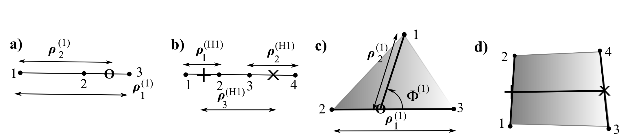
Figure 2: O, + and $\times$ denote COM(23), COM(12) and COM(34) respectively, where COM(ab) is the centre of mass of particles a and b. a) is 3-stop metroland and b) is 4-stop metroland in Jacobi H-coordinates. c) is triangleland. Here, I furthermore define $\Phi^{(\mbox{\scriptsize a})}$ as the ‘Swiss army knife’ angle $\mbox{arccos}\big{(}\mbox{\boldmath$\rho$}_{1}^{(\mbox{\scriptsize a})}\cdot\mbox{\boldmath$\rho$}_{3}^{(\mbox{\scriptsize a})}/\rho_{1}^{(\mbox{\scriptsize a})}\rho_{3}^{(\mbox{\scriptsize a})}\big{)}$. d) I provide the 4 particles in the plane layout to make clear what I mean by H-coordinates: these are shaped like the strokes in the letter H, which is then ‘squashed’ in the 1-$d$ case. The figures’ other labels pick out which clustering each coordinate system is with respect to; these are dropped in subsequent computations.

The 1-$d$ pure-shape r-configuration spaces are [21] $\mathbb{S}^{N-2}$ and suitable shape variables are here the (ultra)spherical angles $\Theta^{\bar{\tt r}}$ [30], interpreted as functions of ratios of relative separations. E.g. for 4-stop metroland (a universe model consisting of 4 particles on a line), these are $\theta=\mbox{arctan}\big{(}\sqrt{\rho_{1}\mbox{}^{2}+\rho_{2}\mbox{}^{2}}/\rho_{3}\big{)}$ and $\phi=\mbox{arctan}(\rho_{2}/\rho_{1})$. The shape momenta are then [30, 14, 37]

$${\cal D}_{\phi}:=p_{\phi}=\mbox{n}_{1}\mbox{p}_{2}-\mbox{n}_{2}\mbox{p}_{1}={\mbox{\tt D}}_{2}\mbox{n}_{1}/\mbox{n}_{2}-{\mbox{\tt D}}_{1}\mbox{n}_{2}/\mbox{n}_{1}\mbox{ and }\mbox{ }{\cal D}_{\theta}:=p_{\theta}\mbox{ }.$$ (46)

The 2 -$d$ pure-shape r-configuration spaces are [98, 24] $\mathbb{CP}^{N-2}$ and suitable shape variables are here the inhomogenous coordinates ${\mbox{Z}}^{\bar{\tt r}}$. To interpret these complex coordinates in terms of the $N$-a-gons, it is useful to pass to their polar forms, ${\mbox{Z}}^{\bar{\tt r}}={\cal R}^{\bar{\tt r}}\mbox{exp}(i\Phi^{\bar{\tt r}})$. Then the moduli are, again, ratios of relative separations, and the phases are now relative angles. In the specific case of the scalefree triangle, there is one of each, e.g. in coordinates based around the {1,23} clustering, these are [23] $\Theta=2\,\mbox{arctan}(\rho_{2}/\rho_{1})$ and $\Phi=\mbox{arccos}\big{(}\mbox{\boldmath$\rho$}_{1}\cdot\mbox{\boldmath$\rho$}_{3}/\rho_{1}\rho_{3}\big{)}$ as per Fig 2d). The shape momenta for the $N$-a-gon are [14, 37]

$${\cal P}^{{\cal R}}_{\bar{\tt p}}=\left\{\frac{\delta_{\bar{\tt p}\bar{\tt q}}}{1+||{\cal R}||^{2}}-\frac{{\cal R}_{\bar{\tt p}}{\cal R}_{\bar{\tt q}}}{\{1+||{\cal R}||^{2}\}^{2}}\right\}{\cal R}_{\bar{\tt q}}^{*}\mbox{ }\mbox{ },\mbox{ }\mbox{ }{\cal P}^{\Theta}_{\widetilde{\mbox{\scriptsize p}}}=\left\{\frac{\delta_{\overline{\mbox{\scriptsize p}}\overline{\mbox{\scriptsize q}}}}{1+||{\cal R}||^{2}}-\frac{{\cal R}_{\overline{\mbox{\scriptsize p}}}{\cal R}_{\overline{\mbox{\scriptsize q}}}}{\{1+||{\cal R}||^{2}\}^{2}}\right\}{\cal R}_{\overline{\mbox{\scriptsize p}}}{\cal R}_{\overline{\mbox{\scriptsize q}}}\Theta_{\widetilde{\mbox{\scriptsize p}}}^{*}\mbox{ }.$$ (47)

The scalefree triangle subcase [23, 14, 37] can furthermore be expressed in terms of ${\cal D}_{\triangle}=:p_{\Theta}:=\Theta^{*}$, ${\cal J}=:p_{\Phi}:=\mbox{sin}^{2}\Theta\,\Phi^{*}$. Here, and more generally, I use ${\cal J}$ to denote angular momenta. This ${\cal J}$, moreover, clearly cannot be an overall angular momentum since $\mbox{\tt L}=0$ applies. It is indeed a relative angular momentum [28]:

$${\cal J}=I_{1}I_{2}\Phi^{*}/I=I_{1}I_{2}\{\theta_{2}^{*}-\theta_{1}^{*}\}/I=\{I_{1}\mbox{L}_{2}-I_{2}\mbox{L}_{1}\}/I=\mbox{L}_{2}=-\mbox{L}_{1}=\{\mbox{L}_{2}-\mbox{L}_{1}\}/2\mbox{ }.$$ (48)

Thus it can be interpreted as the angular momentum of one of the two constituent subsystems, minus the angular momentum of the other, or half of the difference between the two subsystems’ angular momenta. That this is indeed a relative angular momentum is also clear from it being the conjugate of a relative angle.

For scaled RPM’s, the shape-scale split [25] allows for one just to add a ‘radial’ scale variable to the above sets (though there are other presentations too, see below). In the polar form that makes the split manifest, they are as for the pure-shape case alongside scale $\rho$ (the hyperradius [99] which is the square root of the moment of inertia) and the momentum conjugate to this, $p_{\rho}=\rho^{*}$. For the triangle, one needs $I=\rho^{2}$ to place the angular part into standard spherical form. In the Cartesian form for $N$-stop metroland, one has $\rho^{i}$ coordinates with conjugate momenta $p_{i}=\rho_{j}^{*}$. The triangle also admits a Cartesian form: in terms of Dragt-type coordinates [102, 31],

$$\mbox{Dra}_{1}=2\,\mbox{\boldmath$\rho$}_{1}\cdot\mbox{\boldmath$\rho$}_{2}\mbox{ },\mbox{ }\mbox{ }\mbox{Dra}_{2}=2|\mbox{\boldmath$\rho$}_{1}\mbox{\scriptsize{\bf$\mbox{ }\times\mbox{ }$}}\mbox{\boldmath$\rho$}_{2}|_{3}\mbox{ },\mbox{ }\mbox{ }\mbox{Dra}_{3}=\mbox{\boldmath$\rho$}_{1}^{2}-\mbox{\boldmath$\rho$}_{2}^{2}\mbox{ }.$$ (49)

These coordinates can be interpreted [31] as a measure of anisoscelesness aniso, 4 $\times$ the mass-weighted area per unit moment of inertia of the triangle, and the ellipticity ellip of the base relative to the median (see [31] for more detail). Their conjugates are [14, 37]

$$\Pi^{\mbox{\scriptsize D}\mbox{\scriptsize r}\mbox{\scriptsize a}}_{\Gamma}=\mbox{Dra}_{\Gamma}^{*}\mbox{ }$$ (50)

(for $\Gamma$ taking values 1 to 3) which are rates of change of ellipticity (pure-dilational), area and anisoscelesness (these last two are part-dilational and part-rotational).

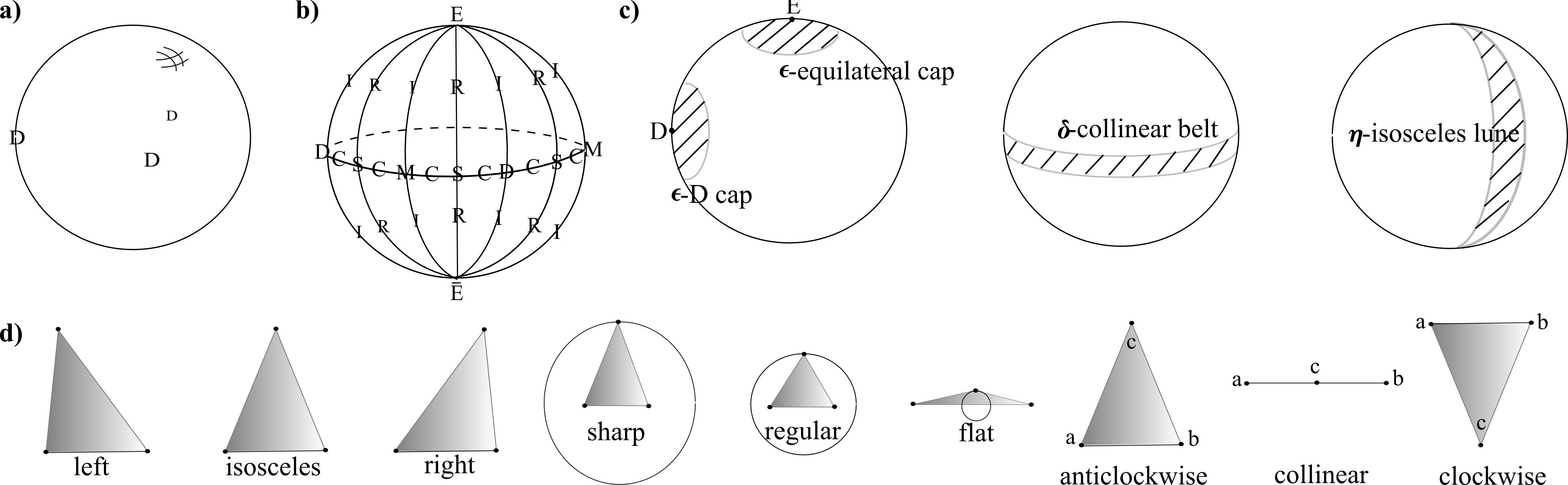
Figure 3: a) Triangleland at the topological level. b) Triangleland at the metric level. The [ ] basis has E as principal axis and D as second axis. On the other hand, the ( ) basis has D as principal axis and E as second axis. c) Some cap, belt and lune regions with particular physical significance [31] are as follows. The caps are of radius $\epsilon$, the belts of width $\delta$ and the lunes are of polar angular width $\eta$. The above are for pure-shape triangles; the scaled counterparts are in each case just the cones over the pure-shape cases. d) The nomenclature I use for dynamically convenient types of triangle. The most physically meaningful great circles on the triangleland shape correspond to the isosceles, regular and collinear triangles. These respectively divide the shape sphere into hemispheres of right and left triangles, sharp and flat triangles, and anticlockwise and clockwise triangles.

I give more detail of triangleland here, since scaled triangleland is the specific example that this paper makes use of. The configuration space for this in the case of distinguishable particles and in the plain shape case is the sphere, decorated as in Figs 3b) and 3f). The labelled points and edges have the following geometrical/mechanical interpretations. E and $\bar{\mbox{E}}$ are the two mirror images of labelled equilateral triangles. C are arcs of the equator that is made up of collinear configurations. This splits the triangleland shape sphere into two hemispheres of opposite orientation (clockwise and anticlockwise labelled triangles, as in Fig 3c). The I are bimeridians of isoscelesness with respect to the 3 possible clusterings (i.e. choices of base pair and apex particle). Each of these separates the triangleland shape sphere into hemispheres of right and left slanting triangles with respect to that choice of clustering [Fig 3c)]. The R are bimeridians of regularness (equality of the 2 partial moments of inertia of the each of the possible 2 constituent subsystems: base pair and apex particle.) Each of these separated the triangleland shape sphere into hemispheres of sharp and flat triangles with respect to that choice of clustering [Fig 3d)]. The M are merger points: where one particle lies at the centre of mass of the other two. S denotes spurious points, which lie at the intersection of R and C but have no further notable properties (unlike the D, M or E points that lie on the other intersections).

It is sometimes also convenient to swap the Dra₂ for the scale variable $I$ in the non-normalized version of the coordinates to obtain the {$I$, Dra₁, Dra₃} system. Then a simple linear recombination of this is {$I_{1}$, $I_{2}$, Dra₁}, i.e. the two partial moments of inertia and the anisoscelesness. This is in turn closely related [28] to the parabolic coordinates on the flat $\mathbb{R}^{3}$ conformal to the triangleland relational space, which are $\{I_{1},I_{2},\Phi\}$.

A physical interpretation for these is that $I_{1}$, $I_{2}$ are the partial moments of inertia of the base and the median, with $\Phi$ the ‘Swiss army knife’ angle between these (c.f. Fig 2) . They are clearly a sort of subsystem-split coordinates and thus useful in applications concerning subsystems [14, 38].

In each case, the quantum counterpart involves some operator form for the canonical variables and commutators in place of Poisson brackets. E.g. in the configuration representation the constituent operator variables are the shapes again, alongside differential operators for the shape momenta. In the case of the scaled triangle, these have the mathematics of the standard angular momentum operators albeit now with a more general interpretation as relative shape momenta (mixed relative-dilational and relative-angular momenta),

$$\mbox{sin}\,\Phi\,{\cal D}_{\triangle}+\mbox{cos}\,\Phi\,\mbox{cot}\,\Theta\,{\cal J}\mbox{ }\mbox{ and }\mbox{ }\mbox{ }-\mbox{cos}\,\Phi\,{\cal D}_{\triangle}+\mbox{sin}\,\Phi\,\mbox{cot}\,\Theta\,{\cal J}\mbox{ }.$$ (51)

There is the further issue use of conserved quantities in preference to/alongside the momenta.

1) These, or functions thereof, commute also with the Hamiltonian constraint and are thus Dirac beables. They manage this via not encountering an obstruction from the potential in the bracket of O and $H$.

2) They feature in the kinematical quantization procedure, making them even more natural at the quantum level. For the sphere, these are the $SU(2)$ quantities ${\cal S}_{i}$. Here also e.g. for the sphere, $\Phi$ and $\Theta$ are not good operators, it is, rather, the unit Cartesian vectors whose squares sum up to 1 that are. In total, one has ${\cal S}_{i}$, Dra^Γ and $\Pi^{\mbox{\scriptsize D}\mbox{\scriptsize r}\mbox{\scriptsize a}}_{\Gamma}$, forming the algebra

Eucl(3) $\mbox{Ⓢ}\mathbb{R}^{3}$, for Eucl(3) the ‘Euclidean group’ of translations and rotations (of 3-$d$ reduced configuration space) and where Ⓢ denotes semi-direct product.

The next simplest example concerns shape quantities and theory conjugate momenta for the quadrilateral and is presented in [36, 37], which are built on the kinematical considerations of [35]

As regards higher-$d$ RPM’s Kuchař observables, firstly I emphasize that these models are not needed to toy-model geometrodynamics [14]. Secondly, here the Best Matching Problem has a global obstruction to solvability – one can only invert the higher-$d$ inertia tensor present in the ${\cal L}$-constraint if one excludes the collinear configurations. And yet, these configurations are entirely physical so this localness of procedure is phys unsatisfactory. See Appendix 3.E of [14] for further detail of this second point.

4.2 Dirac observables solved for: Strategy 2 resolved

If one instead adheres to needing the more restrictive subset of complete observables, then one is to ask which functions of shape and shape momentum commute with the pure-shape RPM quadratic energy constraint, and which functions of scale, shape, scale momentum and shape momentum commute with the scaled RPM quadratic energy constraint.

A simple partial answer is that in a few cases these include (subsets) of the isometries, i.e. relative angular momenta, relative dilational momenta and linear combinations of these with certain shape-valued coefficients. E.g. this is a direct analogue of the angular momenta forming a complete set of commuting operators with the Hamiltonian operator, provided that the potential is central i.e. itself respecting the isometries of the sphere by being purely radial. Thus for the tower of $SO(p)$-symmetric problems (2 $\leq p\leq n$) for $N$-stop metrolands and triangleland, and its more elaborate counterpart for quadrilateralland in [37], we have found some complete observables. These are not, however, generically present i.e. for arbitrary-potential models. Another answer, at least in some simple models is that Halliwell’s class operators comply with ${\cal Q}\mbox{uad}$. For at least some simple $\mathfrak{g}$-trivial theories, Halliwell’s class operators are Dirac observables, and they or their phase space generalization may provide the complete set of such. See the next 3 Secs for more about this.

5 One way to extend Halliwell’s work to constrained theories

5.1 Nature of the extensions

Extension 1) I consider the case of linearly-constrained theories that are at least formally reducible. My treatment here

is purely quadratic/bosonic for simplicity. K is a coordinate vector for configurational Kuchař beables; these are independent and there are the right number $r$ = dim($\mbox{\Large$\mathfrak{q}$}^{\mbox{\scriptsize r}}$) of them to span. The complete set of Kuchař beables are more general: functionals $F[\mbox{{\bf K}},\mbox{\boldmath$\Pi$}^{\mbox{\tiny K}}]$. Having Kuchař beables explicitly available has close ties with one’s model being reducible; both are in practise exceptional circumstances. They do however apply to 1- and 2-$d$ RPM’s, which are indeed both reducible and have full sets of Kuchař beables known (c.f. Sec 6’s example). We present an alternative strategy in Sec 7 which, whilst indirect, is more widely applicable in cases without reducibility or knowledge of an explicit directly-expressed set of Kuchař beables. Full use of Kuchař beables would involve the extension of Halliwell’s construct to such as phase space regions since these are general functionals of Q, and P rather than just of Q.

Additionally, I consider a relational whole-universe context for which the following are held to apply.

Extension 2) Emergent time $t^{\mbox{\scriptsize e}\mbox{\scriptsize m}}$ emerges to fill in the role of $t$; this emergent time is the coincidence of [22] Jacobi–Barbour–Bertotti time [16, 17] at the classical level and WKB time at the semiclassical level [52].

Extension 3) Parageodesic principle conformal transformation (PPCT) invariance is held to apply by Misner’s argument [43] for conformal invariance as the second selector within DeWitt’s family of configuration space recoordinatization-invariant operator orderings [42] being grounded in the classical relational whole-universe models’ action [41, 14] being held to continue to apply at the quantum level. This involves the relational action (12) being manifestly invariant under the internal conformal invariance

$$\textrm{d}s_{\mbox{\scriptsize r}}^{2}\rightarrow\textrm{d}\overline{s}^{2}=\Omega^{2}\textrm{d}s_{\mbox{\scriptsize r}}^{2}\mbox{ },\mbox{ }\mbox{ }E-V\rightarrow\{\overline{E}-\overline{V}\}=\{E-V\}/\Omega^{2}\mbox{ }$$ (52)

(my notation here restricting to the reduced subcase, but this also applying to the minisuperspace GR setting of Misner). I next note that this implies the inverse of the configuration space metric to scale as

$$N_{\mbox{{\scriptsize A}}\mbox{{\scriptsize B}}}\rightarrow\overline{N}_{\mbox{{\scriptsize A}}\mbox{{\scriptsize B}}}=\Omega^{-2}N_{\mbox{{\scriptsize A}}\mbox{{\scriptsize B}}}$$ (53)

and the square-root of the determinant of the configuration space metric to scale as

$$\sqrt{|M|}\rightarrow\sqrt{|\overline{M}|}=\Omega^{r}\sqrt{|M|}\mbox{ }.$$ (54)

One next recovers Misner’s conformal covariance of the Hamiltonian constraint (or its generalization, ${\cal Q}$uad). Then taking this to carry over to the quantum level alongside DeWitt’s configuration space recoordinatization invariance implies that

i) the conformal operator ordering (which the preceding identifies as originating from specifically PPCT-invariance),

$$N^{\mbox{{\scriptsize A}}\mbox{{\scriptsize B}}}_{\mbox{\scriptsize r}}P^{\mbox{\scriptsize K}}_{\mbox{{\scriptsize A}}}P^{\mbox{\scriptsize K}}_{\mbox{{\scriptsize B}}}\mbox{ }\mbox{ }\stackrel{{\scriptstyle\mbox{\scriptsize promote to a quantum operator}}}{{\longrightarrow}}\mbox{ }\mbox{ }\triangle^{\mbox{\scriptsize c}}_{\mbox{\scriptsize r}}:=\triangle_{\mbox{\scriptsize r}}-\frac{r-2}{4\{r-1\}}\mbox{Ric}(M^{\mbox{\scriptsize r}})\mbox{ },$$ (55)

$$\mbox{for}\hskip 173.44756pt\triangle:=\frac{1}{\sqrt{M^{\mbox{\scriptsize r}}}}\frac{\partial}{\partial\mbox{K}^{\mbox{{\scriptsize A}}}}\left\{\sqrt{M^{\mbox{\scriptsize r}}}N_{\mbox{\scriptsize r}}^{\mbox{{\scriptsize A}}\mbox{{\scriptsize B}}}\frac{\partial}{\partial\mbox{K}^{\mbox{{\scriptsize B}}}}\right\}\hskip 238.49121pt$$ (56)

the usual Laplacian corresponding to $M^{\mbox{\scriptsize r}}_{\mbox{{\scriptsize A}}\mbox{{\scriptsize B}}}$.

ii) The wavefunctions are also then to scale as (see e.g. [103])

$$\Psi\longrightarrow\overline{\Psi}=\Omega^{\{2-r\}/2}\Psi\mbox{ }.$$ (57)

iii) For the physical quantities to be invariant, the corresponding inner product needs a weight function $\omega$ PPCT-scaling as

$$\omega\longrightarrow\overline{\omega}=\Omega^{-2}\omega$$ (58)

(see e.g. [29]), so that, by use of (54, 57, 58)

$$\int\overline{\mathbb{D}\mbox{{\bf K}}\,\Psi_{1}^{*}\Psi_{2}\omega}=\int\mathbb{D}\mbox{{\bf K}}\Omega^{r}\,\Psi_{1}^{*}\Psi_{2}\Omega^{2\{2-r\}/2}\omega\Omega^{-2}=\int\mathbb{D}\mbox{{\bf K}}\,\Psi_{1}^{*}\Psi_{2}\omega\mbox{ }.$$ (59)

Note that having explicit Kuchař observables implies reducibility, so that there is then no formal barrier to performing the above PPCT-invariant interpretation of conformally-invariant ordering. This matters insofar as conformally-invariant ordering does not in general commute with applying linear constraints [14], thus jeopardizing the argument for this ordering in all those case in which one cannot explicitly reduce first.

iv) Another ready corollary of (52) [41] is that the emergent time element scales as

$$\textrm{d}t^{\mbox{\scriptsize e}\mbox{\scriptsize m}}\longrightarrow\textrm{d}\overline{t}^{\mbox{\scriptsize e}\mbox{\scriptsize m}}=\Omega^{2}\textrm{d}t^{\mbox{\scriptsize e}\mbox{\scriptsize m}}\mbox{ }.$$ (60)

It then follows as a new result of this paper that $f_{\mbox{\scriptsize R}}$ needs to scale as $\Omega^{-2}$ so that the overall combination $\textrm{d}tf_{\mbox{\scriptsize R}}$ is PPCT-invariant. The below are also all new to this paper.

v) If one applies a PPCT to an $r$-manifold with metric $M_{\mbox{{\scriptsize a}}\mbox{{\scriptsize b}}}$ containing an {$r$ – 1}-dimensional hypersurface with metric $m_{\mbox{{\scriptsize a}}\mbox{{\scriptsize b}}}$ and normal $n^{\mbox{{\scriptsize a}}}_{\mbox{\scriptsize K}}$, then the formula for the induced metric implies that

$$m_{\mbox{{\scriptsize a}}\mbox{{\scriptsize b}}}\longrightarrow\overline{m}_{\mbox{{\scriptsize a}}\mbox{{\scriptsize b}}}=\Omega^{2}m_{\mbox{{\scriptsize a}}\mbox{{\scriptsize b}}}\mbox{ }\mbox{ and }\mbox{ }n_{\mbox{\scriptsize K}\mbox{{\scriptsize a}}}\longrightarrow\overline{n}_{\mbox{\scriptsize K}\mbox{{\scriptsize a}}}=\Omega n_{\mbox{\scriptsize K}\mbox{{\scriptsize a}}}$$ (61)

from which it immediately follows that

$$\sqrt{|m|}\longrightarrow\overline{\sqrt{|m|}}=\Omega^{r-1}\sqrt{m}\mbox{ }\mbox{ and }\mbox{ }n_{\mbox{\scriptsize K}}^{\mbox{{\scriptsize a}}}\longrightarrow\overline{n}_{\mbox{\scriptsize K}}^{\mbox{{\scriptsize a}}}=\Omega^{-1}n_{\mbox{\scriptsize K}}^{\mbox{{\scriptsize a}}}\mbox{ }.$$ (62)

vi) If (57) applies to a wavefunction obeying the BO-WKB ansätze form (6, 7), then preservation of the physically-significant h–l split under PPCT transformations requires it to be entirely the $\chi($h,l$)$ factor that PPCT-scales,

$$\chi\longrightarrow\overline{\chi}=\Omega^{\{2-r\}/2}\chi$$ (63)

since $\Omega$ itself is in general a function of h and l, and so would map $S$(h) out of the functions of h alone. Likewise it is the inner product integrating over the l-coordinates that carries a $\Omega^{-2}$ factor.

vii) The outer rather than inner product of two wavefunctions necessitates the same weight function; this will of course be used to build density matrices.

viii) The phase space measure does not PPCT-scale, as a result of the momentum space measure scaling oppositely to the configuration space one.

ix) Finally, I posit that the classical probability density w is PPCT-invariant, so that $\int\mathbb{D}\mbox{{\bf K}}\,\mathbb{D}\mbox{\boldmath$\Pi$}^{\mbox{\scriptsize K}}\mbox{w}(\mbox{{\bf K}},\mbox{\boldmath$\Pi$}^{\mbox{\scriptsize K}})$ is also.

5.2 Classical preliminary

Parallelling Halliwell, I begin by considering probability distributions, firstly on classical phase space, $\mbox{w}(\mbox{{\bf K}},\mbox{\boldmath$\Pi$}^{\mbox{\scriptsize K}})$ and then at the semiclassical level. For the classical analogue of energy eigenstate,

$$0=\frac{\partial\mbox{w}}{\partial t^{\mbox{\scriptsize e}\mbox{\scriptsize m}}}=\{H,\mbox{w}\}\mbox{ },$$ (64)

so w is constant along the classical orbits. I evoke $f_{\mbox{\scriptsize R}}(\mbox{{\bf q}})$ as the characteristic function of the region R, and makes use of a phase space function $A$ that is now not just any $A$ but an $A$ based on Kuchař observables K:

$$A(\mbox{{\bf K}},\mbox{{\bf K}}_{0},\mbox{\boldmath$\Pi$}^{\mbox{\scriptsize K}}_{0})=\int_{-\infty}^{+\infty}\textrm{d}t^{\mbox{\scriptsize e}\mbox{\scriptsize m}}\delta^{(r)}(\mbox{{\bf K}}-\mbox{{\bf K}}^{\mbox{\scriptsize c}\mbox{\scriptsize l}}(t^{\mbox{\scriptsize e}\mbox{\scriptsize m}}))\mbox{ }.$$ (65)

$$\mbox{Then}\hskip 130.08621pt\{{\cal L}\mbox{i}\mbox{n},A(\mbox{{\bf K}},\mbox{{\bf K}}_{0},\mbox{\boldmath$\Pi$}^{\mbox{\scriptsize K}}_{0})\}=\int_{-\infty}^{+\infty}\textrm{d}t^{\mbox{\scriptsize e}\mbox{\scriptsize m}}\{{\cal L}\mbox{i}\mbox{n},\delta^{(r)}(\mbox{{\bf K}}-\mbox{{\bf K}}^{\mbox{\scriptsize c}\mbox{\scriptsize l}}(t^{\mbox{\scriptsize e}\mbox{\scriptsize m}}))\}\mbox{ },\hskip 158.99377pt$$ (66)

$$\mbox{and}\hskip 227.65005pt\{{\cal L}\mbox{i}\mbox{n},\mbox{{\bf K}}\}=0\hskip 245.71754pt$$ (67)

because the K are Kuchař, so $\{{\cal L}\mbox{i}\mbox{n},f(\mbox{{\bf K}})\}=0$ by the chain-rule, and so

$$\{{\cal L}\mbox{i}\mbox{n},A(\mbox{{\bf K}},\mbox{{\bf K}}_{0},\mbox{\boldmath$\Pi$}^{\mbox{\scriptsize K}}_{0})\}=0\mbox{ }.$$ (68)

Moreover, being in terms of a vector of Kuchař observables does not change the argument by which

$$\{{\cal Q}\mbox{u}\mbox{a}\mbox{d},A(\mbox{{\bf K}},\mbox{{\bf K}}_{0},\mbox{\boldmath$\Pi$}^{\mbox{\scriptsize K}}_{0})\}=0$$ (69)

(which Halliwell has already demonstrated to be robust to curved configuration space use). Thus, by (68,69) combined,

1) (65) are Dirac.

2) As substantial a set of Dirac observables can be built thus for a theory whose full set of Kuchař observables are known as could be built for Halliwell’s simpler non linearly-constrained theories. To that extent, one has a formal construction of the Unicorn. [Though, at the QM level, this role of A is played out again by the class operators instead.]

Moreover, in the case of 1- and 2-$d$ RPM’s, scaled or unscaled, Sec 4 ensures that this is an actual construction for these toy models’ toy Unicorn.

$$\mbox{Next,}\hskip 36.135pt\mbox{Prob(intersection with R)}=\int_{-\infty}^{+\infty}\textrm{d}t^{\mbox{\scriptsize e}\mbox{\scriptsize m}}\,f_{\mbox{\scriptsize R}}(\mbox{\bf K}^{\mbox{\scriptsize c}\mbox{\scriptsize l}}(t^{\mbox{\scriptsize e}\mbox{\scriptsize m}}))=\int\mathbb{D}\mbox{\bf K}\,f_{\mbox{\scriptsize R}}(\mbox{{\bf q}})\,\int_{-\infty}^{+\infty}\textrm{d}t^{\mbox{\scriptsize e}\mbox{\scriptsize m}}\delta^{(r)}\big{(}\mbox{\bf K}-\mbox{\bf K}^{\mbox{\scriptsize c}\mbox{\scriptsize l}}(t^{\mbox{\scriptsize e}\mbox{\scriptsize m}})\big{)}\hskip 289.07999pt$$

$$=\int\mathbb{D}\mbox{\bf K}\,f_{\mbox{\scriptsize R}}(\mbox{{\bf K}})\,A(\mbox{\bf K},\mbox{\bf K}_{0},\mbox{\boldmath$\Pi$}^{\mbox{\scriptsize K}}_{0}):$$ (70)

the ‘amount of $t^{\mbox{\scriptsize e}\mbox{\scriptsize m}}$’ the trajectory spends in R; moreover this physical quantity is constructed to be PPCT-invariant by iv).

$$\mbox{Then,}\hskip 86.72377ptP_{\mbox{\scriptsize R}}=\int\mathbb{D}\mbox{\boldmath$\Pi$}^{\mbox{\scriptsize K}}_{0}\,\mathbb{D}\mbox{\bf K}_{0}\,\mbox{w}\big{(}\mbox{\bf K}_{0},\mbox{\boldmath$\Pi$}^{\mbox{\scriptsize K}}_{0}\big{)}\,\,\theta\left(\int_{-\infty}^{+\infty}\textrm{d}t^{\mbox{\scriptsize e}\mbox{\scriptsize m}}f_{\mbox{\scriptsize R}}\big{(}\mbox{\bf K}^{\mbox{\scriptsize c}\mbox{\scriptsize l}}(t^{\mbox{\scriptsize e}\mbox{\scriptsize m}})\big{)}-\epsilon\right)\mbox{ },\hskip 289.07999pt$$ (71)

which is PPCT-invariant through coming in three factors each of which is PPCT-invariant [by viii) and ix)].

Note that the window function corresponding to the region R is assumed to fit on a single coordinate system, limiting it to being somewhat local. This is entirely fine if one is considering small regions (see Sec 6 for more). This also continues to work approximately for compact RCS’s like pure-shape RPM examples have (c.f. Fig 3).

An alternative expression is for the flux through a piece of an {$r$ – 1}-$d$ hypersurface within the configuration space,

$$P_{\Sigma}=\int\textrm{d}t^{\mbox{\scriptsize e}\mbox{\scriptsize m}}\int\int\mathbb{D}\mbox{\boldmath$\Pi$}^{\mbox{\scriptsize K}}_{0}\,\mathbb{D}\mbox{\bf K}_{0}\,\mbox{w}(\mbox{\bf K}_{0},\mbox{\boldmath$\Pi$}^{\mbox{\scriptsize K}}_{0})\int_{\Sigma}\textrm{d}^{2}{\Sigma}(\mbox{\bf K}^{\prime})\,\mbox{\bf n}^{\mbox{\scriptsize K}\prime}\cdot\frac{\textrm{d}\mbox{\bf K}^{\mbox{\scriptsize c}\mbox{\scriptsize l}}(t^{\mbox{\scriptsize e}\mbox{\scriptsize m}})}{\textrm{d}t^{\mbox{\scriptsize e}\mbox{\scriptsize m}}}\,\delta^{(r)}\big{(}\mbox{\bf K}-\mbox{\bf K}^{\mbox{\scriptsize c}\mbox{\scriptsize l}}(t^{\mbox{\scriptsize e}\mbox{\scriptsize m}})\big{)}$$

$$=\int\textrm{d}t^{\mbox{\scriptsize e}\mbox{\scriptsize m}}\int\mathbb{D}\mbox{\boldmath$\Pi$}^{\mbox{\scriptsize K}\prime}\int_{\Sigma}\mathbb{D}{\Sigma}(\mbox{\bf K}^{\prime})\,\mbox{\bf n}^{\mbox{\scriptsize K}\prime}\cdot\mbox{\boldmath$\Pi$}^{\mbox{\scriptsize K}\prime}\,\mbox{w}(\mbox{\bf K}^{\prime},\mbox{\boldmath$\Pi$}^{\mbox{\scriptsize K}})\mbox{ },$$ (72)

the latter equality being by passing to $\mbox{\bf K}^{\prime}:=\mbox{\bf K}^{\mbox{\scriptsize c}\mbox{\scriptsize l}}(t^{\mbox{\scriptsize e}\mbox{\scriptsize m}})$ and $\mbox{\boldmath$\Pi$}^{\mbox{\scriptsize K}}:=\mbox{\boldmath$\Pi$}^{\mbox{\scriptsize K}}_{\mbox{\scriptsize c}\mbox{\scriptsize l}}(t^{\mbox{\scriptsize e}\mbox{\scriptsize m}})$ coordinates at each $t^{\mbox{\scriptsize e}\mbox{\scriptsize m}}$. This is again PPCT-invariant, by v), viii) and ix).

5.3 Semiclassical quantum working

Extension 4): Wigner function in curved space. As well as previous considerations of volume elements, this has the further subtlety that the sums inside the bra and ket are no longer trivially defined. This was resolved by Winter, Calzetta, Habib, Hu and Kandrup [104], by Fonarev [105] and by Liu and Qian [106] in the case of Riemannian configuration space geometry via local geodesic constructions.

Underhill’s earlier study [107] works with just affine structure assumed. (In searching for this topic in the literature, it is useful to note that the Wigner function is closely related to the Weyl transformation; see also Sec 2.3 of the review [108].) Liu and Qian also extended their work [106] to principal bundles over Riemannian manifolds, thus covering what is required to extend Sec 7 in terms of Wigner functions. Because of this, I specifically take ‘Wigner functions in curved space’ in the sense of Liu and Qian when in need of sufficiently detailed considerations. Finally, I emphasize again that Wigner functions are only temporary passengers in the present program due to their being used in Halliwell 2003 types implementations of class operators but no longer in Halliwell 2009 ones, by which I keep the account of this SSec’s subtleties brief.

The preceding alternative expression has further parallel with the Wigner function at the semiclassical level. Next, [91]’s straightforward approximations in deriving (32) locally carry over, so

$$\mbox{Wig}(\mbox{\bf K},\mbox{\boldmath$\Pi$}^{\mbox{\scriptsize K}})\approx|\chi(\mbox{\bf K})|^{2}\delta^{(r)}(\mbox{\boldmath$\Pi$}^{\mbox{\scriptsize K}}-{\mbox{\boldmath{$\nabla$}}}^{\mbox{\scriptsize K}}S)$$ (73)

($\mbox{\boldmath$\Pi$}^{\mbox{\scriptsize K}}$ being ${\mbox{\boldmath{$\nabla$}}}^{\mbox{\scriptsize K}}S$ for classical trajectories). Then Halliwell’-type heuristic move is then to replace $w$ by Wig in (89), giving

$$P_{\Sigma}^{\mbox{\scriptsize s}\mbox{\scriptsize e}\mbox{\scriptsize m}\mbox{\scriptsize i}\mbox{\scriptsize c}\mbox{\scriptsize l}}\approx\int\textrm{d}t^{\mbox{\scriptsize e}\mbox{\scriptsize m}}\int_{\Sigma}\textrm{d}\Sigma(\mbox{{\bf K}})\mbox{\bf n}^{\mbox{\scriptsize K}}\frac{\nabla S}{\nabla\mbox{\bf K}}|\chi(\mbox{\bf K})|^{2}\mbox{ }.$$ (74)

This remains PPCT-invariant as the quantum inner product and the classical $\int\textrm{d}\mbox{\boldmath$\Pi$}^{\mbox{\scriptsize K}}\mbox{w}(\mbox{{\bf K}},\mbox{\boldmath$\Pi$}^{\mbox{\scriptsize K}})$ both scale equally as $\Omega^{-r}$.

5.4 Class operators

The Halliwell-type treatment continues within the framework of decoherent histories, which I take as formally standard for this setting too. The key step for this continuation is the construction of class operators, which uplifts a number of features of the preceding structures. One now uses

$${C}^{\sharp}_{\mbox{\scriptsize R}}=\theta\left(\int_{-\infty}^{+\infty}\textrm{d}tf_{\mbox{\scriptsize R}}(\mbox{{\bf K}}(t))-\epsilon\right)P(\mbox{{\bf K}}_{\mbox{\scriptsize f}},\mbox{{\bf K}}_{0})\,\mbox{exp}(iA(\mbox{{\bf K}}_{\mbox{\scriptsize f}},\mbox{{\bf K}}_{0}))\mbox{ },$$ (75)

which, by construction, obeys

$$|[{\cal Q}\mbox{uad},C^{\sharp}_{\mbox{\scriptsize R}}]|=0\mbox{ };$$ (76)

$$|[{\cal L}\mbox{in},C^{\sharp}_{\mbox{\scriptsize R}}]|=0$$ (77)

also holds as $C^{\sharp}_{\mbox{\scriptsize R}}$ is a functional of Kuchař beables. As the cofactor of $\theta$ is some approximand to the quantum wavefunction, it PPCT-scales as $\Omega^{\{2-r\}/2}$.

Again, this class operator is not the end of the story since it is technically unsatisfactory, as resolved in [67, 68] (and to be covered in Paper II), but the above form serves as a conceptual-and-technical start for RPM version of the work and extension to cases with linear constraints, and for the present conceptual, whole-universe and linear-constraint extending paper, this is as far as we shall go.

5.5 Decoherence functional

The decoherence functional is of the form

$$\mbox{Dec}(\alpha,\alpha^{\prime})=\int_{\alpha}\mathbb{D}\mbox{{\bf K}}\int_{\alpha^{\prime}}\mathbb{D}\mbox{{\bf K}}^{\prime}\mbox{exp}(i\{S[\mbox{{\bf K}}(t^{\mbox{\scriptsize e}\mbox{\scriptsize m}})]-S[\mbox{{\bf K}}^{\prime}(t^{\mbox{\scriptsize e}\mbox{\scriptsize m}})]\}\mbox{\Large$\rho$}(\mbox{{\bf K}}_{0},\mbox{{\bf K}}_{0}^{\prime})\omega_{\mbox{\scriptsize d}}\mbox{ }.$$ (78)

For this to be PPCT-invariant as befits a physical quantity, it needs to have its own weight $\omega_{\mbox{\scriptsize d}}$, PPCT-scaling as $\omega_{\mbox{\scriptsize d}}\longrightarrow\overline{\omega}_{\mbox{\scriptsize d}}=\Omega^{-r}\omega_{\mbox{\scriptsize d}}$. Class operators are then fed into the expression for the decoherence functional, giving

$$\mbox{Dec}(\alpha,\alpha^{\prime})=\int\int\int\textrm{d}^{3}\mbox{{\bf K}}_{\mbox{\scriptsize f}}\textrm{d}^{3}\mbox{{\bf K}}_{0}\textrm{d}^{3}\mbox{{\bf K}}^{\prime}_{\mbox{\scriptsize f}}C^{{\sharp}}_{\alpha}(\mbox{{\bf K}}_{\mbox{\scriptsize f}},\mbox{{\bf K}}_{0})C^{{\sharp}}_{\alpha^{\prime}}(\mbox{{\bf K}}^{\prime}_{\mbox{\scriptsize f}},\mbox{{\bf K}}^{\prime}_{0})\Psi(\mbox{{\bf K}}_{0})\Psi(\mbox{{\bf K}}^{\prime}_{0})\omega^{2}\omega_{\mbox{\scriptsize d}}\mbox{ }.$$ (79)

The $\omega^{2}$ factor has one $\omega$ arise from the density matrix and the other from the 2-wavefunction approximand expressions from the two $C^{\prime}$’s. If the universe contains a classically-negligible but QM-non-negligible environment as per Appendix A, the influence functional ${\cal F}$ makes conceptual sense and one can rearrange (79) in terms of this into the form

$$\mbox{Dec}(\alpha,\alpha^{\prime})=\int\int\int\mathbb{D}\mbox{{\bf K}}_{\mbox{\scriptsize f}}\mathbb{D}\mbox{{\bf K}}_{0}\mathbb{D}\mbox{{\bf K}}_{0}^{{}^{\prime}}C_{\alpha}^{\sharp}(\mbox{{\bf K}}_{\mbox{\scriptsize f}},\mbox{{\bf K}}_{0})C_{\alpha}^{\sharp}(\mbox{{\bf K}}_{\mbox{\scriptsize f}},\mbox{{\bf K}}_{0})^{{}^{\prime}}{\cal F}(\mbox{{\bf K}}_{\mbox{\scriptsize f}},\mbox{{\bf K}}_{0},\mbox{{\bf K}}_{0}^{{}^{\prime}})\Psi(\mbox{{\bf K}}_{0})\Psi^{*}(\mbox{{\bf K}}_{0}^{{}^{\prime}})\omega^{2}\omega_{\mbox{\scriptsize d}}\mbox{ }.$$ (80)

6 Example: r-presentation of triangleland

6.1 Classical counterpart

Regions of configuration space for RPM’s, includes cases of particularly lucid physical significance as per Sec 4’s tessellation interpretation. Now,

$$P_{\mbox{\scriptsize R}}:=\mbox{Prob}(\mbox{classical solution will pass through a triangleland configuration space region R})\mbox{ }.$$ (81)

Next, I evoke $f_{\mbox{\scriptsize R}}(\mbox{\bf Dra})$ as the characteristic function of the triangleland configuration space region R, and makes use of phase space functions

$$A(\mbox{\bf Dra},\mbox{\bf Dra}_{0},\mbox{\boldmath$\Pi$}^{\mbox{\scriptsize D}\mbox{\scriptsize r}\mbox{\scriptsize a}}_{0})=\int_{-\infty}^{+\infty}\textrm{d}t^{\mbox{\scriptsize e}\mbox{\scriptsize m}}\delta^{(3)}\big{(}\mbox{\bf Dra}-\mbox{\bf Dra}^{\mbox{\scriptsize c}\mbox{\scriptsize l}}(t^{\mbox{\scriptsize e}\mbox{\scriptsize m}})\big{)}\mbox{ }.$$ (82)

These commute with ${\cal L}$ and ${\cal E}$ by the argument around equations (66-69). Then

$$\mbox{Prob(intersection with R)}=\int_{-\infty}^{+\infty}\textrm{d}t^{\mbox{\scriptsize e}\mbox{\scriptsize m}}\,f_{\mbox{\scriptsize R}}(\mbox{\bf Dra}^{\mbox{\scriptsize c}\mbox{\scriptsize l}}(t^{\mbox{\scriptsize e}\mbox{\scriptsize m}}))=\int\mathbb{D}\mbox{\bf Dra}\,f_{\mbox{\scriptsize R}}(\mbox{{\bf q}})\,\int_{-\infty}^{+\infty}\textrm{d}t^{\mbox{\scriptsize e}\mbox{\scriptsize m}}\delta^{(k)}\big{(}\mbox{\bf Dra}-\mbox{\bf Dra}^{\mbox{\scriptsize c}\mbox{\scriptsize l}}(t^{\mbox{\scriptsize e}\mbox{\scriptsize m}})\big{)}$$

$$=\int\mathbb{D}\mbox{\bf Dra}\,f_{\mbox{\scriptsize R}}(\mbox{\bf Dra})\,A(\mbox{\bf Dra},\mbox{\bf Dra}_{0},\mbox{\boldmath$\Pi$}^{\mbox{\scriptsize D}\mbox{\scriptsize r}\mbox{\scriptsize a}}_{0})\mbox{ }:$$ (83)

the ‘amount of $t^{\mbox{\scriptsize e}\mbox{\scriptsize m}}$’ the trajectory spends in region R. Then

$$P_{\mbox{\scriptsize R}}=\int\textrm{d}^{3}\mbox{\boldmath$\Pi$}^{\mbox{\scriptsize D}\mbox{\scriptsize r}\mbox{\scriptsize a}}_{0}\,\textrm{d}^{3}\mbox{\bf Dra}_{0}\,\mbox{w}\big{(}\mbox{\bf Dra}_{0},\mbox{\boldmath$\Pi$}^{\mbox{\scriptsize D}\mbox{\scriptsize r}\mbox{\scriptsize a}}_{0}\big{)}\,\,\theta\left(\int_{-\infty}^{+\infty}\textrm{d}t^{\mbox{\scriptsize e}\mbox{\scriptsize m}}f_{\mbox{\scriptsize R}}\big{(}\mbox{\bf Dra}^{\mbox{\scriptsize c}\mbox{\scriptsize l}}(t^{\mbox{\scriptsize e}\mbox{\scriptsize m}})\big{)}-\epsilon\right)\mbox{ }.$$ (84)

Halliwell illustrated this with a free particle model; this has a counterpart for the r-presentation of the scaled triangle free classical solution via the Dragt correspondence of [25, 14] which amounts to transcribing Halliwell’s mathematics to an arena in which it has whole-universe significance.

An alternative expression is for the flux through a piece of a 2-$d$ hypersurface within the configuration space,

$$P_{\Sigma}=\int\textrm{d}t^{\mbox{\scriptsize e}\mbox{\scriptsize m}}\int\textrm{d}^{3}\mbox{\boldmath$\Pi$}^{\mbox{\scriptsize D}\mbox{\scriptsize r}\mbox{\scriptsize a}}_{0}\,\textrm{d}^{3}\mbox{\bf Dra}_{0}\,\mbox{w}(\mbox{\bf Dra}_{0},\mbox{\boldmath$\Pi$}^{\mbox{\scriptsize D}\mbox{\scriptsize r}\mbox{\scriptsize a}}_{0})\int_{\Sigma}\textrm{d}^{2}{\Sigma}(\mbox{\bf Dra})\,\mbox{\bf n}^{\mbox{\scriptsize D}\mbox{\scriptsize r}\mbox{\scriptsize a}}\cdot\mbox{{\bf M}}\cdot\frac{\textrm{d}\mbox{\bf Dra}^{\mbox{\scriptsize c}\mbox{\scriptsize l}}(t^{\mbox{\scriptsize e}\mbox{\scriptsize m}})}{\textrm{d}t^{\mbox{\scriptsize e}\mbox{\scriptsize m}}}\,\delta^{(k)}\big{(}\mbox{\bf Dra}-\mbox{\bf Dra}^{\mbox{\scriptsize c}\mbox{\scriptsize l}}(t^{\mbox{\scriptsize e}\mbox{\scriptsize m}})\big{)}$$

$$=\int\textrm{d}t^{\mbox{\scriptsize e}\mbox{\scriptsize m}}\int\mathbb{D}\mbox{\boldmath$\Pi$}^{\mbox{\scriptsize D}\mbox{\scriptsize r}\mbox{\scriptsize a}\prime}\int_{\Sigma}\mathbb{D}{\Sigma}(\mbox{\bf Dra}^{\prime})\,\mbox{\bf n}^{\mbox{\scriptsize D}\mbox{\scriptsize r}\mbox{\scriptsize a}\prime}\cdot\mbox{\boldmath$\Pi$}^{\mbox{\scriptsize D}\mbox{\scriptsize r}\mbox{\scriptsize a}\prime}\,\mbox{w}(\mbox{\bf Dra}^{\prime},\mbox{\boldmath$\Pi$}^{\mbox{\scriptsize D}\mbox{\scriptsize r}\mbox{\scriptsize a}\prime})\mbox{ },$$ (85)

the latter equality being by passing to $\mbox{\bf Dra}^{\prime}:=\mbox{\bf Dra}^{\mbox{\scriptsize c}\mbox{\scriptsize l}}(t^{\mbox{\scriptsize e}\mbox{\scriptsize m}})$ and $\mbox{\boldmath$\Pi$}^{\mbox{\scriptsize D}\mbox{\scriptsize r}\mbox{\scriptsize a}\prime}:=\mbox{\boldmath$\Pi$}^{\mbox{\scriptsize D}\mbox{\scriptsize r}\mbox{\scriptsize a}}_{\mbox{\scriptsize c}\mbox{\scriptsize l}}(t^{\mbox{\scriptsize e}\mbox{\scriptsize m}})$ coordinates at each $t^{\mbox{\scriptsize e}\mbox{\scriptsize m}}$.

6.2 Semiclassical quantum working

The last alternative above further parallel at the semiclassical level with the Wigner function. Now, including a power of the PPCT conformal factor,

$$\mbox{Wig}(\mbox{\boldmath$\Pi$}^{\mbox{\scriptsize D}\mbox{\scriptsize r}\mbox{\scriptsize a}},\mbox{\bf Dra})\approx|\chi(\mbox{\bf Dra})|^{2}\delta^{(3)}(\mbox{\boldmath$\Pi$}^{\mbox{\scriptsize D}\mbox{\scriptsize r}\mbox{\scriptsize a}}-{\mbox{\boldmath{$\nabla$}}}^{\mbox{\scriptsize D}\mbox{\scriptsize r}\mbox{\scriptsize a}}S)/\{4\mbox{I}\}^{3/2}\mbox{ }$$ (86)

($\mbox{\boldmath$\Pi$}^{\mbox{\scriptsize D}\mbox{\scriptsize r}\mbox{\scriptsize a}}={\mbox{\boldmath{$\nabla$}}}^{\mbox{\scriptsize D}\mbox{\scriptsize r}\mbox{\scriptsize a}}S$ for classical trajectories). I note that in my setting of interest, $|\chi\rangle=|\chi(\Theta,\Phi,\mbox{I})\rangle$ and $S=S(\mbox{I})$. Halliwell’s heuristic move is then to replace w by Wig in (89)

$$P_{\Sigma}^{\mbox{\scriptsize s}\mbox{\scriptsize e}\mbox{\scriptsize m}\mbox{\scriptsize i}\mbox{\scriptsize c}\mbox{\scriptsize l}}\approx\int\textrm{d}t^{\mbox{\scriptsize e}\mbox{\scriptsize m}}\int_{\Sigma}\mathbb{D}\Sigma(\mbox{Dra})\mbox{\bf n}^{\mbox{\scriptsize D}\mbox{\scriptsize r}\mbox{\scriptsize a}}\frac{\nabla S}{\nabla\mbox{\bf Dra}}|\chi(\mbox{\bf Dra})|^{2}\mbox{ }.$$ (87)

The RPM case of most interest is that with the radial ‘scale of the universe’ direction having particular h-significance, by which the configurational 2-surface element is a piece of sphere with a number of these carrying lucid significance by Sec 4 and the 3-momentum 3-surface element is the spherical polars one (modulo conformal factors). Moreover, the $S$ makes the evaluation of this in spherical polars natural, even if $\Sigma$ itself is unaligned with those (though it simplifies the calculation if

there is such an alignment).

So rewriting (87) in conformal–spherical polar coordinates, e.g. for

$$\mbox{\scriptsize Prob(universe attains size I${}_{0}$ $\pm\delta$I whilst being $\epsilon$-equilateral)}\approx\int_{t^{\mbox{\scriptsize e}\mbox{\scriptsize m}}=t_{0}-\delta t}^{t_{0}+\delta t}\textrm{d}t^{\mbox{\scriptsize e}\mbox{\scriptsize m}}\int_{\Phi=0}^{2\pi}\int_{\Theta=0}^{\epsilon}\mbox{I}^{2}\mbox{sin}\,\Theta\,\textrm{d}\,\Theta\textrm{d}\,\Phi\frac{\textrm{d}S(\mbox{I})}{\textrm{d}\mbox{I}}|\chi(\mbox{I},\Theta,\Phi)|^{2}\mbox{ }.$$ (88)

This made use of this question by addressed by the $\epsilon-cap$ about the E-pole, which is very simply parametrized by the coordinates in use [see Fig 3c) for this cap and the below belt]. Also, $S=S(\mbox{I})$ alone, so $\mbox{\bf n}^{\mbox{\scriptsize D}\mbox{\scriptsize r}\mbox{\scriptsize a}\prime}{\nabla S}/{\nabla\mbox{\bf Dra}^{\prime}}$ becomes a radial $\mbox{\bf n}^{\mbox{\scriptsize I}}\,\partial S/\partial\mbox{I}$ factor and two zero components. To proceed, $\textrm{d}t^{\mbox{\scriptsize e}\mbox{\scriptsize m}}\frac{\textrm{d}S}{\textrm{d}\mbox{\scriptsize I}}$ = $\textrm{d}t^{\mbox{\scriptsize e}\mbox{\scriptsize m}}\frac{\textrm{d}\mbox{\scriptsize I}}{\textrm{d}t^{\mbox{\scriptsize e}\mbox{\scriptsize m}}}=\textrm{d}\mbox{I}$ by the Hamilton–Jacobi expression for momentum, the momentum-velocity relation and the chain-rule, so we do not need to explicitly evaluate $t_{0}\pm\delta t$ in terms of $\mbox{I}\pm\delta I$. Then e.g. for the approximate semiclassical wavefunction from the explicit triangleland example in [34] (the upside-down harmonic oscillator for the universe at zero energy),

$$\mbox{\scriptsize{Prob(universe attains size I $\pm\delta$I whilst being $\epsilon$-equilateral)}}\approx 2\mbox{I}_{0}^{2}\delta\mbox{I}\int_{\Theta=0}^{\epsilon}\int_{\Phi=0}^{2\pi}|Y_{\mbox{\scriptsize S}\,\mbox{s}}(\Theta,\Phi)|^{2}\mbox{sin}\,\Theta\,\textrm{d}\Theta\,\textrm{d}\Phi+O(\delta\mbox{I}^{2})\mbox{ }.$$ (89)

Here, the $Y_{\mbox{\scriptsize S}\mbox{\scriptsize s}}$ are spherical harmonics indexed by triangleland’s total shape momentum in the [ ] basis defined in Fig 3’s caption. The answer then comes out with leading term proportional to e.g. $\mbox{I}_{0}^{2}\delta\mbox{I}\,\epsilon^{2}$ for all the axially-symmetric wavefuntions $\chi_{\mbox{\scriptsize S}\,0}\propto Y_{\mbox{\scriptsize S}\,0}$ and to $\mbox{I}_{0}^{2}\delta\mbox{I}\,\epsilon^{4}$ for the first non-axial wavefunctions (the sine and cosine combinations corresponding to the quantum numbers S and $|\mbox{s}|$ = 1). These answers make good sense as regards the axisymmetric wavefuntions being peaked around the equilateral triangle whilst the equilateral triangle is nodal for the first non-axisymmetric wavefunctions.

Note 1) This is an Naïve Schrödinger Interpretation-type construct, though it is for the semiclassical l-part, so there is some kind of semiclassical imprint left on it.

Note 2) Prob(universe attains size I $\pm\delta$I whilst being $\epsilon$-D) is given likewise but for a particular D being given by the same in the corresponding ( ) basis, and the words “one orientation” or “a particular D” being suppressible by summing over various such integrals.

Note 3) As a final example,

$$\mbox{\scriptsize Prob(universe attains size I $\pm\delta$I whilst being $\epsilon$-collinear)}\mbox{ }\mbox{ has $\epsilon$-cap replaced by $\epsilon$-belt about the equator in the [ ] basis}\mbox{ },$$ (90)

and the answer goes as as $\mbox{I}_{0}^{2}\delta\mbox{I}\,\epsilon^{3}$ for the odd-S axisymmetric wavefunctions and as $\mbox{I}_{0}^{2}\delta\mbox{I}\,\epsilon$ for the even-S axisymmetric wavefunctions and the first non-axisymmetric ones. This has one power of $\epsilon$ less than for the above example since cap area $\propto\epsilon^{2}$ but belt area $\propto\epsilon$ only. The extra $\epsilon^{2}$ factor can again be explained in terms of peaks and nodes: a nodal plane of collinearity as compared to peaks on all or part of it.

6.3 Class operators

Again, one uses the modified version, which here takes the form

$${C}_{\mbox{\scriptsize R}}^{\sharp}=\theta\left(\int_{-\infty}^{+\infty}\textrm{d}tf_{\mbox{\scriptsize R}}(\mbox{\bf Dra}(t^{\mbox{\scriptsize e}\mbox{\scriptsize m}}))-\epsilon\right)P(\mbox{\bf Dra}_{\mbox{\scriptsize f}},\mbox{\bf Dra}_{0})\,\mbox{exp}(iA(\mbox{\bf Dra}_{\mbox{\scriptsize f}},\mbox{\bf Dra}_{0}))\mbox{ }.$$ (91)

$$\mbox{This obeys}\hskip 151.76744pt|[{\cal E},C^{\sharp}]|=0\mbox{ },\mbox{ }\mbox{ }|[{\cal L},C^{\sharp}]|=0\mbox{ }.\hskip 180.67499pt$$ (92)

6.4 Decoherence functionals

Class operators are then fed into the expression for the decoherence functional,

$$\mbox{Dec}(\alpha,\alpha^{\prime})=\int_{\alpha}\textrm{d}^{3}\mbox{\bf Dra}\int_{\alpha^{\prime}}\textrm{d}^{3}\mbox{\bf Dra}^{\prime}\mbox{exp}(i\{S[\mbox{\bf Dra}(t^{\mbox{\scriptsize e}\mbox{\scriptsize m}})]-S[\mbox{\bf Dra}(t^{\mbox{\scriptsize e}\mbox{\scriptsize m}})])\}\mbox{\Large$\rho$}(\mbox{\bf Dra}_{\mbox{\scriptsize i}\mbox{\scriptsize n}},\mbox{\bf Dra}_{\mbox{\scriptsize i}\mbox{\scriptsize n}}^{\prime})\mbox{ },$$ (93)

$$\mbox{giving}\hskip 43.36243pt\mbox{Dec}(\alpha,\alpha^{\prime})=\int\int\int\textrm{d}^{3}\mbox{\bf Dra}_{\mbox{\scriptsize f}}\textrm{d}^{3}\mbox{\bf Dra}_{0}\textrm{d}^{3}\mbox{\bf Dra}^{\prime}_{\mbox{\scriptsize f}}\,{C}^{\sharp}_{\alpha}(\mbox{\bf Dra}_{\mbox{\scriptsize f}},\mbox{\bf Dra}_{0})\,{C}^{\sharp}_{\alpha^{\prime}}(\mbox{\bf Dra}^{\prime}_{\mbox{\scriptsize f}},\mbox{\bf Dra}^{\prime}_{0})\Psi(\mbox{\bf Dra}_{\mbox{\scriptsize i}\mbox{\scriptsize n}})\Psi(\mbox{\bf Dra}^{\prime}_{\mbox{\scriptsize i}\mbox{\scriptsize n}})\mbox{ }.\hskip 43.36243pt$$ (94)

Under classically insignificant, QM significant environment assumption under which the influence functional is justified,

$$\mbox{Dec}(\alpha,\alpha^{\prime})=\int\int\int\textrm{d}^{3}\mbox{\bf Dra}_{\mbox{\scriptsize f}}\textrm{d}^{3}\mbox{\bf Dra}_{0}\textrm{d}^{3}\mbox{\bf Dra}_{0}^{\prime}\,{C}^{\sharp}_{\alpha}(\mbox{\bf Dra}_{\mbox{\scriptsize f}},\mbox{\bf Dra}_{0})\,{C}^{\sharp}_{\alpha}(\mbox{\bf Dra}_{\mbox{\scriptsize f}},\mbox{\bf Dra}_{0}^{\prime}){\cal F}(\mbox{\bf Dra}_{\mbox{\scriptsize f}},\mbox{\bf Dra}_{0},\mbox{\bf Dra}_{0}^{\prime})\Psi(\mbox{\bf Dra}_{0})\Psi^{*}(\mbox{\bf Dra}_{0}^{\prime})\mbox{ }.$$ (95)

Then if [63]’s conditions apply [which they do according to Attitude 3) of Appendix A],

$${\cal F}(\mbox{\bf Dra}_{\mbox{\scriptsize f}},\mbox{\bf Dra}_{0},\mbox{\bf Dra}_{0}^{\prime})=\mbox{exp}(i\,\mbox{\bf{Dra}}\cdot\mbox{\boldmath$\Gamma$}+\mbox{\bf Dra}\cdot\mbox{\boldmath$\sigma$}\cdot\mbox{\bf Dra}/2)\mbox{ }.$$ (96)

If the above step holds, then the below makes sense too. Here, $\mbox{\bf Dra}^{-}:=\mbox{\bf Dra}-\mbox{\bf Dra}^{\prime}$ and $\Gamma_{\Lambda}$, $\sigma_{\Gamma\Lambda}$ real coefficients depending on $\mbox{\bf Dra}+{\bf Dra}^{\prime}$ alone and with $\sigma$ a non-negative matrix. Using $\mbox{\bf Dra}^{+}:=\{\mbox{\bf Dra}_{0}+\mbox{\bf Dra}_{0}^{\prime}\}/2$ as well, the Wigner function is

$$\mbox{Wig}(\mbox{\bf Dra},\mbox{\boldmath$\Pi$}^{\mbox{\scriptsize D}\mbox{\scriptsize r}\mbox{\scriptsize a}})=\frac{1}{\{2\pi\}^{3}}\int\textrm{d}^{3}\mbox{\bf Dra}\,\mbox{exp}(-i\mbox{\boldmath$\Pi$}^{\mbox{\scriptsize D}\mbox{\scriptsize r}\mbox{\scriptsize a}}\cdot\mbox{\bf Dra})\rho(\mbox{\bf Dra}^{+}+\mbox{\bf Dra}^{-}/2,\mbox{\bf Dra}^{+}-\mbox{\bf Dra}^{-}/2)\mbox{ }.$$ (97)

$$\mbox{Then}\hskip 50.58878ptP_{\mbox{\scriptsize R}}=\int\int\textrm{d}^{3}\mbox{\boldmath$\Pi$}^{\mbox{\scriptsize D}\mbox{\scriptsize r}\mbox{\scriptsize a}}_{0}\textrm{d}^{3}\mbox{\bf Dra}\,\,\theta\left(\int_{-\infty}^{+\infty}\textrm{d}t^{\mbox{\scriptsize e}\mbox{\scriptsize m}}f_{\mbox{\scriptsize R}}\big{(}\mbox{\bf Dra}^{+\mbox{\scriptsize c}\mbox{\scriptsize l}}\big{)}-\epsilon\right)\widetilde{\mbox{Wig}}(\mbox{\bf Dra}_{0}^{+},\mbox{\bf Dra}_{0})\hskip 216.81pt$$ (98)

for $\mbox{\bf Dra}^{+\mbox{\scriptsize c}\mbox{\scriptsize l}}(t^{\mbox{\scriptsize e}\mbox{\scriptsize m}})$ the classical path with initial data $\mbox{\bf Dra}^{+}_{0},\mbox{\boldmath$\Pi$}^{\mbox{\scriptsize D}\mbox{\scriptsize r}\mbox{\scriptsize a}}_{0}$ and Gaussian-smeared Wigner function

$$\widetilde{\mbox{Wig}}(\mbox{\bf Dra}^{+}_{0},\mbox{\boldmath$\Pi$}^{\mbox{\scriptsize D}\mbox{\scriptsize r}\mbox{\scriptsize a}}_{0})=\int\textrm{d}^{3}\mbox{\boldmath$\Pi$}^{\mbox{\scriptsize D}\mbox{\scriptsize r}\mbox{\scriptsize a}}\,\mbox{exp}(-\frac{1}{2}\{\mbox{\boldmath$\Pi$}^{\mbox{\scriptsize D}\mbox{\scriptsize r}\mbox{\scriptsize a}}_{0}-\mbox{\boldmath$\Pi$}^{\mbox{\scriptsize D}\mbox{\scriptsize r}\mbox{\scriptsize a}}-\mbox{\boldmath$\Gamma$}\}\cdot\mbox{\boldmath$\sigma$}\cdot\{\mbox{\boldmath$\Pi$}^{\mbox{\scriptsize D}\mbox{\scriptsize r}\mbox{\scriptsize a}}_{0}-\mbox{\boldmath$\Pi$}^{\mbox{\scriptsize D}\mbox{\scriptsize r}\mbox{\scriptsize a}}-\mbox{\boldmath$\Gamma$}\})\mbox{Wig}(\mbox{\bf Dra}_{0}^{+},\mbox{\boldmath$\Pi$}^{\mbox{\scriptsize D}\mbox{\scriptsize r}\mbox{\scriptsize a}}_{0})\mbox{ }.$$ (99)

This final step is the one in which Halliwell’s setting gives a good classical recovery with a smeared Wigner function in place of a classical probability distribution.

7 Alternative indirect $\mathfrak{g}$-act, $\mathfrak{g}$-all extension

$$\mbox{Here,}\hskip 108.405pt{A}^{{\sharp}\mbox{{\scriptsize g}}-\mbox{\scriptsize f}\mbox{\scriptsize r}\mbox{\scriptsize e}\mbox{\scriptsize e}}(\mbox{\boldmath$\rho$},\mbox{\bf p}_{0},\mbox{\boldmath$\rho$}_{0})=\int_{g\in\mbox{{\scriptsize G}}}\mathbb{D}g\,\stackrel{{\scriptstyle\rightarrow}}{{\mbox{\Large$\mathfrak{g}$}_{g}}}\int_{-\infty}^{+\infty}\textrm{d}t^{\mbox{\scriptsize e}\mbox{\scriptsize m}}\,\delta^{(k)}\big{(}\mbox{\boldmath$\rho$}-\mbox{\boldmath$\rho$}^{\mbox{\scriptsize c}\mbox{\scriptsize l}}(t^{\mbox{\scriptsize e}\mbox{\scriptsize m}})\big{)}\hskip 216.81pt$$ (100)

$$\mbox{and}\hskip 28.90755pt{C}^{{\sharp}\mbox{{\scriptsize g}}-\mbox{\scriptsize f}\mbox{\scriptsize r}\mbox{\scriptsize e}\mbox{\scriptsize e}}(\mbox{\boldmath$\rho$}_{\mbox{\scriptsize f}},\mbox{\boldmath$\rho$}_{0})=\int_{g\in\mbox{$\mathfrak{g}$}}\mathbb{D}g\,\stackrel{{\scriptstyle\rightarrow}}{{\mbox{\Large$\mathfrak{g}$}_{g}}}\left\{\theta\left(\int_{-\infty}^{+\infty}\textrm{d}t^{\mbox{\scriptsize e}\mbox{\scriptsize m}}\,f_{\mbox{\scriptsize R}}\big{(}\mbox{\boldmath$\rho$}_{0}^{\mbox{\scriptsize f}}(t^{\mbox{\scriptsize e}\mbox{\scriptsize m}}))-\epsilon\right)P(\mbox{\boldmath$\rho$}_{\mbox{\scriptsize f}},\mbox{\boldmath$\rho$}_{0})\mbox{exp}(iA(\mbox{\boldmath$\rho$}_{f},\mbox{\boldmath$\rho$}_{0})\right\}\mbox{ }.\hskip 238.49121pt$$ (101)

It is indeed physically desirable for these to already be individually $\mathfrak{g}$-invariant. Then making the decoherence functional out of ${C}^{\sharp\mbox{{\scriptsize g}}-\mbox{\scriptsize f}\mbox{\scriptsize r}\mbox{\scriptsize e}\mbox{\scriptsize e}}_{\mbox{\scriptsize R}}$ (and noting there is an issue of then needing to average multiple times, though at least $\mathfrak{g}$-averaging a $\mathfrak{g}$-average has no further effect, making this procedure somewhat less ambiguous than it would have been otherwise),

$$D(\alpha,\alpha^{\prime})=\int_{g\in\mbox{$\mathfrak{g}$}}\mathbb{D}g\,\stackrel{{\scriptstyle\rightarrow}}{{\mbox{\Large$\mathfrak{g}$}_{g}}}\left\{\int\int\int\mathbb{D}\mbox{{\bf q}}_{\mbox{\scriptsize f}}\,\mathbb{D}\mbox{{\bf q}}_{0}\,\mathbb{D}\mbox{{\bf q}}_{0}^{\prime}\,{{C}}^{{\sharp}\mbox{{\scriptsize g}}-\mbox{\scriptsize f}\mbox{\scriptsize r}\mbox{\scriptsize e}\mbox{\scriptsize e}}_{\alpha}(\mbox{{\bf q}}_{\mbox{\scriptsize f}},\mbox{{\bf q}}_{0}){C}^{{\sharp}\mbox{{\scriptsize g}}-\mbox{\scriptsize f}\mbox{\scriptsize r}\mbox{\scriptsize e}\mbox{\scriptsize e}}_{\alpha^{\prime}}(\mbox{{\bf q}}_{\mbox{\scriptsize f}},\mbox{{\bf q}}_{0}^{\prime})\Psi(\mbox{{\bf q}}_{0})\Psi(\mbox{{\bf q}}_{0}^{\prime})\right\}$$

$$=\int_{g\in\mbox{$\mathfrak{g}$}}\mathbb{D}g\,\stackrel{{\scriptstyle\rightarrow}}{{\mbox{\Large$\mathfrak{g}$}_{g}}}\left\{\int\int\int\mathbb{D}\mbox{{\bf q}}_{\mbox{\scriptsize f}}\,\mathbb{D}\mbox{{\bf q}}_{0}\,\mathbb{D}\mbox{{\bf q}}_{0}^{\prime}\,{{C}}^{{\sharp}\mbox{{\scriptsize g}}-\mbox{\scriptsize f}\mbox{\scriptsize r}\mbox{\scriptsize e}\mbox{\scriptsize e}}_{\alpha}(\mbox{{\bf q}}_{\mbox{\scriptsize f}},\mbox{{\bf q}}_{0}){{C}}^{{\sharp}\mbox{{\scriptsize g}}-\mbox{\scriptsize f}\mbox{\scriptsize r}\mbox{\scriptsize e}\mbox{\scriptsize e}}_{\alpha^{\prime}}(\mbox{{\bf q}}_{\mbox{\scriptsize f}},\mbox{{\bf q}}_{0}^{\prime}){\cal F}(\mbox{{\bf q}}_{\mbox{\scriptsize f}},\mbox{{\bf q}}_{0},\mbox{{\bf q}}_{0}^{\prime})\Psi(\mbox{{\bf q}}_{0})\Psi(\mbox{{\bf q}}_{0}^{\prime})\right\}\mbox{ }.$$ (102)

For the triangleland example, $\mbox{\Large$\mathfrak{g}$}=SO(2)=U(1)$, so

$$\int_{g\in\mbox{$\mathfrak{g}$}}\mathbb{D}g=\int_{\zeta\in\mathbb{S}^{1}}\mathbb{D}\mathbb{\zeta}=\int_{\zeta=0}^{2\pi}\textrm{d}\zeta$$ (103)

for $\stackrel{{\scriptstyle\rightarrow}}{{\mbox{\Large$\mathfrak{g}$}_{g}}}$ the action of the infinitesimal 2-$d$ rotation matrix $\underline{\underline{R}}\mbox{}_{\zeta}$ on the vectors of the model, and $\zeta$ the absolute rotation.

A problem with this alternative approach is that it becomes blocked early on as regards more-than-formality for the case of the 3-diffeomorphisms.

8 Conclusion

8.1 Summary of results so far

In this paper, the Problem of Kuchař Observables/Beables is solved for RPM’s. These are functions of the shapes [24, 14, 36] (and scale in the scaled RPM) alongside their conjugates the shape momenta [37, 14]. Secondly, I extend this to a resolution of the Problem of Dirac Observables for RPM’s by use of the class functionals of Halliwell 2003 [64], which commute with the quadratic constraint as well. This also amounts to extending Halliwell’s 2003 approach (combined Histories, Records, Semiclassical approach) [64] for Quantum Cosmology to models exhibiting all of nontrivial linear constraints, nontrivial structure formation/inhomogeneity along the lines of the Halliwell–Hawking midisuperspace approach [52] and whole-universe effects. Whole-universe effects exhibited in this paper include the universe possessing an emergent time and a conformal invariance (which is the same as Misner’s [43] but now anchored to the relational form of the action [41, 14]). See [2, 14] for more closed-universe effects exhibited by RPM’s. I exemplify the above extension with the concrete example of the relational triangle, using the nice control permitted by the explicitly available and simple Kuchař beables available in this case. Other theories for which Kuchař beables are known include theories for which the notion is trivial (e.g. minisuperspace), a few midisuperspaces such as the cylindrical wave [109], spherically symmetry [110] and some Gowdy models [111]. I also consider the case in which Kuchař beables are held not to be available, by the indirect $\mathfrak{g}$-act, $\mathfrak{g}$-all method. This has wider scope albeit it allows for less formal progress in the general case. Passing from classical Kuchař beables to QM ones requires choice of a subalgebra of them that are to be promoted to QM operators.

8.2 Problem of Time position sum-up for Halliwell-type approaches

In addition to the case for this given in the Introduction, I note that 1) each of the histories, records and semiclassical approaches to be combined can be individually studied in the RPM arena (which qualitatively models two midisuperspace features). Each of these strategies has some shortcomings, but the three of them together remove a number of each others’ shortcomings.

2) Using the RPM arena allows one to operate free of the Foliation Dependence Problem, Functional Evolution Problem, Spacetime Reconstruction Problem and Inner Product Problem.

3) Using the 1- or 2-$d$ RPM arena has the Best Matching Problem generalization of the Sandwich Problem is resolved for them [23, 24, 25]. This allows for the emergent JBB time to be known explicitly, and this is a classical resolution of the FFP and also allows for Kuchař observables to be known. This can be uplifted to a construct for Dirac observables at the classical level following Halliwell.

4) The classical emergent JBB time resolution breaks down at the QM level, but can be replaced by the emergent WKB time resolution, itself needing justification. Combined schemes such as Halliwell’s go toward that.

5) Thus the combination of Halliwell’s approach and RPM’s gets round six of the eight facets of the POT.

Caveat 1) Halliwell’s approach does not deal with the Global POT or the Multiple Choice Problem, both of which still occur for RPM’s; the Global POT is harder to deal with at QM level. Some further idea would be needed here, perhaps along the lines of Bojowald et al’s fashionables approach [113], or my degradeables parallel [14]. [Fashionables are observables local in time and space, whereas degradeables are beables that are local in time and space. These are good words for local concepts, viz ‘fashionable in Italy’, ‘fashionable in the 1960’s’, ‘degradeable outside of the freezer’ and ‘degradeable within a year’ all making good sense. Also, fashion is in the eye of the beholder – observer-tied, whereas degradeability is a mere matter of being, rather than of any observing.] These are patching approaches: observables/beables, and timefunctions, are held to only be valid on certain local patches. In the classical case, one can consider this in terms of coordinate charts with limited ranges of validity; however at the quantum level one is faced with the open question of how to formulate and interpret an analogue of patching for multiple unitary evolutions. Moreover, I point out that the conceptual content of patching/fashionables/degradeables apply not only within Rovelli-type partial observables strategies, but also in programs with other attitudes to observables/beables, in particular to Kuchař and Dirac beables based approaches. At the level of Kuchař observables for RPM’s, using fashionables/degradeables means that the functionals of the shapes (and scales) and their conjugates do not need to be valid over the whole of configuration space. Thus a classical resolution of Problem of Kuchař beables, that complies with the Global Problem of Time and complies at least somewhat more with the Multiple Choice Problem, is in terms of local functions of the shapes that obey suitable differential geometry meshing conditions. The QM part of this (and patching approaches more generally) remains to be resolved; I have however found an arena – the RPM’s – in which to investigate the spatial as well as hitherto considered temporal aspects of the problem. I note furthermore that the class functional (75) is indeed a locally interpretable concept: select a region, so using such a construct to solve the Problem of (Dirac) Observables/Beables at the quantum level is indeed compatible with the basic ethos of fashionables/degradeables.

Caveat 2) Moreover, by involving a $t$-integral, Halliwell’s object is not local in time, which would however be a desirable property in a practically useable observable.

Caveat 3) Whilst Halliwell’s scheme does not a priori use a naïve Schrödinger inner product, it still does use a naïve Schrödinger-type implementation of propositions by configuration space regions (or maybe a generalization to phase space regions). This suffers from probabilities corresponding to regions composing too simply (Booleanly) for one to be able to represent all QM propositions in such a form. (E.g. quantum propositions may be taken to obey quantum logic [114, 59], which is nondistributive, unlike the composition of configuration space regions, which is distributive [and elsewise Boolean].) This is immediately obvious for the Naïve Schrödinger Interpretation [14], but requires further considerations to establish in the case of a Halliwell-type program, due to how having probability 1 for a slice of a flux tube implies probability 1 in other slices of the tube. I procede here by taking sections of configuration space; on these, the Booleanness of region composition is as clear as for the Naïve Schrödinger Interpretation. As Fig 4 explains, such sections may not always be available, even for composing regions with flow-evolutions of other regions along tubes, but they are available enough to be able to have counter-examples (cases in which QM propositions do not obey a Boolean algebra but a section is available so as to carry out composition of probabilities within Halliwell’s scheme).

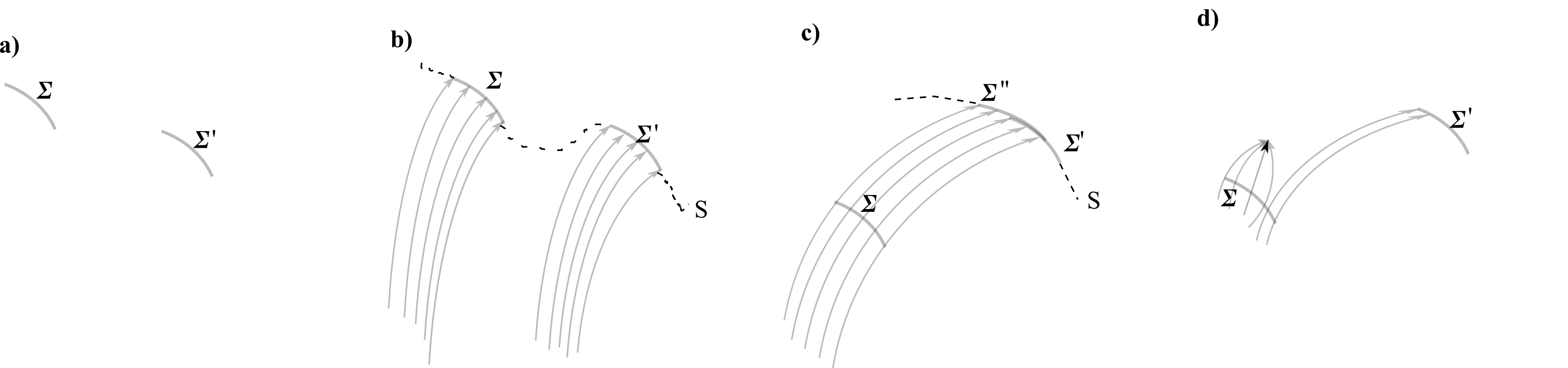
Figure 4: a) Consider now two hypersurface elements $\Sigma$ and $\Sigma^{\prime}$. b) Sometimes there will exist a section S orthogonal to the classical flow that includes both $\Sigma$ and $\Sigma^{\prime}$. Then via (30) or (33), P${}_{\Sigma\,\,\,\mbox{\scriptsize O}\mbox{\scriptsize R}\,\,\,\Sigma^{\prime}}$ = P${}_{\Sigma\,\bigcup\,\Sigma^{\prime}}$ just as for the Naïve Schrödinger Interpretation. c) However, if $\Sigma$ and $\Sigma^{\prime}$ do not lie on the same section, it is not directly like in the Naïve Schrödinger Interpretation. Now one can consider the flow-evolution of region $\Sigma$, say, so that it lies in a section that extends $\Sigma^{\prime}$; one can now compose $\Sigma^{\prime}$ and $\Sigma^{\prime\prime}$ just like one composed in case a). d) Moreover there need not always exist a section that extends $\Sigma^{\prime}$ whilst also containing a flow evolution image $\Sigma^{\prime\prime}$ of $\Sigma$. The construction of counterexamples, however, can avoid this case. What this case represents is that the composition of Halliwell’s implementation is not always reducible to a parallel of the Naïve Schrödinger Interpretation’s composition. Sometimes local sections and meshing conditions between them suffice for composition, but this does not always hold either. These non-existences reflect that some flows can be pathological/exhibit breakdowns in well-definedness or smoothness.

One way out of Caveat 3) is that QM may require modifying such as to obey an intuitionistic logic [115, 116], which is distributive. I also note that regions are conceptually different in this kind of approach (they are now primary themselves rather than ‘made up of’ some notion of points that are held to be primary), so that this possibility lies outside the scope of the present paper. It is also worth mentioning that [in e.g. [54, 58, 14]] proposition–projector association makes better sense than evoking regions, at the quantum level. This covers e.g. the case of the Isham–Linden approach to Histories Theory ([59, 58, 60] see also [117]), the Conditional Probabilities Interpretation [c.f. (10)], or Records within Histories theory [56, 62]. The main atemporal part of Isham and Doering [116] could also be viewed an underlying structure for Records Theory.

8.3 Halliwell 2009 type extension

Extending Halliwell’s 2009 work to the RPM arena mostly concerns defining class operators somewhat differently so as to get these to be better-behaved as regards the quantum Zeno effect. In detail, [64] amonnts to using an impenetrable barrier potential whilst [67, 68] corresponds to a slightly penetrable barrier potential. This amounts to the region in question being taken to contain a potential, with the class operator being the corresponding S-matrix and the slightly penetrable case representing a softening in the usual sense of scattering theory (albeit in configuration space rather than in space). [The smoothed-out case manages to avoid the quantum Zeno effect in addition to managing to still be compatible with the (quadratic, not for now linear) constraint.] Similar mathematics arises in the arrival time problem of QM [66, 112].

8.4 Quadrilateralland extension

Scaled $N$-stop metrolands RPM’s straightforwardly lie already within the Halliwell 2003 scheme. The quadrilateralland counterpart of the present paper is rather more complicated and may be worked out once quantization, the Semiclassical Approach and Histories Theory have been considered for that model.

8.5 More minimalist alternatives

The Gambini–Porto–Pullin approach [118] is a competitor insofar as it is a timeless/semiclassical combination (their work with Torterolo [119] furthermore combines this with ideas about observables). Thus it is similarly motivated to Halliwell’s approach and similarly applicable to Problem of Time and other issues in the foundations of Quantum Cosmology. It can also be investigated in the RPM arena. Arce [120] has provided a distinct combined Conditional Probabilities Interpretation–semiclassical scheme.

8.6 Conceptual analogy between RPM shapes and LQG knots

There is a loose conceptual analogy between pure-shape RPM’s shapes or scaled RPM’s scale-and-shapes (classical resolutions of the linear constraints) and LQG’s knot states [121] (quantum resolutions of the linear constraints). Loops themselves are analogous to preshapes [i.e. the configurations prior to the main part of the reduction – Dil($d$) but not Rot($d$) taken out for RPM’s or $SU(2)$ but not Diff($\Sigma$) taken out for LQG]. Passing to knot equivalence classes of loops is then analogous to the transformations used in [24, 25, 14] unveil the shape space/relational space variables. However the transformations in Sec 2 and 3 of [14] for RPM’s are purely configuration space manoeuvres, whereas passing to Ashtekar variables is itself a canonical transformation. Thus RPM’s fit better the philosophy of the central importance of the configuration space [17, 38] (as opposed to phase space or of any ‘polarizations’ of it that aren’t physically configurations). More ambitiously, might one be able to extend Halliwell’s class operator construction to LQG, so as to be able to, at least formally, write down a (perhaps partial) set of complete observables as a subset of the linear constraint complying knots? [I.e. a tentative search for a fully-fledged Unicorn.] This goes beyond the currently-known geometrodynamical minisuperspace scope of Halliwell’s class operators, but is an interesting direction in which to try to extend this scope; this discussion is further motivated by how Schroeren [122] has recently considered Hartle-type class functions for LQG, and is currently investigating Halliwell-type counterparts.

Acknowledgements I thank Mr Eduardo Serna, Professor Marc Lachi$\grave{\mbox{e}}$ze-Rey and especially Professor Jonathan Halliwell for discussions (and Jonathan also for pointing out various references and complications). This work was funded by a grant from the Foundational Questions Institute (FQXi) Fund, a donor-advised fund of the Silicon Valley Community Foundation on the basis of proposal FQXi-RFP3-1101 to the FQXi. I thank also Theiss Research and the CNRS for administering this grant. I thank also Professors Marc Lachi$\grave{\mbox{e}}$ze-Rey and David Langlois for APC travel money used for part of this project. I furtherly thank Professor Marc Lachi$\grave{\mbox{e}}$ze-Rey for help with my career. I thank my wife Claire, Amelia, Sophie and Sophie for support, and my friends Anya, Bryony, Hannah, Hettie, Amy, Duke, Zander, Sharon, Lynnette and Becky too.

Appendix A Various attitudes to environments in Quantum Cosmological models

For the RPM’s considered, scale dominates shape so as to model the small inhomogeneous fluctuations of the cosmological arena. There is then a fork as to whether to model this with a notion of environment.

Attitude 1) On the one hand, the 3-particle RPM has hitherto been taken as a whole-universe model. This most ideal interpretation is a lot less robust to assuming existence of additional particles whose contributions are then to be traced over (as compared with minisuperspace modelling having little problem with inclusion of an environment since one assumes there that this model sits in some kind of neglected environment of small inhomogeneous fluctuations). The issue then is justifying the latter parts of [64, 63] (or, even more so, the elsewise more correct [67, 68]) in the absense of an environment; this costs us e.g. lines (95-99) in the triangleland example. I note however that in the Halliwell 2009 parallel, configuration space regions that are large enough need no environment. As such, our next port of call (Paper II) is the RPM counterpart of Halliwell 2009 rather than further discussions of environment or its lack in the Halliwell 2003 context.

Attitude 2) Alternatively, study scale alone and use shape as an environment. This suffers from over-simpleness of the original system, but this is alleviated once one considers the shape perturbations about this.

Attitude 3) Study a small set of particles (say a triangle of particles) that are taken to dominate over the cloud of other particles, which make small and averaged-out contributions. These other particles are taken to be negligible in terms of most of their physical effects, but are still permitted to serve as an environment for decoherence and accompanying approximate information storage. Even 1 particle’s worth of environment can serve as a nontrivial environment [62]. This offers a second resolution to ‘losing [63]’s environment’: arguing that it was hitherto negligible in the study but is nevertheless available at this stage of the study as an environment.

References

- [1]
- [2] B.S. DeWitt, Phys. Rev. 160 1113 (1967).
- [3] J.A. Wheeler, in Battelle Rencontres: 1967 Lectures in Mathematics and Physics ed. C. DeWitt and J.A. Wheeler (Benjamin, N.Y. 1968).
- [4] K.V. Kuchař, in Quantum Gravity 2: a Second Oxford Symposium ed. C.J. Isham, R. Penrose and D.W. Sciama (Clarendon, Oxford 1981).
- [5] K.V. Kuchař, in Conceptual Problems of Quantum Gravity, eds. A. Ashtekar and J. Stachel (Birkhäuser, Boston, 1991).
- [6] K.V. Kuchař, in Proceedings of the 4th Canadian Conference on General Relativity and Relativistic Astrophysics, ed. G. Kunstatter, D. Vincent and J. Williams (World Scientific, Singapore, 1992).
- [7] C.J. Isham, in Integrable Systems, Quantum Groups and Quantum Field Theories ed. L.A. Ibort and M.A. Rodríguez (Kluwer, Dordrecht 1993), gr-qc/9210011.
- [8] K.V. Kuchař 1993, in General Relativity and Gravitation 1992, ed. R.J. Gleiser, C.N. Kozameh and O.M. Moreschi (Institute of Physics Publishing, Bristol 1993), gr-qc/9304012.
- [9] K.V. Kuchař, in The Arguments of Time, ed. J. Butterfield (Oxford University Press, Oxford 1999).
- [10] C. Rovelli, Quantum Gravity (Cambridge University Press, Cambridge 2004).
- [11] C. Kiefer, Quantum Gravity (Clarendon, Oxford 2004).
- [12] L. Smolin, Problem of Time Course (2008), available in video form at http://pirsa.org/C08003.
- [13] E. Anderson, in Classical and Quantum Gravity: Theory, Analysis and Applications ed. V.R. Frignanni (Nova, New York 2012), arXiv:1009.2157.
- [14] E. Anderson, arXiv:1111.1472.
- [15] E. Anderson, “The Problem of Time”, invited review for Annalen der Physik, arXiv:1206.2403.
- [16] J.B. Barbour and B. Bertotti, Proc. Roy. Soc. Lond. A382 295 (1982).
- [17] J.B. Barbour, Class. Quantum Grav. 11 2853 (1994).
- [18] J.B. Barbour, Class. Quantum Grav. 11 2875 (1994); The End of Time (Oxford University Press, Oxford 1999).
- [19] J.B. Barbour, Class. Quantum Grav. 20 1543 (2003), gr-qc/0211021.
- [20] E. Anderson, Class. Quantum Grav. 23 2469 (2006), gr-qc/0511068.
- [21] E. Anderson, Class. Quantum Grav. 23 2491 (2006), gr-qc/0511069.
- [22] E. Anderson, Class. Quantum Grav. 24 2935 (2007), gr-qc/0611007.
- [23] E. Anderson, Class. Quantum Grav. 24 5317 (2007), gr-qc/0702083.
- [24] E. Anderson, Class. Quantum Grav. 25 025003 (2008), arXiv:0706.3934.
- [25] E. Anderson, arXiv:1001.1112.
- [26] E. Anderson Proceedings of the Rio de Janeiro Marcel Grossmann Meeting 2003, arXiv:gr-qc/0312037; AIP Conf. Proc. 861 285 (2006), gr-qc/0509054; Proceedings of Paris 2009 Marcel Grossman Meeting (World Scientific, Singapore 2012), arXiv:0908.1983; J.B. Barbour, arXiv:1105.0183; E. Anderson and S.A.R. Kneller, “Relational Quadrilateralland. II. The Quantum Theory”, forthcoming; E. Anderson, “Relational Quadrilateralland. III. As a Problem of Time Arena”, forthcoming.
- [27] E. Anderson, Int. J. Mod. Phys. D18 635 (2009), arXiv:0709.1892; in Proceedings of the Second Conference on Time and Matter, ed. M. O’Loughlin, S. Stanič and D. Veberič (University of Nova Gorica Press, Nova Gorica, Slovenia 2008), arXiv:0711.3174.
- [28] E. Anderson, Class. Quantum Grav. 26 135020 (2009), arXiv:0809.1168.
- [29] E. Anderson, Class. Quantum Grav. 26 135021 (2009), arXiv:0809.3523.
- [30] E. Anderson and A. Franzen, Class. Quantum Grav. 27 045009 (2010), arXiv:0909.2436.
- [31] E. Anderson, Gen. Rel. Grav. 43 1529 (2011), arXiv:0909.2439.
- [32] E. Anderson, Class. Quantum Grav. 28 065011 (2011), arXiv:1003.4034.
- [33] E. Anderson, arXiv:1005.2507.
- [34] E. Anderson, Class. Quant. Grav. 28 185008 (2011), arXiv:1101.4916.
- [35] E. Anderson, arXiv:1009.2161; arXiv:1102.2862; N.H. Kuiper, Math. Ann. 208 175 (1974); G.W. Gibbons and C.N. Pope, Commun. Math. Phys. 61 239 (1978); A.J. MacFarlane, J. Phys. A: Math. Gen. 36 7049 (2003).
- [36] E. Anderson, arXiv:1202.4186.
- [37] E. Anderson, arXiv:1202.4187.
- [38] E. Anderson, arXiv:1205.1256.
- [39] E. Anderson, “Machian Time Is To Be Abstracted From What Change?”, forthcoming.
- [40] E. Anderson, “Machian Classical and Semiclassical Emergent Times”, forthcoming.
- [41] E. Anderson, Class. Quantum Grav. 27 045002 (2010), arXiv:0905.3357.
- [42] B.S. DeWitt, Rev. Mod. Phys. 29 377 (1957).
- [43] C.W. Misner, in Magic Without Magic: John Archibald Wheeler ed. J. Klauder (Freeman, San Fransisco 1972).
- [44] T. Christodoulakis and J. Zanelli, Nuovo Cim. B93 1 (1986); J.J. Halliwell, Phys. Rev. D38 2468 (1988); I. Moss, Ann. Inst. H. Poincaré 49 341 (1988); M.P. Ryan and A.V. Turbiner, Phys. Lett. A333 30 (2004), quant-ph/0406167.
- [45] S.W. Hawking and D.N. Page, Nucl. Phys. B264 185 (1986).
- [46] P.A.M. Dirac, Lectures on Quantum Mechanics (Yeshiva University, New York 1964).
- [47] C.J. Isham, in Relativity, Groups and Topology II ed. B. DeWitt and R. Stora (North-Holland, Amsterdam 1984).
- [48] S.A. Hojman, K.V. Kuchař and C. Teitelboim, Ann. Phys. N.Y. 96 88 (1976).
- [49] See e.g R.D. Sorkin, gr-qc/0309009; See, e.g, A. Perez, Class. Quantum Grav. 20 R43 (2003), gr-qc/0301113; R.M. Williams and P.A. Tuckey, Class. Quant. Grav. 9 1409 (1992); M. Bojowald, Class. Quant. Grav. 18 L109 (2001), arXiv:gr-qc/0105113 J. Ambjorn, A. Gorlich, J. Jurkiewicz, R. Loll, J. Gizbert-Studnicki and T. Trzesniewski, Nucl. Phys. B849 144 (2011) arXiv:1102.3929. F. Conrady and L. Freidel, Phys. Rev. D78 104023 (2008), arXiv:0809.2280; J. Hackett and S. Speziale, Class. Quant. Grav. 24 1525 (2007), arXiv:gr-qc/0611097.
- [50] J.S. Bell, in The Physicists’ Concept of Nature (Dirac Festschrift) ed. Mehra (Reidel, Dordrecht 1973); p.52 in Speakable and Unspeakable in Quantum Mechanics (Cambridge University Press, Cambridge 1987).
- [51] J.S. Bell, in Quantum Gravity 2. A Second Oxford Symposium eds. C.J. Isham, R. Penrose and D.W. Sciama (Clarendon, Oxford, 1981).
- [52] J.J. Halliwell and S.W. Hawking, Phys. Rev. D31, 1777 (1985).
- [53] W. Unruh and R.M. Wald, Phys. Rev. D40 2598 (1989).
- [54] D.N. Page and W.K. Wootters, Phys. Rev. D27, 2885 (1983).
- [55] D.N. Page, Int. J. Mod. Phys. D5 583 (1996), quant-ph/9507024; in Consciousness: New Philosophical Essays ed. Q. Smith and A. Jokic (Oxford University Press, Oxford 2002), quant-ph/0108039.
- [56] M. Gell-Mann and J.B. Hartle, Phys. Rev. D47 3345 (1993).
- [57] J.B. Hartle, in Gravitation and Quantizations: Proceedings of the 1992 Les Houches Summer School ed. B. Julia and J. Zinn-Justin (North Holland, Amsterdam 1995), gr-qc/9304006; Phys. Scripta T76 67 (1998), gr-qc/9712001.
- [58] C.J. Isham and N. Linden, J. Math. Phys. 36 5392 (1995), gr-qc/9503063.
- [59] C.J. Isham and N. Linden, J. Math. Phys. 35 5452 (1994), gr-qc/9405029.
- [60] C.J. Isham and N. Linden, J. Math. Phys. 35 5452 (1994), gr-qc/gr-qc/9405029; C.J. Isham, N. Linden, N. Savvidou and S. Schreckenberg, J. Math. Phys. 39 1818 (1998), quant-ph/9711031. C. Anastopoulos, J. Math. Phys. 41 617 (2000), gr-qc/9903026; K.N. Savvidou, Class. Quant. Grav. 18 3611 (2001), gr-qc/0104081; J. Math. Phys. 43 3053 (2002), gr-qc/0104053; Class. Quant. Grav. 21 615 (2004), gr-qc/0306034; 631 (2004), gr-qc/0306036; C. Anastopoulos and N. Savvidou, Class. Quantum Grav. 22 1841 2005, gr-qc/0410131; S. Kessari, Class. Quant. Grav. 24 1303 (2007), arXiv:gr-qc/0605105.
- [61] M. Gell-Mann and J.B. Hartle, arXiv:1106.0767.
- [62] J.J. Halliwell, Phys. Rev. D60 105031 (1999), quant-ph/9902008.
- [63] J.J. Halliwell and J. Thorwart, Phys. Rev. D65 104009 (2002), gr-qc/0201070.
- [64] J.J. Halliwell, in The Future of Theoretical Physics and Cosmology (Stephen Hawking 60th Birthday Festschrift volume) ed. G.W. Gibbons, E.P.S. Shellard and S.J. Rankin (Cambridge University Press, Cambridge 2003), arXiv:gr-qc/0208018.
- [65] J.J. Halliwell and J. Thorwart, Phys. Rev. D64 124018 (2001), gr-qc/0201070; J.J. Halliwell and P.J. Dodd, Phys. Rev. D67 105018 (2003), quant-ph/0301104; J.J. Halliwell and P. Wallden, Phys. Rev. D73 024011 (2006), gr-qc/0509013.
- [66] J.J Halliwell and J.M. Yearsley, Phys. Rev. A79 062101 (2009), arXiv:0903.1957; Phys. Lett. A 374 154 (2009), arXiv:0903.1958; J. Phys. A-Math. Theor. 43 445303 (2010) arXiv:1006.4788; J.M. Yearsley, for Proceedings of DICE 2010 Conference, arXiv:1012.2575.
- [67] J.J. Halliwell, Phys. Rev. D80 124032 (2009), arXiv:0909.2597.
- [68] J.J. Halliwell, J. Phys. Conf. Ser. 306 012023 (2011), arXiv:1108.5991.
- [69] J.B. Barbour, B.Z. Foster and N. Ó Murchadha, Class. Quantum Grav. 19 3217 (2002), gr-qc/0012089; E. Anderson and J.B. Barbour, Class. Quantum Grav. 19 3249 (2002), gr-qc/0201092; N. Ó Murchadha, Int. J. Mod. Phys A20 2717 (2002); E. Anderson, Gen. Rel. Grav. 36 255 (2004), gr-qc/0205118; Phys. Rev. D68 104001 (2003), gr-qc/0302035; N. Ó Murchadha, gr-qc/0305038; E. Anderson, “Geometrodynamics: Spacetime or Space?” (Ph.D. Thesis, University of London 2004), gr-qc/0409123; in Classical and Quantum Gravity Research, ed. M.N. Christiansen and T.K. Rasmussen (Nova, New York 2008), arXiv:0711.0285; E. Anderson, J.B. Barbour, B.Z. Foster, B. Kelleher and N. Ó Murchadha, Class. Quantum Grav 22 1795 (2005), gr-qc/0407104; gr-qc/0404099.
- [70] E. Anderson, in General Relativity Research Trends, Horizons in World Physics 249 ed. A. Reimer (Nova, New York 2005), gr-qc/0405022; Stud. Hist. Phil. Mod. Phys. 38 15 (2007), gr-qc/0511070.
- [71] E. Anderson, Class. Quantum Grav. 25 175011 (2008), arXiv:0711.0288.
- [72] T. Thiemann, Modern Canonical Quantum General Relativity (Cambridge University Press, Cambridge 2007).
- [73] See D.S. Berman and M.J. Perry, JHEP 1106:074 (2011) arXiv:1008.1763 and references therein.
- [74] C.J. Isham & K.V. Kuchař, Ann. Phys. (NY) 164 288; 316 (1985).
- [75] S. Carlip, Quantum Gravity in 2 + 1 Dimensions (Cambridge University Press, Cambridge 1998).
- [76] I. Kouletsis and K.V. Kuchař , Phys. Rev. D65 125026 (2002), arXiv:gr-qc/0108022.
- [77] P.A.M. Dirac, Rev. Mod. Phys. 21 392 (1949).
- [78] C. Rovelli and L. Smolin, Nu. Phys. B331 80 (1990).
- [79] P. Hájíček, J. Math. Phys. 36 4612 (1996), gr-qc/9412047; C.J. Isham and P. Hájíček, J. Math. Phys. 37 3522 (1996), gr-qc/9510034; J. Pullin and R. Gambini, in 100 Years of Relativity. Space-Time Structure: Einstein and Beyond ed. A. Ashtekar (World Scientific, Singapore 2005).
- [80] P. Hájíček, gr-qc/9903089; P. Hájíček and J. Kijowski, Phys. Rev. D61 024037 (2000), gr-qc/99080451; G. Belot and J. Earman, in Physics Meets Philosophy at the Planck Scale, ed. C. Callender and N. Huggett, Cambridge University Press (2000). J. Earman, Phil. Sci. 69 S209 (2002); H. Farajollahi, gr-qc/0406024; C. Wüthrich, “Approaching the Planck Scale from a Generally Relativistic Point of View: A Philosophical Appraisal of Loop Quantum Gravity” (Ph.D Thesis, Pittsburgh 2006); J.B. Barbour and B.Z. Foster, arXiv:0808.1223.
- [81] K.V. Kuchař , J. Math. Phys. 22 2640 (1981).
- [82] C.G. Torre, Phys. Rev. D48 2373 (1993), gr-qc/9306030.
- [83] C.G. Torre, Phys. Rev. Lett 70 3525 (1993); C.G. Torre and I.M. Anderson, Commun. Math. Phys. 176 479 (1996), gr-qc/9404030; S. Carlip, Rept. Prog. Phys. 64 885 (2001), gr-qc/0108040.
- [84] E. Anderson, version 3 of arXiv:1111.1472, forthcoming shortly.
- [85] C. Rovelli, p. 126 in Conceptual Problems of Quantum Gravity ed. A. Ashtekar and J. Stachel (Birkhäuser, Boston, 1991); Phys. Rev. D43 442 (1991); D44 1339 (1991).
- [86] S. Carlip, Phys. Rev. D42 2647 (1990); Class. Quantum Grav. 8 5 (1991).
- [87] C. Rovelli, Phys. Rev. D65 044017 (2002), arXiv:gr-qc/0110003; 65 124013, gr-qc/0110035.
- [88] B. Dittrich, Class. Quant. Grav. 23 6155 (2006), gr-qc/0507106.
- [89] G. Mackey, Mathematical Foundations of Quantum Mechanics (Benjamin, New York 1963).
- [90] See e.g. R. Omns, J. Stat. Phys. 357 57 (1989); C. Anastopoulos, Phys. Rev. E53 4711 (1996), quant-ph/9506031; J.J. Halliwell, arXiv:1207.0992.
- [91] J.J. Halliwell, Phys. Rev. D36 3626 (1987).
- [92] E.P. Wigner Phys. Rev. 40 749 (1932).
- [93] M. Hillery, R.F. O’Connell, M.O. Scully and E.P. Wigner, Phys. Rep. 106 121 (1984); P. Carruthers and F. Zacariasen, Rev. Mod. Phys. 55 245 (1984); V.I. Tatarskii, Sov. Phys. Usp. 26 311 (1983); N. Balsz and B.K. Jennings, Phys. Rep. 104 347 (1984); M. Brack and R. Bhaduri, Semiclassical Physics (Addison-Wesley, Reading, Massachusetts 1997).
- [94] I. Bialynicki-Birula, M. Cieplak and J. Kaminski, Theory of Quanta (Oxford University Press, New York 1992).
- [95] J.J. Halliwell, in Proceedings of the 13th International Conference on General Relativity and Gravitation ed. R.J. Gleiser, C.N. Kozameh and O.M. Moreschi (IOP, Bristol 1992), gr-qc/9208001.
- [96] N. Mott, Proc. Roy. Soc. Lon. A126 79 (1929).
- [97] See e.g. R.P. Feynman and A.R. Hibbs, Quantum Mechanics and Path Integrals (McGraw-Hill, New York 1965).
- [98] D.G. Kendall, D. Barden, T.K. Carne and H. Le, Shape and Shape Theory (Wiley, Chichester 1999).
- [99] R.G. Littlejohn and M. Reinsch, Rev. Mod. Phys. 69 213 (1997).
- [100] See e.g. C. Marchal, Celestial Mechanics (Elsevier, Tokyo 1990).
- [101] V. Aquilanti, S. Cavalli and G. Grossi, J. Chem. Phys. 85 1362 (1986).
- [102] A.J. Dragt, J. Math. Phys. 6 533 (1965).
- [103] R.M. Wald, General Relativity (University of Chicago Press, Chicago 1984).
- [104] J. Winter, Phys. Rev. D32 1871 (1985); H.E. Kandrup, Phys. Rev D37 2165 (1988); E. Calzetta, S. Habib and B.L. Hu, Phys. Rev D40 381 (1989); S. Habib and H.E. Kandrup, Ann. Phys. 191 335 (1989).
- [105] O.A. Fonarev, Sov. Phys. JETP 33 759 (1990).
- [106] Z-J. Liu and M. Qian, Trans AMS 331 321 (1992).
- [107] J. Underhill, J. Math. Phys. 19 1932 (1978).
- [108] N.P. Landsmann, J. Geom. Phys. 12 93 (1993).
- [109] K.V. Kuchař, J. Math. Phys. 13 758 (1972).
- [110] K.V. Kuchar, Phys. Rev. D50 3961 (1994), arXiv:gr-qc/9403003.
- [111] C.G. Torre, Class. Quant. Grav. 23 1543 (2006) arXiv:gr-qc/0508008.
- [112] J.J.Halliwell, arXiv:0801.4308; J.M. Yearsley, Phys. Rev. A82 012116 (2010), arXiv:1003.6079; J.J. Halliwell and J.M.Yearsley, arXiv:1205.3773; J.M. Yearsley, D.A. Downs, J.J. Halliwell and A.K. Hashagen, Phys. Rev. A84 022109 (2011), arXiv:1106.4767.
- [113] M. Bojowald, P.A. Hoehn and A. Tsobanjan, Class. Quant. Grav. 28 035006 (2011), arXiv:1009.5953; Phys. Rev. D83 125023 (2011), arXiv:1011.3040; P.A. Hoehn, E. Kubalova and A. Tsobanjan, arXiv:1111.5193; P.A Hoehn, arXiv:1110.5631.
- [114] C.J. Isham, J. Math. Phys. 35 2157 (1994), gr-qc/9308006; writeup of lecture given at Conference “Theories of Fundamental Interactions”, Maynooth Eire 24–26 May 1995, quant-ph/9506028.
- [115] C.J. Isham and J. Butterfield, Found. Phys. 30 1707 (2000), arXiv:gr-qc/9910005.
- [116] A. Doering and C.J. Isham, J. Math. Phys. 49 053515 (2008), quant-ph/0703060; 053516, quant-ph/0703062; 053517, quant-ph/0703064; 053518, quant-ph/0703066; A. Doering and C. Isham, to appear in “New Structures in Physics” ed R. Coecke, arXiv:0803.0417; A. Doering, for Proceedings of workshop “Recent Developments in Quantum Field Theory”, MPI MIS Leipzig, July 2007”, arXiv:0712.4003; C.J. Isham, in “Deep Beauty” ed. H. Halvorson (Cambridge University Press, Cambridge 2010), arXiv:1004.3564; see also C. Flori, “Approaches To Quantum Gravity” (Ph.D. Thesis, Humboldt University, Berlin 2009), arXiv:0911.2135; arXiv:1106.5660.
- [117] C. Flori, J. Math. Phys. 51 (2010) 053527, arXiv:0812.1290.
- [118] R. Gambini and R.A. Porto, Phys. Rev. D63 105014 (2001), arXiv:gr-qc/0101057; R. Gambini, R. Porto and J. Pullin, New J. Phys. 6 45 (2004), arXiv:gr-qc/0402118; Phys. Rev. D70 124001 (2004), arXiv:gr-qc/0408050; Gen. Rel. Grav. 39 1143 (2007), gr-qc/0603090.
- [119] R. Gambini, R. Porto, S. Torterolo and J. Pullin, Phys. Rev. D79 041501 (2009), arXiv:0809.4235.
- [120] J.C. Arce, arXiv:1202.4638.
- [121] R. Gambini and J. Pullin Loops, Knots, Gauge Theories and Quantum Gravity (Cambridge University Press, Cambridge 1996).
- [122] D. Schroeren, arXiv:1206.4553.