Emergence of grouping in multi-resource minority game dynamics

Abstract

The Minority Game (MG) has become a paradigm to probe complex social and economical phenomena where adaptive agents compete for a limited resource, and it finds applications in statistical and nonlinear physics as well. In the traditional MG model, agents are assumed to have access to global information about the past history of the underlying system, and they react by choosing one of the two available options associated with a single resource. Complex systems arising in a modern society, however, can possess many resources so that the number of available strategies/resources can be multiple. We propose a class of models to investigate MG dynamics with multiple strategies. In particular, in such a system, at any time an agent can either choose a minority strategy (say with probability $p$) based on available local information or simply choose a strategy randomly (with probability $1-p$). The parameter $p$ thus defines the minority-preference probability, which is key to the dynamics of the underlying system. A striking finding is the emergence of strategy-grouping states where a particular number of agents choose a particular subset of strategies. We develop an analytic theory based on the mean-field framework to understand the “bifurcation” to the grouping states and their evolution. The grouping phenomenon has also been revealed in a real-world example of the subsystem of $27$ stocks in the Shanghai Stock Market’s Steel Plate. Our work demonstrates that complex systems following the MG rules can spontaneously self-organize themselves into certain divided states, and our model represents a basic mathematical framework to address this kind of phenomena in social, economical, and even political systems.

I Introduction

The Minority Game (MG) was originated from the El Farol bar problem in game theory first conceived by Arthur in 1994 Arthur:1994 , where a finite population of people try to decide, at the same time, whether to go to the bar on a particular night. Since the capacity of the bar is limited, it can only accommodate a small fraction of all who are interested. If many people choose to go to the bar, it will be crowded, depriving the people of the fun and thereby defying the purpose of going to the bar. In this case, those who choose to stay home are the winners. However, if many people decide to stay at home then the bar will be empty, so those who choose to go to the bar will have fun and they are the winners. Apparently, no matter what method each person uses to make a decision, the option taken by majority of people is guaranteed to fail and the winners are those that choose the minority one. Indeed, it can be proved that, for the El Farol bar problem there are mixed strategies and a Nash-equilibrium solution does exist, in which the option taken by minority wins Gintis:2009 . A variant of the problem was subsequently proposed by Challet and Zhang, named as an MG problem CZ:1997 , where a player among an odd number of players chooses one of the two options at each time step. Subsequently, the model was studied in a series of works CM:1999 ; CMZ:2000 ; MMM:2004 ; BMM:2007 ; RMR:1999 ; PBC:2000 ; ZWZYL:2005 ; EZ:2000 ; KSB:2000 ; Slanina:2000 ; ATBK:2004 ; JHH:1999 ; HJJH:2001 ; LCHJ:2004 ; TCHJ:2005 ; CMM:2008 ; BMFM:2008 ; XWHZ:2005 ; ZZZH:2005 . In physics, MG has received a great deal of attention from the statistical-mechanics community, especially in terms of problems associated with non-equilibrium phase transitions Moro:2004 ; CMZ:2005 ; YZ:2008 .

In the current literature, the setting of MG is that there is a single resource with players’ two possible options (e.g., in the El Farol bar problem there is a single bar and the options of agents are either going to the bar or not), and an agent is assumed to react to available global information about the history of the system by taking on an alternative option that is different than the current one it is taking. The outstanding question remains of the nonlinear dynamics of MG with multiple resources. The purpose of this paper is to present a class of multi-resource MG models. In particular, we assume a complex system with multiple resources and, at any time, an individual agent has $k>1$ resources/strategies to choose from. We introduce a parameter $p$, which is the probability that each agent responds based on its available local information by selecting a less crowded resource in an attempt to gain higher payoff. We call $p$ the minority-preference probability. We find, strikingly, as $p$ is increased, the phenomenon of grouping emerges, where the resources can be distinctly divided into two groups according to the number of their attendees. In addition, the number of stable pairs of groups also increases. We shall show that the grouping phenomenon plays a fundamental role in shaping the fluctuations of the system. The phenomenon will be demonstrated numerically and explained by a comprehensive analytic theory. An application to the analysis of empirical data from a real financial market will also be illustrated, where grouping of stocks (resources) appears. Our model is not only directly relevant to nonlinear and complex dynamical systems, but also applicable to social and economical systems.

Our multi-resource MG model is presented in Sec. II. The emergence of grouping phenomenon is demonstrated in Sec. III. A general theory is developed in Sec. IV to elucidate the dynamics of the emergence and evolution of the strategy groups. Concluding remarks are presented in Sec. VI.

II Multi-resource minority game model

We consider a complex, evolutionary-game type of dynamical system of $N$ interacting agents competing for multiple resources. Each agent will chose one resource in each round of the game. And, each resource has a limited capacity, i.e., the number of agents it can accommodate has an upper bound $n_{c}$. There are thus multiple strategies ($s=1$, $2$, $\cdots$, $k$, where $k$ is the maximum number of resources/strategies) available to each agent. On average, each strategy can accommodate $N/k$ agents, and we consider the simple case of $n_{c}=N/k$. Let $n_{s}$ be the number of agents selecting a particular strategy $s$. If $n_{s}\leq n_{c}$, the corresponding agents win the game and, consequently, $s$ is the minority strategy. However, if $n_{s}>n_{c}$, the associated resource is too crowded so that the strategy fails and the agents taking it lose the game, which defines the “majority strategy.” The optimal solution to the game dynamics is thus $n_{s}=n_{c}$.

In a real-world system, it is often difficult or even impossible for each agent to gain global information about the dynamical state of the whole system. It is therefore useful to introduce the concept of local information network in our multiple-resource MG model. At each time step, with probability $p$, namely the minority-preference probability, each agent acts based on local information that it gains by selecting one of the $k$ available strategies. In contrast, with probability $1-p$, an agent acts without the guidance of any local information. For the minority-preference case, agent $i$ has $d$ neighbors in the networked system. The required information for $i$ to react consists of all its neighbors’ strategies and, among them, the winners of the game, i.e., those neighboring agents choosing the minority strategies at the last time step. Let $\Pi=\{s_{m}\}$ be the set of minority strategies for $i$’s winning neighbors, where a strategy may appear a number of times, if it has been chosen by different winning neighbors. With probability $p$, agent $i$ will chose one strategy randomly from $\Pi$. Thus, the probability $P_{s}$ for strategy $s$ to be selected is proportional to the times it appears in $\Pi$, i.e., $P_{s}=N_{s}/Card(\Pi)$, where $Card(\Pi)$ is the number of elements in $\Pi$ and $N_{s}$ the times strategy $s$ appears in $\Pi$. If $\Pi$ is empty, $i$ will randomly select one from the $k$ available strategies. While, for the case that an agent selects a strategy without the guidance of any local information with probability $1-p$, it will either choose a different strategy randomly from the $k$ available ones with mutation probability $m$ ZWZYL:2005 , or inherit its strategy from the last time step with probability $1-m$.

III Numerical results

As a concrete example to illustrate the strategy-grouping phenomenon, we set $k=5$. Figures 1(a-c) show time series of $n_{s}$, the number of agents selecting each strategy $s$, for $p=0$, 0.45, and 1.0, respectively. For Fig. 1(a) where $p=0$, an agent makes no informed decision in that it changes strategy randomly with probability $m$ but stays with the original strategy with probability $1-m$. In this case, $n_{s}$’s appear random. For the opposite extreme case of $p=1$ [Fig. 1(c)], each agent makes well informed decisions based on available local information about the strategies used by its neighbors. In this case, the time series are quasiperiodic (a detailed analysis will be provided in Sec. IV). For the intermediate case of $p=0.45$ [Fig. 1(b)], agents’ decisions are partially informed. In this case, an examination of the time series points to the occurrence of an interesting grouping behavior: the 5 strategies, in terms of their selection by the agents, are divided into two distinct groups $g_{1}$ and $g_{2}$ that contain $k_{g_{1}}=2$ and $k_{g_{2}}=3$ resources, respectively. The time series associated with the smaller group exhibit larger fluctuations about its equilibrium.

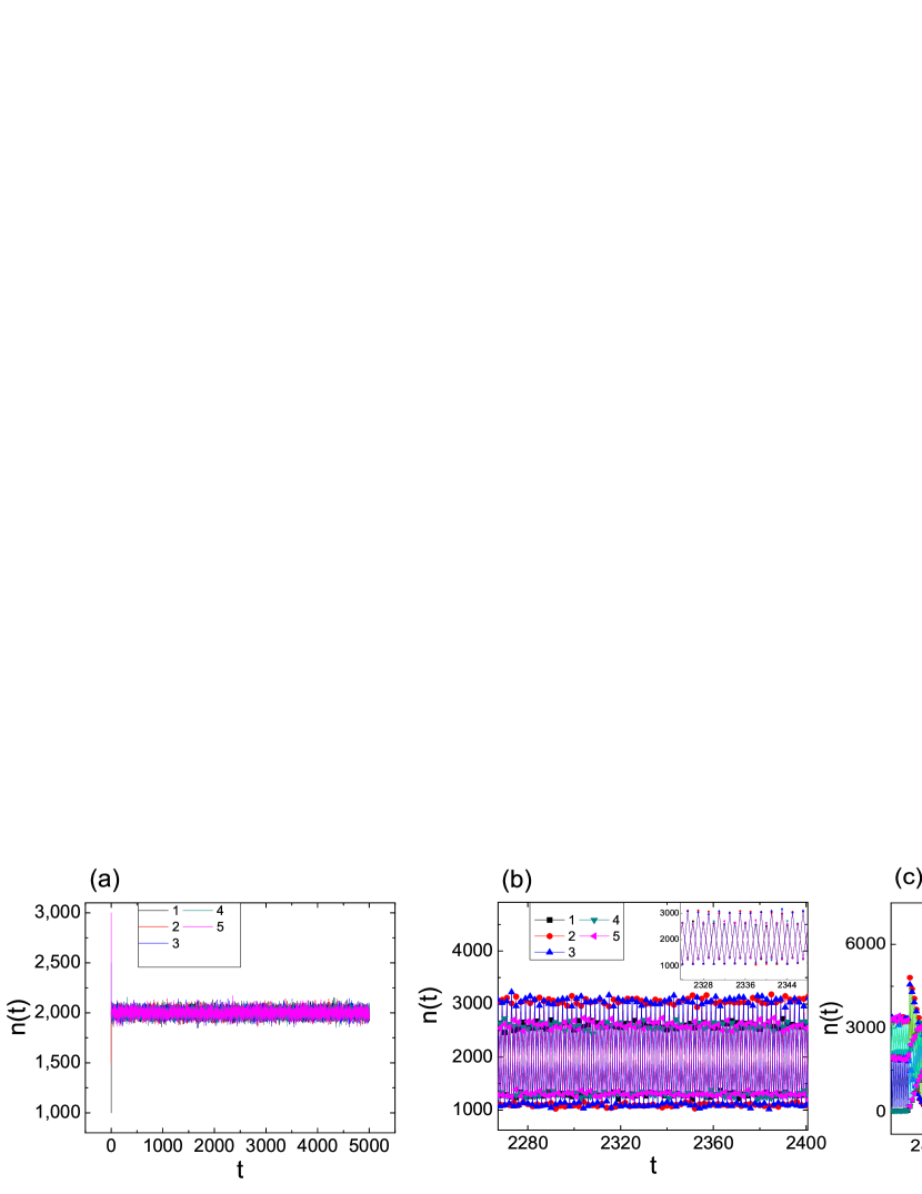
Figure 1: (Color online.) (a-b) For a square-lattice system of $N=10000$ agents, time series of the number of agents selecting each of the $k=5$ available strategies for $p=0$, 0.45, and 1.0, respectively. The probability of random alteration of strategy in the case of complete lack of local information is set to be $m=1$. A strategy grouping behavior can be seen in (b), where the whole strategy set is broken into two groups: one of two and another of three strategies.

To better characterize the fluctuating behaviors in the time series $n_{s}$, we calculate the variance $\sigma^{2}_{s}=\langle[n_{s}(t)-N/k]^{2}\rangle$ as a function of the system parameter $p$, where $\langle\cdot\rangle$ is the expectation values averaged over a long time interval, as shown in Fig. 2 on a logarithmic scale. We observe a generally increasing behavior in $\sigma^{2}_{s}$ with $p$ and, strikingly, a bifurcation-like phenomenon. In particular, for $p<p_{b}$, where $p_{b}$ is the bifurcation point, $\sigma^{2}$s for all strategies assume approximately the same value. However, for $p>p_{b}$, there are two distinct values for $\sigma^{2}$, signifying the aforementioned grouping behavior [Fig. 1(b)]. From Fig. 2, we also see that, after the bifurcation, the two branches of $\sigma^{2}$ are linear (on a logarithmic scale) and have approximately the same slope $a$, suggesting the following power-law relation: $\sigma^{2}_{g_{i}}={b_{g_{i}}p^{a}}$, for $i=1,2$, where $\log{(b_{g_{1}})}$ and $\log{(b_{g_{2}})}$ are the intercepts of the two lines in Fig. 2. We thus obtain

$$\frac{\sigma^{2}_{g_{1}}}{\sigma^{2}_{g_{2}}}=\frac{b_{g_{1}}}{b_{g_{2}}}.$$ (1)

In Sec. IV, we will develop a theory to explain the relations among the variances of the grouped strategies and to provide formulas for the amplitudes of the time series in Fig. 1 and the sizes of the groups (denoted by $k_{g_{1}}$ and $k_{g_{2}}$, respectively). Specifically, our theory predicts the following ratio between the variances of the two bifurcated branches:

$$\frac{\sigma^{2}_{g_{1}}}{\sigma^{2}_{g_{2}}}=(\frac{k_{g_{2}}}{k_{g_{1}}})^{2},$$ (2)

which is identical to the numerically observed ratio in Eq. (1), with the additional prediction that the strategies in the group of smaller size exhibit stronger fluctuations since the corresponding value of $\sigma^{2}$ is larger. Overall, the emergence of the grouping behavior in multiple-resource MGs, as exemplified in Fig. 2, resembles a period-doubling like bifurcation. While period-doubling bifurcations are extremely common in nonlinear dynamical systems, to our knowledge, in complex game systems a clear signature of such a bifurcation had not been reported previously.

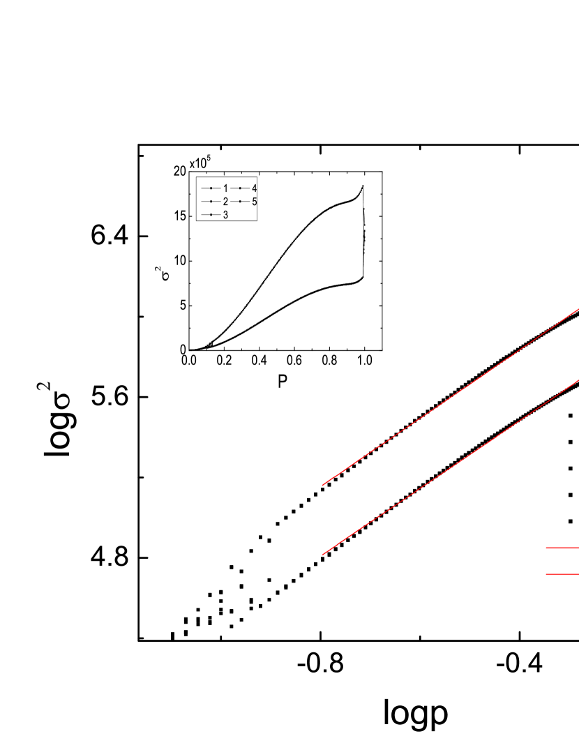
Figure 2: For the same system in Fig. 1, variance $\sigma^{2}$ of the time series $n_{s}$ as a function of $p$ on a logarithmic scale. A period-doubling like bifurcation occurs, at which a grouping behavior emerges. Inset is the same plot but on a linear scale.

A careful examination of the time-series for various $p$ has revealed that the strategy-grouping processes has already taken place prior to the bifurcation point $p_{b}$ in the variance $\sigma^{2}$, but all resulted grouping states are unstable. Take as an example the $5$-strategy system in Fig. 1. In principle, there can be two types of pairing groups: $(1,4)$ and $(2,3)$. For any grouping state, the following constraint applies:

$$k_{g_{1}}+k_{g_{2}}=k,\qquad k_{g_{1}}\cdot k_{g_{2}}\neq 0$$ (3)

There are in total $k/2$ (if $k$ is even) or $(k-1)/2$ (if $k$ is odd) possible grouping states for the system with $k$ available strategies. However, the grouping states are not stable for $p<p_{b}$. What happens is that a strategy can remain in one group but only for a finite amount of time before switching to a different group. Assume that the sizes of the original two pairing groups are $(k_{g_{1}}$ and $k_{g_{2}})$, respectively. The sizes of the new pair of groups are thus $(k_{g_{1}}\pm 1$ and $k_{g_{2}}\mp 1)$, as stipulated by Eq. (3). Associated with switching to a different pair of groups, the amplitudes of the time series $n_{s}$ for each strategy also change. As the bifurcation parameter $p$ is increased, the stabilities of different pairs of grouping states also change. At the bifurcation point $p_{b}$, one particular pair of groups becomes stable, such as the grouping state $(2,3)$ in Fig. 2.

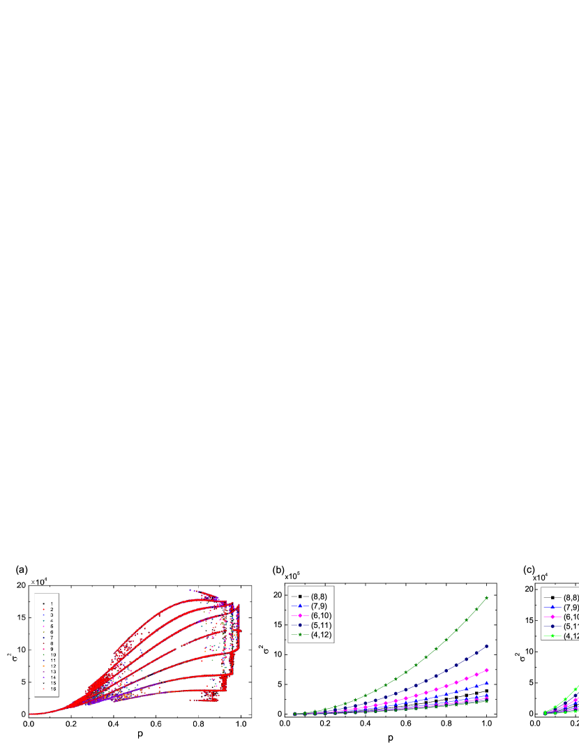
Figure 3: (Color online.) For a multiple-resource MG system of $N=10000$ agents on a square lattice and $k=16$ available strategies, (a) numerically obtained bifurcation-like behavior that leads to the emergence of various pairs of grouping states [e.g, (8,8), (4,12), etc.], (b) predicted bifurcation from mean-field theory (Sec. IV), and (c) results from an improved mean-field theory (Sec. IV). The probability of random selection in the absence of local information is set to be $m=1$.

The bifurcation-like phenomenon and the emergence of various strategy-grouping states are general for multiple-resource MG game dynamics. For example, Fig. 3 shows $\sigma^{2}$ as a function of $p$ for a system with $k=16$ available strategies. There are in total 8 possible grouping states, ranging from $(8,8)$ to $(1,15)$. As $p$ is increased, the grouping states $(8,8)$, $(7,9)$, $(6,10)$, $(5,11)$ and $(4,12)$ become stable one after another, as can be seen from the appearance of their corresponding branches in Fig. 3. The behavior can be understood theoretically through a stability analysis (Sec. IV).

Another phenomenon revealed by Fig. 3 is the merging of bifurcated branches. For example, as $p$ is increased through about 0.8, the grouping states disappear one after another in the reverse order as they initially appeared. This can also be understood through the stability analysis (Sec. IV).

IV Theory

Here we develop an analytic theory to understand the emergence, characteristics, and evolutions of the strategy groups.

IV.1 Relationship among variance, amplitude and group size

In general, for a multiple-resource MG system of $N$ agents, as the parameter $p$ is increased so that agents become more likely to make informed decision for strategy selection, the available strategies can be divided into pairs of groups. The example in Fig. 1(b) presents a case where there are two distinct strategy groups $g_{1}$ and $g_{2}$, which contain $k_{g_{1}}$ and $k_{g_{2}}$ strategies, respectively, where $k_{g_{1}}+k_{g_{2}}=k$. For Fig. 1(b), we have $k_{g_{1}}<k_{g_{2}}$. The strategies belonging to the same group are selected by approximately the same number of agents, i.e., the time series $n_{s}(t)$ for strategies in the same group are nearly identical. During the time evolution, a strategy $s$ can switch iteratively from being a minority strategy [$n_{s}(t)<n_{c}\equiv N/k$] to being a majority one [$n_{s}(t+1)>n_{c}$]. In particular, as shown in the schematic map in Fig. 4, for the strategy in group $g_{1}$ denoted by $s_{i}$, and the strategy in group $g_{2}$ denoted by $s_{j}$, if $n_{s_{i}}(t)<N/k<n_{s_{j}}(t)$, we will have $n_{s_{i}}(t+1)>N/k>n_{s_{j}}(t+1)$. In addition, the time series $n_{s}$ reveals that the average numbers of agents for strategies $s_{i}$ and $s_{j}$, denoted by $\langle n_{s_{i}}\rangle$ and $\langle n_{s_{j}}\rangle$ (the blue dash line and red dot line in Fig. 4), respectively, are not equal to $N/k$ (the black solid line in Fig. 4). In fact, we have

$$\langle n_{s_{i}}\rangle=\frac{N}{k}+\Delta n_{s_{i}},\quad\langle n_{s_{j}}\rangle=\frac{N}{k}-\Delta n_{s_{j}}$$ (4)

with $\langle n_{s_{i}}\rangle>N/k$, and $\langle n_{s_{j}}\rangle<N/k$. Here, $\Delta n_{s_{x}}$ is the absolute value of the difference between $\langle n_{s_{x}}\rangle$ and $N/k$. The number of agents $n_{s_{i}}(t)$ [or $n_{s_{j}}(t)$] typically fluctuates about the equilibrium $\langle n_{s_{i}}\rangle$ [or $\langle n_{s_{j}}\rangle$] with amplitude $A_{s_{i}}$ [or $A_{s_{j}}$], as shown in the schematic map in Fig. 4.

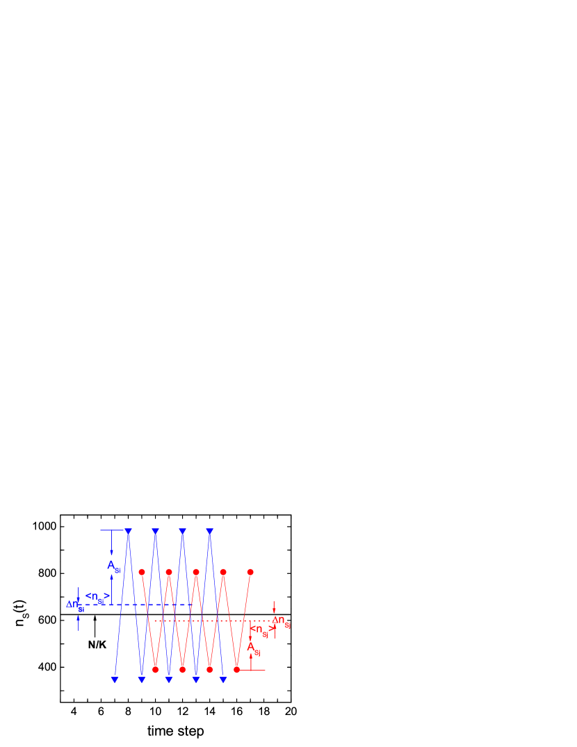
Figure 4: For the case of two groups [e.g., Fig. 1(b)], schematic illustration of time series $n_{s_{i}}$ in group $g_{1}$ (blue circles) and $n_{s_{j}}$ in group $g_{2}$ (red triangles), where various quantities such as the amplitude $A$ are labeled.

Based on the numerical observations, we can argue that the strategy grouping phenomenon is intimately related to the fluctuations in the time series $n_{s}$. Assuming the MG system is closed so that the number of agents is a constant, we have

$$k_{g_{1}}\cdot n_{s_{i}}(t)+k_{g_{2}}\cdot n_{s_{j}}(t)=N.$$ (5)

Thus, for two consecutive time steps, we have,

$$k_{g_{1}}\cdot(\langle n_{s_{i}}\rangle+A_{s_{i}})+k_{g_{2}}\cdot(\langle n_{s_{j}}\rangle-A_{s_{j}}) = N,$$

$$k_{g_{1}}\cdot(\langle n_{s_{i}}\rangle-A_{s_{i}})+k_{g_{2}}\cdot(\langle n_{s_{j}}\rangle+A_{s_{j}}) = N.$$ (6)

Substituting Eq. (4) into Eq. (6), we have

$$k_{g_{1}}\cdot(\frac{N}{k}+\Delta n_{s_{i}}+A_{s_{i}}) + k_{g_{2}}\cdot(\frac{N}{k}-\Delta n_{s_{j}}-A_{s_{j}})=N,$$

$$k_{g_{1}}\cdot(\frac{N}{k}+\Delta n_{s_{i}}-A_{s_{i}}) + k_{g_{2}}\cdot(\frac{N}{k}-\Delta n_{s_{j}}+A_{s_{j}})=N,$$

from which we obtain the relations between $A_{s_{i}}$ and $A_{s_{j}}$, $\Delta n_{s_{i}}$ and $\Delta n_{s_{j}}$ as

$$\frac{A_{s_{i}}}{A_{s_{j}}}=\frac{k_{g_{2}}}{k_{g_{1}}},\quad\frac{\Delta n_{s_{i}}}{\Delta n_{s_{j}}}=\frac{k_{g_{2}}}{k_{g_{1}}}.$$ (7)

We see that the fluctuations of the time series are closely related the grouping of the strategies.

From the definition of $\sigma^{2}_{s}$, we can write the variances of $n_{s_{i}}$ and $n_{s_{j}}$ as

$$\sigma_{s_{i}}^{2} = \frac{(A_{s_{i}}+\Delta n_{s_{i}})^{2}+(A_{s_{i}}-\Delta n_{s_{i}})^{2}}{2}=A_{s_{i}}^{2}+\Delta n_{s_{i}}^{2},$$

$$\sigma_{s_{j}}^{2} = \frac{(A_{s_{j}}-\Delta n_{s_{j}})^{2}+(A_{s_{j}}+\Delta n_{s_{i}})^{2}}{2}=A_{s_{j}}^{2}+\Delta n_{s_{j}}^{2}.$$

Using Eq. (7), we obtain

$$\frac{\sigma_{s_{i}}^{2}}{\sigma_{s_{j}}^{2}}=(\frac{k_{g_{2}}}{k_{g_{1}}})^{2}.$$ (8)

As shown in Fig. 2, the ratio of the variances of group $g_{1}$ and $g_{2}$ from the simulation agree very well with Eq. (8).

IV.2 Mean-field theory

We develop a mean-field theory to understand the fluctuation patterns of the system. To be concrete, we still treat the case of two distinct groups. Consider strategy $s_{i}$ that belongs to group $g_{1}$ and assume that $s_{i}$ is the majority strategy at time $t=t_{0}$, i.e., $n_{s_{i}}^{(0)}>N/k$. According to the mean-field approximation, at the next time step $t=t_{0}+1$, the number of agents $n_{s_{i}}^{(1)}$ choosing strategy $s_{i}$ is

$$n_{s_{i}}^{(1)} = n_{s_{i}}^{(0)}-(w_{1}+w_{2})+w_{3}$$ (9)

$$= n_{s_{i}}^{(0)}-[n_{s_{i}}^{(0)}p+n_{s_{i}}^{(0)}(1-p)m\frac{k-1}{k}]$$

$$+ (N-n_{s_{i}}^{(0)})(1-p)m\frac{1}{k},$$

where

$$w_{1} = n_{s_{i}}^{(0)}p,$$

$$w_{2} = n_{s_{i}}^{(0)}(1-p)m\frac{(k-1)}{k},$$

$$w_{3} = (N-n_{s_{i}}^{(0)})(1-p)m\frac{1}{k}.$$ (10)

Here, $w_{1}$ and $w_{2}$ together are the number of agents abandoning strategy $s_{i}$ (or the flow out of strategy $s_{i}$). That is, of the $n_{s_{i}}^{(0)}$ agents, $w_{1}$ agents will act based on local information by selecting a minority strategy different than $s_{i}$ for the next time step $t_{0}+1$. At the same time, there will be $w_{2}$ agents acting without local information by choosing randomly one of the other $k-1$ strategies. The quantity $w_{3}$ represents the flow into $s_{i}$ from the remaining $N-n_{s_{i}}^{(0)}$ agents. These agents will mutate randomly to switch their strategies to $s_{i}$ without any local information. We thus have

$$n_{s_{i}}^{(1)}=n_{s_{i}}^{(0)}(1-p)(1-m)+N(1-p)m\frac{1}{k}.$$ (11)

Suppose $n_{s_{i}}^{(1)}<N/k$. Then $s_{i}$ and the other $k_{g_{1}}-1$ strategies in $g_{1}$ are the minority strategy, and the agents selecting those strategies win the game at $t=t_{0}+1$. The time series $n_{s_{i}}^{(2)}$ at time $t_{0}+2$ can be written as

$$n_{s_{i}}^{(2)} = n_{s_{i}}^{(1)}-n_{s_{i}}^{(1)}[p\frac{(k_{g_{1}}-1)}{k_{g_{1}}}+(1-p)m\frac{(k-1)}{k}]$$ (12)

$$+ (N-n_{s_{i}}^{(1)})[p\frac{1}{k_{g_{1}}}+(1-p)m\frac{1}{k}]$$

$$= n_{s_{i}}^{(1)}-(w_{4}+w_{5})+(w_{6}+w_{7}),$$

where $w_{4}$ and $w_{5}$ stand for the flows out of strategy $s_{i}$, while $w_{6}$ and $w_{7}$ represent the flows into $s_{i}$ from those $N-n_{s_{i}}^{(0)}$ agents on other strategies. We have

$$n_{s_{i}}^{(2)}=n_{s_{i}}^{(1)}(1-p)(1-m)+N(1-p)m\frac{1}{k}+Np\frac{1}{k_{g_{1}}},$$ (13)

where $n_{s_{i}}^{(2)}$ is larger than $N/k$, $s_{i}$ and all other strategies in group $g_{1}$ will be the majority strategy again, as at time $t_{0}$. The process $n_{s_{i}}\rightarrow n_{s_{i}}^{(1)}\rightarrow n_{s_{i}}^{(2)}$ thus occurs iteratively. From Eqs. (11) and (13), we can get the number of agents for one given strategy at any time $t$. In particular, denoting $\alpha\equiv(1-p)(1-m)$, $\beta\equiv N(1-p)m/k$, and $\gamma_{g_{1}}\equiv Np/k_{g_{1}}$, we obtain the iterative dynamics for agents selecting strategy $s_{i}$ as

$$n_{s_{i}}^{(1)}=\alpha n_{s_{i}}^{(0)}+\beta,$$ (14)

$$n_{s_{i}}^{(2)}=\alpha n_{s_{i}}^{(1)}+\beta+\gamma_{g_{1}},$$

$$n_{s_{i}}^{(3)}=\alpha n_{s_{i}}^{(2)}+\beta,$$

$$\cdots\cdots\cdots\cdots\cdots$$

$$n_{s_{i}}^{(2a)}=\alpha n_{s_{i}}^{(2a-1)}+\beta+\gamma_{g_{1}},$$

$$n_{s_{i}}^{(2a+1)}=\alpha n_{s_{i}}^{(2a)}+\beta,$$

$$\cdots\cdots\cdots\cdots\cdots$$

where $a\in R$ and $n_{s_{i}}^{(t^{\prime})}$ stands for the number of agents at $t=t_{0}+t^{\prime}$. Carrying out the iterative process in Eq. (14), we obtain

$$n_{s_{i}}^{(2)}=\alpha^{2}n_{s_{i}}^{(0)}+\alpha\beta+\beta+\gamma_{g_{1}},$$

$$n_{s_{i}}^{(3)}=\alpha^{2}n_{s_{i}}^{(1)}+\alpha\beta+\alpha\gamma_{g_{1}}+\beta.$$

For the case where $n_{s}(t)$ exhibits stable oscillations, i.e., the system is in a stationary state, we have,

$$n_{s_{i}}^{(0)}=n_{s_{i}}^{(2)}=\cdots=n_{s_{i}}^{(2a)}\quad a\in R,$$

$$n_{s_{i}}^{(1)}=n_{s_{i}}^{(3)}=\cdots=n_{s_{i}}^{(2a+1)}.$$

We thus obtain the values of $n_{s_{i}}^{(2a)}$ and $n_{s_{i}}^{(2a+1)}$ as a function of the probability $p$, mutation probability $m$, and the grouping parameter $k_{g_{1}}$, and $k$:

$$n_{s_{i}}^{(2a)}=\frac{\alpha\beta+\beta+\gamma_{g_{1}}}{1-\alpha^{2}},$$

$$n_{s_{i}}^{(2a+1)}=\frac{\alpha\beta+\alpha\gamma_{g_{1}}+\beta}{1-\alpha^{2}}.$$ (15)

From $n_{s}$, we can get the expression of the amplitude of the fluctuation, the mean value $\langle{n_{s_{i}}}\rangle$, and its difference from $N/k$ as,

$$A_{s_{i}}=[n_{s_{i}}^{(2a)}-n_{s_{i}}^{(2a+1)}]/2=\frac{\gamma_{g_{1}}}{2(1+\alpha)},$$

$$\langle{n_{s_{i}}}\rangle=[n_{s_{i}}^{(2a)}+n_{s_{i}}^{(2a+1)}]/2=\frac{2\beta+\gamma_{g_{1}}}{2(1-\alpha)},$$

$$\Delta n_{s_{i}}=|\langle{n_{s_{i}}}\rangle-N/k|=|\frac{k\gamma_{g_{1}}-2Np}{2k(1-\alpha)}|=\frac{Np|k/k_{g_{1}}-2|}{2k(1-\alpha)}.$$

In the above derivation, we have assumed that $s_{i}$ belongs to group $g_{1}$, and obtained expressions of the $n_{s_{i}}$, $A_{s_{i}}$, $\langle{n_{s_{i}}}\rangle$, and $\Delta n_{s_{i}}$. Similarly, using Eq. (5), we can calculate the time series $n_{s_{j}}$, the number of agents selecting the strategy $s_{j}$ belonging to group $g_{2}$, and the corresponding characterizing quantities.

Alternatively, following the steps similar to those from Eqs. (9) to (14), we can write the recurrence formula for $n_{s_{j}}$ as

$$n_{s_{j}}^{(2a)}=\alpha n_{s_{j}}^{(2a-1)}+\beta,$$

$$n_{s_{j}}^{(2a+1)}=\alpha n_{s_{j}}^{(2a)}+\beta+\gamma_{g_{2}},$$

where $\gamma_{g_{2}}=Np/k_{g_{2}}$. For the case of stable strategy, we get the corresponding number of agents as

$$n_{s_{j}}^{(2a)}=\frac{\alpha\beta+\alpha\gamma_{g_{2}}+\beta}{1-\alpha^{2}},$$

$$n_{s_{j}}^{(2a+1)}=\frac{\alpha\beta+\beta+\gamma_{g_{2}}}{1-\alpha^{2}}.$$ (16)

We find that the values of $n_{s}$ obtained from Eq. (16) agree with those from Eq. (5) very well (derivation and data not shown). In addition, the expressions of $A_{s_{j}}$, $\langle{n_{s_{j}}}\rangle$, and $\Delta n_{s_{j}}$ are identical to those associated with $s_{i}$, with the quantity $\gamma_{g_{1}}$ replaced by $\gamma_{g_{2}}$.

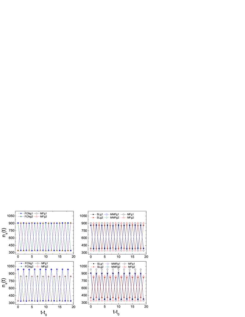
Figure 5: (Color online.) Comparison of the time series of $n_{s_{i}}$ in group $g_{1}$ (and $n_{s_{j}}$ in group $g_{2}$) from the mean-field formula [Eq. (15)] and modified mean-field formula [Eq. (18)], and from simulations. The upper and lower figures show the results for the grouping state $(8,8)$ and $(7,9)$, respectively. The left panels are the results from mean-field theory (MF) and from simulations on fully connected networks (FCN). The right panels are the results from our modified mean-field theory (MMF) and simulations on the square lattice (SL). The system parameters are $N=10000$, $k=16$, $p=0.45$, and $m=1$.

The mean-field theory is ideally suited for fully connected networks. Indeed, results from the theory and direct simulations agree with each other very well, as shown in Fig. 5. However, in real-world situations, a fully connected topology cannot be expected, and the mean-field treatment will no longer be accurate. For example, we have carried out simulations on square-lattice systems and found noticeable deviations from the mean-field prediction. To remedy this deficiency, we develop a modified mean-field analysis for MG dynamics on sparsely homogeneous networks (e.g., square lattices or random networks).

IV.3 Mean-field theory for MG dynamics on sparsely homogeneous networks

Due to the limited number of links in a typical large-scale network, it is possible for a failed agent to be surrounded by agents from the same group (who will likewise fail the game). In this case, the failed agent has no minority strategy to imitate (set $\Pi$ is empty) and thus will randomly select one strategy from the $k$ available strategies. Taking this effect into account, we can modify the mean-field approximation in Eqs. (9) and (12) as

$$n_{s_{i}}^{(1)}=n_{s_{i}}^{(0)}-(w_{1}+w_{2})+w_{3}+w_{8},$$ (17)

$$n_{s_{i}}^{(2)}=n_{s_{i}}^{(1)}-(w_{4}+w_{5})+(w_{6}+w_{7})+w_{9},$$

with the two modified terms given by

$$w_{8}=k_{g_{1}}n_{s_{i}}^{(0)}p\eta_{g_{1}}\frac{1}{k},$$

$$w_{9}=(N-k_{g_{1}}n_{s_{i}}^{(1)})p\eta_{g_{2}}(\frac{1}{k}-\frac{1}{k_{g_{1}}}),$$

where $\eta_{g_{x}}$ is the probability for one agent in group $g_{x}$ to be surrounded by agents from the same group. The quantity $w_{8}$ stands for the flow from the failed agents in group $g_{1}$ [the number is $N_{g_{1}}\equiv k_{g_{1}}n_{s_{i}}^{(0)}$], who react to the information [the number is $N_{g_{1}}p$] but with no winner surrounded to supply the optional minority strategy [the number is $N_{g_{1}}p\eta_{g}$], and thus select $s_{i}$ with probability $1/k$. The quantity $w_{9}$ represent two factors: (1) the $n_{1}=(N-k_{g_{1}}n_{s_{i}}^{(1)})p\frac{1}{k_{g_{1}}}\eta_{g_{2}}$ failed agents in group $g_{2}$ who should have flow into $s_{i}$ [i.e. $w_{6}$] but are held back because they are surrounded by agents in $g_{2}$, and (2) the failed agents in group $g_{2}$ who are surrounded by agents in $g_{2}$ and thus select $s_{i}$ with $1/k$ probability, the number of which is $n_{2}=(N-k_{g_{1}}n_{s_{i}}^{(1)})p\eta_{g_{2}}\frac{1}{k}$. Apparently, we have $w_{9}=n_{2}-n_{1}$.

From Eq. (17), we obtain

$$n^{(2a)}_{s_{i}}=\frac{\alpha^{\prime\prime}_{g_{1}}\beta+\beta+\gamma^{\prime}_{g_{1}}}{1-\alpha^{\prime}_{g_{1}}\alpha^{\prime\prime}_{g_{1}}},$$ (18)

$$n^{(2a+1)}_{s_{i}}=\frac{\alpha^{\prime}_{g_{1}}\beta+\alpha^{\prime}_{g_{1}}\gamma^{\prime}_{g_{1}}+\beta}{1-\alpha^{\prime}_{g_{1}}\alpha^{\prime\prime}_{g_{1}}},$$

$$A_{s_{i}}=\frac{(\alpha^{\prime\prime}_{g_{1}}-\alpha^{\prime}_{g_{1}})\beta+(1-\alpha^{\prime}_{g_{1}})\gamma^{\prime}_{g_{1}}}{2(1+\alpha^{\prime}_{g_{1}}\alpha^{\prime\prime})},$$

$$\langle{n_{s_{i}}}\rangle=\frac{\beta(\alpha^{\prime\prime}_{g_{1}}+\alpha^{\prime}_{g_{1}}+2)+\gamma^{\prime}_{g_{1}}(1+\alpha^{\prime}_{g_{1}})}{2(1-\alpha^{\prime}_{g_{1}}\alpha^{\prime\prime}_{g_{1}})},$$

$$\Delta n_{s_{i}}=|\frac{\beta(\alpha^{\prime}_{g_{1}}+\alpha^{\prime\prime}_{g_{1}})+\gamma^{\prime}_{g_{1}}(1+\alpha^{\prime}_{g_{1}})+2\beta}{2(1-\alpha^{\prime}_{g_{1}}\alpha^{\prime\prime}_{g_{1}})}-\frac{N}{k}|,$$

where the parameters are

$$\alpha^{\prime}_{g_{1}}=(1-p)(1-m)+\frac{k_{g_{1}}p\eta_{g_{1}}}{k},$$

$$\alpha^{\prime\prime}_{g_{1}}=(1-p)(1-m)+k_{g_{1}}p\eta_{g_{2}}(\frac{1}{k}_{g_{1}}-\frac{1}{k}),$$

$$\gamma^{\prime}_{g_{1}}=Np[\frac{1}{k_{g_{1}}}+\eta_{g_{2}}(\frac{1}{k}-\frac{1}{k_{g_{1}}})].$$

The equation set (18) represents the modified mean-field description of the time series associated with the stable strategies in the game system supported on sparsely homogeneous networks. The density of agents in $g_{x}$ is denoted by $\rho_{g_{x}}\equiv N_{g_{x}}/N$. For the case where agents from different groups are well mixed in the network, the probability for one given agent in $g_{x}$ to meet with agents in $g_{y}$ is $P_{g_{x}g_{y}}=\rho_{g_{y}}$ (for $x,y=1,2$). If the average degree of the network is $d$, the probability that one agent from $g_{x}$ is surrounded by agents from the same group is $\eta_{g_{x}}=(P_{g_{x}g_{x}})^{d}=\rho_{g_{x}}^{d}$. From the simulation on the square lattice system where each agent has $d=4$ neighbors, we observe a quite weak effect of clustering of agents in $g_{1}$ or $g_{2}$, so $\eta_{g_{x}}\approx\rho_{g_{x}}^{4}=(N_{g_{x}}/N)^{4}$. Based on the quantity $\eta_{g_{x}}$, analytic prediction of the time series in the modified mean-field (MMF) theory can be obtained, as shown in Fig. 5 for a square-lattice system. We observe a good agreement with simulation results. Simulations on homogeneous networks of different values $d$ have also been carried out, with results in good agreement with the prediction from the modified mean-field theory.

IV.4 Stability of strategy grouping states

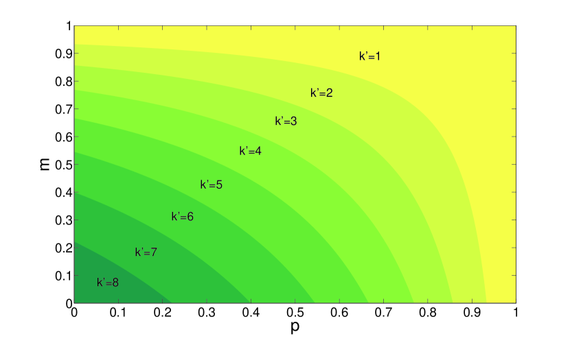
Figure 6: (Color online.) Phase diagram indicating the stability region of strategy-grouping states. The stable parameter region of one given grouping state with $k_{g_{1}}=k^{\prime}$ is at the upper right of the corresponding curve of $k^{\prime}$.

Our mean-field treatment yields formula characterizing the stable oscillations associated with the grouping state $(k_{g_{1}},k_{g_{2}})$, which include the variance ratio of the pairing groups [Eq. (8)] and time series $n_{s}$ [Eqs. (15) and (18)]. However, from the simulation result shown in Fig. 3, we see that not all the grouping states are stable in the parameter space. As $p$ is increased, the strategy-grouping state of the smaller $k_{g_{1}}$ becomes stable, and the corresponding branch appears. It is therefore useful to analyze the stability of the grouping state.

In our treatment we have assumed $n_{s_{i}}^{(0)}>N/k$ and $n_{s_{j}}^{(0)}<N/k$. Then, the necessary condition for the grouping state $(k_{g_{1}},k_{g_{2}})$ to become stable is $n_{s_{i}}^{(1)}<N/k$ and $n_{s_{j}}^{(1)}>N/k$. Using Eqs. (15) and (16), we get

$$k_{g_{1}} > \frac{k(1-m-p+pm)}{2-m-p+pm}\equiv\xi_{1}(p,m),$$ (19)

$$k_{g_{2}} < \frac{k}{2-m-p+mp}\equiv\xi_{2}(p,m),$$

where $\xi_{1}$ and $\xi_{2}$ are continuous functions of the parameters $p$ and $m$, and $\xi_{1}+\xi_{2}=k$. The two inequalities in Eq. (19) are nevertheless equivalent to each other. Figure 6 presents a phase diagram in the parameter space, where the curves of $\xi_{1}(p,m)=k^{\prime}$ for $k^{\prime}=8$, $7$, $\cdots$, $1$ are shown. The necessary condition for the strategy-grouping state with $k_{g_{1}}=k^{\prime}$ to be stable is that the the parameters $p$ and $m$ are in the upper-right region of the curve $\xi_{1}(p,m)=k^{\prime}$. For certain value of $m$, only when $p>p_{b}(m,k^{\prime})$ will the state of $k_{g_{1}}=k^{\prime}$ be stable. While the value of $p_{b}$ from simulation is different from the theoretical value $p_{b}(m,k^{\prime})$, our mean-field theory does provide a qualitative explanation for the phenomenon in Fig. 3(a), where more branches of smaller strategy-grouping states become stable as $p$ is increased.

We have also seen in Fig. 2, and Fig. 3(a) that, as $p$ approaches $1$, the bifurcated branches of different grouping state merge together. For the case of even $k$, $n_{s}$ fluctuates stably in the grouping state with $k_{g_{1}}=k_{g_{2}}=k/2$. While, for the case of odd $k$, $n_{s}$ fluctuates quasiperiodicly [see Fig. 1(c)]. Actually, the grouping state always switches between $(k_{g}+1,k_{g})$ and $(k_{g},k_{g}+1)$, with $k_{g}=(k-1)/2$. We can understand the instability and merging of grouping states from Fig. 1(c), and the schematic map in Fig. 4, as follows. As $p$ is increased to $1$, $\Delta n_{s_{i}}$ and $\Delta n_{s_{j}}$ increase and become comparable to the amplitudes $A_{s_{i}}$ and $A_{s_{j}}$, respectively. Namely, the attendances $n_{s}$ of strategies can be very close to $n_{c}=N/k$ . In case that $n_{s}$ of one strategy does not get cross $n_{c}$ because of noise, i.e., it acts as minority (or majority) strategy twice, then, the fluctuation of $n_{s}$, as well as the grouping state is changed.

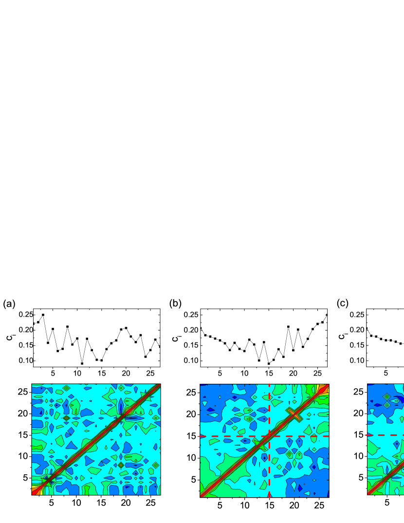
Figure 7: (Color online.) Correlation matrix of log-returns for 27 stocks in Shanghai Stock Market’s Steel Plate. (a) Original matrix C, (b) matrix $\textbf{C}^{\prime}$ ordered according to the eigenvector for the maximum eigenvalue of C, and (c) reordered matrix $\textbf{C}^{\prime\prime}$ from $\textbf{C}^{\prime}$ with respect to $c_{i}$ within each group. The $c_{i}$ values of the stocks are shown for each matrix.

V A real-world example: emergence of grouping states in financial market

The financial market is a representative multi-resource complex system, in which many stocks are available for investment. We analyze the fluctuation of the stock price from the empirical data of 27 stocks in the Shanghai Stock Market’s Steel Plate between 2007 and 2010. We regard the $27$ stocks, which are derived from the iron and steel industry, as constituting a MG system with $k=27$ resources, where the agents selecting the resources correspond to the capitals invested. This system is open in the sense that capital typically flows in and out, which is the main difference from our closed-system model. In particular, given the time series $x_{i}(t)$ of the daily closing price of stock $i$, the daily log-return is defined as $R_{i}(t)=\ln x_{i}(t)-\ln x_{i}(t-1)$. The average return of the $27$ stocks at time $t$, denoted by $\langle R_{i}(t)\rangle$, signifies a global trend of the system at $t$, which is caused by the change in the total mount of the capital in this open, 27-stock system. However, when we analyze the detrended log-returns $R_{i}^{\prime}(t)=R_{i}(t)-\langle R_{i}(t)\rangle$, the system resembles a closed system, as our model MG system. We shall demonstrate that the strategy-grouping phenomenon occurs in this real-world system.

We calculate the Pearson parameter $c_{ij}$ of each pair of the detrended log-returns $R_{i}^{\prime}(t)$ and $R_{j}^{\prime}(t)$, which leads to a $k\times k$ correlation matrix C, as shown in Fig. 7(a). In terms of the eigenvector associated with the maximum eigenvalue of matrix C, we rank the order of the stocks and obtain the matrix $\textbf{C}^{\prime}$, as shown in Fig. 7(b). The striking behavior is that the matrix is apparently divided into 4 blocks, a manifestation of the grouping phenomenon. In particular, the matrix elements $c_{ij}$ among the first 15 stocks and those among the remaining 12 stocks are generally positive, but the cross elements between stocks in the two groups are negative. It is thus quite natural to classify the first 15 stocks as belonging to group $g_{1}$ and the remaining 12 to group $g_{2}$. We can then write the matrix in a block form as

$$\textbf{C}^{\prime}=\begin{array}[]{ccc}\left(\begin{array}[]{cc}\textbf{C}_{g_{2}g_{1}}&\textbf{C}_{g_{2}g_{2}}\\ \textbf{C}_{g_{1}g_{1}}&\textbf{C}_{g_{1}g_{2}}\end{array}\right),\end{array}$$

where the elements of $\textbf{C}_{g_{1}g_{1}}$ and $\textbf{C}_{g_{2}g_{2}}$ are positive, and those of $\textbf{C}_{g_{1}g_{2}}$ and $\textbf{C}_{g_{2}g_{1}}$ are negative. The phenomenon is that the $27$-stock system has self-organized itself into a $(12,15)$ grouping state, which is a natural consequence of the MG dynamics in multi-resource complex systems.

For one given stock $i$, the mean absolute correlation is

$$c_{i}=\sum_{j=1}^{k}{|c_{ij}|}/(k-1),\qquad j\neq i.$$

This parameter reflects the weight of the stock in the system. If $c_{i}\rightarrow 0$, oscillations of stock $i$ are contained in the noise floor. In this case, there is no indication as to whether this stock belongs to group $g_{1}$ or $g_{2}$. The larger the value of $c_{i}$, the less ambiguous that the stock belongs to either one of the two groups. From the value of $c_{i}$ ranked in the same order as in $\textbf{C}^{\prime}$, we can see that the boundary of the two groups is the stock with minimum $c_{i}$. Thus $c_{i}$ can be considered as the characteristic number to distinguish different groups. We can also reorder the matrix $\textbf{C}^{\prime}$ according to $c_{i}$ within group $g_{1}$ and $g_{2}$, respectively. This leads to the matrix $\textbf{C}^{\prime\prime}$, as shown in Fig. 7(c), further demonstrating the grouping phenomenon.

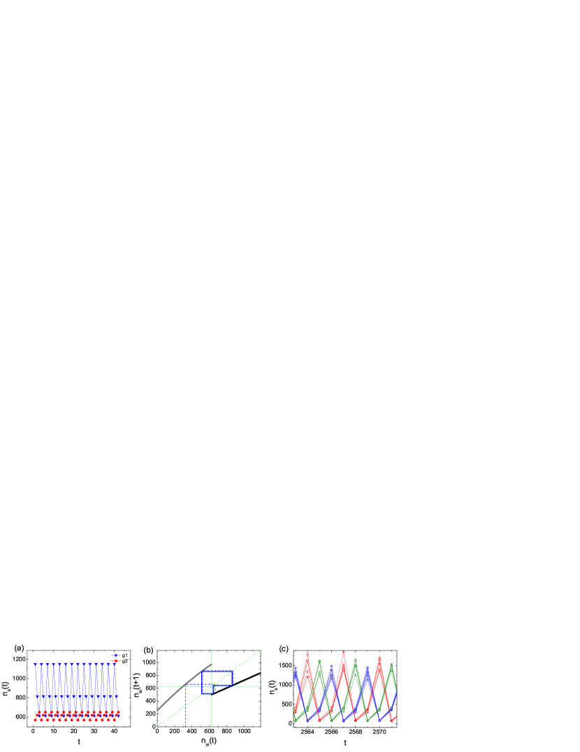
Figure 8: (Color online.) (a) The analytical time series $n_{s}(t)$ of period-tripling in the form of $2$ groups, and (b) the corresponding mapping from $n_{s_{i}}(t)$ to $n_{s_{i}}(t+1)$ for the strategy $s_{i}$ in group $g_{1}$ [see Eq. (17)]. The system is of $k=16$, $p=0.25$, $m=0.2$, and the grouping state $(k_{g_{1}},k_{g_{2}})$ is $(3,13)$, respectively. (c) The time series $n_{s}(t)$ of the stable grouping state with period-tripling in the form of $3$ groups from simulation on FCN. The system is of $k=16$, $p=0.88$, $m=1$, and the grouping state $(k_{g_{1}},k_{g_{2}},k_{g_{3}})$ is $(5,5,6)$.

VI Conclusions and discussions

Minority game, since its invention about two decades ago, has become a paradigm to study the social and economical phenomena where a large number of agents attempt to make simultaneous decision by choosing one of the available options Gintis:2009 . In the most commonly studied case of a single available resource with players’ two possible options, agents taking the minority option are the guaranteed winners. Various minority game dynamics have also received attention from the physics community due to their high relevance to a number of phenomena in statistical physics. It has become more and more common in the modern world that multiple resources are available for various social and economical systems. If the rule still holds that the winning options are minority ones, the questions that naturally arise are what type of collective behaviors can emerge and how they would evolve in the underlying complex system. Our present work aims to address these questions computationally and analytically.

The main contribution and findings of this paper are the following. Firstly, we have constructed a class of spatially extended systems in which any agent interacts with a finite but fixed number of neighbors and can choose either to follow the minority strategy based on information about the neighboring states or to select one randomly from a set of available strategies. The probability to follow the local minority strategy, or the probability of minority preference, is a key parameter determining the dynamics of the underlying complex system. Secondly, we have carried out extensive numerical simulations and discovered the emergence of a striking collective behavior: as the minority-preference probability is increased through a critical value, the set of available strategies/resources spontaneously break into pairs of groups, where the strategies in the same group are associated with a specific fluctuating behavior of attendance. This phenomenon of strategy-grouping is completely self-organized, which we conjecture is the hallmark of MG dynamics with multiple resources. Thirdly, we have developed a mean-field theory to explain and predict the emergence and evolution of the strategy-grouping states, with good agreement with the numerics. Fourthly, we have examined a real-world system of a relatively small-scale stock-trading system, and found unequivocal evidence of the grouping phenomenon. Our results suggest grouping of resources as a fundamental type of collective dynamics in multiple-resource MG systems. Other real-world systems for which our model is applicable include, e.g., hedge-fund portfolios in financial systems, routing issues in computer networks and urban traffic systems. We expect our model and findings to be not only relevant with statistical-physical systems, but also important to a host of social, economical, and political systems.

Additionally, the double-grouping (or paired grouping) period-doubling like bifurcation are not the exclusive mode for the grouping of resources. We have also observed the period$-3$ double-grouping [see Fig. 8(a)(b)], and the period$-3$ triplet-grouping bifurcation phenomena [see Fig. 8(c)]. Further research about these phenomena are of great interest and is valuable for the understanding of chaotic and bifurcation in social systems.

VII Acknowledgement

ZGH thanks Prof. Matteo Marsili for helpful discussions. This work was partially supported by the NSF of China (Grant Nos. 10905026, 10905027, 11005053, and 11135001), SRFDP No. 20090211120030, FRFCU No. lzujbky-2010-73, Lanzhou DSTP No. 2010-1-129. YCL was supported by AFOSR under Grant No. FA9550-10-1-0083.

References

- (1) W. Brian Arthur, Inductive Reasoning and Bounded Rationality, Ame. Econo. Rev. 84, 406 (1994).
- (2) H. Gintis, Game Theory Evolving (Princeton University Press, Princeton, 2009).
- (3) D. Challet and Y.-C. Zhang, Emergence of Cooperation and Organization in an Evolutionary Game, Physica A 246, 407 (1997).
- (4) D. Challet and M. Marsili, Phase Transition and Symmetry Breaking in the Minority Game, Phys. Rev. E 60, R6271 (1999).
- (5) D. Challet, M. Marsili and R. Zecchina, Statistical Mechanics of Systems with Heterogeneous Agents: Minority Games, Phys. Rev. Lett. 84, 1824 (2000).
- (6) A. De Martino, M. Marsili and R. Mulet, Adaptive Drivers in a Model of Urban Traffic, Europhys. Lett. 65, 283 (2004).
- (7) C. Borghesi, M. Marsili and S. Miccichè, Emergence of Time-horizon Invariant Correlation Structure in Financial Returns by Subtraction of the Market Mode, Phys. Rev. E 76, 026104 (2007).
- (8) R. Savit, R. Manuca, and R. Riolo, Adaptive Competition, Market Efficiency, and Phase Transitions, Phys. Rev. Lett. 82, 2203 (1999).
- (9) M. Paczuski, K. E. Bassler and A. Corral, Self-Organized Networks of Competing Boolean Agents, Phys. Rev. Lett. 84, 3185 (2000).
- (10) T. Zhou, B.-H. Wang, P.-L. Zhou, C.-X. Yang and J. Liu, Self-organized Boolean Game on Networks, Phys. Rev. E 72, 046139 (2005).
- (11) V.M. Eguiluz and M.G. Zimmermann, Transmission of Information and Herd Behavior: An Application to Financial Markets , Phys. Rev. Lett. 85, 5659 (2000).
- (12) T. Kalinowski, H.-J. Schulz and M. Birese, Cooperation in the Minority Game with Local Information, Physica A 277, 502 (2000).
- (13) F. Slanina, Harms and Benefits from Social Imitation, Physica A 299, 334 (2000).
- (14) M. Anghel, Z. Toroczkai, K. E. Bassler and G. Korniss, Competition-Driven Network Dynamics: Emergence of a Scale-Free Leadership Structure and Collective Efficiency, Phys. Rev. Lett. 92, 058701 (2004).
- (15) T. S. Lo, H. Y. Chan, P. M. Hui, and N. F. Johnson, Theory of Networked Minority Game Based on Strategy Pattern Dynamics, Phys. Rev. E 70, 056102 (2004).
- (16) T. S. Lo, K. P. Chan, P. M. Hui and N. F. Johnson, Theory of Enhanced Performance Emerging in a Sparsely Connected Competitive Population, Phys. Rev. E 71, 050101(R) (2005).
- (17) N. F. Johnson, M. Hart, and P. M. Hui, Crowd Effects and Volatility in Markets with Competing Agents, Physica A 269, 1 (1999).
- (18) M. Hart, P. Jefferies, N. F. Johnson and P. M. Hui, Crowd-Anticrowd Theory of the Minority Game, Physica A 298, 537 (2001).
- (19) D. Challet, A. De Martino and M. Marsili, Dynamical Instabilities in a Simple Minority Game with Discounting, J. Stat. Mech. (2008) L04004.
- (20) G. Bianconi, A. De Martino, F.F. Ferreira, M. Marsili, Multi-Asset Minority Games, Quant. Finance, 8(3):225-231, 2008.
- (21) Y. B. Xie and B. H. Wang, C.-K. Hu and T. Zhou, Global Optimization of Minority Game by Intelligent Agents, Eur. Phys. J. B 47, 587 (2005).
- (22) L.-X. Zhong, D. F. Zheng, B. Zheng, and P. M. Hui, Effects of Contrarians in the Minority Game, Phys. Rev. E 72, 026134 (2005).
- (23) E. Moro, The Minority Game: an Introductory Guide, in Advances in Condensed Matter and Statistical Physics, ed. by E. Korutcheva and R. Cuerno (Nova Science Publishers, Inc., 2004).
- (24) D. Challet, M. Marsili and Y.-C. Zhang, Minority Games (Oxford University Press, Oxford, 2005).
- (25) C. H. Yeung and Y.-C. Zhang, Minority Games, arXiv:0811.1479v2 (2008).