Characterizing Low-Mass Binaries From Observation of Long Time-scale Caustic-crossing Gravitational Microlensing Events

Abstract

Despite astrophysical importance of binary star systems, detections are limited to those located in small ranges of separations, distances, and masses and thus it is necessary to use a variety of observational techniques for a complete view of stellar multiplicity across a broad range of physical parameters. In this paper, we report the detections and measurements of 2 binaries discovered from observations of microlensing events MOA-2011-BLG-090 and OGLE-2011-BLG-0417. Determinations of the binary masses are possible by simultaneously measuring the Einstein radius and the lens parallax. The measured masses of the binary components are 0.43 $M_{\odot}$ and 0.39 $M_{\odot}$ for MOA-2011-BLG-090 and 0.57 $M_{\odot}$ and 0.17 $M_{\odot}$ for OGLE-2011-BLG-0417 and thus both lens components of MOA-2011-BLG-090 and one component of OGLE-2011-BLG-0417 are M dwarfs, demonstrating the usefulness of microlensing in detecting binaries composed of low-mass components. From modeling of the light curves considering full Keplerian motion of the lens, we also measure the orbital parameters of the binaries. The blended light of OGLE-2011-BLG-0417 comes very likely from the lens itself, making it possible to check the microlensing orbital solution by follow-up radial-velocity observation. For both events, the caustic-crossing parts of the light curves, which are critical for determining the physical lens parameters, were resolved by high-cadence survey observations and thus it is expected that the number of microlensing binaries with measured physical parameters will increase in the future.

1. Introduction

Binary star systems are of astrophysical importance for various reasons. First, they compose an important portion of stars in the Galaxy (Abt & Levy, 1976; Abt, 1983; Duquennoy & Mayor, 1991) and thus theories about stellar formation and evolution should account for the binary nature of stars. Second, binary stars allow us to directly measure the masses of their component stars. The determined masses in turn allow other stellar parameters, such as radius and density, to be indirectly estimated. These physical parameters help us to understand the processes by which binary stars form (Goodwin et al., 2007; Burgasser et al., 2007). In particular, the separation and mass of a binary system tell us about the amount of angular momentum in the system. Because it is a conserved quantity, binaries with measured angular momentum give us important clues about the conditions under which the stars were formed.

Despite the importance, broad ranges of separations, distances, and component masses make it hard to detect and measure all binaries. Nearby systems with wide separations may be directly resolved using high-resolution imaging, while systems with small separations can be detected as eclipsing or spectroscopic binaries. However, binaries with intermediate separations are difficult to be detected by the conventional methods. In addition, it is difficult to detect binaries if they are located at large distances or either of the binary components is faint. As a result, samples are restricted to binaries in the solar neighborhood and are not complete down to low-mass stars. For a complete view of stellar multiplicity across a broad range of physical parameters, therefore, it is necessary to use a variety of observational techniques.

Gravitational microlensing can provide a complementary method that can detect and measure binaries that are difficult to be detected by other methods. Microlensing occurs when an astronomical object is closely aligned with a background star. The gravity of the intervening object (lens) causes deflection of the light from the background star (source), resulting in the brightening of the source star. If the lens is a single star, the light curve of the source star brightness is characterized by smooth rising and fall. However, if the lens is a binary, the light curve can be dramatically different, particularly for caustic-crossing events, which exhibit strong spikes in the light curve. Among caustic-crossing binary-lens events, those with long time scales are of special importance because it is often possible to determine the physical parameters of lenses (see more details in section 2). The binary separations for which caustic crossings are likely to occur are in the range of order AU, for which binaries are difficult to be detected by other methods. In addition, due to the nature of the lensing phenomenon that occurs regardless of the lens brightness, microlensing can provide an important channel to study binaries composed of low-mass stars. Furthermore, most microlensing binaries are located at distances of order kpc and thus microlensing can expand the current binary sample throughout the Galaxy.

In this paper, we report the detections and measurements of 2 binaries discovered from observations of long time-scale caustic-crossing binary microlensing events MOA-2011-BLG-090 and OGLE-2011-BLG-0417. In §2, we describe the basic physics of binary lensing and the method to determine the physical parameters of binary lenses. In §3, we describe the choice of sample, observations of the events, and data reduction. In §4, we describe the procedure of modeling the observed light curves. In §5, we present the results from the analysis. We discuss about the findings and conclude in §6.

2. LONG TIME-SCALE CAUSTIC-CROSSING EVENTS

For a general lensing event, where a single star causes the brightening of a background source star, the magnification of the source star flux depends only on the projected separation between the source and the lens as

$$A={u^{2}+2\over u\sqrt{u^{2}+4}},$$ (1)

where the separation $u$ is normalized in units of the angular Einstein radius of the lens, $\theta_{\rm E}$. For a uniform change of the lens-source separation, the light curve of a single-lens event is characterized by a smooth and symmetric shape. The normalized lens-source separation is related to the lensing parameters by

$$u=\left[\left({t-t_{0}}\over{t_{\rm E}}\right)^{2}+u_{0}^{2}\right]^{1/2},$$ (2)

where $t_{\rm E}$ represents the time scale for the lens to cross the Einstein radius (Einstein time scale), $t_{0}$ is the time of the closest lens-source approach, and $u_{0}$ is the lens-source separation at that moment. Among these lensing parameters $t_{0}$, $t_{\rm E}$, and $u_{0}$, the only quantity related to the physical parameters of the lens is the Einstein time scale. However, it results from the combination of the lens mass, distance, and transverse speed of the relative lens-source motion and thus the information about the lens from the time scale is highly degenerate.

When gravitational lensing is caused by a binary, the gravitational field is asymmetric and the resulting light curves can be dramatically different from that of a single lensing event (Mao & Paczyński, 1991). The most prominent feature of binary lensing that differentiates it from single lensing is a caustic. A set of caustics form a boundary of an envelope of rays as a curve of concentrated light. The gradient of magnification around the caustic is very large. As a result, the light curve of an event produced by the crossing of a source star over the caustic formed by a binary lens is characterized by sharp spikes occurring at the time of caustic crossings.

Caustic-crossing binary-lens events are useful because it is often possible to measure an additional lensing parameter appearing in the expression of the Einstein radius. This is possible because the caustic-crossing part of the light curve appears to be different for events associated with source stars of different sizes (Dominik, 1995; Gaudi & Gould, 1999; Gaudi & Petters, 2002; Pejcha & Heyrovský, 2009). By measuring the deviation caused by this finite-source effect, it is possible to measure the source radius in units of the Einstein radius, $\rho_{\star}$ (normalized source radius). Then, combined with the information about the source angular size, $\theta_{\star}$, the Einstein radius is determined as $\theta_{\rm E}=\theta_{\star}/\rho_{\star}$. The Einstein radius is related to the mass, $M$, and distance to the lens, $D_{\rm L}$, by

$$\theta_{\rm E}=(\kappa M\pi_{\rm rel})^{1/2};\qquad\pi_{\rm rel}={\rm AU}\left({1\over D_{\rm L}}-{1\over D_{\rm S}}\right),$$ (3)

where $\kappa=4G/({c^{2}}{\rm AU})$, $D_{\rm S}$ is the distance to the source, and $\pi_{\rm rel}$ represents the relative lens-source proper motion. Unlike the Einstein time scale, the Einstein radius does not depend on the transverse speed of the lens-source motion and thus the physical parameters are less degenerate compared to the Einstein time scale.

Among caustic-crossing events, those with long time scales are of special interest because it is possible to completely resolve the degeneracy of the lens parameters and thus uniquely determine the mass and distance to the lens. This is possible because an additional lensing parameter of the lens parallax can be measured for these events. The lens parallax is defined as the ratio of Earth’s orbit, i.e. 1 AU, to the physical Einstein radius, $r_{\rm E}=D_{\rm L}\theta_{\rm E}$, projected on the observer plane, i.e.

$$\pi_{\rm E}={\pi_{\rm rel}\over\theta_{\rm E}}.$$ (4)

With simultaneous measurements of the Einstein radius and the lens parallax, the mass and distance to the lens are uniquely determined as

$$M={\theta_{\rm E}\over\kappa\pi_{\rm E}}$$ (5)

and

$$D_{\rm L}={{\rm AU}\over\pi_{\rm E}\theta_{\rm E}+\pi_{\rm S}};\qquad\pi_{\rm S}={{\rm AU}\over D_{\rm S}},$$ (6)

respectively (Gould, 2000). The lens parallax is measured by analyzing deviations in lensing light curves caused by the deviation of the relative lens-source motion from a rectilinear one due to the change of the observer’s position induced by the orbital motion of the Earth around the Sun (Gould, 1992; Refsdal, 1966). This deviation becomes important for long time-scale events, which endure for a significant fraction of the orbital motion of the Earth. Therefore, the probability of measuring the lens parallax is high for long time-scale events.

3. SAMPLE AND OBSERVATIONS

We searched for long time-scale caustic-crossing binary events among lensing events discovered in the 2011 microlensing observation season. We selected events to be analyzed based on the following criteria.

1. The overall light curve was well covered with good photometry.

2. At least one of caustic crossings was well resolved for the Einstein radius measurement.

3. The time scale of an event should be long enough for the lens parallax measurement.

From this search, we found 2 events of MOA-2011-BLG-090 and OGLE-2011-BLG-0417. Besides these events, there exist several other long time-scale caustic-crossing events, including MOA-2011-BLG-034, OGLE-2011-BLG-0307/MOA-2011-BLG-241, and MOA-2011-BLG-358/OGLE-2011-BLG-1132. We did not include MOA-2011-BLG-034 and MOA-2011-BLG-358/OGLE-2011-BLG-1132 in our analysis list because the coverage and photometry of the events are not good enough to determine the physical lens parameters by measuring subtle second-order effects in the lensing light curve. For OGLE-2011-BLG-0307/MOA-2011-BLG-241, the signal of the parallax effect was not strong enough to securely measure the physical parameters of the lens.

Table 1Telescopes

event	telescope
MOA-2011-BLG-090	MOA MOA-II 1.8 m, New Zealand
	OGLE Warsaw 1.3 m, Chile
	$\mu$FUN CTIO/SMARTS2 1.3 m, Chile
	$\mu$FUN PEST 0.3 m, Australia
	MiNDSTEp Danish 1.54 m, Chile
	RoboNet FTS 2.0 m, Australia
OGLE-2011-BLG-0417	OGLE Warsaw 1.3 m, Chile
	$\mu$FUN CTIO/SMARTS2 1.3 m, Chile
	$\mu$FUN Auckland 0.4 m, New Zealand
	$\mu$FUN FCO 0.36 m, New Zealand
	$\mu$FUN Kumeu 0.36 m, New Zealand
	$\mu$FUN OPD 0.6 m, Brazil
	PLANET Canopus 1.0 m, Australia
	PLANET SAAO 1.0 m, South Africa
	MiNDSTEp Danish 1.54 m, Chile
	RoboNet FTN 2.0 m, Hawaii
	RoboNet LT 2.0 m, Spain

The events MOA-2011-BLG-090 and OGLE-2011-BLG-0417 were observed by the microlensing experiments that are being conducted toward Galactic bulge fields by 6 different groups including MOA, OGLE, $\mu$FUN, PLANET, RoboNet, and MiNDSTEp. Among them, the MOA and OGLE collaborations are conducting survey observations for which the primary goal is to detect a maximum number of lensing events by monitoring a large area of sky. The $\mu$FUN, PLANET, RoboNet, and MiNDSTEp groups are conducting follow-up observations of events detected from survey observations. The events were observed by using 12 telescopes located in 3 different continents in the Southern Hemisphere. In Table 1, we list the telescopes used for the observation.

Reduction of the data was conducted by using photometry codes developed by the individual groups. The OGLE and MOA data were reduced by photometry codes developed by Udalski (2003) and Bond et al. (2001), respectively, which are based on the Difference Image Analysis method (Alard & Lupton, 1998). The $\mu$FUN data were processed using a pipeline based on the DoPHOT software (Schechter et al., 1993). For PLANET and MiNDSTEp data, a pipeline based on the pySIS software (Albrow et al., 2009) is used. For RoboNet data, the DanDIA pipeline (Bramich, 2008) is used.

To standardize error bars of data estimated from different observatories, we re-scaled them so that $\chi^{2}$ per degree of freedom becomes unity for the data set of each observatory, where $\chi^{2}$ is computed based on the best-fit model. For the data sets used for modeling, we eliminate data points with very large photometric uncertainties and those lying beyond $3\sigma$ from the best-fit model.

We present the light curves of events in Figure 1 and 2. To be noted is that the overall light curves including caustic crossings of both events are well covered by survey observations. This demonstrates that the observational cadence of survey experiments is now high enough to characterize lensing events based on their own data. The parts of light curves with 2455880 ¡ HJD ¡ 2455960 were not covered because the Galactic bulge field could not be observed. Although not included in the selection criteria, both events showed a common bump to those involved with caustic crossings: at HJD$\sim$2455655 for MOA-2011-BLG-090 and at HJD$\sim$2455800 for OGLE-2011-BLG-0417. These bumps were produced during the approach of the source trajectory close to a cusp of a caustic. An & Gould (2001) pointed out that such triple-peak features help to better measure the lens parallax.

4. MODELING LIGHT CURVES

In modeling the light curve of each event, we search for a solution of lensing parameters that best characterizes the observed light curve. Describing the basic feature of a binary-lens light curve requires 6 parameters including the 3 single-lensing parameters $t_{0}$, $u_{0}$, and $t_{\rm E}$. The 3 additional binary-lensing parameters include the mass ratio between the lens components, $q$, the projected separation in units of the Einstein radius, $s_{\perp}$, and the angle between the source trajectory and the binary axis, $\alpha$ (trajectory angle).

In addition to the basic binary lensing parameters, it is required to include additional parameters to precisely describe detailed features caused by various second-order effects. The first such effect is related to the finite size of the source star. This finite-source effect becomes important when the source is located at a position where the gradient of magnification is very high and thus different parts of the source surface experience different amounts of magnification. For binary-lens events, this happens when the source approaches or crosses the caustic around which the gradient of magnification is very high. To describe the light curve variation caused by the finite-source effect, it is necessary to include an additional parameter of the normalized source radius, $\rho_{\star}$.

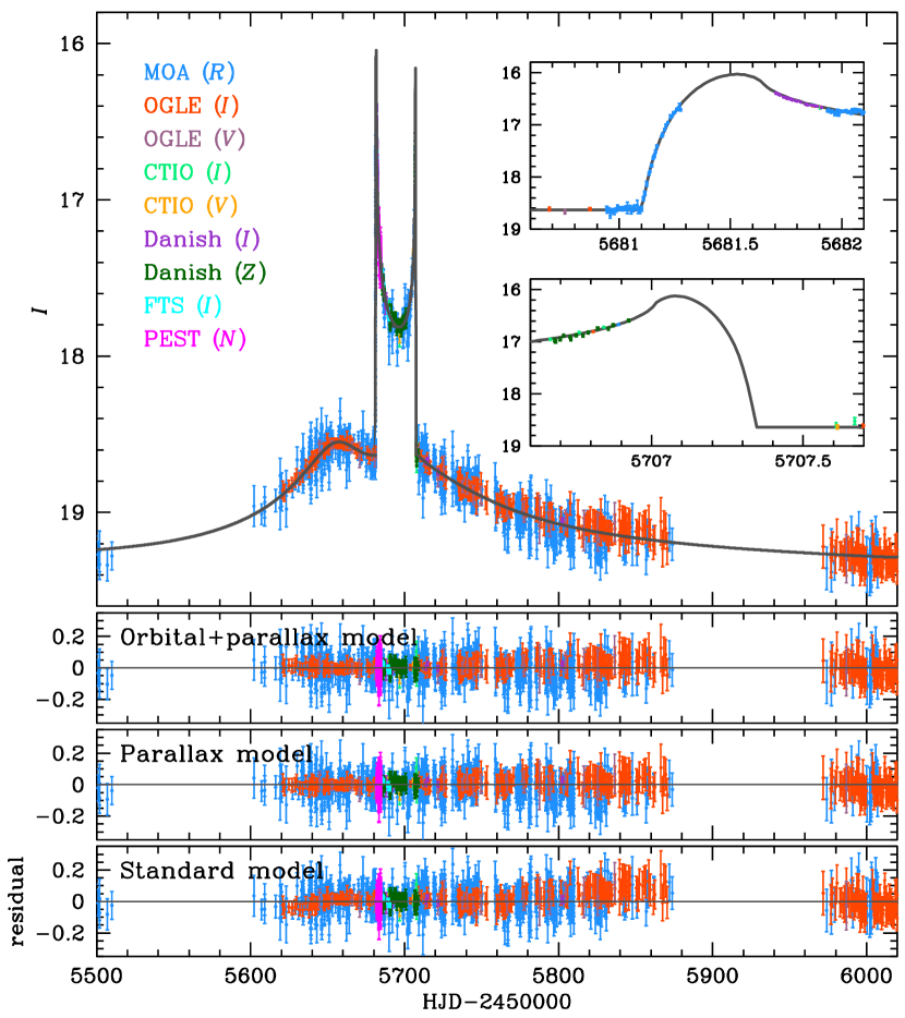
Figure 1.— Light curve of MOA-2011-BLG-090. The notation in the parentheses after each observatory denotes the passband of observation, where $N$ denotes that no filter was used. The insets in the upper panel show the enlargement of the caustic crossing parts of the light curve. The lower 3 panels show the residuals from the 3 tested models. See section 4 for more details about the individual models.

For long time-scale events, such as those analyzed in this work, it is required to additionally consider the parallax effect. Consideration of the parallax effect in modeling requires to include 2 additional parameters $\pi_{{\rm E},N}$, and $\pi_{{\rm E},E}$, which represent the two components of the lens parallax vector $\mbox{\boldmath$\pi$}_{\rm E}$ projected on the sky along the north and east equatorial coordinates, respectively. The direction of the lens parallax vector corresponds to the relative lens-source relative motion in the frame of the Earth at a specific time of the event. The size of the vector corresponds to the ratio of the Earth’s orbit to the Einstein radius projected on the observer’s plane, i.e. $\pi_{\rm E}={\rm AU}/[r_{\rm E}D_{\rm S}/(D_{\rm S}-D_{\rm L})]$, where $r_{\rm E}=D_{\rm L}\theta_{\rm E}$ is the physical size of the Einstein radius.

Another effect to be considered for long time-scale events is the orbital motion of the lens (Dominik, 1998; Ioka et al., 1999; Albrow et al., 2000; Penny et al., 2011; Shin et al., 2011; Skowron et al., 2011). The lens orbital motion affects lensing light curves in two different ways. First, it causes to change the binary separation and thus the magnification pattern. Second, it also causes the binary axis to rotate with respect to the source trajectory. In order to fully account for the lens orbital motion, 4 additional parameters are needed. The first two of these parameters are $ds_{\perp}/dt$ and $d\alpha/dt$, which represent the change rates of the projected binary separation and the trajectory angle, respectively. The other two orbital parameters are $s_{\parallel}$ and $ds_{\parallel}/dt$, where $s_{\parallel}$ represents the line-of-sight separation between the binary components in units of $\theta_{\rm E}$ and $ds_{\parallel}/dt$ represents its rate of change. For a full description of the orbital lensing parameters, see the summary in the Appendix of Skowron et al. (2011). The deviation in a lensing light curve affected by the orbital effect is smooth and long lasting and thus is similar to the deviation induced by the parallax effect. This implies that if the orbital effect is not considered, the measured lens parallax and the resulting lens parameters might be erroneous. Therefore, considering the orbital effect is important not only for constraining the orbital motion of the lens but also for precisely determining the physical parameters of the lens.

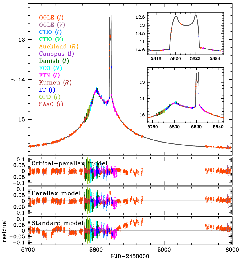
Figure 2.— Light curve of OGLE-2011-BLG-0417. Notations are same as in Fig 1.

With all these parameters, we test three different models. In the first model, we fit the light curve with standard binary lensing parameters considering the finite-source effect (standard model). In the second model, we additionally consider the parallax effect (parallax model). Finally, we take the orbital effect into consideration as well (orbital model). When the source trajectory is a straight line, the two light curves resulting from source trajectories with positive ($+u_{0}$) and negative ($-u_{0}$) impact parameters are identical due to the symmetry of the magnification pattern with respect to the binary axis. When either the parallax or the orbital effect is considered, on the other hand, the source trajectory deviates from a straight line and thus the light curves with $+u_{0}$ and $-u_{0}$ are different from each other. We, therefore, consider both the $+u_{0}$ and $-u_{0}$ cases for each of the models considering the parallax and orbital effects.

In modeling, the best-fit solution is obtained by minimizing $\chi^{2}$ in the parameter space. We conduct this in 3 stages. In the first stage, grid searches are conducted over the space of a subset of parameters and the remaining parameters are searched by using a downhill approach (Dong et al., 2006). We then identify local minima in the grid-parameter space by inspecting the $\chi^{2}$ distribution. In the second stage, we investigate the individual local minima by allowing the grid parameters to vary and find the exact location of each local minimum. In the final stage, we choose the best-fit solution by comparing $\chi^{2}$ values of the individual local minima. This multiple stage procedure is needed for thorough investigation of possible degeneracy of solutions. We choose of $s_{\perp}$, $q$, and $\alpha$ as the grid parameters because they are related to the light curve features in a complex way such that a small change in the values of the parameters can lead to dramatic changes in the resulting light curve. On the other hand, the other parameters are more directly related to the light curve features and thus they are searched for by using a downhill approach. For the $\chi^{2}$ minimization in the downhill approach, we use the Markov Chain Monte Carlo (MCMC) method. Once a solution of the parameters is found, we estimate the uncertainties of the individual parameters based on the chain of solutions obtained from MCMC runs.

Figure 3.— The caustic geometries and source trajectories of the best-fit models for MOA-2011-BLG-090 (left panel) and OGLE-2011-BLG-0417 (right panel). The small closed figures composed of concave curves represent the caustics. The small open circles represent the lens positions. We note that the lens positions and the resulting caustic vary in time due to the orbital motion of the lens. We mark 2 sets of lens positions and caustics at 2 different times of $t_{1}$ and $t_{2}$. We also note that the source trajectory, the curve with an arrow, is curved due to the combination of the parallax and orbital effects. The source trajectory is presented so that the binary axis is set along the horizontal axis. The dashed circles represent the Einstein rings corresponding to the total mass of the binary lenses.

Table 2Limb-darkening coefficients

quantity	MOA-2011-BLG-090	OGLE-2011-BLG-0417
$\Gamma_{V}$	0.52	0.71
$\Gamma_{R}$	0.45	0.61
$\Gamma_{I}$	0.37	0.51
source type	FV	KIII
$T_{\rm eff}$ (K)	6650	4660
$v_{\rm turb}$ ($\rm km\ s^{-1}$)	2	2
$\log{g}$ ($\rm cm\ s^{-2}$)	4.5	2.5

To compute lensing magnifications affected by the finite-source effect, we use the ray-shooting method. (Schneider & Weiss, 1986; Kayser et al., 1986; Wambsganss, 1997). In this method, rays are uniformly shot from the image plane, bent according to the lens equation, and land on the source plane. Then, a finite magnification is computed by comparing the number densities of rays on the image and source planes. Precise computation of finite magnifications by using this numerical technique requires a large number of rays and thus demands heavy computation. To minimize computation, we limit finite-magnification computation by using the ray-shooting method only when the lens is very close to caustics. In the adjacent region, we use an analytic hexadecapole approximation (Pejcha & Heyrovský, 2009; Gould, 2008). In the region with large enough distances from caustics, we use a point-source magnifications.

Figure 4.— OGLE color-magnitude diagrams of stars in the fields where the lensing events MOA-2011-BLG-090 (left panel) and OGLE-2011-BLG-0417 (right panel) occurred. The red and blue dots represent the centroid of the giant clump and the location of the source star for each event, respectively. For OGLE-2011-BLG-0417, we also mark the position of the blended star.

In the finite magnification computation, we consider the variation of the magnification caused by the limb-darkening of the source star’s surface. We model the surface brightness profile of a source star as

$$S_{\lambda}={F_{\lambda}\over{\pi{\theta_{\star}}^{2}}}\left[1-\Gamma_{\lambda}\left(1-{3\over{2}}\cos\psi\right)\right],$$ (7)

where $\Gamma_{\lambda}$ is the linear limb-darkening coefficients, $F_{\lambda}$ is the source star flux, and $\psi$ is the angle between the normal to the source star’s surface and the line of sight toward the star. The limb-darkening coefficients are set based the source type that is determined on the basis of the color and magnitude of the source. In Table 2, we present the used limb-darkening coefficients, the corresponding source types, and the measured de-reddened color along with the assumed values of the effective temperature, $T_{\rm eff}$, the surface turbulence velocity, $v_{\rm turb}$, and the surface gravity, $\log{g}$. For both events, we assume a solar metallicity.

5. RESULTS

In Table 3, we present the solutions of parameters for the tested models. The best-fit model light curves are drawn on the top of the observed light curves in Figures 1 and 2. In Figure 3, we present the geometry of the lens systems where the source trajectory with respect to the caustic and the locations of the lens components are marked. We note that the source trajectories are curved due to the combination of the parallax and orbital effects. We also note that the positions of the lens components and the corresponding caustics change in time due to the orbital motion and thus we present caustics at 2 different moments that are marked in Figure 3. These moments correspond to those of characteristic features on the light curve such as the peak involved during a cusp approach or a caustic crossing. To better show the differences in the fit between different models, we present the residuals of data from the best-fits of the individual models. For a close-up view of the caustic-crossing parts of the light curves, we also present enlargement of the light curve.

For both events, the parallax and orbital effects are detected with significant statistical confidence levels. It is found that inclusion of the second-order effects of the parallax and orbital motions improves the fits with $\Delta\chi^{2}=571$ and $2680$ for MOA-2011-BLG-090 and OGLE-2011-BLG-0417, respectively. To be noted is that the orbital effect is considerable for OGLE-2011-BLG-0417 and thus the difference between the values of the lens parallax measured with ($\pi_{\rm E}=0.40$) and without ($\pi_{\rm E}=0.17$) considering the orbital effect is substantial. Since the lens parallax is directly related to the physical parameters of the lens, this implies that considering the orbital motion of the binary lens is important for the accurate measurement of the lens parallax and thus the physical parameters.

Table 3Lensing Parameters

parameters	MOA-2011-BLG-090			OGLE-2011-BLG-0417
	model			model
	standard	parallax	orbital+parallax	standard	parallax	orbital+parallax
$\chi^{2}/{\rm dof}$	5207/5164	4718/5162	4636/5158	4415/2627	2391/2625	1735/2621
$t_{0}$ (HJD’)	5688.331$\pm$0.121	5691.563$\pm$0.187	5690.409$\pm$0.110	5817.302$\pm$0.018	5815.867$\pm$0.030	5813.306$\pm$0.059
$u_{0}$	0.3307$\pm$0.0038	-0.0613$\pm$0.0008	-0.0785$\pm$0.0005	0.1125$\pm$0.0001	-0.0971$\pm$0.0003	-0.0992$\pm$0.0005
$t_{\rm E}$ (days)	94.10$\pm$0.71	279.88$\pm$0.27	220.40$\pm$0.21	60.74$\pm$0.08	79.59$\pm$0.36	92.26$\pm$0.37
$s_{\perp}$	0.981$\pm$0.002	0.536$\pm$0.002	0.606$\pm$0.001	0.601$\pm$0.001	0.574$\pm$0.001	0.577$\pm$0.001
$q$	0.611$\pm$0.005	1.108$\pm$0.026	0.892$\pm$0.014	0.402$\pm$0.002	0.287$\pm$0.002	0.292$\pm$0.002
$\alpha$ (rad)	-0.181$\pm$0.004	0.373$\pm$0.005	0.317$\pm$0.006	1.030$\pm$0.002	-0.951$\pm$0.002	-0.850$\pm$0.004
$\rho_{\star}$ ($10^{-3}$)	2.89$\pm$0.03	0.54$\pm$0.01	0.78$\pm$0.01	3.17$\pm$0.01	2.38$\pm$0.02	2.29$\pm$0.02
$\pi_{{\rm E},N}$	–	0.205$\pm$0.003	0.159$\pm$0.003	–	0.125$\pm$0.004	0.375$\pm$0.015
$\pi_{{\rm E},E}$	–	-0.071$\pm$0.005	-0.022$\pm$0.004	–	-0.111$\pm$0.005	-0.133$\pm$0.003
$ds_{\perp}/dt$ (${\rm yr}^{-1}$)	–	–	-0.031$\pm$0.007	–	–	1.314$\pm$0.023
$d\alpha/dt$ (${\rm yr}^{-1}$)	–	–	1.066$\pm$0.005	–	–	1.168$\pm$0.076
$s_{\parallel}$	–	–	0.137$\pm$0.008	–	–	0.467$\pm$0.020
$ds_{\parallel}/dt$ (${\rm yr}^{-1}$)	–	–	-0.784$\pm$0.008	–	–	-0.192$\pm$0.036

Note. — HJD’=HJD-2450000.

Table 4Physical Lens Parameters

parameter	MOA-2011-BLG-090	OGLE-2011-BLG-0417
$M_{\rm tot}$ ($M_{\odot}$)	0.82$\pm$0.02	0.74$\pm$0.03
$M_{\rm 1}$ ($M_{\odot}$)	0.43$\pm$0.01	0.57$\pm$0.02
$M_{\rm 2}$ ($M_{\odot}$)	0.39$\pm$0.01	0.17$\pm$0.01
$\theta_{\rm E}$ (mas)	1.06$\pm$0.01	2.44$\pm$0.02
$\mu$ (mas yr-1)	1.76$\pm$0.02	9.66$\pm$0.07
$D_{\rm L}$ (kpc)	3.26$\pm$0.05	0.89$\pm$0.03
$a$ (AU)	1.79$\pm$0.02	1.15$\pm$0.04
$P$ (yr)	2.65$\pm$0.04	1.44$\pm$0.06
$e$	0.28$\pm$0.01	0.68$\pm$0.02
$i$ ($\deg$)	129.43$\pm$0.33	116.95$\pm$1.04

Note. — $M_{\rm tot}$: total mass of the binary, $M_{\rm 1}$ and $M_{\rm 2}$: masses of the binary components, $\theta_{\rm E}$: angular Einstein radius, $\mu$: relative lens-source proper motion, $D_{\rm L}$: distance to the lens, $a$: semi-major axis, $P$: orbital period, $e$: eccentricity, $i$: inclination of the orbit.

The finite-source effect is also clearly detected and the normalized source radii are precisely measured for both events. To obtain the Einstein radius from the measured normalized source radius, $\rho_{\star}$, additional information about the source star is needed. We obtain this information by first locating the source star on the color-magnitude diagram of stars in the field and then calibrating the source brightness and color by using the centroid of the giant clump as a reference under the assumption that the source and clump giants experience the same amount of extinction and reddening (Yoo et al., 2004). The measured $V/I$ colors are then translated into $V/K$ color by using the $V/I-V/K$ relations of Bessell & Brett (1988) and the angular source radius is obtained by using the $V/K$ color and the angular radius given by Kervella et al. (2004). In Figure 4, we present the color-magnitudes of field stars constructed based on OGLE data and the locations of the source star. We find that the source star is a F-type main-sequence star with a de-reddened color of $(V-I)_{0}=0.68$ for MOA-2011-BLG-090 and a K-type giant with $(V-I)_{0}=0.98$ for OGLE-2011-BLG-0417. Here we assume that the de-reddened color and absolute magnitude of the giant clump centroid are $(V-I)_{0,c}=1.06$ and $M_{I,c}=-0.23$ (Stanek & Garnavich, 1998), respectively. The mean distances to clump stars of $\sim$7200 pc for MOA-2011-BLG-090 and $\sim$7900 pc for OGLE-2011-BLG-0417 are estimated based on the Galactic model of Han & Gould (1995). The measured Einstein radii of the individual events are presented in Table 4. Also presented are the relative lens-source proper motions as determined by $\mu=\theta_{\rm E}/t_{\rm E}$.

With the measured lens parallax and the Einstein radius, the mass and distance to the lens of each event are determined by using the relations (5) and (6). The measured masses of the binary components are 0.43 $M_{\odot}$ and 0.39 $M_{\odot}$ for MOA-2011-BLG-090 and 0.57 $M_{\odot}$ and 0.17 $M_{\odot}$ for OGLE-2011-BLG-0417. It is to be noted that both lens components of MOA-2011-BLG-090 and one component of OGLE-2011-BLG-0417 are M dwarfs which are difficult to be detected by other conventional methods due to their faintness. It is found that the lenses are located at distances $D_{\rm L}\sim 3.3$ kpc and $0.9$ kpc for MOA-2011-BLG-090 and OGLE-2011-BLG-0417, respectively.

Since full Keplerian motion of the binary lens is considered in our modeling, we also determine the orbital parameters of the semi-major axis $a$, period $P$, eccentricity $e$, and inclination $i$. We find that the binary lens components of MOA-2011-BLG-090 are orbiting each other with a semi-major axis of $\sim 1.8$ AU and an orbital period of $\sim 2.7$ yrs. For OGLE-2011-BLG-0417, the semi-major axis and the orbital period of the binary lens are $\sim 1.2$ AU and $\sim 1.4$ yrs, respectively. In Figure 5, we present the distributions of the physical and orbital parameters constructed based on the MCMC chains. In Table 4, we summarize the measured parameters of the binary lenses for both events. We note that the uncertainties of the parameters are based on the standard deviations of the MCMC distributions.

We note that the blended light of OGLE-2011-BLG-0417 comes very likely from the lens itself, implying that the lens can be directly observed. Based on the measured mass of 0.57 $M_{\odot}$, the primary of the binary lens corresponds to a late K-type main sequence star with an absolute magnitude and a de-reddened color of $M_{I}\sim 6.0$ and $(V-I)_{0}\sim 1.5$, respectively. Considering the distance of 0.89 kpc and assuming an extinction of $A_{I}\sim 0.5$ and the color index of $E(V-I)\sim 0.3$, the apparent brightness and color of the lens correspond to $I\sim 16.2$ and $(V-I)\sim 1.8$, respectively. These values match very well with the location of the blend marked on the right panel of Figure 4, implying that the blend is very likely the lens. The visibility of the lens signifies this event because it is possible to check the microlensing orbital solution by spectroscopic radial-velocity observation.

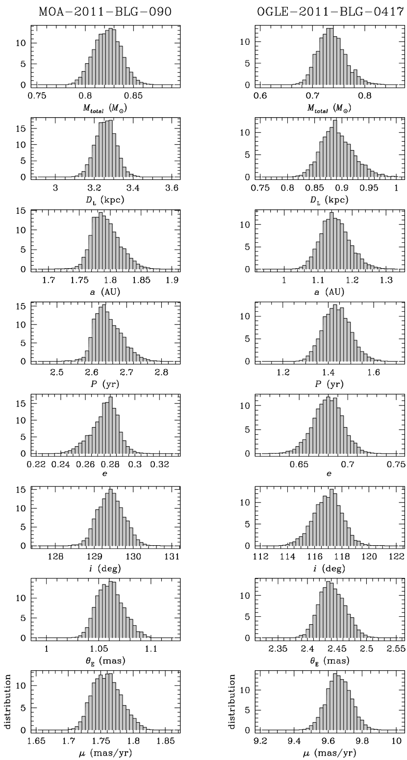
Figure 5.— Distributions of the physical and orbital parameters of the binary lens systems for MOA-2011-BLG-090 (left panels) and OGLE-2011-BLG-0417 (right panels).

6. DISCUSSION AND CONCLUSION

We reported detections and measurements of 2 binaries discovered from observations of microlensing events MOA-2011-BLG-090 and OGLE-2011-BLG-0417. The light curves of the events have common characteristics of long durations with caustic-crossing features, which enabled to determine the physical parameters of the lenses. It was found that both lens components of MOA-2011-BLG-090 and one component of OGLE-2011-BLG-0417 are M dwarfs. Therefore, the discovered microlensing binaries demonstrate the usefulness of gravitational lensing in detecting and characterizing binaries composed of low-mass stars. By considering full Keplerian binary motion, we also determined the orbital parameters of the binaries. For OGLE-2011-BLG-0417, the blended light comes very likely from the lens itself and thus it would be possible to check the orbital solution from follow-up radial-velocity observation.

Studies of M dwarfs are important not only because they are the most abundant stars in the Milky Way but also they form a link between solar-type stars and brown dwarfs; two mass regimes that might exhibit very different multiplicity characteristics. Precise knowledge of multiplicity characteristics and how they change in this transitional mass region provide constraints on low-mass star and brown dwarf formation (Goodwin et al., 2007; Burgasser et al., 2007). Despite the importance of M-dwarf binaries, only a few measurements of the binary fraction and distribution of low-mass stars have been made, e.g., Delfosse et al. (2004), and the samples are restricted to only binaries in the solar neighborhood. As a result, there are still large uncertainties about their basic physical properties as well as their formation environment. Considering the rapid improvement of lensing surveys both in equipment and strategy, it is expected that the number of microlensing binaries with measured physical parameters will increase rapidly. This will contribute to the complete view of stellar multiplicity across a wide range of binary parameters.

References

- Abt (1983) Abt, H. A. 1983, ARA&A, 21, 343
- Abt & Levy (1976) Abt, H. A., & Levy, S. G. 1976, ApJS, 30, 273
- Alard & Lupton (1998) Alard, C., & Lupton, R. H. 1998, ApJ, 503, 325
- Albrow et al. (2000) Albrow, M. D, et al. 2000, ApJ, 534, 894
- Albrow et al. (2009) Albrow, M. D, et al. 2009, MNRAS, 397, 2099
- An & Gould (2001) An, J., & Gould, A. 2001, ApJ, 563, L111
- Bessell & Brett (1988) Bessell, M. S., & Brett, J. M. 1988, PASP, 100, 1134
- Bond et al. (2001) Bond, I. A., et al. 2001, MNRAS, 327, 868
- Bramich (2008) Bramich, D. M. 2008, MNRAS, 386, L77
- Burgasser et al. (2007) Burgasser, A. J., et al. 2007, in Protostars and Planets V, ed. B. Reipurth, D. Jewitt, & K. Keil, 427
- Delfosse et al. (2004) Delfosse, X., et al. 2004, in Astronomical Society of the Pacific Conference Series, Vol. 318, Spectroscopically and Spatially Resolving the Components of the Close Binary Stars, ed. R. W. Hilditch
- Dong et al. (2006) Dong, Subo, et al., 2006, ApJ, 642, 842
- Dominik (1995) Dominik, M. 1995, A&AS, 109, 597
- Dominik (1998) Dominik, M. 1998, A&A, 329, 361
- Duquennoy & Mayor (1991) Duquennoy, A., & Mayor, M. 1991, A&A, 248, 485
- Goodwin et al. (2007) Goodwin, S. P., Kroupa, P., Goodman, A., & Burkert, A. 2007, Protostars and Planets, eds. V. B. Reipurth, D. Jewitt, & K. Keil (Tucson: Univ. of Arizona Press), 133
- Gaudi & Petters (2002) Gaudi, B. S., & Petters, A. O. 2002, ApJ, 580, 468
- Gaudi & Gould (1999) Gaudi, B. S., & Gould, A. 1999, ApJ, 513, 619
- Gould (1992) Gould, A. 1992, ApJ, 392, 442
- Gould (2000) Gould, A. 2000, ApJ, 542, 785
- Gould (2008) Gould, A. 2008, ApJ, 681, 1593
- Han & Gould (1995) Han, C., & Gould, A. 1995, ApJ, 447, 53
- Ioka et al. (1999) Ioka, K., Nishi, R., & Kan-Ya, Y. 1999, Prog. Theor. Phys., 102, 983
- Kayser et al. (1986) Kayser, R., Refsdal, S., & Stabell, R. 1986, A&A, 166, 36
- Kervella et al. (2004) Kervella, P., Thévenin, F., Di Folco, E., & Ségransan, D. 2004, A&A, 426, 297
- Mao & Paczyński (1991) Mao, S., & Paczyński, B. 1991, ApJ, 374, L37
- Pejcha & Heyrovský (2009) Pejcha, O., & Heyrovský, D. 2009, ApJ, 690, 1772
- Penny et al. (2011) Penny, M. T., Mao, S., & Kerins, E. 2011, MNRAS, 412, 607
- Refsdal (1966) Refsdal, S. 1966, MNRAS, 134, 315
- Schechter et al. (1993) Schechter, P. L., Mateo, M., & Saha, A. 1993, PASP, 105, 1342
- Schneider & Weiss (1986) Schneider, P., & Weiss, A. 1986, A&A, 164, 237
- Shin et al. (2011) Shin, I.-G., et al. 2011, ApJ, 735, 85
- Stanek & Garnavich (1998) Stanek, K. Z., & Garnavich, P. M. 1998, ApJ, 503, L131
- Skowron et al. (2011) Skowron, J., et al. 2011, ApJ, 738, 87
- Udalski (2003) Udalski, A. 2003, Acta Astron., 53, 291
- Wambsganss (1997) Wambsganss, J. 1997, MNRAS, 284, 172
- Yoo et al. (2004) Yoo, J., et al. 2004, ApJ, 603, 139