Parameterization dependence of $T$ matrix poles and eigenphases
from a fit to $\pi N$ elastic scattering data

Abstract

We compare fits to $\pi N$ elastic scattering data, based on a Chew-Mandelstam $K$-matrix formalism. Resonances, characterized by $T$-matrix poles, are compared in fits generated with and without explicit Chew-Mandelstam $K$-matrix poles. Diagonalization of the $S$ matrix yields the eigenphase representation. While the eigenphases can vary significantly for the different parameterizations, the locations of most $T$-matrix poles are relatively stable.

I Introduction

The excited states of the nucleon PDG have been studied in a wide array of reactions initiated mainly by pion and photon beams. Other approaches have involved an examination of the invariant mass distribution of products from, for example, nucleon-nucleon reactions morsch and $J/\Psi$ decays bes . Most states listed by the PDG PDG were identified from fits to $\pi N$ elastic scattering and reaction data. Photo-decay amplitudes were determined mostly through analyses of single-pion photoproduction data.

Recent measurements of cross section and polarization quantities, related to the photo- and electroproduction of states other than $\pi N$, have been analyzed separately and in multi-channel approaches. These studies have provided stronger evidence for states seen only weakly in $\pi N$ elastic scattering, and have suggested new states, coupling more strongly to other channels review .

Among the most extensive $\pi N$ scattering analyses KH80 ; CMB ; Arndt2006 , the parametrization of Ref.Arndt2006 based on the SAID interactive fitting and database codesSAID-website (the SAID-GW fit), utilizing the most recent data, has found the fewest number of $N$ and $\Delta$ resonances. In the fit of Ref. sm95 , a search for weaker structures was carried out. There, the existing solution was modified using a simple product S-matrix approach, to include the effect of an added Breit-Wigner resonance in each partial wave. Chi-squared was mapped for various combination of masses, widths and branching fraction. Two marginally significant candidates were found in the $S_{11}$ and $F_{15}$ partial waves, with pole positions: $1689-i96$ MeV (for $S_{11}$) and $1793-i94$ (for $F_{15}$). Of these, the $F_{15}$ has been reported in subsequent fits, while the $S_{11}$ has not.

^∗Deceased

^†Current address: Theory Division, Los Alamos National Laboratory, Los Alamos, NM 87545, USA

Here we have considered another approach. As detailed further below, existing GW-SAID fits to $\pi N$ elastic scattering data have utilized a fit form based on the Chew-Mandelstam (CM) $K$-matrix. This approach is capable of generating $T$-matrix poles without the assumption of explicit $K$-matrix poles. Previous fits have only included an explicit CM $K$-matrix pole for the $\Delta(1232)$. In the present study, an alternative parametrization with one explicit CM $K$-matrix pole in each partial wave is used to generate a fit independent of the usual CM parametrization form.

The motivation for this new fit is twofold. By changing the parameterization, we are able to gauge the stability of the amplitudes and resonance positions. We are also able to see if the addition of new explicit CM $K$-matrix poles translates into additional resonance signals.

Below, in Sec. II, we briefly review the CM $K$-matrix formalism used in this and previous fits. The eigenphase representation, and some numerical details, are reviewed in Sec. III. Results for the partial wave fits and resonance spectrum are compared in Sec. IV. Finally, in Sec. V, we consider the implication of this and future work.

II Chew-Mandelstam Formalism

The Chew-Mandelstam approach for the parametrization of multichannel hadronic $\pi N$ elastic scattering and reactions to other hadronic channels has been described in detail in Refs. sm95 ; Arndt85 ; Arndt03 ; Arndt2006 ; Paris:2010tz . The $\chi^{2}$-fits to data have been additionally constrained using the forward $C^{\pm}$ dispersion relations and fixed-t dispersion relations for the invariant $B$ amplitudes.

The standard CM parametrization can be expressed in terms of the on-shell Heitler partial wave $K$ matrix, $K$ as

$$K^{-1}(E)=\overline{K}^{\;-1}(E)-{\rm Re}C(E),$$ (1)

where $E$ is the (complex) scattering energy, $\overline{K}$ is the Chew-Mandelstam $K$ matrix and $C$ is a diagonal matrix, whose matrix elements are termed the Chew-Mandelstam functions Basdevant . The Heitler $K$ matrix is related to the partial wave transition amplitude matrix, $T$ as

$$T^{-1}(E)=K^{-1}(E)-i\rho(E).$$ (2)

Here, $\rho(E)=\delta(E-H_{0})$, where $H_{0}$ is the (model independent) relativistic free-particle Hamiltonian with physical (stable) particle masses. It determines the CM functions, $C(E)$ via the relation ${\rm Im}C(E)=\rho(E)$.

The standard form used in the GW fits is defined by the choice for the CM $K$-matrix elements

$$\overline{K}(E)=\sum_{n}c_{n}\overline{z}^{n}(E),$$ (3)

where $c_{n}$ are a set of constants and $\overline{z}$ is a linear function of the scattering energy, $E$. The integer, $n$ is typically between 2 and 5, and depends on the matrix element in question.

Note that $\overline{K}$ defines an entire function of the complex parameter $E$ for finite values. This form is used for all but the $P_{33}$ partial wave, which includes an explicit pole in $\overline{K}$. For partial waves other than the $P_{33}$, we see that the CM $K$ matrix, $\overline{K}$, is without poles (or other singularities). The Heitler $K$ matrix, $K$,

$$K={1\over{1-\overline{K}[{\rm ReC}]}}\overline{K}$$ (4)

has a pole whenever $\det[1-{\rm Re}C(E)\overline{K}(E)]=0$. The matrices $K$ and $\overline{K}$ are free of branch point singularities Zimmerman:1961aa ; Paris:2010tz .

The alternate form of the CM $K$ matrix is similar to the form used in the $P_{33}$ partial wave of the standard $\overline{K}$ parametrization, described above. This form is given by

$$\overline{K}_{ij}=\frac{\gamma_{i}\gamma_{j}}{E-E_{p}}+\beta(E)_{ij}.$$ (5)

Here, $\gamma_{i}(E)$ is a polynomial without a zero at the pole position, $E_{p}$, and the index labels the channel ($\pi N$, $\pi\Delta$, $\rho N$, and $\eta N$), $\beta(E)$ is an entire function of the complex energy, $E$.

III Eigenphase representation

The fit produces a unitary S-matrix of amplitudes for all contributing channels. While those channels not fitted to data are unlikely to give a quantitative representation of the reaction (for example $\pi N\to\pi\Delta$), they can be used to construct a set of eigenphases, which provide an interesting characterization of resonance behavior.

The unitarity of the $S$ matrix implies that its eigenvalues are phase factors. The matrix, $U$, of eigenvectors diagonalizes the $S$ matrix as

$$U^{\dagger}SU =\lambda,$$ (6)

where

$$\lambda =\left(\begin{matrix}\lambda_{1}&0&\cdots&0\\ 0&\lambda_{2}&\cdots&0\\ 0&0&\ddots&0\\ 0&0&\cdots&\lambda_{n}\end{matrix}\right).$$ (7)

Exploiting $|\lambda_{i}|=1$ we write

$$\lambda_{i} =e^{2i\phi_{i}}$$ (8)

with $\phi_{i}$ real.

Our objective is the numerical evaluation of the eigenphases given the $T$-matrix elements from various fits. This is straightforward at a given energy, using a standard routine to diagonalize the unitary $S$ matrix. The only complicating issue is correlating a given eigenphase, $\phi_{i}(E)$ with the appropriate eigenchannel when two (or more) eigenphases converge as the energy changes. In other words, once an eigenchannel $i$ is determined, we must track it for all energies. The no-crossing theoremWigner:1929nc is readily generalized to unitary matrices and shows that, in a given partial wave, the eigenphases may not be equal for any energy. This property is exhibited in the eigenphase plots discussed below.

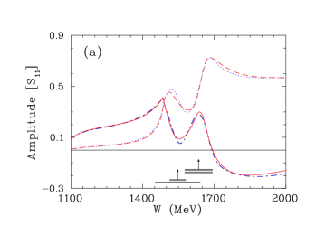
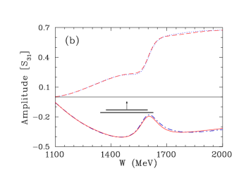
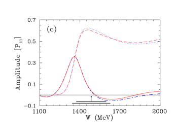
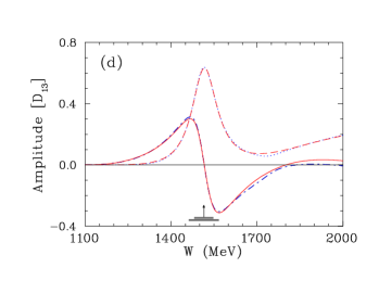
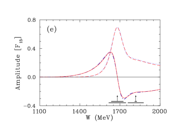
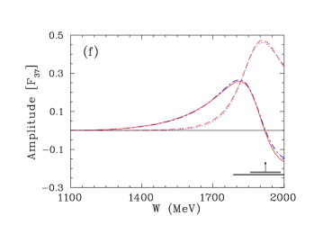
Figure 1: (Color online) Selected partial-wave amplitudes (L_2I,2J). Solid (dashed) curves give the real (imaginary) parts of amplitudes corresponding to the WI08 SAID-website solution. Dash-dotted (dotted) curves give the real (imaginary) parts of amplitudes corresponding to the XP08 solution. (a) $S_{11}$, (b) $S_{31}$, (c) $P_{11}$, (d) $D_{13}$, (e) $F_{15}$, and (f) $F_{37}$. All amplitudes are dimensionless. Vertical arrows indicate resonance $W_{R}$ values and horizontal bars show full $\Gamma$ and partial widths for $\Gamma_{\pi N}$.

Given the $T$ matrix at some energy, $T(E)$, we can form the $S(E)$ matrix. We diagonalize this matrix using a standard routine to obtain the eigenvalues $\{\lambda_{i}(E)\}_{i=1}^{n}$, where $n$ is the number of channels.

If the eigenvalues are nearly degenerate at some energy, it is difficult to distinguish which eigenvalue corresponds to a given eigenchannel, say $i$, since diagonalization of $S$ doesn’t preserve the eigenchannel ordering. The set of eigenvectors, however, must be orthogonal at any energy; and, for continuous partial wave amplitudes, the change of the eigenvector for a given eigenchannel is small for nearby energies.

The eigenchannels are maintained using the following method. The $S$ matrix is diagonalized at the initial energy, say $E_{1}=1150$ MeV. We obtain $n$ eigenphases (where $n$ is the number of channels included for the given partial wave), $\lambda_{1}(E_{1}),\ldots,\lambda_{n}(E_{1})$ and their corresponding eigenvectors $v_{1}(E_{1}),\ldots,v_{n}(E_{1})$. We wish to correlate the eigenvalues and eigenvectors with a given eigenchannel throughout the evaluation of the eigenvalues at higher energies, $E>E_{1}$.

Increasing the energy a small amount ($10-15$ MeV) to $E_{2}$, we again diagonalize the $S$ matrix and evaluate the $\lambda_{1}(E_{2}),\ldots,\lambda_{n}(E_{2})$ and eigenvectors $v_{1}(E_{2}),\ldots,v_{n}(E_{2})$.

In order to track the eigenchannel, we evaluate the matrix of overlaps:

$$O_{ij}(E_{1},E_{2}) =v_{i}(E_{1})^{\dagger}v_{j}(E_{2}).$$ (9)

As $E_{2}\to E_{1}$, we have

$$\lim_{E_{2}\to E_{1}}O_{ij}(E_{1},E_{2}) =\delta_{ij},$$ (10)

which is just the statement that the eigenvectors are orthonormal. For $E_{2}-E_{1}\simeq 10$ MeV, we identify the eigvenvalues according to the largest overlap in the set

$$\{|O_{ij}(E_{1},E_{2})|\}_{j=1}^{n}.$$ (11)

Suppose, for example, that we have three channels and at the energy $E_{1}$, we write the eigenvalues in the order:

$$\lambda_{1},\lambda_{2},\lambda_{3}.$$ (12)

And at energy $E_{2}$ for $i=1$, we find that

$$|O_{13}(E_{1},E_{2})|>|O_{11}(E_{1},E_{2})|>|O_{12}(E_{1},E_{2})|,$$ (13)

then for energy $E_{2}$ we order the eigenvalue $\lambda_{3}$ first; the ordering for the other eigenvalues is determined similarly.

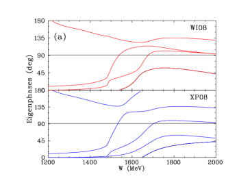
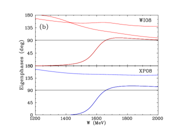
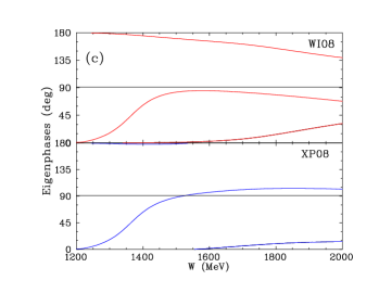
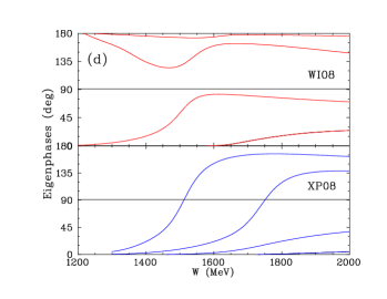
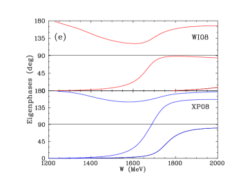
Figure 2: (Color online) Eigenphases. (a) $S_{11}$, (b) $S_{31}$, (c) $P_{11}$, (d) $D_{13}$, (e) $F_{15}$, and (f) $F_{37}$.

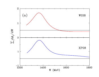
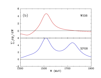
Figure 3: (Color online) Derivatives of eigenphases. (a) $P_{11}$ and (b) $D_{13}$.

IV Results

Table 1: Pole positions in complex energy plane of the $T$ matrix for the $\pi N\to\pi N$ reaction. The functional forms (see text) employed in the SAID fits are compared for selected partial waves. Each $T$ pole position is expressed in terms of its real and imaginary parts ($M_{R},-\Gamma_{R}/2$) in MeV. The second sheet pole is labeled by a $\dagger$.

$\ell_{JT}$	WI08			XP08
$S_{11}$	$(1499,49)$	$(1647,42)$	$(1666,260)$	$(1538,65)$	$(1675,58)$	$(1690,121)$
$S_{31}$	$(1594,68)$			$(1592,66)$
$P_{11}$	$(1358,80)$	$(1388,82)^{\dagger}$		$(1358,80)$	$(1387,80)^{\dagger}$	$(1646,290)$
$D_{13}$	$(1515,55)$			$(1513,53)$	$(1740,66)$	$(1716,370)$
$F_{15}$	$(1674,57)$	$(1779,138)$		$(1672,70)$	$(1734,61)$
$F_{37}$	$(1883,115)$			$(1874,119)$

The fits with (XP08) and without (WI08) explicit CM $K$-matrix poles, in waves other than $(L_{2I,2J})$ $P_{33}$, are compared in Fig. 1. Differences in the partial waves are slight, and the fit quality is comparable over the resonance region, each fit using a similar number of parameters. This feature of the $\pi N$ elastic scattering analysis seems quite stable.

In Fig. 2, we have calculated the eigenphases corresponding to the full S-matrix. Only the $\pi N\to\pi N$ and $\pi N\to\eta N$ channels have been constrained by data. The behavior of these phases does, however, provide an interesting perspective on the emergence of resonance structures in the fits.

In the $S_{11}$ partial wave, both fits have two eigenphases crossing 90 degrees, at 1535 and 1670 MeV for WI08, and at 1530 and 1700 MeV for XP08. If one computes the usual Heitler $K$ matrix, as was done in Ref. WAP , $K$-matrix poles are found at these energies (since the unitary transformation, $U$ [Eq.(6)] diagonalizes $K$ simultaneously with $S$ and $K_{ii}=\tan\phi_{i}$). In the $S_{31}$ partial wave, a 2- and 3-channel fit are compared, yielding identical crossing energies, again corresponding to a $K$-matrix pole (at 1655 MeV). Note that in the WI08 plot, two eigenphase nearly touch, but do not cross.

In the $P_{11}$ plot, only one of the solutions has a 90 degree crossing leading to a $K$-matrix pole. Note, however, that the energy dependence of the eigenphase crossing, and nearly crossing 90 degrees, is very similar. This feature determines another measure of resonance behavior, to be discussed below.

The $D_{13}$ eigenphases are quite different in the two fits. In the WI08 fit, there are no 90 degree crossings, while in XP08, we see two crossings. This hints at a different resonance structure, though the $\pi N$ $T$ matrices are nearly identical.

In the $F_{15}$ and $F_{37}$ eigenphase plots, the XP08 solution has a single crossing, whereas the WI08 solution does not. Here also, a comparison of the eigenphases which cross, or come close to crossing, 90 degrees have a similar energy dependence.

As has been noted previouslyCeci:2008kt , resonances may be associated with a single eigenphase crossing 90 degrees, and this will result in a $K$-matrix pole. However, a more robust measure (if a set of amplitudes is available) is given by the time-delay matrix res , which is proportional to the sum of energy derivatives of all eigenphases. Other factors, such as threshold openings can also produce rapid energy dependence. Certainly the correct method of resonance identification requires the location of poles in the complex energy plane on unphysical sheets close to the physical region, which we demonstate below. Our employment of the eigenphase approach illustrates the fact that resonance structure may vary with the appearance of resonances in different parametrizations without significantly altering the shape of the $\pi N$ elastic amplitude. It is usually the case, however, that such resonances are deep in the complex plane having large widths.

In Fig. 3, for illustration, we plot the sum of eigenphase energy derivatives for the $P_{11}$ and $D_{13}$. The peaks for $P_{11}$ are nearly identical and occur at about 1350 MeV, which (we will see) corresponds with the real part of the pole position. For the $D_{13}$, peaks corresponding the the 4-star state, near 1500 MeV, are closely aligned. The second peak has almost no evidence in the $\pi N$ elastic amplitude. However, a large contribution to the (unfitted and therefore unconstrained) $\pi\Delta$ or $\rho N$ channels would result in the second peak.

In Table 1, we compare the pole positions associated with resonance behavior in the plotted amplitudes. The third $S_{11}$ pole in XP08 closely resembles the structure found in Ref. sm95 , at $(1689,96)$ MeV, by scanning all partial waves with an added Breit-Wigner contribution. The very broad $(1646,290)$ MeV $P_{11}$ state is similarly close to one found in the SM90 fit sm90 , at $(1636,272)$ MeV. Two extra poles were found in the $D_{13}$ partial wave for the XP08 solution compared to WI08. We do not intend to report the $(1716,370)$ MeV pole as a resonance but merely mention it here in connection with the present sensitivity study. Interestingly, the pole at $(1740,66)$ MeV has its effect masked by a zero intervening between the pole and real energy axis and therefore makes little impact in the physical region.

V Conclusion

We have reported a study of the parameterization dependence of our $\pi N$ elastic amplitudes and resonance spectrum, using a very different form for the CM $K$ matrix, with explicit poles in each partial wave. The partial-wave amplitudes were found to be very stable with the change.

The eigenphase representation was introduced, mainly as a novel approach to resonance identification, and because it provides a more concrete example of properties discussed in older works. This discussion also provides a continuation of the study started in Ref. WAP .

The more formally correct extraction of pole positions has revealed structures mainly found in earlier fits to the $\pi N$ elastic scattering data. As the partial wave amplitudes have not changed significantly, the effects of new resonances must be minimized through large widths, intervening zeros, or small coupling to the $\pi N$ channel.

In the SM90 fit, a study of the resonance spectrum was tried where, in addition to experimental data, the amplitudes from the KH KH80 and CMB CMB analyses were added as soft constraints. A possible extension to the present work would be a re-examination of the resonance spectrum from a fit, with explicit CM $K$-matrix poles, constrained to more closely follow either the KH and CMB analyses, or a multi-channel analysis.

- (1) K. Nakamura, et al. (Particle Data Group), J. Phys. G 37, 075201 (2010).
- (2) P. Morsch, Int. J. Mod. Phys. A 20, 1699 (2005).
- (3) M. Ablikim et al., Phys. Rev. Lett. 97, 06201 (2006).
- (4) For a review, see E. Klempt and J. M. Richard, Rev. Mod. Phys. 82, 1095 (2010).
- (5) G. Höhler, Pion-Nucleon Scattering, ed. H. Schopper, Vol. I/9b2 (Landolt-Börnstein, Springer Verlag, 1983).
- (6) R. E. Cutkosky et al., IV International Conference on Baryon Resonances (Baryon 1980), Toronto, ed. N. Isgur, p. 19.
- (7) R. A. Arndt et al., Phys. Rev. C 74, 045205 (2006).
- (8) A selection of fits and the full database are available at: http://gwdac.phys.gwu.edu.
- (9) R. A. Arndt, I. I. Strakovsky, R. L. Workman, and M. M. Pavan, Phys. Rev. C 52, 2120 (1995).
- (10) R. A. Arndt, J. M. Ford, and L. D. Roper, Phys. Rev. D 32, 1085 (1985).
- (11) R. A. Arndt, W. J. Briscoe, I. I. Strakovsky, R. L. Workman, and M. M. Pavan, Phys. Rev. C 69, 035213 (2004).
- (12) M. W. Paris and R. L. Workman, Phys. Rev. C 82, 035202 (2010).
- (13) J.-L. Basdevant and E. L. Berger, Phys. Rev. D 19, 239 (1979).
- (14) W. Zimmerman, Nuovo Cim. 21, 249 (1961).
- (15) E. P. Wigner and J. von Neumann, Z. Phys. 30, 467 (1929).
- (16) R. L. Workman, R. A. Arndt, and M. W. Paris, Phys. Rev. C 79, 038201 (2009).
- (17) S. Ceci et al., Phys. Lett. B 659, 228 (2008).
- (18) R. H. Dalitz and R. G. Moorhouse, Proc. Roy. Soc. Lond. 318, 279 (1970); F. T. Smith, Phys. Rev. 118, 349 (1960).
- (19) R. A. Arndt, Z. Li, L. D. Roper, R. L. Workman, and J. M. Ford, Phys. Rev. D 43, 2131 (1991).