The Aharonov–Bohm effect for massless Dirac fermions
and the spectral flow of Dirac type operators
with classical boundary conditions

Abstract

We compute, in topological terms, the spectral flow of an arbitrary family of self-adjoint Dirac type operators with classical (local) boundary conditions on a compact Riemannian manifold with boundary under the assumption that the initial and terminal operators of the family are conjugate by a bundle automorphism. This result is used to study conditions for the existence of nonzero spectral flow of a family of self-adjoint Dirac type operators with local boundary conditions in a two-dimensional domain with nontrivial topology. Possible physical realizations of nonzero spectral flow are discussed.

Keywords: Aharonov–Bohm effect, massless Dirac fermions, graphene, topological insulators, self-adjoint Dirac operator, spectral flow, Atiyah–Singer index theorem, Atiyah–Bott index theorem, index locality principle.

1 Introduction

Not to mention high-energy physics and quantum field theory, the ideas of modern geometry and topology become increasingly important in condensed matter physics [1, 2, 3, 4, 5, 6, 7, 8, 9]. In particular, the Atiyah–Singer index theorem [10] explains a topological protection of zero-energy Landau level and related peculiarities of the quantum Hall effect in graphene [6, 7]. Topologically protected zero modes play an essential role in the motion of vortices in superfluid helium-3 [5, 11]. The quantum Hall effect [2, 3] and topological insulators [8, 9] are examples of the states of matter with topological order parameter.

The Aharonov–Bohm effect (ABE) [12, 13] has actually initiated this development. A magnetic flux localized in a region completely unavailable for a quantum particle (e.g., surrounded by infinitely high potential barrier) nevertheless affects its motion, modifying the geometry of quantum space. A periodic dependence of electron energy levels in a ring as a function of the magnetic flux through the ring resulting in appearance of a persistent current (see Ref. [14] and references therein) is a bright manifestation of ABE. When the change of the magnetic flow is equal to an integer number of the flux quanta, the energetic spectrum should return to its initial state. Until recently, ABE was studied mainly for usual nonrelativistic electrons described by the Schrödinger equation. After discovery of graphene, the ABE for ultrarelativistic electrons described by Dirac equation with zero mass has attracted attention [15, 16, 17]. From the mathematical point of view, this is a much richer case. The Dirac operator is not semibounded and hence its spectral flow [18] can be nonzero. It is worth noting that the nonzero spectral flow of the Dirac operator has been discussed already in a context of condensed matter physics. It results in additional forces (“Kopnin forces”) acting on vortices in superfluid helium-3 [5, 11]. Coming back to ABE, it means that the coincidence of the whole energy spectra at the change of the magnetic flux at integer number of the flux quanta does not necessarily mean the periodicity of individual eigenenergies (like the shift $m\rightarrow m+1$ transforms $Z$ to itself). Nonzero spectral flow corresponds to a physical situation when an adiabatically slowly varying magnetic field leads to a production of electron–hole (or, in general, particle–antiparticle) pairs from the vacuum: “positron” levels cross zero-energy level transforming into electron ones. The vacuum reconstruction effects were discussed in physics of superfluid helium-3 [5] and in physics of graphene [7] but without any relation with ABE. Here we study conditions of existence of nonzero spectral flow of a family of Dirac-like self-adjoint operators with local boundary conditions in a domain with nontrivial topology.

In a bounded domain $X\subset\mathbb{R}^{2}$ with smooth boundary $\partial X$ (see Fig. 1), consider the boundary value problem

$$\biggl{(}\begin{matrix}0&-i\frac{\partial}{\partial x}-\frac{\partial}{\partial y}\\ -i\frac{\partial}{\partial x}+\frac{\partial}{\partial y}&0\\ \end{matrix}\biggr{)}\begin{pmatrix}u_{1}\\ u_{2}\\ \end{pmatrix}u=\begin{pmatrix}f_{1}\\ f_{2}\\ \end{pmatrix}\quad\text{in $X$},\quad(n_{y}-in_{x})u_{1}=Bu_{2}\quad\text{on $\partial X$,}$$ (1)

where $n_{x}$ and $n_{y}$ are the inward normal components and $B$ is a nonvanishing real-valued function on the boundary. (Berry and Mondragon [19] were the first to consider boundary conditions of this kind.)

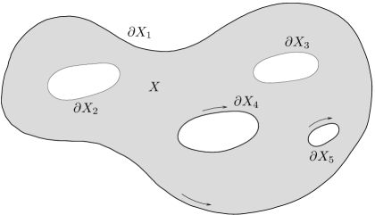
Figure 1: Example of a domain $X$ with $m=5$ boundary components. The bold lines show the boundary components $\partial^{+}\!X=\partial X_{1}\cup\partial X_{4}\cup\partial X_{5}$ on which $B>0$ in the boundary condition in (1). (It is only these components that contribute to the spectral flow according to formula (3).) The arrows show the positive sense of going around the contour when computing the winding number of the gauge transformation $\mu$ along the corresponding boundary component.

The operator $D_{0}$ corresponding to this problem is self-adjoint and Fredholm on $L^{2}(X,\mathbb{C}^{2})$. Next, let $\mu$ be a smooth function on $X$ with $\lvert\mu\rvert=1$. The “gauge transformation” $D_{0}\to\mu D_{0}\mu^{-1}$ takes $D_{0}$ to the operator $D_{1}=D_{0}+Q_{1}$ (where $Q_{1}$ is a self-adjoint matrix function) with the same boundary conditions. In physicists’ language, the gradient of the phase $\mu$ is an abelian ($U(1)$) gauge field, i.e., an electromagnetic vector potential. We consider a two-dimensional domain with $m-1$ holes pierced by magnetic flux tubes. The case in which all magnetic fluxes through the holes are integer multiples of the magnetic flux quantum corresponds to $\mu=1$. Let us join $Q_{1}$ with $Q_{0}=0$ by a continuous family $Q_{t}$, $t\in[0,1]$, of self-adjoint matrix functions. The spectral flow $\operatorname{sf}\{D_{t}\}$ of the family

$$D_{t}=D_{0}+Q_{t},$$ (2)

i.e., the number of eigenvalues of $D_{t}$ that changed their sign from minus to plus as the parameter $t$ varies from $0$ to $1$ minus the number of eigenvalues that changed their sign from plus to minus, does not change under continuous deformations of the family provided that $D_{0}$ and $D_{1}$ remain isospectral in the course of deformation. As far as the authors know, the problem of finding this spectral flow (also for families of Dirac operators of more general form) was posed for the first time and partially solved in [20], where the spectral flow was computed up to an integer factor $c_{m}$ depending on the number $m$ of boundary components. Further, it was shown in [20] that $c_{2}=1$, and it was conjectured that $c_{m}=1$ for all $m$. In the present paper, we establish a general result (see Theorem 2 below), which, in particular, proves this conjecture to be true. Thus, Theorem 1 in [20] acquires the following form:

Theorem 1.

The spectral flow of the family (2) is given by the formula

$$\operatorname{sf}{D_{t}}=\operatornamewithlimits{wind}_{\partial\mathstrut^{+}\!X}\mu,$$ (3)

where $\partial\mathstrut^{+}\!X$ is the part of $\partial X$ where $B>0$ and

$$\operatornamewithlimits{wind}_{\partial\mathstrut^{+}\!X}\mu=\frac{1}{2\pi i}\oint_{\partial\mathstrut^{+}\!X}\frac{d\mu}{\mu}$$

is the winding number of the restriction of the function $\mu$ to $\partial\mathstrut^{+}\!X$. (The set $\partial\mathstrut^{+}\!X$ is a union of finitely many circles; when defining the winding number, the positive sense of any of these circles is the one for which the domain $X$ remains to the left when moving along the circle.)

This theorem shows that the coefficients $c_{m}$ that remained unfound in [20, Theorem 1] are equal to unity for all $m$. The same is true for [20, Theorems 2 and 3]; all unknown coefficients $c_{m}$ occurring there are equal to unity.

Theorem 1 follows from a general result established in the present paper. We give a computation in topological terms of the spectral flow of an arbitrary family $\{D_{t}\}$, $t\in[0,1]$, of self-adjoint Dirac type operators with local boundary conditions on a compact Riemannian manifold $X$ with boundary $\partial X$ under the assumption that $D_{1}=UD_{0}U^{-1}$, where $U$ is some automorphism of the bundle in which the operators $D_{t}$ act. (In contrast with [20], we assume neither that the principal part of $D_{t}$ is independent of $t$ nor even that the principal parts of $D_{0}$ and $D_{1}$ coincide.) Namely, we prove (see Theorem 2 below) that

$$\operatorname{sf}\{D_{t}\}=\operatorname{ind}\biggl{(}\frac{\partial}{\partial t}+D\biggr{)},$$ (4)

where the right-hand side is the index of an elliptic operator with boundary conditions on the manifold $X\times S^{1}$ with boundary, $t$ being the coordinate on the circle $S^{1}$ and the operator $D$ being obtained from the family $\{D_{t}\}$ by clutching the operators $D_{0}$ and $D_{1}$ with the use of the automorphism $U$. (Recall that formula (4) for families of self-adjoint elliptic operators on a closed manifold $X$ was established in [18].) The right-hand side of (4) can be computed by the Atiyah–Bott formula [21] (see also [22, Sec. 20.3]). Note, however, that we do not rely on the Atiyah–Bott formula in the proof of Theorem 1; relation (4) between the spectral flow and the index permits one to use the localization method (see [23, 24, 25]) and cut the domain into parts, thus reducing the problem to the case of a domain with one hole ($m=2$), for which a straightforward computation was carried out in [20]. Note also that the localization method proves to be an important technical tool when proving relation (4) itself. The proof is in many aspects similar to that in [26, Proposition 5.6] of the spectral flow formula for families of differential operators Agranovich–Vishik elliptic with parameter on a closed compact manifold but contains a number of new important lines of argument related to the presence of boundary conditions.

2 Spectral Flow

Recall the definition of spectral flow in the form presented in [26] (cf. [27]). Let $\{B_{t}\}$, $t\in[0,1]$, be a family, continuous in the sense of uniform resolvent convergence, of unbounded self-adjoint operators with purely discrete spectrum on a Hilbert space $\mathcal{H}$. Then there exists a partition $0=t_{0}<t_{1}<t_{2}<\dotsm<t_{n+1}=1$ of the interval $[0,1]$ and real numbers $\gamma_{1},\dotsc,\gamma_{n+1}$ such that $\gamma_{j}$ does not lie in the spectrum $\operatorname{Spec}(B_{t})$ of the operator $B_{t}$ for $t\in[t_{j-1},t_{j}]$, $\gamma_{1}=\gamma_{n+1}\leq 0$, and if $\gamma_{1}<0$, then the half-open interval $[\gamma_{1},0)$ does not contain any points of spectrum of $B_{0}$ and $B_{1}$.

Definition 1 (see [26], Definition A.18).

The spectral flow of the family $\{B_{t}\}$, $t\in[0,1]$, is the number

$$\operatorname{sf}\{B_{t}\}=\sum_{j=1}^{n}m_{j}\operatorname{sign}(\gamma_{j}-\gamma_{j+1}),$$ (5)

where $m_{j}$ is the number of eigenvalues (counting multiplicities) of the operator $B_{t_{j}}$ on the interval between $\gamma_{j}$ and $\gamma_{j+1}$.

This definition is illustrated in Fig. 2, which, in particular, clarifies why this definition is consistent with the notion of spectral flow as the number of eigenvalues passing through zero (with direction taken into account).

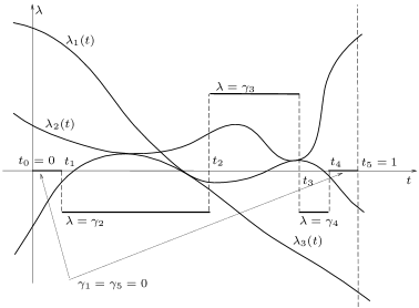
Figure 2: Definition of spectral flow. There are three eigenvalues $\lambda_{j}(t)$, $j=1,2,3$, contributing to the spectral flow. Both the computation according to the definition and counting the number of zero crossings (with regard to direction) give the value $-1$ for the spectral flow.

3 Main Results

Let $E$ be an even-dimensional Hermitian vector bundle over a compact Riemannian manifold $X$ with boundary, and let

$$A\colon C^{\infty}(X,E)\longrightarrow C^{\infty}(X,E)$$ (6)

be a formally self-adjoint Dirac type operator. Next, let a subbundle $L\subset E_{Y}$ of dimension $\dim L=\frac{1}{2}\dim E$ be given in the restriction $E_{Y}$ of the bundle $E$ to the boundary $Y=\partial X$ of the manifold $X$ such that

$$\bigl{(}\sigma_{A}(x,\mathbf{n}(x))L_{x}\bigr{)}\perp L_{x}\qquad\forall x\in Y,$$ (7)

where $L_{x}$ is the fiber of $L$ at $x$ and $\mathbf{n}(x)$ is the unit inward conormal vector on the boundary. Consider the operator (6) on the set of sections $u\in C^{\infty}(X,E)$ satisfying the homogeneous boundary condition

$$\pi_{L}(u|_{Y})=0,\quad\text{where }\pi_{L}\colon E_{Y}\longrightarrow E_{Y}/L\quad\text{is the natural projection.}$$ (8)

(In other words, $u(x)\in L_{x}$ for $x\in Y$.) In particular, the boundary condition in (1) is of this form. It is well known (see [29] and [28, Chaps. 18 and 19]) that the boundary condition (8) is elliptic, the operator (6) with domain given by this condition is essentially self-adjoint on $L^{2}(X,E)$, and its closure $A_{L}$ is an unbounded Fredholm self-adjoint operator on $L^{2}(X,E)$ with discrete spectrum and with domain consisting of sections $u$ belonging to the Sobolev space $H^{1}(X,E)$ and satisfying condition (8) (in which $u|_{Y}$ is treated as the element of $H^{1/2}(Y,E_{Y})$ obtained from $u$ by restriction to $Y$ by virtue of the trace theorem and $\pi_{L}$ is treated as a mapping $\pi_{L}\colon H^{1/2}(Y,E_{Y})\longrightarrow H^{1/2}(Y,E_{Y}/L)$).

Now assume that both the Dirac type operator $A$ (6) and the subbundle $L$ continuously depend on a parameter $t\in[0,1]$ (namely, the coefficients of $A$ and $\pi_{L}$ depend on $t$ continuously together with all of their derivatives); i.e., $A=A(t)$ and $L=L(t)$. Moreover, assume that condition (7) holds for each $t$. Then, by Theorem 7.16 in [30], the operator $A(t)_{L(t)}$ continuously depends on $t$ in the topology of uniform resolvent convergence, and Definition 1 specifies the spectral flow $\operatorname{sf}\{A(t)_{L(t)}\}$ of the family $\{A(t)_{L(t)}\}$, $t\in[0,1]$.

Next, let an automorphism $U\colon E\to E$ of the bundle $E$ be given such that

$$A(1)=UA(0)U^{-1},\qquad U(L(0))=L(1).$$ (9)

Then $UA(0)_{L(0)}U^{-1}=A(1)_{L(1)}$; i.e., the operators $A(0)_{L(0)}$ and $A(1)_{L(1)}$ are similar and hence isospectral, so that the spectral flow of the family $\{A(t)_{L(t)}\}$ is a homotopy invariant (in the class of families satisfying a condition of the form (9)). Thus, it is natural to pose the problem of computing it in topological terms.

To do this, we introduce an auxiliary elliptic boundary value problem on the Cartesian product $X\times S^{1}$ of the manifold $X$ by the circle $S^{1}$ (see Fig. 3). Namely, let us define a bundle $\mathcal{E}$ over $X\times S^{1}$ as follows. Take the pullback of $E$ to the product $X\times[0,1]$ via the natural projection $\pi\colon X\times[0,1]\to X$ and then use the automorphism $U\colon(\pi^{*}E)_{X\times\{0\}}\longrightarrow(\pi^{*}E)_{X\times\{1\}}$ as the clutching automorphism. By conditions (9), the family $\{A(t)\}$ specifies a well-defined differential operator on the space of sections of the bundle $\mathcal{E}$, while the family of subbundles $L(t)$ defines a subbundle $\mathcal{L}\subset\mathcal{E}_{Y\times S^{1}}$ in the restriction of $\mathcal{E}$ to the boundary $Y\times S^{1}$ of the manifold $X\times S^{1}$.

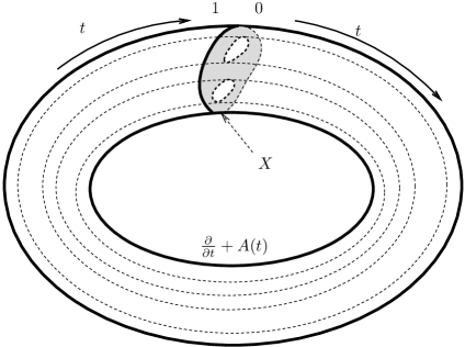
Figure 3: The manifold $X\times S_{1}$ obtained by gluing together the faces $t=0$ and $t=1$ of the product $X\times[0,1]$, and the operator $\frac{\partial}{\partial t}+A(t)$.

Proposition 1.

The operator

$$\frac{\partial}{\partial t}+A(t)\;\colon C^{\infty}(X\times S^{1},\mathcal{E})\longrightarrow C^{\infty}(X\times S^{1},\mathcal{E})$$ (10)

is elliptic, and the boundary conditions

$$\pi_{\mathcal{L}}(u|_{Y\times S^{1}})=0,\quad\text{where }\pi_{\mathcal{L}}\colon\mathcal{E}_{Y\times S^{1}}\longrightarrow\mathcal{E}_{Y\times S^{1}}/\mathcal{L}\quad\text{is the natural projection,}$$ (11)

defined by the subbundle $\mathcal{L}$, are elliptic for the operator (10). The closure $\bigl{(}\frac{\partial}{\partial t}+A(t)\bigr{)}_{\mathcal{L}}$ of the operator (10) from the domain specified by conditions (11) is an unbounded Fredholm operator on $L^{2}(X\times S^{1},\mathcal{E})$ with domain $\mathfrak{D}_{\mathcal{L}}$ consisting of the sections $u\in H^{1}(X\times S^{1},\mathcal{E})$ satisfying condition (11).

Now we are in a position to state the main theorem of the present paper.

Theorem 2.

One has

$$\operatorname{sf}\{A(t)_{L(t)}\}=\operatorname{ind}\biggl{(}\frac{\partial}{\partial t}+A(t)\biggr{)}_{\mathcal{L}}.$$ (12)

The right-hand side of (12) is the analytic index of the operator $\bigl{(}\frac{\partial}{\partial t}+A(t)\bigr{)}_{\mathcal{L}}$, i.e., the difference of dimensions of its kernel and cokernel, which can be expressed in topological terms by the Atiyah–Bott formula [21] (see also [22, Sec. 20.3]).

4 Proof of the Main Assertions

Proof of Proposition 1.

Consider the operator

$$\mathfrak{A}=\begin{pmatrix}0&\frac{\partial}{\partial t}+A(t)\\ -\frac{\partial}{\partial t}+A(t)&0\\ \end{pmatrix}\colon C^{\infty}(X\times S^{1},\mathcal{E}\oplus\mathcal{E})\longrightarrow C^{\infty}(X\times S^{1},\mathcal{E}\oplus\mathcal{E}).$$ (13)

This is a total formally self-adjoint Dirac type operator on $X\times S^{1}$ with symbol

$$\sigma_{\mathfrak{A}}(x,t,\xi,\xi_{0})=\begin{pmatrix}0&i\xi_{0}I+\sigma_{A(t)}(x,\xi)\\ -i\xi_{0}I+\sigma_{A(t)}(x,\xi)&0\\ \end{pmatrix},$$ (14)

where $\xi_{0}$ is the momentum variable conjugate to $t\in S^{1}$, and the operator $\frac{\partial}{\partial t}+A(t)$ is its chiral part. The subbundle $\mathfrak{L}=\mathcal{L}\oplus\mathcal{L}\subset(\mathcal{E}\oplus\mathcal{E})_{Y\times S^{1}}$ satisfies a condition of the form (7) with respect to $\sigma_{\mathfrak{A}}$ and hence specifies self-adjoint elliptic boundary conditions for $\mathfrak{A}$. Indeed, the conormal vector to the boundary of $X\times S^{1}$ at an arbitrary point $(x,t)\in Y\times S^{1}$ has the form $\mathfrak{n}(x,t)=(0,\mathbf{n}(x))$, where $\mathbf{n}(x)$ is the conormal vector to the boundary of $X$ itself and $\mathcal{L}_{(x,t)}=L(t)_{x}$; hence, for any

$$v={}^{t}(v_{1},v_{2})\in\mathfrak{L}_{(x,t)},\quad w={}^{t}(w_{1},w_{2})\in\mathfrak{L}_{(x,t)},\qquad\text{i.e., $v_{1},v_{2},w_{1},w_{2}\in L(t)_{x}$},$$

we have

$$(v,\sigma_{\mathfrak{A}}(x,t,\mathfrak{n}(x,t))w)=(v_{1},\sigma_{A(t)}(x,\mathbf{n}(x))w_{2})+(v_{2},\sigma_{A(t)}(x,\mathbf{n}(x))w_{1})=0,$$

because condition (7) is satisfied for $A(t)$ and the bundle $L(t)$. This, again by virtue of the results in [29] and [28, Chaps. 18 and 19], implies the claim of Proposition 1 first for the operator $\mathfrak{A}$ and then, as a consequence, for its chiral part $\frac{\partial}{\partial t}+A(t)$. ∎

Proof of Theorem 2.

a. Without loss of generality, we assume that $0\notin\operatorname{Spec}(A(0)_{L(0)})$. (Otherwise, one can replace the operator $A(t)$ by $A(t)+\varepsilon$ with small real $\varepsilon$, which changes neither the left- nor the right-hand side of (12).)

b. Also without loss of generality, we assume throughout the following that the subbundle $L(t)$ is independent of the parameter $t$, $L(t)=L(0)\equiv L$, $t\in[0,1]$. Indeed, let $V(t)\colon E_{Y}\to E_{Y}$ be a family of unitary automorphisms of $E_{Y}$ such that $V(0)=I$ and $L(t)=V(t)L$, $t\in[0,1]$. (One can readily construct such a family by solving the Cauchy problem $\dot{V}=[P,\dot{P}]V$, $V(0)=I$, where $P=P(t)$ is the projection onto $L(t)$ in $E_{Y}$.) This family can be continued (by a homotopy to the identity mapping along the variable normal to the boundary) to a family of unitary automorphisms $W(t)\colon E\to E$ such that $W(t)\big{|}_{Y}=V(t)$. Set

$$\widetilde{A}(t)=W^{-1}(t)A(t)W(t);$$

then, obviously,

$$W^{-1}(1)U\widetilde{A}(0)(W^{-1}(1)U)^{-1}=W^{-1}(1)U\widetilde{A}(0)U^{-1}W(1)=W^{-1}(1)A(1)W(1)=\widetilde{A}(1),$$

$$W^{-1}(1)UL\equiv W^{-1}(1)UL(0)=W^{-1}(1)L(1)=L(0)\equiv L;$$

i.e., conditions of the form (9) are satisfied for the family $\{\widetilde{A}(t)\}$ and the constant family of subspaces $\widetilde{L}(t)=L$ if one takes the automorphism $\widetilde{U}=W^{-1}(1)U$. Furthermore,

$$\operatorname{sf}\{A(t)_{L(t)}\}=\operatorname{sf}\{\widetilde{A}(t)_{L}\},$$ (15)

because the operators $A(t)$ and $\widetilde{A}(t)$ are similar. Next, the family $W(t)$ generates a bundle isomorphism $\mathcal{W}\colon\widetilde{\mathcal{E}}\to\mathcal{E}$, where the bundle $\widetilde{\mathcal{E}}$ over $X\times S^{1}$, by analogy with $\mathcal{E}$, is obtained from the pullback of $E$ to $X\times[0,1]$ by clutching with automorphism $\widetilde{U}$. The operator

$$\mathcal{W}^{-1}\biggl{(}\frac{\partial}{\partial t}+A(t)\biggr{)}_{\mathcal{L}}\mathcal{W}=\biggl{(}\frac{\partial}{\partial t}+\widetilde{A}(t)-W^{-1}(t)\frac{\partial W}{\partial t}(t)\biggr{)}_{\widetilde{\mathcal{L}}}$$ (16)

has the same index as $\bigl{(}\frac{\partial}{\partial t}+A(t)\bigr{)}_{\mathcal{L}}$ and acts on the space of sections of $\widetilde{\mathcal{E}}$ satisfying the boundary condition associated with the subbundle $\widetilde{\mathcal{L}}=\mathcal{W}^{-1}\big{|}_{Y\times S^{1}}\mathcal{L}$, for which $\widetilde{\mathcal{L}}_{t}=V(t)^{-1}L(t)=L$ for all $t\in S^{1}$. Finally, the homotopy

$$\biggl{(}\frac{\partial}{\partial t}+\widetilde{A}(t)-\lambda W^{-1}(t)\frac{\partial W}{\partial t}(t)\biggr{)}_{\widetilde{\mathcal{L}}},\qquad\lambda\in[0,1],$$ (17)

in the class of Fredholm operators reduces the operator (16) for $\lambda=0$ to $\bigl{(}\frac{\partial}{\partial t}+\widetilde{A}(t)\bigr{)}_{\widetilde{\mathcal{L}}}$, so that

$$\operatorname{ind}\biggl{(}\frac{\partial}{\partial t}+A(t)\biggr{)}_{\mathcal{L}}=\operatorname{ind}\biggl{(}\frac{\partial}{\partial t}+\widetilde{A}(t)\biggr{)}_{\widetilde{\mathcal{L}}},$$

which, together with (15), completes reduction to the case of a bundle $L(t)=L$ independent of $t$. We omit the tilde over letters in what follows.

c. In the proof, we need a family of operators on the infinite cylinder $X\times\mathbb{R}$. Let us describe it. The pullbacks of the bundle $E$ from $X$ to $X\times\mathbb{R}$ and the bundle $L$ from $Y$ to $Y\times\mathbb{R}$ will be denoted by the same letters $E$ and $L$, respectively; this shall not lead to confusion. The coordinate on the line $\mathbb{R}$ will be denoted by $t$. For $\alpha,\beta\in\mathbb{R}$, we introduce the weighted spaces $L^{2}_{\alpha\beta}(X\times\mathbb{R},E)$ and $H^{1}_{\alpha\beta}(X\times\mathbb{R},E)$ of sections $u$ of $E$ with finite norm

$$\left\|u\right\|_{0,\alpha\beta} =\biggl{\{}\int_{-\infty}^{0}\left\|{u(t)}\right\|_{L^{2}(X,E)}^{2}e^{2\alpha t}\,dt+\int_{0}^{\infty}\left\|{u(t)}\right\|_{L^{2}(X,E)}^{2}e^{2\beta t}\,dt\biggr{\}}^{1/2}\qquad\text{and}$$

$$\left\|{u}\right\|_{1,\alpha\beta} =\biggl{\{}\int_{-\infty}^{0}\biggl{(}\left\|{\vphantom{\Big{|}}\smash{\frac{\partial u(t)}{\partial t}}}\right\|_{L^{2}(X,E)}^{2}+\left\|{u(t)}\right\|_{H^{1}(X,E)}^{2}\biggr{)}e^{2\alpha t}\,dt$$

$$\qquad+\int_{0}^{\infty}\biggl{(}\left\|{\vphantom{\Big{|}}\smash{\frac{\partial u(t)}{\partial t}}}\right\|_{L^{2}(X,E)}^{2}+\left\|{u(t)}\right\|_{H^{1}(X,E)}^{2}\biggr{)}e^{2\beta t}\,dt\biggr{\}}^{1/2},$$

respectively. In particular, $H^{1}_{\alpha\beta}(X\times\mathbb{R},E)\subset L^{2}_{\alpha\beta}(X\times\mathbb{R},E)$. By $\mathfrak{D}_{\alpha\beta}$ we denoted the closed subspace of $H^{1}_{\alpha\beta}(X\times\mathbb{R},E)$ consisting of the sections satisfying the boundary conditions determined by $L$; i.e.,

$$\mathfrak{D}_{\alpha\beta}=\bigl{\{}u\in H^{1}_{\alpha\beta}(X\times\mathbb{R},E)\colon\pi_{L}u=0\bigr{\}}.$$ (18)

Let $0\leq\theta\leq 1$. Set

$$\tau(t,\theta)=\begin{cases}0,&t\leq 0,\\ t,&0\leq t\leq\theta,\\ \theta,&\theta\leq t.\\ \end{cases}$$

For $\gamma\in\mathbb{R}$, let

$$\mathcal{A}(\theta,\gamma)=\frac{\partial}{\partial t}+A(\tau(t,\theta))\colon L^{2}_{0\gamma}(X\times\mathbb{R},E)\longrightarrow L^{2}_{0\gamma}(X\times\mathbb{R},E)$$ (19)

be the operator with domain $\mathfrak{D}_{0\gamma}$ (see Fig. 4). Let us state a number of properties of the operators $\mathcal{A}(\theta,\gamma)$.

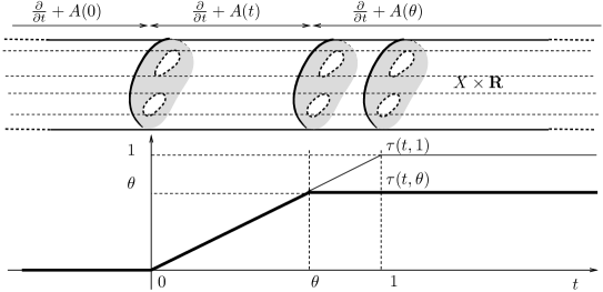
Figure 4: The operator $\mathcal{A}(\theta,\gamma)=\frac{\partial}{\partial t}+A(\tau(t,\theta))$ on the infinite cylinder $X\times\mathbf{R}$.

Lemma 1.

The operator $\mathcal{A}(\theta,\gamma)$ is Fredholm for $\theta$ such that $\gamma\notin\operatorname{Spec}(A(\theta)_{L})$, and $\operatorname{ind}\mathcal{A}(\theta,\gamma)$ is a locally constant function of $\theta$ on the set of such values of $\theta$.

Lemma 2.

If $\gamma,\widetilde{\gamma}\notin\operatorname{Spec}(A(\theta)_{L})$ and $\gamma>\widetilde{\gamma}$, then the difference $\operatorname{ind}\mathcal{A}(\theta,\widetilde{\gamma})-\operatorname{ind}\mathcal{A}(\theta,\gamma)$ is equal to the number of eigenvalues (counting multiplicities) of the operator $A(\theta)_{L}$ on the interval $(\widetilde{\gamma},\gamma)$.

Lemma 3.

$\operatorname{ind}\mathcal{A}(0,0)=0$.

Lemma 4.

$\operatorname{ind}\mathcal{A}(1,0)=\operatorname{ind}\bigl{(}\frac{\partial}{\partial t}+A(t)\bigr{)}_{\mathcal{L}}$.

The proof of Lemmas 1–4 will be given below. Now let us show that these lemmas imply the claim of the theorem. The spectral flow of the family $\{A(t)_{L}\}$ is given by Definition 1 for some partition $0=t_{0}<t_{1}<\dotsm<t_{n+1}=1$ and real numbers $\gamma_{1},\dots,\gamma_{n+1}=\gamma_{1}$, and we can assume that $\gamma_{1}=0$ (because we have assumed that $0\notin\operatorname{Spec}(A(0)_{L})$). Let $m_{j}$ be the number of eigenvalues (counting multiplicities) of the operator $A(t_{j})_{L}$ in the interval between $\gamma_{j}$ and $\gamma_{j+1}$. It follows from Lemma 1 that the operator $\mathcal{A}(\theta,\gamma_{j})$ is Fredholm for $\theta\in[t_{j-1},t_{j}]$ and

$$\operatorname{ind}\mathcal{A}(t_{j},\gamma_{j})-\operatorname{ind}\mathcal{A}(t_{j-1},\gamma_{j})=0,\qquad j=1,\dotsc,n+1.$$ (20)

By Lemma 2,

$$\operatorname{ind}\mathcal{A}(t_{j},\gamma_{j+1})-\operatorname{ind}\mathcal{A}(t_{j},\gamma_{j})=m_{j}\operatorname{sign}(\gamma_{j}-\gamma_{j+1}),\qquad j=1,\dotsc,n.$$ (21)

By summing relations (20) and (21) over all corresponding $j$, by adding the results, and by taking into account Lemma 3 and the relation $\gamma_{1}=\gamma_{n}=0$, we obtain

$$\operatorname{ind}\mathcal{A}(1,0)=\operatorname{ind}\mathcal{A}(1,0)-\operatorname{ind}\mathcal{A}(0,0)=\sum_{j=1}^{n}m_{j}\operatorname{sign}(\gamma_{j}-\gamma_{j+1})=\operatorname{sf}\{A(t)_{L}\}.$$ (22)

It remains to use Lemma 4. The proof of Theorem 2 is complete. ∎

Now let us prove Lemmas 1–4.

Proof of Lemma 1..

To prove that the operator $\mathcal{A}(\theta,\gamma)$ is Fredholm, it suffices to construct a regularizer, i.e., an operator

$$\mathcal{R}\colon L^{2}_{0\gamma}(X\times\mathbb{R},E)\longrightarrow\mathfrak{D}_{0\gamma}$$

such that the operators $I-\mathcal{A}(\theta,\gamma)\mathcal{R}$ and $I-\mathcal{R}\mathcal{A}(\theta,\gamma)$ are compact in the spaces $L^{2}_{0\gamma}(X\times\mathbb{R},E)$ and $\mathfrak{D}_{0\gamma}$, respectively. This can be done by the frozen-coefficients technique, standard in elliptic theory. (In our case, we “freeze” the variable $t$). To this end, for given $\tau\in[0,1]$ and $\nu\in\mathbb{R}$, consider the operator

$$\frac{\partial}{\partial t}+A(\tau)\colon L^{2}_{\nu\nu}(X\times\mathbb{R},E)\longrightarrow L^{2}_{\nu\nu}(X\times\mathbb{R},E)\quad\text{with domain $\mathfrak{D}_{\nu\nu}$.}$$ (23)

The operator (23) is invertible provided that $\nu\notin\operatorname{Spec}(A(\tau)_{L})$. The inverse operator $R_{\nu}(\tau)$ is given by the formula

$$[R_{\nu}(\tau)u](t)=\frac{1}{\sqrt{2\pi}}\int_{\operatorname{Im}p=\nu}e^{ipt}(ip+A(\tau)_{L})^{-1}\widetilde{u}(p)\,dp,\qquad u\in L^{2}_{\nu\nu}(X\times\mathbb{R},E),$$ (24)

where $\widetilde{u}(p)$, $\operatorname{Im}p=\nu$, is the Fourier transform of $u$ with respect to the variable $t$. Consider a finite cover $\{U_{j}\}_{j=1}^{s}$ of $[0,1]$ by open intervals such that $\nu_{j}\notin\operatorname{Spec}(A(\tau(t,\theta))_{L})$ for $t\in U_{j}$ for some real numbers $\nu_{j}$; let $U_{0}=(-\infty,0)$, $\nu_{0}=0$, $U_{s+1}=(1,\infty)$, and $\nu_{s+1}=\gamma$, and let $1=\sum_{j=0}^{s+1}\psi_{j}^{2}$ be a smooth partition of unity subordinate to the cover of the line $\mathbb{R}$ by the sets $U_{j}$, $j=0,\dotsc,s+1$. Then $\mathcal{R}$ can be defined by the formula

$$[\mathcal{R}u](t)=\sum_{j=0}^{s+1}\psi_{j}(t)\bigl{[}[\mathcal{R}_{\nu_{j}}(\tau)(\psi_{j}u)](t)\bigr{]}\big{|}_{\tau=\tau(t,\theta)}.$$

(Note that $\mathcal{R}$ is well defined as an operator from $L^{2}_{0\gamma}(X\times\mathbb{R},E)$ to $\mathfrak{D}_{0\gamma}$, because the operator of multiplication by $\psi_{j}$ is continuous from $L^{2}_{0\gamma}(X\times\mathbb{R},E)$ to $L^{2}_{\nu_{j}\nu_{j}}(X\times\mathbb{R},E)$ and from $\mathfrak{D}_{\nu_{j}\nu_{j}}$ to $\mathfrak{D}_{0\gamma}$. For $j\neq 0,s+1$, this follows from the compactness of the support of $\psi_{j}$; for $j=0$, from the fact that $\nu_{0}=0$ and $\psi_{0}(t)=0$ for $t>0$; for $j=s+1$, from the fact that $\nu_{s+1}=\gamma$ and $\psi_{s+1}(t)=0$ for $t<0$.) Now a straightforward computation shows that

$$\mathcal{A}(\theta,\gamma)\mathcal{R}u(t)=u(t)+\sum_{j=0}^{s+1}\biggl{[}\biggl{[}\biggl{(}\frac{\partial\psi_{j}}{\partial t}(t)\mathcal{R}_{\nu_{j}}(\tau)+\psi_{j}(t)\frac{\partial\tau}{\partial t}(t,\theta)\frac{\partial\mathcal{R}_{\nu_{j}}}{\partial\tau}(\tau)\biggr{)}(\psi_{j}u)\biggr{]}(t)\biggr{]}\bigg{|}_{\tau=\tau(t,\theta)}.$$

Since the functions $\frac{\partial\psi_{j}}{\partial t}(t)$ and $\frac{\partial\tau}{\partial t}(t,\theta)$ are compactly supported, it follows from standard facts about embeddings of Sobolev spaces that the second term on the right-hand side defines a compact operator on $L^{2}_{0\gamma}(X\times\mathbb{R},E)$. In a similar way, one can study the product $\mathcal{R}\mathcal{A}(\theta,\gamma)$.

The local constancy of the index of $\mathcal{A}(\theta,\gamma)$ as a function of $\theta$ follows from the fact that this operator continuously depends on $\theta$ in the operator norm as an operator from $\mathfrak{D}_{0\gamma}$ to $L^{2}_{0\gamma}(X\times\mathbb{R},E)$. The proof of Lemma 1 is complete. ∎

Proof of Lemma 3.

This lemma is the special case of the invertibility of the operator (23) for $\nu=0$ and $\tau=0$. ∎

The proof of Lemmas 2 and 4 is based on the localization method (the index locality principle; see [26, Theorem 4.10] and also [25, 23, 24] and the references therein). Having in mind our goals, let us state the claim of Theorem 4.10 in [26] for the simplest special case.

Let $N_{1},N_{2}\subset M$ be disjoint closed subsets of a manifold $M$, and let $D\colon\mathcal{H}_{1}\longrightarrow\mathcal{H}_{2}$ be a bounded Fredholm operator acting on some Hilbert spaces of sections of bundles over $M$. Next, let $\varkappa\colon M\to[0,1]$ be a smooth mapping such that $N_{1}\subset f^{-1}(0)$ and $N_{2}\subset f^{-1}(1)$, and let $\mathcal{C}\subset C^{\infty}(M)$ be a subalgebra consisting of functions constant on $N_{1}$ and on $N_{2}$ and containing all functions of the form $\psi(x)=\varphi(\varkappa(x))$, where $\varphi$ is a smooth function on $[0,1]$. Suppose that the commutator of $D$ with the operator of multiplication by any function in $\mathcal{C}$ is compact. Then the index increments arising from changes of $D$ on $N_{1}$ and $N_{2}$ preserving the Fredholm property and the compactness of commutators are independent:

$$\Delta_{N_{1}\sqcup N_{2}}=\Delta_{N_{1}}+\Delta_{N_{2}},$$

where

• $\Delta_{N_{1}}$ is the index increment occurring if the operator is changed only on $N_{1}$.

• $\Delta_{N_{2}}$ is the index increment occurring if the operator is changed only on $N_{2}$.

• $\Delta_{N_{1}\sqcup N_{2}}$ is the index increment occurring if the operator is simultaneously changed both on $N_{1}$ and $N_{2}$.

The practical application of the localization method to the proof of Lemmas 2 and 4 implements the following idea. We wish to compute how the index of some operator $D$ changes for a given change of the operator on a set $N_{1}$, but it is difficult to compute the index increment owing to the complicated structure of $D$ outside $N_{1}$. Let us modify the operator $D$ on some set $N_{2}$ disjoint with $N_{1}$ so as to obtain an operator $\widetilde{D}$ of simpler structure whose index increment under the given change on $N_{1}$ can be computed. This increment coincides with the desired increment for the original operator.

Proof of Lemma 2.

Take $X\times\mathbb{R}$ for the manifold $M$, the set $\{t\geq 2\}$ for $N_{1}\subset M$, the set $\{t\leq 1\}$ for $N_{2}\subset M$, and the algebra of infinitely differentiable functions $\varphi(t)$ of $t\in\mathbb{R}$ constant on $N_{1}$ and on $N_{2}$ for the function algebra $\mathcal{C}$. The original operator $D$ is the operator $A(\theta,\gamma)$, which we treat as a bounded Fredholm operator on the spaces

$$D=A(\theta,\gamma)\colon\mathfrak{D}_{0\gamma}\longrightarrow L_{0\gamma}^{2}(X\times\mathbb{R},E),$$ (25)

and we need to compute the index increment for this operator if $\gamma$ is replaced by $\widetilde{\gamma}$. Note that the commutator of the operator (25) with a smooth function $\varphi\in\mathcal{C}$ is the operator of multiplication by the compactly supported function $\varphi^{\prime}(t)$, which is compact as an operator from $\mathfrak{D}_{0\gamma}$ to $L_{0\gamma}^{2}(X\times\mathbb{R}^{1},E)$, so that we are just in a position to use the localization method. The replacement of $\gamma$ by $\widetilde{\gamma}$ changes the operator $D$ only on the set $N_{1}$. (The expression specifying the operator and the boundary conditions remain the same, but the spaces where the operator acts are changed, the change being solely concerned with the admissible growth of functions as $t\to+\infty$; i.e., in particular, the restriction of these spaces to $M\setminus N_{1}$ is unchanged at all.) Now let us replace $D$ by the operator

$$\widetilde{D}=\frac{\partial}{\partial t}+A(\theta)\colon\mathfrak{D}_{\gamma\gamma}\longrightarrow L_{0\gamma}^{2}(X\times\mathbb{R},E).$$ (26)

This operator differs from $D$ (both in the differential expression and in the spaces where it acts) only on $N_{2}$. Thus, it suffices to compute the index increment for this operator under the change on $N_{1}$ the same as for $D$. The operator $\widetilde{D}$ is invertible, so that $\operatorname{ind}\widetilde{D}=0$. The change of this operator on $N_{1}$ results in the operator

$$\frac{\partial}{\partial t}+A(\theta)\colon\mathfrak{D}_{\gamma\widetilde{\gamma}}\longrightarrow L^{2}_{\gamma\widetilde{\gamma}}(X\times\mathbb{R},E);$$ (27)

thus, it remains to compute the index of the latter. For this computation, it is convenient to treat the operator (27) as an unbounded Fredholm operator on $L^{2}_{\gamma\widetilde{\gamma}}(X\times\mathbb{R},E)$ with domain $\mathfrak{D}_{\gamma\widetilde{\gamma}}$. Then the adjoint operator has the form $-\frac{\partial}{\partial t}+A(\theta)$ and acts on the dual space $L^{2}_{-\gamma,-\widetilde{\gamma}}(X\times\mathbb{R},E)$ with domain $\mathfrak{D}_{-\gamma,-\widetilde{\gamma}}$. The elements of the null space of the operator (27) should have the form $v(x)e^{-\lambda t}$, where $\lambda$ is an eigenvalue of $A(\theta)_{L}$ and $v(x)$ is one of the corresponding eigenfunctions. The condition that these elements belong to the weighted space $L^{2}_{\gamma\widetilde{\gamma}}(X\times\mathbb{R},E)$ implies that $\widetilde{\gamma}<\lambda<\gamma$. Thus, the dimension of the null space is equal to the number of eigenvalues (with regard of multiplicity) of the operator $A(\theta)_{L}$ in the interval $(\widetilde{\gamma},\gamma)$. The elements of the null space of the adjoint operator should have the form $v(x)e^{\lambda t}$ and belong to the weighted space $L^{2}_{-\gamma,-\widetilde{\gamma}}(X\times\mathbb{R},E)$). It follows that $\gamma<\lambda<\widetilde{\gamma}$, but this is impossible, because $\gamma>\widetilde{\gamma}$. Thus, the null space of the adjoint operator is trivial, the index of the operator (27) coincides with the dimension of its null space, and we arrive at the assertion of Lemma 2. ∎

Proof of Lemma 4.

We need to prove that the operators

$$\mathcal{A}(1,0)\colon\mathfrak{D}_{00}\longrightarrow L^{2}(X\times\mathbb{R},E)$$ (28)

and

$$\biggl{(}\frac{\partial}{\partial t}+A(t)\biggr{)}_{\mathcal{L}}\colon\mathfrak{D}_{\mathcal{L}}\longrightarrow L^{2}(X\times S^{1},\mathcal{E})$$ (29)

have the same index. We assume (this can always be achieved by a homotopy) that $A(t)=A(1)$ for $t\geq 1-2\varepsilon$ and $A(t)=A(0)$ for $t\leq 2\varepsilon$ for some given $\varepsilon>0$. Set

$$N_{1}=\{t\in(-\infty,\varepsilon]\cup[1-\varepsilon,\infty)\},\qquad N_{2}=\{t\in[2\varepsilon,1-2\varepsilon]\}.$$

For the function algebra $\mathcal{C}$ we again take the algebra of infinitely differentiable functions $\varphi(t)$ of $t$ constant on $N_{1}$ and $N_{2}$. The operator (29) can be obtained from the operator (28) by the following change on $N_{1}$: one cuts away and disposes of the half-cylinders $X\times(-\infty,0)$ and $X\times(1,\infty)$, and the faces $X\times\{0\}$ and $X\times\{1\}$ of the remaining product $X\times[0,1]$ are glued together, the bundle $E$ giving rise to the bundle $\mathcal{E}$ via the clutching automorphism $U\colon E|_{t=0}\longrightarrow E|_{t=1}$.

We should show that the index increment for this change of the operator on $N_{1}$ is zero. To this end, we replace the operator (28) by the operator

$$\mathcal{A}(0,0)\colon\mathfrak{D}_{00}\longrightarrow L^{2}(X\times\mathbb{R},E).$$ (30)

The operator (30) will differ from the operator (28) only on $N_{2}$ if we rewrite the former in the equivalent form

$$\mathcal{A}(0,0)=\begin{cases}\frac{\partial}{\partial t}+A(0)&\text{for $t\leq\frac{1}{2}$,}\\ \frac{\partial}{\partial t}+A(1)&\text{for $t\geq\frac{1}{2}$,}\end{cases}$$ (31)

where it is assumed that the bundle in which the operator (31) acts is obtained from $E|_{t\leq\frac{1}{2}}$ and $E|_{t\geq\frac{1}{2}}$ by the standard clutching construction at $t=\frac{1}{2}$ with the automorphism

$$U^{-1}\colon E|_{t=1/2+0}\longrightarrow E|_{t=1/2-0}.$$

(The passage from (30) to (31) is essentially none other than rewriting the operator $\mathcal{A}(0,0)$ for $t\geq\frac{1}{2}$ in “new coordinates” in the fibers of $E$.)

Now let us change the operator (30) written in the form (31) on $N_{1}$ in the same way as we have earlier changed the operator (28). The resulting operator on $X\times S_{1}$ has the form (31), and the bundle in which it acts is obtained from $E$ by clutching construction with the automorphism

$$U\colon E|_{t=0}\longrightarrow E|_{t=1},\qquad U^{-1}\colon E|_{t=1/2+0}\longrightarrow E|_{t=1/2-0}.$$

It is easily seen that this bundle is isomorphic to the pullback of $E$ on $X\times S_{1}$, and the resulting operator itself is none other than $\bigl{(}\frac{\partial}{\partial t}+A(0)\bigr{)}_{L}$; its index is zero, because it is invariant with respect to rotations along $S^{1}$. The index of the operator (28) is zero as well (it is invertible), so that the index increment is zero, and the proof of the lemma is complete. ∎

Proof of Theorem 1.

Theorem 2 shows that the spectral flow of the family (2) obeys the localization principle: any modifications applied to the Dirac operator (1) in the planar domain $X$ and to the function $B$ occurring in the boundary conditions automatically lift to $X\times S_{1}$ becoming modifications of $\frac{\partial}{\partial t}+D_{t}$; the latter enjoy the index locality principle [26, Theorem 4.10], and the index is equal to the spectral flow by Theorem 2.

Figure 5: Cutting a domain with holes into pieces.

Figure 6: Cutting a domain without holes into pieces.

The localization principle permits one to split the domain with holes into parts with fewer holes. Let us show this by example. Figure 5, left shows a domain $X$ with two holes. Let us reduce the computation of the spectral flow of a family of Dirac operators with local boundary conditions in $X$ to the corresponding computation for domains with one hole. Let $N_{1}$ be the set dashed in Fig. 5, left, and let $N_{2}$ be the complement to a small neighborhood of $N_{1}$. Let us change the domain inside $N_{1}$ as shown in Fig. 5, right, so that the original domain becomes two domains with smooth boundary. The function $B(x)$ occurring in the boundary conditions can be extended by continuity as a nonvanishing real-valued function to the newly arising boundary arcs inside $N_{1}$, because the sign of $B(x)$ is the same on the entire outer boundary of the original domain. Thus, the domain splits into two unrelated parts, and to prove that the spectral flow of the family of Dirac operators in the original domain is equal to the sum of spectral flows corresponding to the two new domains, one should show that the increment of the spectral flow under this modification of the domain is zero. To this end, we use the localization method. Let us change the original family by changing the domain in $N_{2}$ (so that the resulting domain has the form shown in Fig. 6, left) and by extending $B(x)$ by continuity as a nonvanishing function to the newly arising boundary arcs inside $N_{2}$. The spectral flow of the new family is zero before as well as after the modification shown in Fig. 6, because the domains in this figure are contractible and the gauge transformation $\mu$ in these domains is homotopic to the identity transformation. Thus, cutting the domain into pieces reduces the problem to the case of domains with one hole, for which formula (3) was proved in [20]. (Needless to say, one can prove it directly with the use of Theorem 2, but there is no need to do this, and we omit the corresponding computations for lack of space.) ∎

5. CONCLUSIONS

Let us discuss possible physical realizations of nonzero spectral flow. We start with the case of graphene. One has to keep in mind that there are two Dirac electron subsystems in graphene (two valleys) and, generally speaking, scattering at the edges mixes the two valleys [7, 31]. This is not the case, however, if an energy gap in the electron energy spectrum opens smoothly when reaching the edge. At the chemical functionalization of the edges this is, indeed, the case, since electronic structure is modified in a sufficiently large region of space [32]. As a result, intervalley scattering is negligible and we have the boundary condition (1) suggested first by Berry and Mondragon [19]. A detailed microscopic derivation of the boundary condition starting with a discrete lattice model has been done in Ref. [31] (see also [7, Chapter 5] and references therein). The sign of the constant $B$ is determined by the sign of the mass term in the Dirac equation and is dependent on the distribution of chemical groups along the edge. One can hope that if we prepare graphene rings, then in some specimens the signs of $B$ will be opposite at the internal and external edges of the ring, which is necessary for nonzero spectral flow. However, it is hard to reach in a controllable way.

Probably, topological insulators are more promising in this sense. First, two-dimensional massless Dirac fermions are realized at the surface of three- dimensional topological insulators, such as $\operatorname{Bi}_{2}\operatorname{Se}_{3}$, only one Dirac cone arising [8, 9]. To open the gap, one has to cover the surface by a magnetic layer, the sign of the gap being determined by the direction of magnetization [8, 9]. This opens a way to manipulate the sign of the constant $B$. Second, two-dimensional massless Dirac fermions can be realized in a layer of $\operatorname{HgTe}$ confined between two layers of $\operatorname{CdTe}$, at a certain critical thickness of the layer [8, 9]. Recently, such an opportunity has been demonstrated experimentally [33]. If the thickness of the layer varies smoothly in space oscillating near the critical value, one can reach both positive and negative values of $B$. Currently, this opportunity to create nonzero spectral flow looks the most promising.

Acknowledgments.

The second author’s research was supported by the Russian Foundation for Basic Research (grant no. 11-01-00973). The authors are grateful to S. Yu Dobrokhotov and A. I. Shafarevich for attention and useful discussion.

References

- [1] N. D. Mermin, Rev. Mod. Phys., 51 (1979), 591.
- [2] D. J. Thouless, M. Kohmoto, M. P. Nightingale, and M. den Nijs, Phys. Rev. Lett., 49 (1982), 405.
- [3] J. Bellisard, A. van Elst, and H. Schulz-Baldes, J. Math. Phys., 35 (1994), 5373.
- [4] F. Wilczek, Fractional Statistics and Anyon Superconductivity, World Scientific, Singapore, 1990.
- [5] G. E. Volovik, The Universe in a Helium Droplet, Clarendon, Oxford, 2003.
- [6] M. A. H. Vozmediano, M. I. Katsnelson, and F. Guinea, Phys. Rep., 496 (2010), 109.
- [7] M. I. Katsnelson, Graphene. Carbon in Two Dimensions, Cambridge University Press, Cambridge, 2012.
- [8] M. Z. Hasan and C. L. Kane, Rev. Mod. Phys., 82 (2010), 3045.
- [9] X.-L. Qi and S.-C. Zhang, Rev. Mod. Phys., 83 (2011), 1057.
- [10] M. F. Atiyah and I. M. Singer, Bull. Amer. Math. Soc., 69 (1963), 422.
- [11] N. B. Kopnin, Rep. Prog. Phys., 65 (2002), 1633.
- [12] Y. Aharonov and D. Bohm, Phys. Rev., 115 (1959), 485.
- [13] S. Olariu and I. I. Popescu, Rev. Mod. Phys., 57 (1985), 339.
- [14] Y. Avishai, Y. Hatsugai, and M. Kohmoto, Phys. Rev. B, 47 (1993), 9501.
- [15] P. Recher et al., Phys. Rev. B, 76 (2007), 235404.
- [16] R. Jackiw, A. I. Milstein, S.-Y. Pi, and I. S. Terekhov, Phys. Rev. B, 80 (2009), 033413.
- [17] M. I. Katsnelson, Europhys. Lett., 89 (2010), 17001.
- [18] M. Atiyah, V. Patodi, and I. Singer, Math. Proc. Cambridge Philos. Soc., 79 (1976), 71.
- [19] M. Berry and R. J. Mondragon, Proc. R. Soc. London A, 412 (1987), 53.
- [20] M. Prokhorova, The spectral flow for Dirac operators on compact planar domains with local boundary conditions, Max Planck Institute for Mathematics Preprint Series, no. 76, 2011, arXiv:1108.0806v2.
- [21] M. Atiyah and R. Bott, “The index problem for manifolds with boundary”, Bombay Colloquium on Differential Analysis, Oxford University Press, Oxford, 1964, 175.
- [22] L. Hörmander, The Analysis of Linear Partial Differential Operators, Vol. 3, Springer-Verlag, Berlin, 1985.
- [23] V. E. Nazaikinskii and B. Yu. Sternin, Dokl. Ross. Akad. Nauk, 370 (2000), 19.
- [24] V. E. Nazaikinskii and B. Yu. Sternin, Funct. Anal. Appl., 35:2 (2001), 111.
- [25] V. E. Nazaikinskii and B. Yu. Sternin, Abstract and Applied Analysis (2006), Article ID 98081.
- [26] V. Nazaikinskii, A. Savin, B.-W. Schulze, and B. Sternin, Elliptic Theory on Singular Manifolds, CRC Press, Boca Raton, 2005.
- [27] B. Booß-Bavnbek, M. Lesch, and J. Phillips, Canad. J. Math., 57 (2005), 225.
- [28] B. Booß-Bavnbek and K. Wojciechowski, Elliptic Boundary Problems for Dirac Operators, Birkhäuser, Boston–Basel–Berlin, 1993.
- [29] J. Brüning and M. Lesch, J. Funct. Anal., 185 (2001), 1.
- [30] B. Booß-Bavnbek, M. Lesch, and C. Zhu, J. Geom. Phys., 59 (2009), 784.
- [31] A. R. Akhmerov and C. W. J. Beenakker, Phys. Rev. B, 77 (2008), 085423.
- [32] D. W. Boukhvalov and M. I. Katsnelson, Nano Lett., 8 (2008), 4373.
- [33] B. Büttner et al., Nature Physics, 7 (2011), 418.