Darcy’s flow with prescribed contact angle – Well-posedness and lubrication approximation

Abstract.

We consider the spreading of a thin two-dimensional droplet on a solid substrate. We use a model for viscous fluids where the evolution is governed by Darcy’s Law. At the triple point where air and liquid meet the solid substrate, the liquid assumes a constant, non-zero contact angle (partial wetting). We show local and global well-posedness of this free boundary problem in the presence of the moving contact point. Our estimates are uniform in the contact angle assumed by the liquid at the contact point. In the so-called lubrication approximation (long-wave limit) we show that the solutions converge to the solution of a one-dimensional degenerate parabolic fourth order equation which belongs to a family of thin-film equations. The main technical difficulty is to describe the evolution of the non-smooth domain and to identify suitable spaces that capture the transition to the asymptotic model uniformly in the small parameter $\epsilon$.

.

1. Introduction and model

In the past years, the theory of fluid systems in the presence of a free boundary has been developed by many important works. Usually, in these problems, the interface (or free boundary) separates two phases of the fluid system. Among the large literature, such work has been addressed e.g. in [31, 30, 13, 39, 44, 12] for local existence results, [42, 19] for global existence results, [10] for the study of blow-up, [2, 32] for asymptotic limits. In this paper, we are interested in the situation of a fluid evolution in the presence of a contact point where three phases meet, namely a contact point between air, liquid and solid, see Fig. 1. One example is the flow in a Hele-Shaw cell, where the liquid touches the lateral boundary of the Hele-Shaw cell.

The Hele-Shaw model describes the evolution of a liquid between the plates of a Hele-Shaw cell. In general, the surface tension-driven Hele-Shaw flow is given by

$$\left\{\begin{aligned} &\Delta p\ =\ 0\qquad\qquad&&\text{in $\Omega(t)$},\\ &p\ =\ \gamma\kappa&&\text{on $\partial\Omega(t)$},\\ &V\ =\ \nabla p\cdot n&&\text{on $\partial\Omega(t)$},\end{aligned}\right.$$ (1.1)

where the evolving domain $\Omega(t)\subset\mathbb{R}^{2}$ describes the region occupied by the fluid. The velocity of the fluid is described by Darcy’s Law $U=-\nabla p$. In particular the normal velocity $V$ of the fluid interface is described by $V=\nabla p\cdot n$. The parameter $\gamma$ describes the surface tension between air and liquid. Next to its interpretation as the flow in a Hele-Shaw cell, the fluid evolutions governed by Darcy’s Law appear in a wide range of physical models. One example is the flow of a liquid through a porous medium, see [6]. Other situations which can be modeled by (1.1) are crystal growth or dissolution, directional solidification or melting, electrochemical machining or forming [41, 38, 33]. In the last two decades, well-posedness of (1.1) has been investigated: Short-time existence and regularity of solutions of (1.1) have been proved in [15, 24, 17, 18] and Prokert [35]. Global existence for initial data close to the sphere has been shown in [11]. The case of zero surface tension, $\gamma=0$ has been considered e.g. in [40, 1].

Clearly, the normal component of the velocity is zero at the liquid-solid interface. We assume that the Hele-Shaw cell is described by the half-space $H=\mathbb{R}\times(0,\infty)$. At the point where air, liquid and solid meet, we assume that the liquid assumes a static (microscopic) contact angle. This contact angle $\theta$ is determined by Young’s Law [43], i.e. $\gamma\cos\theta\ =\ \gamma_{SG}-\gamma_{SL}$ where the parameter describe the surface tensions between the three phases: $\gamma$ (air, liquid), $\gamma_{SL}$ (solid, liquid) and $\gamma_{SG}$ (air, solid). This leads to the following model:

$$\left\{\begin{aligned} &\Delta p\ =\ 0\qquad&&\text{in }\Omega(t),\\ &p\ =\ \gamma\kappa&&\text{on }\partial\Omega(t)\cap H,\\ &p_{y}\ =\ 0&&\text{on }\partial\Omega(t)\cap\partial H,\\ &\gamma\cos\theta\ =\ \gamma_{SG}-\gamma_{SL}\qquad\qquad&&\text{on }\partial(\partial\Omega(t)\cap\partial H),\end{aligned}\right.$$ (1.2)

see Fig. 1. The evolution then can also be interpreted as the spreading of a droplet on a plate. A well-posedness result for (1.2) in Hölder spaces has been given by Bazalyi and Friedman in [5, 4]. However, in their analysis the conditions on the initial data are too restrictive to allow for movement of the triple point (and thus for spreading of the droplet). Our first main result is a well-posedness result for this free boundary problem in a much wider class of weighted Sobolev spaces. In particular, our result seems to be the first result which allows for movement of the triple point.

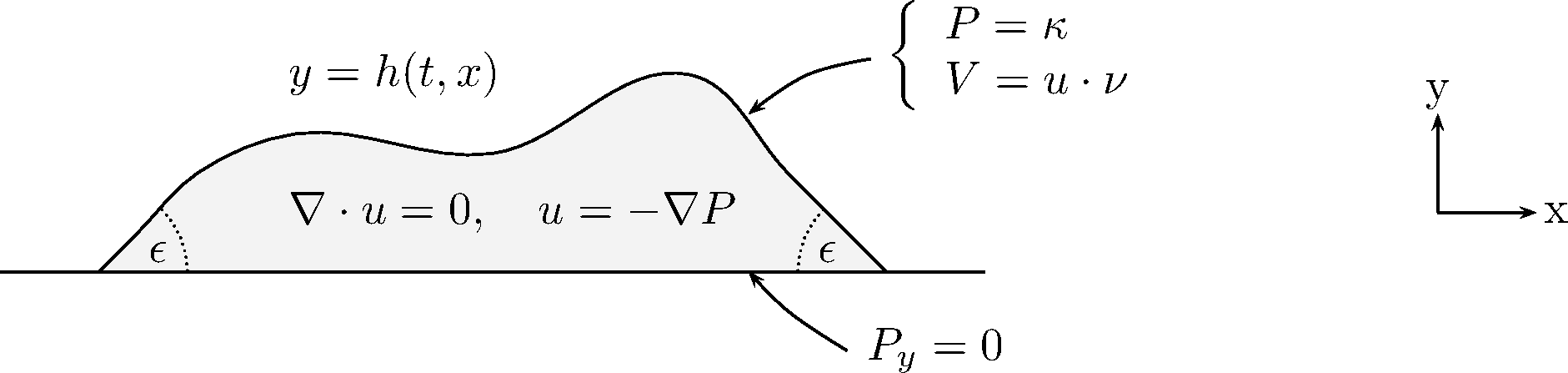
Figure 1. Darcy flow on solid substrate

The second aim of this work is to show the convergence of solutions to a reduced model in the so called lubrication approximation regime or long wave approximation. More precisely, let us assume that typical vertical length scales are of order $\epsilon$ while horizontal length scales are of order $1$. In particular, the angle assumed at the contact point is of order $\epsilon$:

$$\frac{\epsilon^{2}}{2}\ \simeq\ \frac{\theta^{2}}{2}\ \simeq\ 1-\cos\theta\ =\ \frac{\gamma+\gamma_{SL}-\gamma_{SG}}{\gamma}.$$ (1.3)

The limit model is a special form of the thin-film equation. Assuming that the height of the droplet is described by the graph $h(t,x)$, the evolution is given by

$$\left\{\begin{aligned} &h_{t}+\gamma(hh_{xxx})_{x}=0\qquad&&\text{in }\{h>0\},\\ &h=0,\quad|h_{x}|=\epsilon,\qquad&&\text{on }\partial\{h>0\},\\ &\tilde{V}=\gamma h_{xxx}\qquad&&\text{on }\partial\{h>0\}\end{aligned}\right.$$ (1.4)

and where $\tilde{V}$ is the velocity of the moving contact points $\partial\{h>0\}$. Formal derivations of lubrication models of type (1.4) have been e.g. given in [37]. We prove convergence of solutions of (1.2) to solutions of (1.4). This is the first rigorous lubrication approximation in the case of partial wetting (non-zero contact angle). Furthermore, it is the first convergence result in the framework of classical solutions. A rigorous lubrication approximation in the framework of weak solutions has been done by Giacomelli and Otto [23]. Their approach is quite different to ours: In particular, their result does not include well-posedness for the initial model. Instead, the authors prove convergence to the limit model by only minimal energy bounds, assuming existence of smooth solutions. In particular, the bounds derived in [23] do not capture the slope of the profile at the contact point. Indeed, the techniques used in [23] do not seem to be applicable for the case of a non-zero contact angle at the moving contact line as considered in this work.

The main work lies in the derivation of bounds which are uniform in the parameter $\epsilon>0$. We give a short sketch of the strategy of our proof: In order to perform the transition from (1.2) to (1.4), we first express (1.2) as a nonlocal evolution problem in terms of the profile function $h(t,x)$. The corresponding equation can be seen as a nonlocal parabolic evolution problem of third order. Equation (1.4) on the other hand is a local fourth order degenerate parabolic equation. As the considered models are higher order equations, the maximum principle cannot be used. Instead we rely on their dissipative structures. Indeed, solutions of (1.2) satisfy

$$\,\frac{d}{dt}\big{(}(|\partial\Omega\cap H|)-\alpha|\partial\Omega\cap\partial H)\big{)}\ =\ -\frac{1}{\gamma}\int\!\!\!\!\int_{\Omega(t)}|\nabla p|^{2}\ dxdy,$$ (1.5)

where $\alpha=\cos(\arctan\epsilon)$, see e.g. [22]. The dissipation relation for solutions of (1.4) is

$$\,\frac{d}{dt}\big{(}\int_{\mathbb{R}}h_{x}^{2}\ dx+\epsilon^{2}|\{h>0\}|\big{)}\ =\ -\gamma\int_{\mathbb{R}}hh_{xxx}^{2}\ dx.$$ (1.6)

One of the core issues of the analysis is to find suitable norms which allow for uniform bounds in the limit $\epsilon\to 0$. In [26], we have investigated the linearizations of (1.2) and (1.4). The analysis in this work suggests to use sums of weighted Sobolev norms of the type

$$[f]_{X_{\epsilon}^{k}}\ =\ \inf_{f=f_{+}+f_{-}}\big{(}\|x^{k+\delta}\partial_{x}^{4k+\delta}f_{+}\|_{L^{2}}+\|{\textstyle(\frac{1}{\epsilon})^{k}}x^{\delta}\partial_{x}^{3k+\delta}f_{-}\|_{L^{2}}\big{)}.$$ (1.7)

where $f=h_{x}-1$ and where $k,\delta\geq 0$. In the limit $\epsilon\to 0$, this norm turns from a sum of weighted Sobolev norms of order $4k+\delta$ and $3k+\delta$ to a weighted Sobolev norm of order $4k+\delta$ (first term on the right hand side of (1.7)). This transition in the character of the norm is reflected by a transition in the character of the equation: In the limit $\epsilon\to 0$, the model (understood as an evolution equation for the profile function, cf. (2.25), (2.28)) changes

• from a third order to a fourth order evolution equation and

• from a non-degenerate parabolic to a degenerate parabolic equation.

In particular, we will use norms of type (1.7) with $\delta=1$. This seems to be the smallest integer value that is sufficient to control the nonlinearity of the problem (the norms (1.7) are stronger for larger $\delta$ as follows from Hardy’s inequality). We also need to choose norms which control the pressure $p$. As we will see, the norms for the pressure do not have a real space representation, but are rather described in terms of the Mellin transformed function. In fact, the choice of suitable norms for the pressure turns out to be delicate in order to obtain uniform bounds in the small $\epsilon$ parameter. We use radial variables with respect to the moving contact point at the origin of the coordinate system. The norms, we use are weighted Sobolev norms of supremum-type in the angular direction (in real space variables) and of $L^{2}$-type in radial direction (in frequency variables).

Structure of the paper: In Section 2, we transform the problem on a fixed domain and we define the norms to control the profile and the pressure. The main results of this work are stated and discussed in Section 3. In Section 4, we give an overview for the proofs of the main theorems. In Section 5, we prove estimates for weighted spaces. In Section 6, we derive estimates for the nonlinear operator for a droplet supported in half-space. In Section 7, we derive corresponding localized estimates for compactly supported droplets.

2. Setting and norms

By a change of dependent and independent coordinates, we reformulate the problem on a fixed domain. We then formulate (1.2) as a nonlocal evolution equation in terms of the profile function $h$. We also introduce norms to control profile and pressure.

2.1. Transformation onto a fixed domain

We define the nonlinear operator ${\mathcal{B}}^{h}$ of Dirichlet-Neumann type by

$${\mathcal{B}}^{h}\kappa(x)\ =\ \sqrt{1+h_{x}^{2}}\ \left(\partial_{n}p\right)_{|y=h(t,x)}, \left\{\begin{array}[]{ll}\Delta p=0&\text{in $\Omega(t)$},\\ p=\gamma\kappa&\text{on $\partial_{1}\Omega(t)$},\\ p_{y}=0&\text{at $\partial_{0}\Omega(t)$},\end{array}\right.$$ where (2.4)

where $\partial_{1}\Omega(t):=\partial\Omega(t)\cap\{y>0\}$ and $\partial_{0}\Omega(t):=\partial\Omega(t)\cap\{y=0\}$ With the assumption that the free boundary moves with the velocity, we have $h_{t}=w-vh_{x}$, where $u=(v,w)$ is the velocity of the liquid. Suppose that the support of the droplet stays an interval for some time, i.e. $\operatorname*{supp}h(t)=(s_{-}(t),s_{+}(t))$ for $t\in(0,\tau)$. The evolution (1.2) can then be equivalently written as nonlocal evolution for the profile $h$ by

$$h_{t}+{\mathcal{B}}^{h}\kappa=0,\qquad \text{for }x\in(s_{-}(t),s_{-}(t))$$ (2.5)

with boundary conditions $h_{|x=s_{\pm}}=0$, $|h_{x|x=s_{\pm}}|=\epsilon$ and $\dot{s}_{\pm}(t)=-\kappa_{x|x=s_{\pm}}$. By (2.4) and since $|h_{x}|=\epsilon$ at the triple point, the movement of the triple point is given by

$$\partial_{t}s_{\pm}=-p_{x|x=s_{\pm}}=-\gamma\kappa_{x|x=s_{\pm}}\ =\gamma\Big{(}(1+\epsilon^{2})^{-\frac{3}{2}}\ h_{xxx}-3\epsilon(1+\epsilon^{2})^{-\frac{5}{2}}\ h_{xx}^{2}\Big{)}_{|x=s_{\pm}}.$$ (2.6)

Indeed, (2.6) follows since $p(t,x,h(t,x))=\kappa(t,x)$ and hence $p_{x}+h_{x}p_{y}=\kappa_{x}$ at $x=s(t)$ and we conclude since $p_{y}=0$ for $y=0$. We will assume that the support of $h$ at initial time is given by $(0,1)$. We next rescale time and space to get ${\mathcal{O}}(1)$ quantities; furthermore we fix the position of the moving contact point $s(t)$ by using moving coordinates: We set

$$M(t)\ =\ \tfrac{1}{2}(s_{+}(t)+s_{-}(t)), D(t)\ =\ s_{+}(t)-s_{-}(t).$$ (2.7)

We introduce the new variables $(\tilde{x},\tilde{y},\tilde{t})$ by

$$\tilde{x}\ =\ \frac{x-M(t)}{D(t)}+\frac{1}{2}, \tilde{y}\ =\ \frac{y}{\epsilon D(t)}, \tilde{t}\ =\ \epsilon\gamma\int_{0}^{t}\frac{1}{D^{2}(s)}\ ds,$$ (2.8)

cf. [3, 20]. In particular, $\partial_{x}\tilde{x}=\frac{1}{D}$, $\partial_{x}\tilde{t}=0$, $\partial_{t}\tilde{t}=\frac{\epsilon\gamma}{D^{2}}$ and

$$\partial_{t}\tilde{x}\ =\ -\frac{M_{t}}{D}-\frac{D_{t}(x-M)}{D^{2}}\stackrel{{\scriptstyle\eqref{newcoord}}}{{=}}-\frac{\epsilon\gamma}{D^{3}}\big{(}\dot{M}+(\tilde{x}-{\frac{1}{2}})\ \dot{D}\big{)}\stackrel{{\scriptstyle\eqref{def-MD}}}{{=}}\ -\frac{\epsilon\gamma}{D^{3}}\big{(}(1-\tilde{x})\dot{s}_{-}+x\dot{s}_{+}\big{)},$$

where the dot denotes differentiation in $\tilde{t}$. The dependent quantities $\tilde{h}$ and $\tilde{p}$ are defined by

$$h(t,x)=\epsilon D(t)\tilde{h}(\tilde{t},\tilde{x}), D(t)p(t,x,y)=\epsilon\gamma\tilde{p}(\tilde{t},\tilde{x},\tilde{y}).$$ (2.9)

The transformed evolution — after multiplication by $D^{2}/\epsilon\gamma$ — is given by

$$\big{(}D\tilde{h}\big{)}_{\tilde{t}}-\big{(}(1-x)\dot{s}_{-}+x\dot{s}_{+}\big{)}\ h_{\tilde{x}}-{\mathcal{B}}_{\epsilon}^{\tilde{h}}\big{(}(1+\epsilon^{2}{\tilde{h}}_{\tilde{x}}^{2})^{-\frac{3}{2}}\tilde{h}_{\tilde{x}\tilde{x}}\big{)}\ =\ 0 x\in(0,1)$$ for (2.10)

with boundary conditions $h=0$ and $|h_{x}|=1$ at $x=0,1$. The operator ${\mathcal{B}}_{\epsilon}^{h}$ is given by

$${\mathcal{B}}_{\epsilon}^{\tilde{h}}\eta(\tilde{x})\stackrel{{\scriptstyle\eqref{B-phys}}}{{=}}\left(-{\tilde{h}}_{\tilde{x}}\tilde{p}_{\tilde{x}}+({\textstyle\frac{1}{\epsilon}})^{2}{\tilde{p}}_{\tilde{y}}\right)_{|\tilde{y}=\tilde{h}(\tilde{t},\tilde{x})}, \left\{\begin{array}[]{ll}\Delta_{\epsilon}\tilde{p}=0&\text{in }\tilde{\Omega},\\ \tilde{p}=\eta&\text{on }\partial_{1}\tilde{\Omega},\\ {\tilde{p}_{\tilde{y}}}=0&\text{on }\partial_{0}\tilde{\Omega}\end{array}\right.$$ where (2.14)

and where $\Delta_{\epsilon}=\partial_{x}^{2}+{\textstyle(\frac{1}{\epsilon})^{2}}\partial_{y}^{2}$. Here, $\tilde{\Omega}=\{((\tilde{x},\tilde{y}):\tilde{x}\in(0,1),\tilde{y}\in(0,\tilde{h}(t,x)))\}$. We will also use the notation $\tilde{\Gamma}=\partial_{1}\tilde{\Omega}$ for the air-liquid interface and $\Gamma_{0}=\partial_{0}\tilde{\Omega}=(0,1)$ for the liquid-solid interface. By Proposition 6.7, ${\mathcal{B}}_{\epsilon}^{h}$ is well-defined. In the following, we skip the tilde’s in our notation. Let $h^{*}=x(1-x)$ and let $f^{*}=h^{*}_{x}=1-2x$. Note that $h^{*}$ is an approximation of the stationary solution for the Darcy flow which is the half-circle. We set $f=(h-h^{*})_{x}=h_{x}-f^{*}$. We also use the notation $B_{\epsilon}^{f}:={\mathcal{B}}_{\epsilon}^{h}$. This yields the following evolution model, defined on the fixed domain $Q_{\tau}:=(0,\tau)\times(0,1)$,

$$\left\{\begin{aligned} &{\mathcal{L}}_{\epsilon}f:=(Df)_{t}-\Big{[}\big{(}(1-x)\dot{s}_{-}+x\dot{s}_{+}\big{)}(f+f^{*})+B_{\epsilon}^{f}\Big{(}\frac{f_{x}+f_{x}^{*}}{(1+\epsilon^{2}(f-2)^{2})^{\frac{3}{2}}}\Big{)}\Big{]}_{x}=0,\\ &f=0\hskip 38.74988pt\text{at }x=0,1,\\ &\int_{0}^{1}f\ dx=0.\end{aligned}\right.$$ (2.15)

The contact point positions $s_{\pm}$ are given by $s_{-}(0)=0$, $s_{+}(0)=1$ together with the ODE

$$\dot{s}_{\pm}(t)\ \stackrel{{\scriptstyle\eqref{bc-kx}}}{{=}}\ \Big{(}(1+\epsilon^{2})^{-\frac{3}{2}}\ f_{xx}-3\epsilon^{3}(1+\epsilon^{2})^{-5/2}\ (f_{x}+2)^{2}\Big{)}_{|x=0,1};$$ (2.16)

$D(t)$ is accordingly defined by (2.7). We have transformed the equation onto a fixed domain at the cost of the non-local operator $B_{\epsilon}^{f}$ as and the nonlocal terms $s_{\pm}$, $D$. The analogous transformations for the thin-film equation (1.4) yield

$$\left\{\begin{aligned} &{\mathcal{L}}_{0}f:=(Df)_{t}-\Big{[}\big{(}(1-x)\dot{s}_{-}+x\dot{s}_{+}\big{)}(f+f^{*})+\Big{(}\Big{(}\int_{0}^{x}fd\tilde{x}\Big{)}f_{xxx}\Big{)}_{x}\Big{]}_{x}=0,\\ &f=0,\hskip 38.74988pt\text{at }x=0,1,\\ &\int_{0}^{1}f\ dx=0.\end{aligned}\right.$$ (2.17)

For $\epsilon=0$, the functions $\dot{s}_{\pm}$ are defined by $s_{-}(0)=0$ and $s_{+}(0)=1$ together with the ODE $\dot{s}_{\pm}(t)=f_{xx|x=0,1}$; $D(t)$ is defined accordingly by (2.7).

Due to the degeneracy of the evolution equation at the free boundary, special attention needs to be directed at the boundary conditions: The above transformations are such that the boundary conditions $h=0$, $|h_{x}|=\epsilon$ respectively, are equivalent to the integral/boundary conditions $\int f=0$, $f=0$ respectively for the transformed function $f$. In the subsequent part of this work, we construct $f$ by a Lax-Milgram argument such that $f=0$ indeed holds at the boundary. The integral condition $\int fdx=0$ holds automatically for sufficiently smooth solutions. Indeed, suppose that $\int fdx=0$ is satisfied initially. For the Darcy flow, with the analogous calculation as for (2.6), it follows that

$$\,\frac{d}{dt}\int_{0}^{\infty}Df\ dx\ =\ \ -\Big{[}\big{(}(1-x)\dot{s}_{-}+x\dot{s}_{+}\big{)}(f+f^{*})-B_{\epsilon}^{f}\Big{(}\frac{f_{x}-2}{(1+\epsilon^{2}(f+f^{*})^{2})^{\frac{3}{2}}}\Big{)}\Big{]}_{0}^{1}$$

$$=\ \ \dot{s}_{+}-\dot{s}_{-}-\dot{s}_{+}+\dot{s}_{-}\ =\ 0.$$

Therefore, $\int Dfdx=\int Df_{\rm in}dx=0$ for all times (as long as $D\neq 0$) and hence also $\int Dfdx=\int Df_{\rm in}dx=0$. An analogous calculation applies also for the thin-film equation. Note that instead of proposing a fixed contact angle which implies the speed of propagation, derived in (2.6)), another option would be to consider a model with dynamic contact angle while imposing a law relating contact angle and speed of propagation, see e.g. [36].

The case of an infinite wedge. Near the moving contact lines, the region occupied by the liquid approximately has the shape of a wedge. This motivates to linearize the evolution equation around an infinite wedge. We hence assume that $h(t,x)\approx\epsilon(x-s(t))$ for $s(t)\in R$. We describe how the problem is transformed onto the wedge, a more detailed derivation is given in [26]. Analogously to (2.8), the new variables are defined by

$$x-s(t)\ =\ \tilde{x},\quad y\ =\ \epsilon\tilde{y},\quad t\ =\ {\textstyle\frac{\tilde{t}}{\epsilon}}\quad\text{ and }\quad p\ =\ \epsilon\tilde{p},\quad h\ =\ \epsilon\tilde{h}.$$ (2.18)

Correspondingly to (2.10), we get

$${\tilde{h}}_{\tilde{t}}-\dot{s}\tilde{h}_{\tilde{x}}+{\mathcal{B}}_{\epsilon}^{\tilde{h}}\big{(}(1+\epsilon^{2}\tilde{h}_{\tilde{x}}^{2})^{-\frac{3}{2}}\tilde{h}_{\tilde{x}\tilde{x}}\big{)}\ =\ 0\qquad \text{for }\tilde{x}\in(0,\infty).$$ (2.19)

in the following, we omit the ’^∼’ in the notation. Here, $s(t)$ is defined as in (2.6). We set $f:=h_{x}-1$. Taking one spatial derivative, of (2.19), we get

$$f_{t}-\big{[}\dot{s}f+{\mathcal{B}}_{\epsilon}^{h}\big{(}f_{x}(1+\epsilon^{2}(1+f)^{2})^{-\frac{3}{2}}\big{)}\big{]}_{x}\ =\ 0$$ (2.20)

with the single boundary condition $f_{|x=0}=0$. We introduce the notation $K^{f}=\{(x,y):x>0,0<y<h\}$, $\Gamma^{f}=\{(x,y):x>0,y=h\}$. The linear operator $B_{\epsilon}:=B_{\epsilon}^{0}$ is given by

$$B_{\epsilon}\eta(t,x)\ =\ \left(-q_{x}+({\textstyle\frac{1}{\epsilon}})^{2}\ q_{y}\right)_{|y=x}, \left\{\begin{array}[]{ll}\Delta_{\epsilon}q=0&\text{ in }K,\\ q=\eta&\text{ on }\partial_{1}K,\\ q_{\tilde{y}}=0&\text{ on }\partial_{0}K,\end{array}\right.$$ where (2.24)

where $K:=K^{0}$ and $\Gamma:=\Gamma^{0}$. Equation (2.20) can then be equivalently expressed as

$$\left\{\begin{aligned} &f_{t}+\ A_{\epsilon}f=N_{\epsilon}(f)&&\text{for }x\in(0,\infty),\\ &f=0&&\text{for }x=0.\end{aligned}\right.$$ (2.25)

The main (linear) part of (2.20) is given by the operator

$$A_{\epsilon}\ :=\ -\ (1+\epsilon^{2})^{-\frac{3}{2}}\ \partial_{x}B_{\epsilon}\partial_{x}.$$ (2.26)

The remaining terms in (2.20) are combined in the nonlinear operator $N_{\epsilon}(f)=N_{\epsilon}(f,f)$,

$$N_{\epsilon}(\varphi,f) =\ \frac{\varphi_{x}}{(1+\epsilon^{2})^{\frac{3}{2}}}\Big{(}\frac{f_{xx}-3\epsilon^{2}f_{x}^{2}}{1+\epsilon^{2}}\Big{)}_{|x=0}+\partial_{x}B_{\epsilon}^{\varphi}\Big{(}\frac{f_{x}}{(1+\epsilon^{2}(1+f)^{2})^{\frac{3}{2}}}\Big{)}+A_{\epsilon}f.$$ (2.27)

The first term on the right hand side of (2.27) is related to the movement of the triple point. The second and third term sum describe the error which appears by replacing the domain $K^{\varphi}$ by $K$ and by replacing the curvature with $f_{x}$. Analogously, for the thin-film equation we apply the coordinate transform $\tilde{x}=x-s(t)$. In the new coordinates, we obtain

$$\left\{\begin{aligned} &f_{t}+\ A_{0}f=N_{0}(f)\qquad&&\text{for }x\in(0,\infty),\\ &f=0&&\text{for }x\in(0,\infty).\end{aligned}\right.$$ (2.28)

The linear and nonlinear part of the equation are given by

$$\begin{aligned} A_{0}f\ :=\ (xf_{xx})_{xx},&&N_{0}(\varphi,f)\ :=\ -\big{(}{\textstyle\int_{0}^{x}}\varphi\ dx\ (f_{xx}-f_{xx|x=0})\big{)}_{xx}\end{aligned}$$ (2.29)

and $N_{0}(f)=N_{0}(f,f)$. We also write $A_{0}=-\partial_{x}B_{0}\partial_{x}$ and $B_{0}=-\partial_{x}x\partial_{x}$. Observe that $N_{0}(\varphi,f)$ is bilinear, while $N_{\epsilon}(\varphi,f)$ is neither linear in the first nor in the second argument. Also notice that (2.28) has the scaling invariance $(x,t,f)\mapsto(\lambda x,\lambda^{3}t,f)$.

2.2. Norms for the profile

The initial problem (1.2) is non–degenerate parabolic on a non-smooth moving domain, the limit problem (1.4) is degenerate parabolic on a smooth domain. We use weighted Sobolev type spaces to capture the transition between these two problems. Weighted spaces for the analysis of elliptic operators on non-smooth domains have e.g. been used in [28]. Weighted spaces have also used to analyze degenerate parabolic equations, see e.g. [14, 27, 21]. Our analysis connects these two applications of weighted spaces.

Let $E=(0,1)$, $E=(0,\infty)$ or $E=(-\infty,0)$ and let $d(x)=\operatorname*{dist}(x,\partial E)$. For $k\in\mathbb{N}$, our norms are given as the sum of two weighted Sobolev norms:

$$\textsc{xml}{f}{\ell}{E}\ =\ \inf_{f=f_{+}+f_{-}}\big{(}\|d^{\ell+1}\partial_{x}^{4\ell+1}f_{+}\|_{L^{2}({E})}+\|\frac{d}{\epsilon^{\ell}}\partial_{x}^{3\ell+1}f_{-}\|_{L^{2}({E})}\big{)}.$$ (2.30)

In particular, in the limit $\epsilon\to 0$ the homogeneous norm in (2.30) turns from a norm of order $3l+1$ to a norm of order $4l+1$. We furthermore set

$$\|f\|_{X_{\epsilon}^{k}({E})}^{2}\ =\ \sum_{\ell=0}^{k}\textsc{xml}{f}{\ell}{E}^{2}.$$ (2.31)

We recall Hardy’s inequality which holds for all $\beta\neq-\frac{1}{2}$ and all $f\in C_{c}^{\infty}((0,\infty))$:

$$\|x^{\beta}f\|_{L^{2}({(0,\infty)})}\ \leq\ C_{\beta}\|x^{\beta+1}f_{x}\|_{L^{2}({(0,\infty)})}.$$ (2.32)

In particular, for fixed $\epsilon>0$ the second term on the right hand side of (2.30) is estimated by the first one.

Our estimates require a generalization of the above norms to the case of fractional derivatives. This generalization will be done with help of the Mellin transform. This transform has been widely used for elliptic boundary problems on conical domains (e.g. [28]). For any $f\in C_{c}^{\infty}((0,\infty))$, its Mellin transform $\hat{f}$ is

$$\hat{f}(\lambda)\ =\ \int_{0}^{\infty}x^{-\lambda}f(x)\ \frac{dx}{x}\ =\ \int_{\mathbb{R}}e^{-\lambda u}F(u)\ du.$$ (2.33)

Here and in the following we will frequently use the variables $u=\ln x$ and $F(u)=f(x)$. By (2.33), application of the Mellin transform on $f$ corresponds to application of the two-sided Laplace transform on $F$. It is easy to see that $\widehat{xf_{x}}(\lambda)=\lambda\hat{f}(\lambda)$ and $\widehat{x^{-\beta}f}(\lambda)=\hat{f}(\lambda+\beta)$ for any $\beta\in\mathbb{R}$. Furthermore, Plancherel’s identity holds

$$\|x^{-\beta}f\|_{L^{2}({(0,\infty),\frac{dx}{x}})}\ =\ \|e^{-\beta u}F\|_{L^{2}({\mathbb{R},du})}\ =\ \|\hat{f}\|_{L^{2}({\Re\lambda=\beta})}.$$ (2.34)

The strip of convergence is the set of $\lambda\in(\beta_{1},\beta_{2})\times\mathbb{R}\subset\mathbb{C}$ where the integrand in (2.33) is absolutely convergent. Note that if $f$ is such that $x^{-\beta_{1}}f$ and $x^{-\beta_{2}}f$ are in $L^{2}((0,\infty),\frac{dx}{x})$ for some $\beta_{1}<\beta_{2}$, then the strip of absolute convergence contains the interval $(\beta_{1},\beta_{2})$ as can be seen by applying Hölder’s inequality. For any $\beta$ in the strip of convergence of $f$, the inverse Mellin transform of $f$ is

$$f(x)\ =\ \int_{\Re\lambda=\beta}x^{\lambda}\hat{f}(\lambda)\ d\Im(\lambda)\ =\ \int_{\Re\lambda=\beta}e^{\lambda u}\hat{F}(\lambda)\ d\Im(\lambda),$$ (2.35)

where the line integral is taken in direction of increasing $\Im\lambda$. The definition (2.35) does not depend on the choice of $\beta\in(\beta_{1},\beta_{2})$ since $\hat{f}$ is analytic in the strip of convergence.

We are ready to give a definition of the norm in terms of the Mellin transform. The definition of the norm by Mellin transform and the definition by (2.30) differ by a constants $C_{k}$ for integer $k$. In our notation we do not differentiate between the two definitions of the norms. This does not change the result since all out estimates depend on constants $C_{k}$. In order to apply the Mellin transform, we first need to subtract the boundary data. Consider $f\in C_{c}^{\infty}(\overline{E})$, where $E=(0,1)$ or $E=(0,\infty)$, i.e. $f$ vanishes for $x\to\infty$. Let $\zeta\in C_{c}^{\infty}([0,\infty))$ be a smooth cut-off function satisfying $\zeta=1$ in $[0,\frac{1}{8}]$, $\zeta=0$ in $[\frac{1}{4},\infty)$ and $\|D^{k}\zeta\|_{L^{\infty}}\leq C_{k}$ for all integer $k$. Moreover, we assume that $\zeta(x)+\zeta(1-x)=1$ for all $x\in[0,\infty)$. If $E=[0,1]$ then we set $f^{L}(x)=f(x)\zeta(x)$ and $f^{R}(x)=f(1-x)\zeta(x)$, in particular $\operatorname*{supp}f^{L},\operatorname*{supp}f^{R}\subseteq[0,\frac{3}{4}]$ and $f^{L}(x)+f^{R}(1-x)=f(x)(\zeta(x)+\zeta(1-x))=f(x)$. We now define for $k\geq 0$

$$\|f\|_{X_{\epsilon}^{k}({[0,1]})}\ :=\ \|f^{L}\|_{X_{\epsilon}^{k}({(0,\infty)})}+\|f^{R}\|_{X_{\epsilon}^{k}({(0,\infty)})}.$$ (2.36)

It remains to define the norm for $E=(0,\infty)$: Given $k\geq 0$, let $n_{k}$ be the largest integer smaller than $3k-\frac{1}{2}$, i.e. $n_{k}=\lceil 3k-\frac{3}{2}\rceil$. In particular, if $k\in\mathbb{N}_{0}$ then $n_{k}=3k-1$. Let ${\mathcal{P}}_{f}$ be the Taylor polynomial of order $n_{k}$ of $f$ at $x=0$ (if $n_{k}=-1$, then we choose ${\mathcal{P}}_{f}=0$). We decompose $f=f_{1}+f_{0}$, where $f_{1}=\zeta{\mathcal{P}}_{f}$ and define

$$\|f\|_{X_{\epsilon}^{k}({(0,\infty)})}\ =\ \|{\mathcal{P}}_{f}\|+\|f_{0}\|_{L^{2}}+[f_{0}]_{X_{\epsilon}^{k}},$$ (2.37)

where $\|\cdot\|$ is any fixed polynomial norm, e.g. the $\ell^{2}$-norm of the coefficients. Here, the homogeneous norm $[\cdot]_{X_{\epsilon}^{k}}$, $k\geq 0$, is given by

$$[f_{0}]_{X_{\epsilon}^{k}}\ =\ \||\lambda|^{3k+1}\mu^{k}\hat{f}_{0}\|_{L^{2}({\Re\lambda=3k-\frac{1}{2}})}$$ (2.38)

with the notation $\mu=\min\{|\lambda|,{\textstyle\frac{1}{\epsilon}}\}$. The equivalence of these norms with the characterization (1.7) when $k$ is an integer follows by application of (2.34) and by repeated application of Hardy’s inequality; the proof is given in [26]. We define $X_{\epsilon}^{k}$ as completion of $C^{\infty}(E)$ with respect to (2.37). The notation $\mathring{X}_{\epsilon}^{k}{(E)}$ indicates that the completion is taken in the subspace of $C^{\infty}(E)$ where additionally $f=0$ on $\partial E$. Note that the trace of $f$ is controlled in $X_{\epsilon}^{k}({E})$ if $k>\frac{1}{6}$, in particular $X_{\epsilon}^{k}\neq\mathring{X}_{\epsilon}^{k}$ for $k>\frac{1}{6}$. Finally, we define ${\stackrel{{\scriptstyle\raisebox{-0.3014pt}[-15.06943pt][-3.01389pt]{\text{\ \tiny oo }}}}{{X}}}_{\epsilon}^{\raisebox{0.0pt}[0.0pt][0.0pt]{\hskip 0.3014pt$\scriptstyle k$}}$ as the completion of $C_{c}^{\infty}(E)$ with respect to (2.36)-(2.37). We will also use corresponding parabolic norms and spaces: Generically, the norms are defined for $(t,x)\in[0,\infty)\times E=:Q$. For $0\leq\epsilon\leq 1$, $k\in\mathbb{N}_{0}$, we define

$$\|f\|_{TX_{\epsilon}^{k}({Q})}^{2}=\sum_{1\leq i+j\leq k}\|\partial_{t}^{i}f\|_{L^{2}(X_{\epsilon}^{j}({Q}))}^{2}+\sum_{0\leq i+j\leq k-1}\|\partial_{t}^{i}f\|_{C^{0}(X_{\epsilon}^{j+\frac{1}{2}}({Q}))}^{2}+\|f\|_{C_{t}^{0}L_{x}^{2}(Q)}^{2};$$ (2.39)

the corresponding spaces are called $TX_{\epsilon}^{k}$, $T\mathring{X}_{\epsilon}^{k}$, $T{\stackrel{{\scriptstyle\raisebox{-0.3014pt}[-15.06943pt][-3.01389pt]{\text{\ \tiny oo }}}}{{X}}}_{\epsilon}^{\raisebox{0.0pt}[0.0pt][0.0pt]{\hskip 0.3014pt$\scriptstyle k$}}$, where as before the superscript ‘^o’ indicates that the function also vanishes at the boundary $x=0$ and the superscript ‘^oo’ denotes the space obtained by taking the closure of $C_{c}^{\infty}([0,\infty)\times(0,\infty))$. If the domain of integration is $Q=[0,\infty)^{2}$ or $E=[0,\infty)$, we sometimes omit the domain in the notation of space and norm, i.e. we write $X_{\epsilon}^{k}$ for $X_{\epsilon}^{k}({(0,\infty)})$ etc.

Note that the choice of norms (2.38) is supported by the investigation of the linear operator in [26]. In particular, by [26, Theorem 3.2] for $k,\geq 0$, $\epsilon\in[0,\frac{\pi}{3(2k+1)})$, we have

$$c[A_{\epsilon}f]_{X_{\epsilon}^{k}}\ \leq\ [f]_{X_{\epsilon}^{k+1}}\ \leq\ C[A_{\epsilon}f]_{X_{\epsilon}^{k}}.$$ (2.40)

2.3. Norms for the pressure

We introduce norms and spaces to control the pressure $q$ (cf. (2.24)). Unlike the spaces $X_{\epsilon}^{k}$, which can be expressed in both real variables and Mellin variables (cf. (2.37)), our norms for the pressure can only be expressed in terms of Mellin variables. Roughly speaking, we apply the Mellin transform in the radial direction (with respect to the tip of the wedge), but not in the angular variable. The norm to control the pressure is $L^{\infty}$ in the radial frequency variables and $L^{\infty}$ in angular variables. Using the $L^{\infty}$-norm in angular variables enables us to obtain estimates which are optimal in $\epsilon$. A standard approach using an $L^{2}(L^{2})$-norm in the pressure would not capture the optimal $\epsilon$-dependence which is needed for the convergence to the limit model. There are several technical difficulties connected with the fact that we have to take the supremum in $v$. One of them is that the norms cannot be expressed in terms of physical variables. Moreover, complex interpolation as is possible for the trace norm (see Lemma 5.2) cannot be directly used for the norms for the pressure.

We first define the space $Y_{\epsilon}^{k}$ on the wedge. We introduce a coordinate transform which maps the wedge onto an infinite strip: We define the new variables $(t,s)$ by

$$\left\{\begin{array}[]{ll}x=e^{u}\cos(\epsilon v),\\ y=\frac{1}{\epsilon}e^{u}\sin(\epsilon v),\end{array}\right. i.e\quad\begin{pmatrix}\frac{\partial x}{\partial u}&\frac{\partial x}{\partial v}\\ \frac{\partial y}{\partial u}&\frac{\partial y}{\partial v}\end{pmatrix}\ =\ \begin{pmatrix}e^{u}\cos(\epsilon v)&-\epsilon e^{u}\sin(\epsilon v)\\ \frac{1}{\epsilon}e^{u}\sin(\epsilon v)&e^{u}\cos(\epsilon v)\end{pmatrix}.$$ (2.43)

For later reference, we note that $dxdy=e^{2u}dudv$ and

$$\partial_{u}=x\partial_{x}+y\partial_{y}, {\textstyle\frac{1}{\epsilon}}\partial_{v}=-\epsilon y\partial_{x}+{\textstyle\frac{1}{\epsilon}}x\partial_{y},$$ (2.44)

$$\partial_{x}=e^{-u}\cos(\epsilon v)\partial_{u}-{\textstyle\frac{1}{\epsilon}}e^{-u}\sin(\epsilon v)\partial_{v}, {\textstyle\frac{1}{\epsilon}}\partial_{y}=e^{-u}\sin(\epsilon v)\partial_{u}-{\textstyle\frac{1}{\epsilon}}e^{-u}\cos(\epsilon v)\partial_{v}.$$

The coordinate transform (2.43) can be understood as sequence of the two transformations $(x,\epsilon y)=r(\cos\theta,\sin\theta)$ and $(r,\theta)=(e^{u},\epsilon v)$, see Fig. 2.

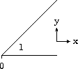
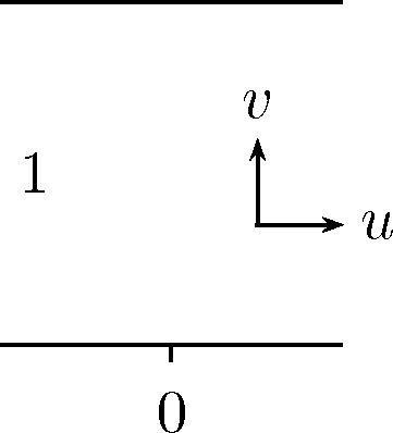
Figure 2. Transformation from wedge to strip.

Let $\mu=\inf\{{\textstyle\frac{1}{\epsilon}},|\lambda|\}$. Furthermore, for $q\in C_{c}^{\infty}(K\backslash(0,0))$, let. $\hat{q}$ be the Laplace transform of $q$ with respect to $u$, where $q(u,v)=q(x,y)$. Suppose that $q$ satisfies (2.24) with $\varphi=0$ (the equation for the linearized pressure). In the transformed variables, the equation for $\hat{q}$ has the form:

$$\lambda^{2}\hat{q}(\lambda,v)+{\textstyle(\frac{1}{\epsilon})^{2}}\hat{q}_{vv}(\lambda,v)\ =\ 0 \text{ in }\mathbb{R}\times(0,1)$$

with boundary conditions $\hat{q}(\lambda,1)=(\lambda+1)\hat{f}(\lambda+1)$ and $\hat{q}_{v}(\lambda,0)=0$. This explicit expression of $\hat{q}$ in Mellin transformed variables motivates the definition of our norms. For any multi-index $\alpha=(\alpha_{1},\alpha_{2})\in\mathbb{R}\times\mathbb{N}_{0}$, we define $|\alpha|=\alpha_{1}+\alpha_{2}$ and $\Lambda^{\alpha}=\lambda^{\alpha_{1}}(\frac{1}{\epsilon}\partial_{\nu})^{\alpha_{2}}$. For any $q_{0}\in C_{c}^{\infty}(K\backslash(0,0))$ and for $\ell\geq 0$, we set

$$\begin{aligned} [q_{0}]_{Y_{\epsilon}^{\ell}}\ &=\ \sum_{|\alpha|=3\ell}\|\sup_{v\in(0,1)}\big{|}e^{\frac{1}{2}\epsilon|\lambda|(1-v)}\Lambda^{\alpha}\mu^{\ell}\widehat{q_{0}}\big{|}\|_{L^{2}({\Re\lambda=3\ell-\frac{3}{2}})}.\end{aligned}$$ (2.45)

For technical reasons that will be explained later, we will use these homogeneous norms in particular for $\ell\in[\frac{2}{3},k]$. Suppose that $f\in X_{\epsilon}^{k}$ and suppose that $q$ is defined as in (2.24) with $\eta=f_{x}$. Since $q=f_{x}$ on $\partial_{1}K$ and since by the definition of $X_{\epsilon}^{k}$ the Taylor polynomial of $f$ of order $n_{k}$ is well-defined, we expect to have control on the supremum norm for derivatives of $q$ up to order $n_{k}-1$, where we recall that $n_{k}=\lceil 3k-\frac{3}{2}\rceil$. Indeed, such an estimate is given in Lemma 5.5.

For $q\in C^{\infty}(K)$, let ${\mathcal{P}}_{q}$ be the Taylor polynomial of $q$ at $(0,0)$ of order $n_{k}-1$ (if $k\in\mathbb{N}$ then $n_{k}-1=3k-2$). Let $\zeta:K\to\mathbb{R}$ be a cut-off function such that $\zeta=\zeta(r)$ with $\zeta=1$ in $[0,\frac{1}{8}]$, $\zeta=0$ outside $[0,\frac{1}{4}]$ and such that $0\leq\zeta\leq 1$. We decompose $q:=q_{0}+q_{1}$ with $q_{1}=\zeta{\mathcal{P}}_{q}$ and define for $k,\ell\in\mathbb{R}$, the norm

$$\|q\|_{Y_{\epsilon}^{k}}\ =\ \|{\mathcal{P}}_{q}\|_{{\mathcal{P}}}+\sup_{\frac{2}{3}\leq\ell\leq k}[q_{0}]_{Y_{\epsilon}^{\ell}}.$$ (2.46)

Here, $\|\cdot\|_{{\mathcal{P}}}$ is any fixed polynomial norm, e.g. the $\ell^{2}$-norm of the coefficients. We do not include the homogeneous norms with $\ell<\frac{2}{3}$ since this would lead to ’negative derivatives’ in the definition of the following norm, cf. (2.49). The spaces $Y_{\epsilon}^{k}$ and ${\stackrel{{\scriptstyle\raisebox{-0.3014pt}[-15.06943pt][-3.01389pt]{\text{\ \tiny oo }}}}{{Y}}}_{\epsilon}^{\raisebox{0.0pt}[0.0pt][0.0pt]{\hskip 0.3014pt$\scriptstyle k$}}$ are defined by completion with respect to functions $C_{c}^{\infty}(K)$ respectively $C_{c}^{\infty}(K\backslash(0,0))$ as before. By the above considerations, the polynomial is uniquely defined and the norm is well–defined. The space $Y_{\epsilon}^{k}({\Omega})$ and its norm are defined by localizing the above definitions (analogously as for the definition of $X_{\epsilon}^{k}({[0,1]})$). The space $TY_{\epsilon}^{k}$ and its norm are defined analogously to $TX_{\epsilon}^{k}$, i.e.

$$\|p\|_{TY_{\epsilon}^{k}({Q})}^{2}=\sum_{1\leq i+j\leq k}\|\partial_{t}^{i}p\|_{L^{2}(Y_{\epsilon}^{j}({Q}))}^{2}.$$ (2.47)

Let us remark that we believe that all homogeneous norms in (6.22) for all real $\ell\in[\frac{2}{3},k]$ can be bounded by the two extremal homogeneous norms ($\ell=\frac{2}{3}$, $\ell=k$). However, the proof of this interpolation inequality does not seem to be straightforward, in particular since the analyticity of the expressions is destroyed by the supremum in $v$ so that the theory of complex interpolation does not seem to apply directly. This is the reason, why we include the information about all the intermediate homogeneous norms into the definition (2.46). This is not necessary in the definition of the norm for the space $X_{\epsilon}^{k}$ in (2.37) since there we have an interpolation result at hand (see Lemma 5.2).

The space $Z_{\epsilon}^{k}$ describes the regularity of functions $g=\Delta_{\epsilon}q$ for $q\in Y_{\epsilon}^{k}$. In view of (2.45), this suggests to consider for real $\ell\in[\frac{2}{3},k]$, the homogeneous norms of type

$$[g_{0}]_{Z_{\epsilon}^{\ell}}\ =\ \sum_{|\alpha|=3\ell-2}\|\sup_{v\in(0,1)}e^{\frac{1}{2}\epsilon|\lambda|(1-v)}\Lambda^{\alpha}\mu^{\ell}|\widehat{g_{0}}|\|_{L^{2}({\Re\lambda=3\ell-\frac{7}{2}})},$$ (2.48)

where the sums are taken over $\alpha=(\alpha_{1},\alpha_{2})\in\mathbb{R}_{+}\times\mathbb{N}_{0}$ using the notation $|\alpha|=\alpha_{1}+\alpha_{2}$. Note that $[g_{0}]_{{\stackrel{{\scriptstyle\raisebox{-0.3014pt}[-15.06943pt][-3.01389pt]{\text{\ \tiny oo }}}}{{Z}}}_{\epsilon}^{\raisebox{0.0pt}[0.0pt][0.0pt]{\hskip 0.21529pt$\scriptstyle\ell$}}}<\infty$ implies $\|g_{0}\|_{L_{y}^{\infty}}=o(x^{(3\ell-7/2)/2})$ for all $g_{0}\in{\stackrel{{\scriptstyle\raisebox{-0.3014pt}[-15.06943pt][-3.01389pt]{\text{\ \tiny oo }}}}{{Z}}}_{\epsilon}^{\raisebox{0.0pt}[0.0pt][0.0pt]{\hskip 0.3014pt$\scriptstyle\ell$}}$. Correspondingly, we say $g\in Z_{\epsilon}^{k}$ if there is a polynomial ${\mathcal{P}}_{g}$ in $x,y$ of order $n_{k}-3$ (if $k\in\mathbb{N}$ then $n_{k}-3=3k-4$) such that $g_{0}:=g-\zeta{\mathcal{P}}_{g}\in{\stackrel{{\scriptstyle\raisebox{-0.3014pt}[-15.06943pt][-3.01389pt]{\text{\ \tiny oo }}}}{{Z}}}_{\epsilon}^{\raisebox{0.0pt}[0.0pt][0.0pt]{\hskip 0.3014pt$\scriptstyle k$}}$ for some radial cut-off $\zeta=\zeta(r)$ with $\zeta=1$ in $[0,1]$ and $\zeta=0$ in $[2,\infty)$. The corresponding norm is given by

$$\|g\|_{Z_{\epsilon}^{k}}\ =\ \|{\mathcal{P}}_{g}\|_{{\mathcal{P}}}+\sup_{\frac{2}{3}\leq\ell\leq k}[g_{0}]_{Z_{\epsilon}^{\ell}}.$$ (2.49)

The spaces ${\stackrel{{\scriptstyle\raisebox{-0.3014pt}[-15.06943pt][-3.01389pt]{\text{\ \tiny oo }}}}{{Z}}}_{\epsilon}^{\raisebox{0.0pt}[0.0pt][0.0pt]{\hskip 0.3014pt$\scriptstyle k$}}$ and $Z_{\epsilon}^{k}$ are defined by completion as before. The corresponding space $Z_{\epsilon}^{k}(\Omega)$ for the droplet case and its norm are defined analogously as before by localizing the above definitions. Note that the minimal value $\ell=\frac{2}{3}$ in (2.49) is chosen such that the exponent $|\alpha|=3\ell-2$ in definition (2.48) stays non-negative.

2.4. Compatibility conditions

Higher regularity for our solution requires compatibility conditions on the initial data (for both Darcy flow and thin-film equation): Indeed, let $f\in TX_{\epsilon}^{k}$ be a solution of (2.25), respectively (2.28). Since $f=0$ at $x=0$, it follows that $\partial_{t}^{k}f_{|x=0}=0$. This translates to a compatibility condition for the initial data. It is obtained by consecutively replacing the time derivatives in $\partial_{t}^{k}f_{|x=0}$ by the spatial operators ${\mathcal{N}}_{\epsilon}$ and $A_{\epsilon}$ using (2.25) resp. (2.28). The corresponding condition needs to be satisfied for the initial data:

$$f_{\rm in}\text{ satisfies compatibility conditions ensuring $\partial_{t}^{l}f_{|x=0}=0$ at $t=0$}$$ (2.50)

for all $0\leq l\leq k$. For example, the condition for $k=1$ corresponds to $N_{\epsilon}(f_{\rm in},f_{\rm in})=A_{\epsilon}f_{\rm in}$. An analogous compatibility condition needs to be satisfied for the linear evolution $f_{t}+A_{\epsilon}f=g$. In this case, we need $f_{\rm in}$ and $g$ to satisfy for all $0\leq l\leq k$

$$f_{\rm in}\text{ and }g\text{ satisfy compatibility conditions ensuring $\partial_{t}^{l}f_{|x=0}=0$ at $t=0$.}$$ (2.51)

3. Statement and discussion of the results

3.1. Statement of results

We have the following main results: We have well-posedness for the Darcy flow with moving contact line. In the regime of lubrication approximation, we have convergence of the solutions towards solutions of the thin-film equation. Furthermore as a consequence, we obtain well-posedness for the thin-film equation.

Theorem 3.1 (Darcy flow).

Let $k\geq 1$ be an integer, $\epsilon\in(0,\frac{\pi}{3(2k+1)})$. Suppose that $f_{\rm in}^{\epsilon}\in X_{\epsilon}^{k+1/2}$ satisfies (2.50) and suppose that $\|f_{\rm in}^{\epsilon}\|_{X_{\epsilon}^{k+1/2}}\leq\alpha_{k}$ for some (small) universal constant $\alpha_{k}$. Then there is a unique global in time solution $f^{\epsilon}\in TX_{\epsilon}^{k}$ of (2.25)_ϵ with initial data $f_{\rm in}^{\epsilon}$. Furthermore,

$$\|f^{\epsilon}\|_{TX_{\epsilon}^{k+1}}+\|\overline{p}^{\epsilon}\|_{TY_{\epsilon}^{k+1}}\ \leq\ C_{k}\|f_{\rm in}^{\epsilon}\|_{X_{\epsilon}^{k+1/2}},$$ (3.1)

where $\overline{p}^{\epsilon}=p^{\epsilon}\circ\Psi^{\epsilon}\in Y_{\epsilon}^{k}$ and $\Psi^{\epsilon}:K\to K^{f^{\epsilon}}$ is the coordinate transform in Lemma 6.5; see also (2.37), (2.45) for the definition of the norms. The constant in (3.1) is universal, in particular it does not depend on $\epsilon$.

The above well-posedness result can also be stated for the Darcy flow in terms of the original variables: Suppose that the assumptions of Theorem 3.1 hold. Then there exists a unique classical solution of (1.2). In particular, if $f_{\rm in}^{\epsilon}$ is sufficiently small then $h_{\rm in}^{\epsilon}$ defined by $\partial_{x}h_{\rm in}^{\epsilon}=1+f_{\rm in}^{\epsilon}$ satisfies $h_{\rm in}^{\epsilon}>0$ for $x>0$.

We also have convergence for solutions of the Darcy flow to solutions of the thin-film equation. Furthermore, as suggested by the asymptotic expansion, in the limit $\epsilon\to 0$, the pressure $p$ is independent of the vertical direction:

Theorem 3.2 (Convergence).

Suppose that the assumptions of Theorem 3.1 are satisfied. Let $f^{\epsilon}$ be the solution of (2.25)_ϵ with initial data $f_{\rm in}^{\epsilon}$ and let $p^{\epsilon}$ be the corresponding pressure. Suppose that $\|f_{\rm in}^{\epsilon}-f_{\rm in}\|_{X_{\epsilon}^{k+1/2}}\to 0$ as $\epsilon\to 0$ for some $f_{\rm in}\in X_{0}^{k+1/2}$. Then there exist $f$, $p$ and a subsequence $\epsilon_{j}\to 0$ such that

$$\|f^{\epsilon_{j}}-f\|_{TX_{\epsilon}^{k}}\to 0\quad\text{and}\quad\|\overline{p}^{\epsilon_{j}}-\overline{p}\|_{TY_{\epsilon}^{k}}\to 0 j\to\infty$$ as , (3.2)

where $\overline{p}^{\epsilon}=p^{\epsilon}\circ\Psi^{\epsilon}\in Y_{\epsilon}^{k}$, with $\Psi^{\epsilon}:K\to K^{f^{\epsilon}}$ defined in (6.34). Furthermore, $f\in{TX}_{0}^{k+1}$ solves (2.28) with initial data $f_{\rm in}$. The limit pressure $p$ does not depend on the vertical direction, i.e. $p=p(t,x)$.

As a consequence of Theorem 3.2, the velocity field $U=(V,W)$ in the limit $\epsilon=0$ is horizontal and does not depend on $y$, i.e. $U=(V(t,x),0)$. By Theorem 3.2 and by Proposition 5.1(2), the solutions converge also in terms of Sobolev norms. We e.g. have

$$\|f^{\epsilon}-f\|_{L_{t}^{2}C_{x}^{3k-1}(\mathbb{R}_{+}^{2})}\to 0,\quad\|\nabla\overline{p}^{\epsilon}-\nabla\overline{p}\|_{L_{t}^{\infty}C_{x}^{3k-2}(\mathbb{R}_{+}\times K)}\to 0 \epsilon\to 0$$ as .

For the case of a droplet as initial data, we have short-time existence:

Theorem 3.3 (Droplet).

Let $k\geq 1$ be an integer, $E=(0,1)$. Suppose that $h_{\rm in}^{\epsilon}\in H^{1}(E)$ with $h_{\rm in}^{\epsilon}>0$ in $(-1,1)$ and with $h_{\rm in}^{\epsilon}=0$, $|h_{\rm in,x}^{\epsilon}|=1$ on $\partial E$. Suppose that $f_{\rm in}^{\epsilon}:=[h_{\rm in}^{\epsilon}-\frac{1}{2}(1-x^{2})]_{x}\in X_{\epsilon}^{k+1/2}({E})$ satisfies the compatibility condition (2.50). Then there is a time $\tau>0$ such that for every $\epsilon\in(0,\frac{\pi}{3(2k+1)})$, there is a unique short–time solution $h^{\epsilon}$ of (1.2) with initial data $h_{\rm in}^{\epsilon}$ (where $h^{\epsilon}$ describes the profile of the propagating liquid). Furthermore, $f^{\epsilon}:=[h^{\epsilon}-\frac{1}{2}(1-x^{2})]_{x}\in TX_{\epsilon}^{k+1}({(0,\tau)\times E})$ satisfies

$$\|f^{\epsilon}\|_{TX_{\epsilon}^{k+1}({(0,\tau)\times E})}\ \leq\ C_{k}\|f^{\epsilon}_{\rm in}\|_{X_{\epsilon}^{k+1/2}({E})}.$$ (3.3)

The solution depends continuously on the initial data. Furthermore $\|f^{\epsilon_{j}}-f\|_{TX_{\epsilon}^{k}}\to 0$ as $j\to\infty$ for a subsequence $\epsilon_{j}\to 0$ and $f$ solves (2.28).

Theorem 3.3 also shows that any solution immediately assumes a regularity of order $\frac{1}{\epsilon}$ where we recall that $\epsilon$ is related to the opening angle. This is the maximal regularity which can be expected in a non-smooth domain with opening angle of order $\epsilon$, see [28].

Corollary 3.4.

Any solution of $f$ as in Theorem 3.3 satisfies $f\in X_{\epsilon}^{K+\frac{1}{2}}({E})$ for any fixed positive time, where $K$ is the largest integer such that $K<\frac{1}{2}(\frac{\pi}{3\epsilon}-1)$.

Indeed, this follows by a bootstrap argument using (3.3): If $f_{\rm in}\in X_{\epsilon}^{k+1/2}({E})$, then we also have $L^{2}(X_{\epsilon}^{k+1}({(0,\tau)\times E}))$ which yields $f\in X_{\epsilon}^{k+1}({E})$ for almost every fixed positive time $t_{0}>0$. Application of Theorem 3.3 then implies $f\in L^{2}(X_{\epsilon}^{k+3/2}({(t_{0},\tau)\times E}))$ for all $t>t_{0}$. Now, for any $\delta$, we may repeatedly apply this argument for time steps of size $\frac{\delta}{K}$ which yields the assertion of Corollary 3.4.

Our analysis also yields the following new existence, uniqueness and regularity result for classical solutions of the thin-film equation:

Theorem 3.5 (Thin-film equation).

Let $k\geq 1$ be integer.

1. There is $\alpha_{k}>0$ such that for any $f_{\rm in}\in X_{0}^{k+1/2}$ with $\|f_{\rm in}\|_{X_{0}^{k+1/2}}\leq\alpha_{k}$ and such that (2.50) is satisfied, there is a unique global in time solution $f\in{TX}_{0}^{k}$ of (2.28) with initial data $f_{\rm in}$. Furthermore, $\|f\|_{{TX}_{0}^{k}}\leq C_{k}\|f_{\rm in}\|_{X_{0}^{k+1/2}}$.

2. Let $f_{\rm in}\in X_{0}^{k+1/2}$ and suppose that the analogous assumptions as in Theorem 3.3 holds. Then there is a short time solution $f\in{TX}_{0}^{k+1}$ of (2.28). Furthermore, $\|f_{\epsilon}\|_{TX_{0}^{k+1}({(0,\tau)\times E})}\leq C_{k}\|f_{\rm in}\|_{X_{0}^{k+1/2}({E})}$.

Note that the existence for weak solutions of the thin-film equation (1.4) in the complete wetting regime (zero contact angle) is well understood, see e.g. [7, 8]; uniqueness of weak solutions is still an open problem. Existence and uniqueness of classical solutions has been shown in [21, 20]. All the above results address the case of complete wetting where the liquid attains a zero contact angle at the triple point. There are only few results for the partial wetting regime where existence (but not uniqueness) of weak solutions is proved [34, 9]. Well-posedness for classical solutions with non-zero contact angle for a related model has been shown in [25]. In this paper, we give the first existence and uniqueness result for (1.4) in the partial wetting regime. We hope that the techniques developed in this paper can also be applied to more complicated systems such as the Stokes flow with various boundary conditions at the liquid-solid interface or for fluid models where the contact angle condition at the triple point is different.

In the following, we do not explicitly write $k$-dependence of constants, i.e. we write $C=C_{k}$.

3.2. Formal lubrication approximation

We formally show how the Darcy flow (2.25) converges to the thin-film equation (2.28). For this, we show convergence of both linear and nonlinear operator in (2.25), i.e. $A_{\epsilon}\to A_{0}$ and $N_{\epsilon}\to N_{0}$ as $\epsilon\to 0$. The argument is based on an asymptotic expansion of the ($\epsilon$-dependent) pressure $p^{\epsilon}$ in $\epsilon y$ (cf. (2.14)):

$$p^{\epsilon}(t,x,y)=p_{0}(t,x)+\epsilon^{2}p_{2}(t,x,{\textstyle\frac{y}{\epsilon}})+{\mathcal{O}}(\epsilon^{4}).$$

Our aim is to solve (2.14) up to first order in $\epsilon$, i.e.

$$\left\{\begin{array}[]{ll}\partial_{x}^{2}p^{\epsilon}+({\textstyle\frac{1}{\epsilon}}\partial_{y})^{2}p^{\epsilon}\ =\ {\mathcal{O}}(\epsilon^{2})&\text{ in }\Omega,\\ p^{\epsilon}_{|\Gamma}\ =\ f_{x},\quad p^{\epsilon}_{y|\Gamma_{0}}\ =\ 0.\end{array}\right.$$ (3.6)

Indeed, the solution of (3.6) has the asymptotic expansion

$$p^{\epsilon}(t,x,y)\ =\ f_{x}-{\textstyle\frac{\epsilon^{2}}{2}}\left(y^{2}-h^{2}\right)f_{xxx}+{\mathcal{O}}(\epsilon^{4}).$$

Inserting this asymptotic expansion into (2.14), we obtain

$$B_{\epsilon}^{\varphi}f_{x}(t,x)\ =\ {\mathcal{B}}_{\epsilon}^{h}f_{x}(t,x)\ \stackrel{{\scriptstyle\eqref{def-bt}}}{{=}}\ -h_{x}f_{xx}-hf_{xxx}+{\mathcal{O}}(\epsilon^{2})\ =\ -(hf_{xx})_{x}+{\mathcal{O}}(\epsilon^{2}).$$ (3.7)

where $h=x+\int_{0}^{x}\varphi$. The asymptotic expression of the linear operator $A_{\epsilon}$ follows as a special case of (3.7) by setting $\varphi=0$ or equivalently $h=x$:

$$A_{\epsilon}f\ \stackrel{{\scriptstyle\eqref{def-A}}}{{=}}\ -(B_{\epsilon}f_{x})_{x}\ \stackrel{{\scriptstyle\eqref{formal-DN}}}{{=}}\ (xf_{xx})_{xx}+{\mathcal{O}}(\epsilon^{2})\ \stackrel{{\scriptstyle\eqref{def-A0}}}{{=}}\ A_{0}f+{\mathcal{O}}(\epsilon^{2}),$$

which implies $A_{\epsilon}\to A_{0}$. The convergence $N_{\epsilon}\to N_{0}$ can be seen similarly: With the notation $\Phi=\int_{0}^{x}\varphi\ dx=h-x$, we have

$$N_{\epsilon}(\varphi,f)\ \ \ \stackrel{{\scriptstyle\eqref{def-N}}}{{=}}\ \varphi_{x}f_{xx|x=0}+(B_{\epsilon}^{\varphi}f_{x})_{x}-(B_{\epsilon}f_{x})_{x}+{\mathcal{O}}(\epsilon^{2})$$

$$\stackrel{{\scriptstyle\eqref{formal-DN}}}{{=}}\ \Phi_{xx}f_{xx|x=0}-(hf_{xx})_{xx}+(xf_{xx})_{xx}+{\mathcal{O}}(\epsilon^{2})$$

$$=\ (\Phi f_{xx|x=0})_{xx}-(\Phi f_{xx})_{xx}+{\mathcal{O}}(\epsilon^{2})\ \ \ \stackrel{{\scriptstyle\eqref{def-A0}}}{{=}}\ N_{0}(\varphi,f)+{\mathcal{O}}(\epsilon^{2})$$

which formally proves the convergence $N_{\epsilon}\to N_{0}$.

4. Proof of Theorems 3.1–3.5

We give the proof of the Theorems 3.1-3.5 already in this section so that the reader may get an overview of the structure of the proof. Some parts of the proof are based on results and estimates which are given in detail in the later part of this work.

4.1. Proof of Theorem 3.1

The proof of Theorem 3.1 proceeds by an application of a contraction principle. It is based on maximal regularity for the linear operator $A_{\epsilon}$ and corresponding bounds for the operator $N_{\epsilon}$. In the following we drop the superscript $\epsilon$ in the notation if the meaning is clear from the context, e.g. $f=f^{\epsilon}$ and correspondingly for the other functions used. The maximal regularity estimate is the following:

Proposition 4.1.

Let $k\geq 1$ be an integer, $\epsilon\in(0,\frac{\pi}{3(2k+1)})$. Suppose that $f_{\rm in}^{\epsilon}\in X_{\epsilon}^{k+1/2}$ and $g\in TX_{\epsilon}^{k-1}$ satisfy (2.51). Then there is a unique global in time solution $f^{\epsilon}\in TX_{\epsilon}^{k}$ of

$$\left\{\begin{aligned} &f_{t}+\ A_{\epsilon}f=g&&\text{for }x\in(0,\infty),\\ &f=0&&\text{for }x=0.\end{aligned}\right.$$ (4.1)

with initial data $f_{\rm in}$. Furthermore, for some uniform constant $C>0$ and all $\tau>0$ and with $Q_{\tau}=(0,\tau)\times(0,\infty)$, we have

$$\|f\|_{TX_{\epsilon}^{k+1}({Q_{\tau}})}\ \leq\ C\ \big{(}\|g\|_{TX_{\epsilon}^{k}({Q_{\tau}})}+\|g\|_{L^{2}(X_{\epsilon}^{0}({Q_{\tau}}))}+\|f_{\rm in}\|_{X_{\epsilon}^{k+1/2}({(0,\infty)})}+\|f\|_{C_{t}^{0}L_{x}^{2}(Q_{\tau}))}\big{)}$$ (4.2)

The estimate on the nonlinear operator is stated in the following proposition:

Proposition 4.2.

Suppose that the assumptions of Theorem 3.1 are satisfied. Suppose for $i=1,2$ that $f_{i}\in TX_{\epsilon}^{k+1}$ with $\|f_{i}\|_{TX_{\epsilon}^{k+1}}$. Then

$$\|N_{\epsilon}(f_{1},f_{1})-N_{\epsilon}(f_{2},f_{2})\|_{TX_{\epsilon}^{k}({Q_{\tau}})}+\|N_{\epsilon}(f_{1},f_{1})-N_{\epsilon}(f_{2},f_{2})\|_{L^{2}(X_{\epsilon}^{0}({Q_{\tau}}))}\$$

$$\leq\ C\|f_{1}-f_{2}\|_{TX_{\epsilon}^{k+1}({Q_{\tau}})}(\|f_{1}\|_{TX_{\epsilon}^{k+1}({Q_{\tau}})}+\|f_{2}\|_{TX_{\epsilon}^{k+1}({Q_{\tau}})}\big{)}.$$ (4.3)

Proposition 4.1 has been derived in [26]. Note the extra term $\|f\|_{C_{t}^{0}L_{x}^{2}(Q_{\tau}))}$ on the right-hand side of (4.2) which is due to the slightly different definition of the norms $\|f\|_{TX_{\epsilon}^{k+1}({Q_{\tau}})}$. This extra term is needed for the nonlinear estimate (4.2). The proof of Proposition 4.2 is shown in Section 6. The estimates in the above two propositions hold for every chosen time interval. The constants do not depend on this interval.

The proof of Theorem 3.1 now follows by application of a contraction argument: For $\delta>0$ to be fixed later, we set

$$E\ :=\ \{f\in TX_{\epsilon}^{k}\ :\ \|f\|_{TX_{\epsilon}^{k}}\ <\ \delta\}.$$ (4.4)

The operator $S_{\epsilon}(f)$ is defined for any $f\in E$ as the solution of (2.25) with fixed initial data $f_{\rm in}$ and right hand side $N_{\epsilon}(f,f)$. Let $f_{1},f_{2}\in E$, with the same initial data and let $f:=f_{1}-f_{2}$. In particular, $S_{\epsilon}(f_{1})-S_{\epsilon}(f_{2})$ solves (2.25) with vanishing initial data and right hand side $N_{\epsilon}(f_{1},f_{1})-N_{\epsilon}(f_{2},f_{2})$. By standard interpolation, we have for any $f\in E$,

$$\|f\|_{C_{t}^{0}L_{x}^{2}(Q_{\tau})}\ \leq\ \|f_{\rm in}\|_{L^{2}({(0,\infty)})}+C\tau\|f\|_{TX_{\epsilon}^{k+1}({Q_{\tau}})}.$$ (4.5)

Hence, there is a small but universal constant $\tau$ such that for $\tau=\tau_{0}$, we can absorb the last term on the right hand side of (4.2) (increasing the constant in the estimate by some universal factor) to get

$$\|f\|_{TX_{\epsilon}^{k+1}({Q_{\tau}})}\ \leq\ C\ \big{(}\|g\|_{(TX_{\epsilon}^{k}\cap L^{2}(X_{\epsilon}^{0})({Q_{\tau}})}+\|f_{\rm in}\|_{X_{\epsilon}^{k+1/2}({(0,\infty)})}\big{)},$$ (4.6)

where we use the notation $\|\cdot\|_{TX_{\epsilon}\cap L^{2}(X_{\epsilon}^{0})}:=\|\cdot\|_{TX_{\epsilon}}+\|\cdot\|_{L^{2}(X_{\epsilon}^{0})}$. By (4.6) and in view of (4.2), we hence get

$$\|S_{\epsilon}(f_{1})-S_{\epsilon}(f_{2})\|_{TX_{\epsilon}^{k+1}}\ \stackrel{{\scriptstyle\eqref{l-2b}}}{{\leq}}\ C\|N_{\epsilon}(f_{1},f_{1})-N_{\epsilon}(f_{2},f_{2})\|_{TX_{\epsilon}^{k}\cap L^{2}(X_{\epsilon}^{0})}$$

$$\stackrel{{\scriptstyle\eqref{nl-1}}}{{\leq}}\ C\|f_{1}-f_{2}\|_{TX_{\epsilon}^{k+1}}\ \big{(}\|f_{1}\|_{TX_{\epsilon}^{k+1}}+\|f_{2}\|_{TX_{\epsilon}^{k+1}}\big{)}$$

$$\leq\ C\delta\|f_{1}-f_{2}\|_{TX_{\epsilon}^{k+1}}.$$

Hence, $S_{\epsilon}$ is a contraction if $\delta>0$ and $\tau$ are chosen sufficiently small. Similarly, by (4.6), (4.2) and since $N_{\epsilon}(0)=0$, we get

$$\|S_{\epsilon}(f)\|_{TX_{\epsilon}^{k+1}}\ \stackrel{{\scriptstyle\eqref{l-2b}}}{{\leq}}\ C\|N_{\epsilon}(f)\|_{TX_{\epsilon}^{k}\cap L^{2}(X_{\epsilon}^{0})}+C\|f_{\rm in}\|_{X_{\epsilon}^{k+1/2}}\ \stackrel{{\scriptstyle\eqref{nl-1}}}{{\leq}}\ C\alpha+C\delta^{2}$$

and hence $S_{\epsilon}(E)\subseteq E$ for $\delta$ and $\alpha=\alpha(\delta)$ sufficiently small. Therefore, application of Banach’s Fix-point Theorem yields existence and uniqueness of a solution of (2.25) on the time interval $(0,1)$. In order to recover long-time existence, we use dissipation of energy (1.5). Indeed, by (1.5), we have

$$\|f\|_{C_{t}^{0}L_{x}^{2}(Q_{\tau})}\ \leq\ C\|f_{\rm in}\|_{L^{2}({(0,\infty)})}\ \leq\ C\|f_{\rm in}\|_{X_{\epsilon}^{k+1/2}}.$$ (4.7)

Using this estimate instead of (4.5), we get estimates that are independent of the time interval. This shows long-time existence and also the estimate of $f$ in (3.1). In order to conclude the proof of Theorem 3.1, it remains to prove the uniform bound (3.1) on $p$. This estimate follows from the estimate in Proposition 6.7.

4.2. Proof of Theorem 3.2

By Theorem 3.1, we have the uniform bound $\|f^{\epsilon}\|_{TX_{\epsilon}^{k+1}}\leq C\alpha$ for all $\epsilon>0$. We use the optimal decomposition into high and low frequencies $f^{\epsilon}=f^{\epsilon}_{+}+f^{\epsilon}_{-}$ from (5.6). By (5.6), this decomposition commutes with the time derivative. We have uniform bounds on the norms $\|x^{2j+1}\partial_{t}^{i}\partial_{x}^{4j+1}f^{\epsilon}_{+}\|_{L^{2}({(0,\infty)^{2}})}$ and $\|x\partial_{t}^{i}\partial_{x}^{3j+1}f^{\epsilon}_{-}\|_{L^{2}({(0,\infty)^{2}})}$ for all $i$, $j$ with $i+j\leq k+1$. Standard compactness applied to both $f^{\epsilon}_{\pm}$ then show that in particular there is $f=f^{0}_{+}+f^{0}_{-}\in{TX}_{0}^{k}$ and a subsequence $\epsilon_{j}\to 0$ such that

$$\|f^{\epsilon_{j}}-f\|_{TX_{\epsilon_{j}}^{k}}\to 0 j\to\infty$$ as . (4.8)

Now, let $p^{\epsilon_{i}}$, $p^{\epsilon_{j}}$ be the pressure related to $f^{\epsilon_{i}}$ and $f^{\epsilon_{j}}$. By (6.7), we then have

$$\|p^{\epsilon_{i}}-p^{\epsilon_{j}}\|_{TY_{\epsilon_{j}}^{k}}\ \leq\ C\|f^{\epsilon_{i}}-f^{\epsilon_{j}}\|_{TX_{\epsilon_{j}}^{k}}(\|f^{\epsilon_{i}}\|_{TX_{\epsilon_{j}}^{k}}+\|f^{\epsilon_{j}}\|_{TX_{\epsilon_{j}}^{k}})\ \stackrel{{\scriptstyle\eqref{conv-1}}}{{\leq}}\ C\alpha\|f^{\epsilon_{i}}-f^{\epsilon_{j}}\|_{TX_{\epsilon_{j}}^{k}}\to 0$$

as $i,j\to\infty$, $j\leq i$. This shows that $p^{\epsilon_{j}}$ converges in $TY_{\epsilon}^{k}$ thus concluding the proof of (3.2).

It remains to show that $f$ solves the thin-film equation (2.28). By the above uniform bounds, by (5.2) and by (5.11), we have $f^{\epsilon}\to f$ in $L^{2}(H^{4})$, $f^{\epsilon}_{t}\to f_{t}$ in $L^{2}(L^{2})$ and $p^{\epsilon}\to p$ in $L^{2}(H^{1})$ with $\|p_{y}^{\epsilon}\|_{L^{2}(L^{2})}\leq C\epsilon\to 0$. The boundary condition $p^{\epsilon}=h_{xx}(1+\epsilon^{2}h_{x}^{2})^{-\frac{3}{2}}$ hence implies that in the limit $\epsilon=0$, we get $p=h_{xx}$. We will show that in the limit $\epsilon=0$, $h$ is a solution of the thin-film equation, where we recall that $f^{\epsilon}=h^{\epsilon}_{x}-1$. In particular, $h^{\epsilon}\to h$ in $L^{2}(H^{4})$ and $h_{t}^{\epsilon}\to h_{t}$ in $L^{2}(L^{2})$. Correspondingly, we also have convergence of the velocity $u^{\epsilon}=(v^{\epsilon},w^{\epsilon})=\nabla_{\epsilon}p^{\epsilon}\to u=(v,w)=(p_{x},0)$ in $L^{2}(L^{2})$. The transition to the limit now can be conveniently done in terms of the continuity equation: By conservation of mass for (2.25), we have

$$h^{\epsilon}_{t}+\Big{(}\int_{0}^{h^{\epsilon}(t,x)}v^{\epsilon}\ d\tilde{x}\Big{)}_{x}\ =\ 0.$$ (4.9)

In the limit $\epsilon\to 0$ and in view of the above discussion, (4.9) turns into

$$h_{t}+\Big{(}\int_{0}^{h(t,x)}v\ d\tilde{x}\Big{)}_{x}\ =\ h_{t}+(hp_{x})_{x}\ =\ h_{t}+(hh_{xxx})_{x}\ =\ 0.$$ (4.10)

4.3. Proof of Theorem 3.3

We prove this theorem by an application of the Inverse Function Theorem. For this, we linearize ${\mathcal{L}}_{\epsilon}$ at an ‘approximate solution’ $w$, constructed with the help of an extension lemma. We then show boundedness and differentiability for ${\mathcal{L}}_{\epsilon}$ and invertibility and maximal regularity for its linearization $\delta{\mathcal{L}}_{\epsilon}^{w}$ at $w$. We keep the details brief and refer to similar arguments in [14, 20, 3].

We define the ‘spatial part’ ${\mathcal{A}}_{\epsilon}$ of the operator ${\mathcal{L}}_{\epsilon}$ by ${\mathcal{L}}_{\epsilon}f=Df_{t}+{\mathcal{A}}_{\epsilon}f$, i.e.

$${\mathcal{A}}_{\epsilon}f\ :=\ D_{t}f-\partial_{x}\Big{[}\big{(}(1-x)\dot{s}_{-}+x\dot{s}_{+}\big{)}(f+(x(1-x))_{x})+B_{\epsilon}^{f}\Big{(}\frac{f_{x}-2}{(1+\epsilon^{2}(f+(x(1-x))_{x})^{2})^{\frac{3}{2}}}\Big{)}\Big{]},$$

see (2.15). We will use the following extension Lemma

Lemma 4.3 (Extension Lemma).

Let $k\in\mathbb{N}$ with $k\geq 1$. For any $f_{\rm in}\in X_{\epsilon}^{k+1/2}({E})$, $g_{\rm in}\in X_{\epsilon}^{k-1/2}({E})$ there exists $w\in TX_{\epsilon}^{k+1}({[0,\infty)\times E})$ such that $w_{|t=0}=f_{\rm in}$, $w_{t{|t=0}}=g_{\rm in}$ and

$$\|w\|_{TX_{\epsilon}^{k+1}({[0,\infty)\times E})}\ \leq\ C\big{(}\|f_{\rm in}\|_{X_{\epsilon}^{k+1/2}({E})}+\|g_{\rm in}\|_{X_{\epsilon}^{k-1/2}({E})}\big{)}.$$ (4.11)

The extension can be constructed by gluing together solutions of the linear equation given by Proposition 4.1. The methods used in [20] can also be used for our equation so that we will not present the argument here. For $f_{\rm in}\in X_{\epsilon}^{k}$, let $g_{\rm in}=-{\mathcal{A}}_{\epsilon}f_{\rm in}$ and we choose $w\in TX_{\epsilon}^{k+1}({[0,\infty)\times E})$ as in Lemma 4.3. In particular,

$${\mathcal{L}}_{\epsilon}w|_{t=0}\ =\ D\partial_{t}w|_{t=0}+{\mathcal{A}}_{\epsilon}f_{\rm in}\ \stackrel{{\scriptstyle D|_{t=0}=1}}{{=}}\ g_{\rm in}-g_{\rm in}\ =\ 0$$ (4.12)

and $w$ may in this sense be called an approximate solution. Let $\delta\mathcal{L}_{\epsilon}^{w}$ be the linearization of $\mathcal{L}_{\epsilon}$ around $w$. We have boundedness and differentiability of ${\mathcal{L}}_{\epsilon}$ and boundedness of $(\delta{\mathcal{M}}(w))^{-1}$ for $\tau$ small enough:

Proposition 4.4.

Let $k\geq 1$, $k\in\mathbb{N}$ and suppose that $f_{\rm in}\in X_{\epsilon}^{k+1/2}({E})$ with $\int f_{\rm in}dx=0$ and $g\in TX_{\epsilon}^{k}({Q_{\tau}})$ satisfy (2.51). Let $w\in X_{\epsilon}^{k+1}({[0,\infty)\times E})$ be defined as in Lemma 4.3 with $g_{\rm in}:=g_{|t=0}$. Then for sufficiently small $\tau>0$ and with the notation $Q_{\tau}=(0,\tau)\times E$, there exists a unique $f\in TX_{\epsilon}^{k+1}({Q_{\tau}})$, solution of $\delta\mathcal{L}_{\epsilon}(w)f\ =\ g$ in $Q_{\tau}$ with $f=0$ on $(0,\tau)\times\partial E$ and with initial data $f=f_{\rm in}$. Furthermore,

$$\|f\|_{TX_{\epsilon}^{k+1}({Q_{\tau}})}\ \leq\ C\big{(}\|g\|_{TX_{\epsilon}^{k}({Q_{\tau}})}+\|f_{\rm in}\|_{X_{\epsilon}^{k+1/2}({E})}\big{)}.$$ (4.13)

Note that the condition $\int_{0}^{1}f(x)dx=0$ is preserved by the flow generated by $\delta\mathcal{L}_{\epsilon}(w)f$ . We also have differentiability of ${\mathcal{L}}_{\epsilon}$ in a neighborhood of $w$:

Proposition 4.5.

Suppose that $f_{\rm in}\in X_{\epsilon}^{k+1/2}({E})$ satisfies (2.50) and $\int_{E}f_{\rm in}dx=0$ and let $w$ be defined as in Lemma 4.3 with $g_{\rm in}=-{\mathcal{A}}_{\epsilon}f_{\rm in}$. Then for sufficiently small $\tau>0$ there is $\alpha>0$ such that ${\mathcal{M}}_{\epsilon}:TX_{\epsilon}^{k+1}({Q_{\tau}})\to X_{\epsilon}^{k+1/2}({E})\times TX_{\epsilon}^{k}({Q_{\tau}})$ is bounded and continuously differentiable in the $\alpha$-neighborhood of $w$ in $TX_{\epsilon}^{k+1}({Q_{\tau}})$.

The proof of the above two propositions is given in Section 7. Using the above two propositions, the proof of Theorem 3.3 follows by application of the inverse function theorem: We claim that the operator

$${\mathcal{M}}_{\epsilon}:TX_{\epsilon}^{k+1}({Q_{\tau}})\to TX_{\epsilon}^{k+1/2}({E})\times TX_{\epsilon}^{k}({Q_{\tau}}) f\ \mapsto\ {\mathcal{M}}_{\epsilon}(f)\ :=\ (f_{|t=0},\mathcal{L}_{\epsilon}f)$$ with

is bounded, continuously differentiable near $w$ and $\delta{\mathcal{M}}_{\epsilon}(w)$ is invertible with bounded inverse for $\tau$ small enough. We define $v:={\mathcal{L}}_{\epsilon}(w)$. By the inverse mapping theorem there is a neighborhood of $w$ and a neighborhood of $(f_{\rm in},v)$ where $\mathcal{M}_{\epsilon}$ is a diffeomorphism. By (4.12) we have $v_{|t=0}=0$. Since $C_{c}^{\infty}(\overline{Q}_{\tau})$ is dense in $TX_{\epsilon}^{k}({Q_{\tau}})$, it follows that $\|v\|_{TX_{\epsilon}^{k}({Q_{\tau}})}\to 0$ for $\tau\to 0$. Hence, there is $\tilde{\tau}\in(0,\tau)$ and a function $\tilde{v}\in Y_{\tau}$ with $\tilde{v}=0$ for $t\in(0,\tilde{\tau})$ and such that $(0,\tilde{v})$ is sufficiently near $(0,v)$. Hence, there is $f\in X_{\tau}$ with $\mathcal{M}_{\epsilon}(f)=(0,\tilde{v})$. The function $f$ is a solution of ${\mathcal{L}}_{\epsilon}f=0$ and hence $h(x)=x(1-x)+\int_{0}^{x}f(x^{\prime})dx^{\prime}$ is a solution of (2.17) for $t\in(0,\tilde{\tau})$, thus concluding the proof of Theorem 3.3.

4.4. Proof of Theorem 3.5

By Theorem 3.2, we have existence and regularity of solutions of (2.17) for initial data which are close to the infinite wedge. In order to show Theorem 3.5(1) it hence remains to prove uniqueness of solutions. For this, it is enough to show that the corresponding results in Propositions 4.1 and 4.2 also hold in the case $\epsilon=0$ and for the operators $A_{0}$ and $N_{0}$. The estimate for existence, regularity and uniqueness in the case of half-space then follows by the same fix-point argument as for Theorem 3.1.

The $\epsilon=0$ version of Proposition 4.1 has been proved in [26]. The $\epsilon=0$-version of Proposition 4.2 can be obtained by analogous estimates as the one’s applied in the proof of Proposition 8.1 in [21]. In fact, the estimate is easier in our situation since we only need for an estimate in weighted Sobolev spaces, not the interpolation spaces used in [21]. Finally, we note that the local result in Theorem 3.5 can be obtained by standard localization techniques. The argument can be performed analogously as our localization argument in Section 7; the argument is easier since for $\epsilon=0$, the norms $\|\cdot\|_{X_{\epsilon}^{k}}$ are local. We also refer to a similar localization argument in [20], performed for a thin-film equation in a Hölder space setting.

5. Estimates in weighted spaces

We recall some basic properties of the space $X_{\epsilon}^{k}$ (see Proposition 2.3 of [26]):

Proposition 5.1.

Let $k\in\mathbb{R}$ with $k\geq 0$ and let $f\in X_{\epsilon}^{k}$.

1. For $0\leq\epsilon\leq\epsilon^{\prime}$, we have $X_{\epsilon}^{k}\subseteq X_{\epsilon^{\prime}}^{k}$ and for all $f\in X_{\epsilon}^{k}$

   $$[f]_{X_{\epsilon^{\prime}}^{k}}\ \leq\ [f]_{X_{\epsilon}^{k}}.$$ (5.1)

2. For any $\ell_{1},\ell_{1}\in\mathbb{N}_{0}$ with $0\leq\ell_{1}\leq 3k$ and $0\leq\ell_{2}<3k-\frac{1}{2}$, we have

   $$\begin{aligned} \|\partial_{x}^{\ell_{1}}f\|_{L^{2}}+\|\partial_{x}^{\ell_{2}}f\|_{L^{\infty}}\ \leq\ C\|f\|_{X_{\epsilon}^{k}}.\end{aligned}$$ (5.2)

3. If $f\in X_{\epsilon}^{k}$, then $\partial_{x}f\in X_{\epsilon}^{k-1/2}$, $\partial_{x}^{2}f$, $\partial_{x}^{3}f\in X_{\epsilon}^{k-1}$ and

   $$\|f_{x}\|_{X_{\epsilon}^{k-1/2}}+\|f_{xx}\|_{X_{\epsilon}^{k-1}}+\|f_{xxx}\|_{X_{\epsilon}^{k-1}}\ \leq\ C\|f\|_{X_{\epsilon}^{k}}.$$ (5.3)

The norm $\|\cdot\|_{X_{\epsilon}^{k}}$ controls a scale of weighted Sobolev spaces of fractional order:

Lemma 5.2.

Let $\epsilon\in[0,1)$, $k\geq 0$ and $f_{0}\in{\stackrel{{\scriptstyle\raisebox{-0.3014pt}[-15.06943pt][-3.01389pt]{\text{\ \tiny oo }}}}{{X}}}_{\epsilon}^{\raisebox{0.0pt}[0.0pt][0.0pt]{\hskip 0.3014pt$\scriptstyle k$}}$. Then for every $0\leq\ell\leq k$, we have

$$\|\lambda^{3\ell+1}\mu^{\ell}\widehat{f_{0}}\|_{L^{2}({\Re\lambda=3\ell-\frac{1}{2}})}+\|\widehat{f_{0}}\|_{L^{2}({\Re\lambda=3\ell-\frac{1}{2}})}\ \leq\ C\|f_{0}\|_{X_{\epsilon}^{\ell}}.$$ (5.4)

We have the following characterization of the homogeneous norms:

Lemma 5.3.

Let $k\in\mathbb{N}_{0}$, $\epsilon\in[0,\frac{\pi}{3(2k+1)})$. Then for $f_{0}\in{\stackrel{{\scriptstyle\raisebox{-0.3014pt}[-15.06943pt][-3.01389pt]{\text{\ \tiny oo }}}}{{X}}}_{\epsilon}^{\raisebox{0.0pt}[0.0pt][0.0pt]{\hskip 0.3014pt$\scriptstyle k$}}$ we have

$$c[f_{0}]_{X_{\epsilon}^{k}}\leq\ \inf_{f_{0}=f_{+}+f_{-}}(\|\lambda^{4k+1}\widehat{f_{+}}\|_{L^{2}({\Re\lambda=\beta_{k}})}+\|({\textstyle\frac{1}{\epsilon}})^{k}\lambda^{3k+1}\widehat{f_{-}}\|_{L^{2}({\Re\lambda=\beta_{k}})}\big{)}\ \leq C[f_{0}]_{X_{\epsilon}^{k}},$$ (5.5)

where $\beta_{k}=3k-\frac{1}{2}$. Up to multiplication by a constant that only depends on $k$, for any even integer $M$ with $M\geq k$ the minimum in the right hand side of (5.5) is achieved by

$$\widehat{f_{+}}(\lambda)\ =\ (1-(i\tan)^{M}(\epsilon\lambda))\hat{f}_{0}(\lambda), \widehat{f_{-}}(\lambda)\ =\ (i\tan)^{M}(\epsilon\lambda)\hat{f}_{0}(\lambda).$$ and (5.6)

Furthermore,

$$|\lambda|^{k}|\widehat{f_{+}}(\lambda)|\ \leq\ C\mu^{k}|\hat{f}(\lambda)|, ({\textstyle\frac{1}{\epsilon}})^{k}|\widehat{f_{-}}(\lambda)|\ \leq\ C\mu^{k}|\hat{f}(\lambda)|.$$ (5.7)

The proof of Proposition 5.1, Lemma 5.3 and Lemma 5.2 is given in [26].

The space $X_{\epsilon}^{k}$ is an algebra as is proved below. Note that there is a proof for the algebra property in [26]). The advantage of the result below is that it also applies to the case $k=1$, also the proof is simpler than in [26]:

Lemma 5.4.

For $k\in\mathbb{N}$ with $k\geq 1$ and $f,g\in X_{\epsilon}^{k}$, we have $fg\in X_{\epsilon}^{k}$ and

$$\|fg\|_{X_{\epsilon}^{k}}\ \leq\ C\|f\|_{X_{\epsilon}^{k}}\|g\|_{X_{\epsilon}^{k}}.$$ (5.8)

Proof.

We decompose $f=f_{1}+f_{0}$ and $g=g_{1}+g_{0}$ where $f_{1}={\mathcal{P}}_{f}\zeta$, $g_{1}={\mathcal{P}}_{g}\zeta$ and where ${\mathcal{P}}_{f}$, ${\mathcal{P}}_{g}$ are the Taylor polynomials of $f$, $g$ of order $3k-1$. The cut-off function $\zeta$ is defined as for the definition of (2.37). In particular, $f_{0},g_{0}\in X_{\epsilon}^{k}$. We need to estimate the products $f_{1}g_{1}$, $f_{0}g_{1}$, $f_{1}g_{0}$ and $f_{0}g_{0}$. Clearly $\|f_{1}g_{1}\|_{X_{\epsilon}^{k}}\leq C\|f_{1}\|_{X_{\epsilon}^{k}}\|g_{1}\|_{X_{\epsilon}^{k}}$. As in (5.6), we decompose $f_{0}=f_{+}+f_{-}$ and $g_{0}=g_{+}+g_{-}$. The mixed term $f_{1}g_{0}$ is estimated as follows

$$[f_{1}g_{0}]_{X_{\epsilon}^{k}}\ \leq\ C\|x^{k+1}\partial^{4k}(f_{1}g_{+})\|_{L^{2}({(0,\infty)})}+\|{\textstyle(\frac{1}{\epsilon})}^{k}x\partial^{3k}(f_{1}g_{-})\|_{L^{2}({(0,\infty)})}$$

$$\leq\ C\|f\|_{X_{\epsilon}^{k}}\big{(}\|x^{k+1}\partial^{4k}g_{+}\|_{L^{2}}+\|x\partial^{3k}g_{-}\|_{L^{2}}\big{)}\ \leq\ C\|f\|_{X_{\epsilon}^{k}}\|g\|_{X_{\epsilon}^{k}},$$

The second estimate follows since all derivatives of $f_{1}$ are supported in $(\frac{1}{8},\frac{1}{4})$ and since $x$ is of order $1$ in this interval. The estimate of $f_{0}g_{1}$ proceeds analogously.

It remains to show the estimate for the product $f_{0}g_{0}=f_{+}g_{+}+f_{+}g_{-}+f_{-}g_{+}+f_{-}g_{-}$. In particular, since $f_{0},g_{0}\in{\stackrel{{\scriptstyle\raisebox{-0.3014pt}[-15.06943pt][-3.01389pt]{\text{\ \tiny oo }}}}{{X}}}_{\epsilon}^{\raisebox{0.0pt}[0.0pt][0.0pt]{\hskip 0.3014pt$\scriptstyle k$}}$, we have $|f_{0}|,|g_{0}|\leq Cx^{3k-1}$ for small $x$. It follows that $|f_{0}g_{0}|\leq Cx^{6k-2}\leq Cx^{3k-2}$ (since $k\geq 1$), in particular $f_{0}g_{0}\in{\stackrel{{\scriptstyle\raisebox{-0.3014pt}[-15.06943pt][-3.01389pt]{\text{\ \tiny oo }}}}{{X}}}_{\epsilon}^{\raisebox{0.0pt}[0.0pt][0.0pt]{\hskip 0.3014pt$\scriptstyle k$}}$. We show the estimate for the term high-high-frequency product $f_{-}g_{-}$. Recall that the Mellin transform for the product of functions can be expressed as a convolution for the Mellin transformed functions. Hence,

$$[f_{-}g_{-}]_{X_{\epsilon}^{k}}\ \stackrel{{\scriptstyle\eqref{norm-lambda}}}{{=}}\ \|\lambda^{3k+1}\mu^{k}\int_{\Re\eta=\alpha}\hat{f}_{-}(\lambda-\eta)\hat{g}_{-}(\eta)\ d\Im(\eta)\|_{L^{2}({\Re\lambda=3k-\frac{1}{2}})},$$ (5.9)

where $\mu=\min\{{\textstyle\frac{1}{\epsilon}},|\lambda|\}$ and where $\alpha\in\mathbb{R}$ is chosen such that the product $\hat{f}_{-}(\lambda-\cdot)\hat{g}_{-}(\cdot)$ is absolutely integrable on the line $\Re\eta=\alpha$. Since $\mu\leq{\textstyle\frac{1}{\epsilon}}$, the right-hand side of (5.9) can be estimated by replacing $\mu^{k}$ by $({\textstyle\frac{1}{\epsilon}})^{k}$. Using the binomial formula $\lambda^{3k+1}=\sum_{i}c_{ki}\eta^{i}(\lambda-\eta)^{3k+1-i}$, (5.9) is bounded by above by the sum of the terms

$$I_{k,i}(f_{-},g_{-})=\int_{\Re\lambda=3k-\frac{1}{2}}\left|\int_{\Re\eta=\alpha}({\textstyle\frac{1}{\epsilon}})^{k}(\lambda-\eta)^{3k+1-i}\widehat{f_{-}}(\lambda-\eta)\eta^{i}\widehat{g_{-}}(\eta)\ d\Im(\eta)\right|^{2}\ d\Im(\lambda),$$

where $0\leq i\leq 3k+1$. By symmetry, it is enough to estimate the terms with $i\leq\frac{3}{2}k+\frac{1}{2}$. Note that the integrand of the inner integral above is analytic as a function of $\eta$. In particular, the value of the integral does not depend on $\alpha$. This argument works since we have avoided to replace $\lambda$ by $|\lambda|$ in our proof. By Young’s inequality for convolutions and by the Cauchy-Schwarz inequality, we have

$$\|\hat{F}*\hat{G}\|_{L^{2}({\Re\lambda=\beta})}\ \leq\ C_{\delta}\|(1+|\lambda|^{\delta})\hat{F}\|_{L^{2}({\Re\lambda=\beta_{1}})}\|\hat{G}\|_{L^{2}({\Re\lambda=\beta_{2}})},$$ (5.10)

which holds for all $\delta>\frac{1}{2}$. With the choice $\alpha=i$ and $\delta=1$, we get

$$I_{k,i}(f_{-},g_{-})\ \stackrel{{\scriptstyle\eqref{often-1}}}{{\leq}}\ C\|({\textstyle\frac{1}{\epsilon}})^{k-\frac{i}{3}}|\lambda|^{3k+1-i}\widehat{f_{-}}\|_{L^{2}({\Re\lambda=3k-i-\frac{1}{2}})}\|({\textstyle\frac{1}{\epsilon}})^{\frac{i}{3}}(1+|\lambda|^{i+1})\widehat{g_{-}}\|_{L^{2}({\Re\lambda=i})}$$

$$\stackrel{{\scriptstyle\eqref{est-fpm}}}{{\leq}}\ C\|\mu^{k-\frac{i}{3}}|\lambda|^{3k-i+1}\widehat{f_{0}}\|_{L^{2}({\Re\lambda=3k-i-\frac{1}{2}})}\|\mu^{\frac{i}{3}}(1+|\lambda|^{i+1})\widehat{g_{0}}\|_{L^{2}({\Re\lambda=i})}$$

$$\stackrel{{\scriptstyle\eqref{est-real}}}{{\leq}}\ C\|f\|_{X_{\epsilon}^{k}}\|g\|_{X_{\epsilon}^{k}}.$$

The last estimate follows from (5.4) using $0\leq i\leq\frac{3}{2}k+\frac{1}{2}$ (and since $k\geq 1$). The estimate of the terms $f_{+}g_{-}$, $f_{-}g_{+}$ and $f_{+}g_{+}$ proceeds analogously (see also the related proof in [26]). This concludes the proof of the Lemma. ∎

Also the space $Y_{\epsilon}^{k}$ is embedded into classical Sobolev spaces: For any multi-index $\alpha\in\mathbb{R}_{\geq 0}\times\mathbb{N}_{0}$, we set $|\alpha|=\alpha_{1}+\alpha_{2}$. For $\alpha\in\mathbb{N}^{2}$ we also use the notation $D_{\epsilon}^{\alpha}=\partial_{x}^{\alpha_{1}}(\frac{1}{\epsilon}\partial_{y})^{\alpha_{2}}$.

Lemma 5.5.

Let $k\in\mathbb{R}$ with $k\geq 1$, $\epsilon\in(0,1)$ and let $q\in Y_{\epsilon}^{k}$. Then for all $\ell_{1}$, $\ell_{2}\in\mathbb{N}_{0}$ with $\ell_{1}<3k-1$ and $\ell_{2}\leq 3k-\frac{3}{2}$ (or equivalently $\ell_{2}\leq n_{k}-1$), we have

$$\sum_{0\leq|\alpha|\leq\ell_{1}}\|D_{\epsilon}^{\alpha}q\|_{L_{y}^{\infty}L_{x}^{2}(K)}+\sum_{0\leq|\alpha|\leq\ell_{2}}\sup_{y\in(0,x)}\|D_{\epsilon}^{\alpha}q\|_{L^{\infty}(K)}\ \leq\ C\|q\|_{Y_{\epsilon}^{k}},$$ (5.11)

where the sums are taken over multiindices $\alpha\in\mathbb{Z}^{2}$.

Proof of Lemma 5.5.

Let $q=q_{0}+q_{1}$ with $q_{0}\in{\stackrel{{\scriptstyle\raisebox{-0.3014pt}[-15.06943pt][-3.01389pt]{\text{\ \tiny oo }}}}{{Y}}}_{\epsilon}^{\raisebox{0.0pt}[0.0pt][0.0pt]{\hskip 0.3014pt$\scriptstyle k$}}$ be the decomposition as in (2.45). By definition, $q_{1}$ solves (5.11). It suffices to show the estimate (5.11) for $q_{0}\in{\stackrel{{\scriptstyle\raisebox{-0.3014pt}[-15.06943pt][-3.01389pt]{\text{\ \tiny oo }}}}{{Y}}}_{\epsilon}^{\raisebox{0.0pt}[0.0pt][0.0pt]{\hskip 0.3014pt$\scriptstyle k$}}$. By application of Plancherel’s identity, we have

$$\sum_{|\alpha|=3\ell-1}\sup_{y\in(0,x)}\|D_{\epsilon}^{\alpha}q_{0}\|_{L^{2}({(0,\infty)})}\ \leq\ C\sum_{|\alpha|=3\ell-1}\sup_{v\in(0,1)}\|\partial_{u}^{\alpha_{1}}{(\textstyle\frac{1}{\epsilon}\partial_{v})}^{\alpha_{2}}q_{0}\|_{L^{2}({(0,\infty)})}$$

$$\stackrel{{\scriptstyle\eqref{Y-hom}}}{{\leq}}\ C\sum_{|\alpha|=3\ell-1}\sup_{v\in(0,1)}\|\Lambda^{\alpha}\widehat{q_{0}}\|_{L^{2}({\Re\lambda=3\ell-\frac{3}{2}})}\ \leq\ C[q_{0}]_{Y_{\epsilon}^{k}}.$$

This yields the $L^{2}$ estimate, the supremum estimate follows by standard interpolation. ∎

For any $f\in TX_{\epsilon}^{k+1}$, its trace at $t=0$ is well-defined in $X_{\epsilon}^{k+1/2}$:

Lemma 5.6.

Let $k,\gamma\in\mathbb{N}_{0}$. For $f\in TX_{\epsilon}^{k+1}$ we have

$$\|\partial_{t}^{i}f\|_{C^{0}(X_{\epsilon}^{k+1/2})}\ \leq\ C\|\partial_{t}^{i+1}f\|_{L^{2}(X_{\epsilon}^{k})}+C\|\partial_{t}^{i}f\|_{L^{2}(X_{\epsilon}^{k+1})}.$$ (5.12)

Proof.

It suffices to give the proof for $i=0$ (for $i>0$ consider $F=\partial_{t}^{i}f$ instead). By an approximation argument it is enough to consider $f\in C_{c}^{\infty}([0,\infty)^{2})$ . We decompose $f=f_{0}+f_{1}$ where $f_{1}={\mathcal{P}}_{f}\zeta$ and where ${\mathcal{P}}_{f}$ is the Taylor polynomial of order $n_{k+1/2}=3k$ of $f$ at $x=0$; in particular, $f_{0}\in{\stackrel{{\scriptstyle\raisebox{-0.3014pt}[-15.06943pt][-3.01389pt]{\text{\ \tiny oo }}}}{{X}}}_{\epsilon}^{\raisebox{0.0pt}[0.0pt][0.0pt]{\hskip 0.3014pt$\scriptstyle k+1/2$}}$. In order to avoid fractional derivatives which appear in the definition of the norm for $X_{\epsilon}^{k+1/2}$, we use the equivalence $c[f_{0}]_{X_{\epsilon}^{k+1/2}}\leq\langle Af_{0},f_{0}\rangle_{X_{\epsilon}^{k}}\leq C[f_{0}]_{X_{\epsilon}^{k+1/2}}$ which holds for all $f_{0}\in{\stackrel{{\scriptstyle\raisebox{-0.3014pt}[-15.06943pt][-3.01389pt]{\text{\ \tiny oo }}}}{{X}}}_{\epsilon}^{\raisebox{0.0pt}[0.0pt][0.0pt]{\hskip 0.3014pt$\scriptstyle k+1/2$}}$. A proof of this equivalence is given for $k=0$ in [26, Lemma 4.6], the argument used there also applies for general $k\in\mathbb{N}$. The estimate of the homogeneous part is then easy: For $f,g\in{\stackrel{{\scriptstyle\raisebox{-0.3014pt}[-15.06943pt][-3.01389pt]{\text{\ \tiny oo }}}}{{X}}}_{\epsilon}^{\raisebox{0.0pt}[0.0pt][0.0pt]{\hskip 0.3014pt$\scriptstyle k+1/2$}}\cap X_{\epsilon}^{k+1}$, we have $\langle A_{\epsilon}f_{0},g_{0}\rangle_{X_{\epsilon}^{k}}=\langle f_{0},A_{\epsilon}g_{0}\rangle_{X_{\epsilon}^{k}}$. Hence, integrating in time from infinity (where $f=0$), we obtain

$$\sup_{t}[f_{0}]_{X_{\epsilon}^{k+1/2}}^{2}\ \leq\ C\sup_{t}\langle A_{\epsilon}f_{0},f_{0}\rangle_{X_{\epsilon}^{k}}\ \leq\ C\int_{0}^{\infty}\Big{|}\langle A_{\epsilon}f_{0},f_{0t}\rangle_{X_{\epsilon}^{k}}\Big{|}\ dt$$

$$\leq\ C[A_{\epsilon}f_{0}]_{L^{2}(X_{\epsilon}^{k})}[f_{0t}]_{L^{2}(X_{\epsilon}^{k})}\ \leq\ C[f_{0}]_{L^{2}(X_{\epsilon}^{k+1})}[f_{0t}]_{L^{2}(X_{\epsilon}^{k})}.$$

It remains to give the corresponding estimate for $f_{1}$: That is, we need to estimate the coefficients of the Taylor polynomial ${\mathcal{P}}_{f}$. We show the estimate for the highest order coefficient of ${\mathcal{P}}_{f}$: Up to a constant it is given by $F(0)$ where $F:=\partial^{3k}f$. We extend $F$ symmetrically as an even function defined for all $t,x\in\mathbb{R}$ by setting $F(t,-x):=F(t,x)$. We claim that

$$\sup_{t\in\mathbb{R}}|F(0)|\ \leq\ C\big{(}\|F_{t}\|_{L^{2}({\mathbb{R}^{2}})}+\|F_{xxx}\|_{L^{2}({\mathbb{R}^{2}})}+\|F\|_{L^{2}({\mathbb{R}^{2}})}\big{)}.$$ (5.13)

Indeed, (5.13) can be derived by taking the Fourier transform $\hat{F}(\eta,\xi)$ of $F(t,x)$

$$\sup_{t\in\mathbb{R}}|F(0)|\ \leq\ \int\!\!\!\!\int|\hat{F}|\ \leq\ \left(\int\!\!\!\!\int\frac{1}{(1+|\eta|^{2}+|\xi|^{6})}\right)^{1/2}\left(\int\!\!\!\!\int(1+|\eta|^{2}+|\xi|^{6})|\hat{F}|^{2}\right)^{1/2}.$$

The first integral on the right hand side is bounded: One the one hand we have

$$\int\!\!\!\!\int_{|\xi|\leq 1\ \text{or}\ |\eta|\leq 1}\frac{1}{1+|\eta|^{2}+|\xi|^{6}}\ d\xi d\eta\ \leq\ C\ <\ \infty.$$ (5.14)

Also, with the coordinate transform $\xi^{6}=\eta^{2}\lambda^{6}$ and $d\xi=\eta^{1/3}d\lambda$

$$\int_{1}^{\infty}\int_{1}^{\infty}\frac{1}{|\eta|^{2}+|\xi|^{6}}\ d\xi d\eta\ \leq\ C\int_{1}^{\infty}\eta^{-5/3}\int_{0}^{\infty}\frac{1}{1+|\lambda|^{6}}\ d\lambda d\eta\ \leq C\ <\ \infty.$$ (5.15)

This concludes the proof of (5.13) and thus of the lemma. ∎

6. Uniform estimates for the operator in the half-space

6.1. Linear pressure estimates

We derive estimates for the pressure $p\in Y_{\epsilon}^{k}$

Proposition 6.1.

Let $k\in\mathbb{R}$ with $k\geq 0$, $\epsilon\in(0,\frac{\pi}{3(2k+1)})$. Then for any $f\in X_{\epsilon}^{k}$ and any $g\in Z_{\epsilon}^{k}$ there is a unique solution $p\in Y_{\epsilon}^{k}$ of

$$\left\{\begin{array}[]{ll}\Delta_{\epsilon}p\ =\ g&\text{ in }K,\\ p\ =\ f_{x}&\text{ on }\partial_{1}K,\\ p_{y}\ =\ 0&\text{ on }\partial_{0}K.\end{array}\right.$$ (6.4)

Furthermore, we have

$$\|p\|_{Y_{\epsilon}^{k}}\ \leq\ C\big{(}\|g\|_{Z_{\epsilon}^{k}}+\|f\|_{X_{\epsilon}^{k}}\big{)}.$$ (6.5)

We first address the situation of homogeneous data $f\in{\stackrel{{\scriptstyle\raisebox{-0.3014pt}[-15.06943pt][-3.01389pt]{\text{\ \tiny oo }}}}{{X}}}_{\epsilon}^{\raisebox{0.0pt}[0.0pt][0.0pt]{\hskip 0.3014pt$\scriptstyle k$}}$ and $g\in{\stackrel{{\scriptstyle\raisebox{-0.3014pt}[-15.06943pt][-3.01389pt]{\text{\ \tiny oo }}}}{{Z}}}_{\epsilon}^{\raisebox{0.0pt}[0.0pt][0.0pt]{\hskip 0.3014pt$\scriptstyle k$}}$: The coordinate transform (2.43) leads to the following model for $p$ understood as a function of $(u,v)$:

$$\left\{\begin{array}[]{ll}\partial_{u}^{2}p+({\textstyle\frac{1}{\epsilon}}\partial_{v})^{2}p\ =\ e^{2u}g&\text{ in }\mathbb{R}\times(0,1),\\ p(u,\cdot)\ =\ e^{-u}f_{u}(u)&\text{ for }v=1,\\ p_{v}(u,\cdot)\ =\ 0&\text{ for }v=0.\end{array}\right.$$ (6.9)

Application of the Laplace transform (2.33) in terms of $u$ yields

$$\left\{\begin{array}[]{ll}\lambda^{2}\hat{p}(\lambda,v)+({\textstyle\frac{1}{\epsilon}}\partial_{v})^{2}\hat{p}(\lambda,v)\ =\ \hat{g}(\lambda-2,v)&\text{ in }\mathbb{R}\times(0,1),\\ \hat{p}(\lambda,\cdot)\ =\ (\lambda+1)\hat{f}(\lambda+1)&\text{ for }v=1,\\ \hat{p}_{v}(\lambda,\cdot)\ =\ 0&\text{ for }v=0.\end{array}\right.$$ (6.13)

Explicit solution of (6.13) for $g=0$ yields:

Lemma 6.2.

Suppose that the assumptions of Proposition 6.1 hold. Suppose that $f\in{\stackrel{{\scriptstyle\raisebox{-0.3014pt}[-15.06943pt][-3.01389pt]{\text{\ \tiny oo }}}}{{X}}}_{\epsilon}^{\raisebox{0.0pt}[0.0pt][0.0pt]{\hskip 0.3014pt$\scriptstyle k$}}$ and $g=0$. Then there is a unique solution $q:=p\in{\stackrel{{\scriptstyle\raisebox{-0.3014pt}[-15.06943pt][-3.01389pt]{\text{\ \tiny oo }}}}{{Y}}}_{\epsilon}^{\raisebox{0.0pt}[0.0pt][0.0pt]{\hskip 0.3014pt$\scriptstyle k$}}$ of (6.4). It is given by

$$\hat{q}(\lambda,v)\ =\ \frac{\cos(\epsilon\lambda v)}{\cos(\epsilon\lambda)}(\lambda+1)\hat{f}(\lambda+1).$$ (6.14)

Moreover, $\|q\|_{Y_{\epsilon}^{k}}\ \leq\ C\|f\|_{X_{\epsilon}^{k}}$.

Proof.

Clearly (6.14) solves (6.13). The estimate $\|p\|_{Y_{\epsilon}^{k}}\leq C\|f\|_{{\stackrel{{\scriptstyle\raisebox{-0.3014pt}[-15.06943pt][-3.01389pt]{\text{\ \tiny oo }}}}{{X}}}_{\epsilon}^{\raisebox{0.0pt}[0.0pt][0.0pt]{\hskip 0.21529pt$\scriptstyle k$}}}$ follows from

$$\left|\frac{\sin(\epsilon\lambda v)}{\cos(\epsilon\lambda)}\right|\ \leq\ \left|\frac{\cos(\epsilon\lambda v)}{\cos(\epsilon\lambda)}\right|\ \leq\ Ce^{\epsilon|\lambda|(v-1)}\ \leq\ Ce^{\frac{1}{2}\epsilon|\lambda|(v-1)}$$ (6.15)

for $v\in(0,1)$ which also implies uniqueness. Indeed, for $|\epsilon\lambda|\leq 1$, we have $\mu=|\lambda|$, $|\frac{\cos(\epsilon\lambda\nu)}{\cos(\epsilon\lambda)}|\leq C$ and $|e^{|\epsilon\lambda|(v-1)}|\geq e^{-1}$. For $|\epsilon\lambda|\geq 1$, we have $|\cos(\epsilon\lambda v)|\leq 4e^{|\epsilon\lambda|v}$ and $|\sin(\epsilon\lambda)|\geq\frac{1}{4}e^{|\epsilon\lambda|}$. This proves (6.15). See also [26]. ∎

Explicitly solving (6.9) for $f=0$ yields:

Lemma 6.3.

Suppose that the assumptions of Proposition 6.1 hold. Suppose that $f=0$ and $g\in{\stackrel{{\scriptstyle\raisebox{-0.3014pt}[-15.06943pt][-3.01389pt]{\text{\ \tiny oo }}}}{{Z}}}_{\epsilon}^{\raisebox{0.0pt}[0.0pt][0.0pt]{\hskip 0.3014pt$\scriptstyle k$}}$. Then there is a unique solution $w:=p\in{\stackrel{{\scriptstyle\raisebox{-0.3014pt}[-15.06943pt][-3.01389pt]{\text{\ \tiny oo }}}}{{Y}}}_{\epsilon}^{\raisebox{0.0pt}[0.0pt][0.0pt]{\hskip 0.3014pt$\scriptstyle k$}}$ of (6.4). It is given by

$$\begin{aligned} \hat{w}(\lambda,v)\ &=\ \frac{\epsilon}{\lambda\cos(\epsilon\lambda)}\cos(\epsilon\lambda v)\int_{v}^{1}\sin(\epsilon\lambda(z-1))\hat{g}(\lambda-2,z)dz\\ &\quad+\frac{\epsilon}{\lambda\cos(\epsilon\lambda)}\sin(\epsilon\lambda(v-1))\int_{0}^{v}\cos(\epsilon\lambda z)\hat{g}(\lambda-2,z)dz.\end{aligned}$$ (6.16)

Moreover, $\|w\|_{Y_{\epsilon}^{k}}\ \leq\ C\|g\|_{Z_{\epsilon}^{k}}$.

Proof.

The solution $w$ can be expressed in terms of the Green function $G(v,z)$ by

$$\hat{w}(v)\ =\ \int G(v,z)\epsilon^{2}\hat{g}(\lambda-2,z)dz,\ \text{where}\ \left\{\begin{array}[]{ll}\epsilon^{2}\lambda^{2}G(v,z)+\partial_{v}^{2}G(v,z)=\delta_{v=z}&\text{in }\Omega,\\ G=0&\text{for }v=1,\\ G_{v}=0&\text{for }v=0.\end{array}\right.$$

Since $G$ is harmonic away from $v=z$ and continuous at $v=z$, it must be of the form

$$G(v,z)\ =\ \left\{\begin{array}[]{ll}C\sin(\epsilon\lambda(z-1))\cos(\epsilon\lambda v)&\text{if }\ v<z,\\ C\cos(\epsilon\lambda z)\sin(\epsilon\lambda(v-1))&\text{if }\ z<v,\end{array}\right.$$

for some constant $C$ to be determined. Taking the derivative of the above equation in $v$, we get

$$\partial_{v}G(v,z)\ =\ \left\{\begin{array}[]{ll}-C\epsilon\lambda\sin(\epsilon\lambda(z-1))\sin(\epsilon\lambda s)&\text{if }\ v<z,\\ C\epsilon\lambda\cos(\epsilon\lambda(v-1))\cos(\epsilon\lambda z)&\text{if }\ z<v.\end{array}\right.$$

Since the jump of $\partial_{v}G(v,z)$ at $v=z$ is 1, namely $[\partial_{v}G(v,z)]=1$, we deduce that

$$\frac{1}{C}\ =\ \cos(\epsilon\lambda(z-1))\cos(\epsilon\lambda z)+\sin(\epsilon\lambda(z-1))\sin(\epsilon\lambda z)\ =\ \epsilon\lambda\cos(\epsilon\lambda)$$

which implies (6.16). We next give the proof of the estimate: We will use that

$$\left|\sin(\epsilon\lambda(v-1))\right|\leq Ce^{|\epsilon\lambda|(1-v)},\ \ \left|\cos(\epsilon\lambda v)\right|\leq Ce^{|\epsilon\lambda|v}\ \ \text{and}\ \ \left|\frac{\cos(\epsilon\lambda v)}{\cos(\epsilon\lambda)}\right|\leq Ce^{|\epsilon\lambda|(v-1)}.$$

Hence, using the notation $\hat{g}(\sigma)=\hat{g}(\lambda-2,\sigma)$, we infer that

$$\Big{|}\int_{v}^{1}\sin(\epsilon\lambda(\sigma-1))\hat{g}(\sigma)d\sigma\Big{|}\ \leq\ C\int_{v}^{1}e^{|\epsilon\lambda|(1-\sigma)}e^{-\frac{|\epsilon\lambda|}{2}(1-\sigma)}\sup_{\sigma\in(0,1)}\big{|}e^{\frac{|\epsilon\lambda|}{2}(1-\sigma)}\hat{g}(\sigma)\big{|}d\sigma$$

$$\leq\ \frac{C}{\epsilon\lambda}e^{\frac{|\epsilon\lambda|}{2}(1-v)}\sup_{\sigma\in(0,1)}\big{|}e^{\frac{|\epsilon\lambda|}{2}(1-\sigma)}\hat{g}(\sigma)\big{|}$$ (6.17)

and

$$\Big{|}\int_{0}^{v}\cos(\epsilon\lambda\sigma)\hat{g}(\sigma)d\sigma\Big{|}\ \leq\ C\int_{0}^{v}e^{|\epsilon\lambda|\sigma}e^{-\frac{|\epsilon\lambda|}{2}(1-\sigma)}\sup_{\sigma\in(0,1)}\big{|}e^{\frac{|\epsilon\lambda|}{2}(1-\sigma)}\hat{g}(\sigma)\big{|}d\sigma$$

$$\leq\ \frac{C}{\epsilon\lambda}e^{\frac{|\epsilon\lambda|}{2}(3v-1)}\sup_{\sigma\in(0,1)}\big{|}e^{\frac{|\epsilon\lambda|}{2}(1-\sigma)}\hat{g}(\sigma)\big{|}.$$ (6.18)

By (6.1)-(6.1) and in view of (6.16), we deduce that

$$|\hat{w}(\lambda,v)|\ \leq\ \frac{C}{|\lambda|^{2}}e^{\frac{|\epsilon\lambda|}{2}(v-1)}\sup_{v\in(0,1)}\big{|}e^{\frac{|\epsilon\lambda|}{2}(1-v)}\hat{g}(\lambda-2,v)\big{|}.$$ (6.19)

We calculate the first derivative,

$$\partial_{v}\hat{w}(\lambda,v)\ =\ -\frac{\epsilon^{2}}{\cos(\epsilon\lambda)}\sin(\epsilon\lambda v)\int_{v}^{1}\sin(\epsilon\lambda(\tilde{v}-1))\hat{g}(\lambda-2,\tilde{v})d\tilde{v}$$

$$\quad\ -\frac{\epsilon}{\lambda\cos(\epsilon\lambda)}\cos(\epsilon\lambda v)\sin(\epsilon\lambda(v-1))\hat{g}(\lambda-2,v)$$

$$\quad\ +\frac{\epsilon^{2}}{\cos(\epsilon\lambda)}\cos(\epsilon\lambda(v-1))\int_{0}^{v}\cos(\epsilon\lambda\tilde{v})\hat{g}(\lambda-2,\tilde{v})d\tilde{v}$$

$$\quad\ +\frac{\epsilon}{\lambda\cos(\epsilon\lambda)}\sin(\epsilon\lambda(v-1))\cos(\epsilon\lambda v)\hat{g}(\lambda-2,v).$$ (6.20)

A similar calculation as before shows that

$$|{\textstyle\frac{1}{\epsilon}}\hat{w}_{v}(\lambda,v)|\ \leq\ \frac{C}{|\lambda|}e^{\frac{|\epsilon\lambda|}{2}(v-1)}\sup_{v\in(0,1)}\big{|}e^{\frac{|\epsilon\lambda|}{2}(1-v)}\hat{g}(\lambda-2,v)\big{|}.$$ (6.21)

Multiplication of both sides of (6.19)-(6.21) by $|\lambda|^{k}$ yields higher regularity in the radial variables. Higher regularity in $v$ follows by (6.19), (6.21) and repeated application of

$$|\lambda^{k}{\textstyle(\frac{1}{\epsilon})^{2}}\hat{w}_{vv}(\lambda,v)|\ \stackrel{{\scriptstyle\eqref{p-mellin}}}{{\leq}}\ |\lambda^{k+2}\hat{w}(\lambda,v)|+|\lambda^{k}\hat{g}(\lambda-2,v)|.$$ (6.22)

Estimates (6.19), (6.21) and (6.22) imply

$$\sum_{|\alpha|=3k+2}\sup_{v\in(0,1)}|e^{\frac{|\epsilon\lambda|}{2}(1-v)}\Lambda^{3k+2}\mu^{k}\hat{w}(\lambda,v)|\ \leq\ C\sum_{|\alpha|=3k}\sup_{v\in(0,1)}\big{|}e^{\frac{|\epsilon\lambda|}{2}(1-v)}\Lambda^{3k}\mu^{k}\hat{g}(\lambda-2,v)\big{|}.$$

Estimate (6.5) follows by taking the $L^{2}$-norm on the line $\Re\lambda=3k-\frac{3}{2}$ on both sides. ∎

Proof of Proposition 6.1.

Let ${\mathcal{P}}_{f}$ be the Taylor polynomial of $f$ at $x=0$ of order $n_{k}=3k-1$; let ${\mathcal{P}}_{g}$ be the Taylor polynomial of $g$ at $(x,y)=0$ of order $n_{k}-3$. Let ${\mathcal{P}}_{p}$ be the polynomial solving (6.4) with $g$ and $f$ replaced by ${\mathcal{P}}_{g}$ and ${\mathcal{P}}_{f}$. Existence and uniqueness of this polynomial solution follows from a straightforward calculation and furthermore

$$\|{\mathcal{P}}_{p}\|_{{\mathcal{P}}}\ \leq\ C\left(\|{\mathcal{P}}_{f}\|_{{\mathcal{P}}}+\|{\mathcal{P}}_{g}\|_{{\mathcal{P}}}\right),$$ (6.23)

see also the proof of Lemma 4.2 in [26] as well as the proof of Lemma 6.4 below. Let $\zeta:K\to\mathbb{R}$ be a cut-off such that $\zeta=\zeta(r)$ with $\zeta=1$ in $[0,\frac{1}{8}]$, $\zeta=0$ outside $[0,\frac{1}{4}]$ and such that $0\leq\zeta\leq 1$ and let $\tilde{\zeta};(0,\infty)\to\mathbb{R}$ be given by $\tilde{\zeta}(x)=\zeta(|(x,x)|)$. We define

$$p_{1}\ :=\ {\mathcal{P}}_{p}\zeta, g_{1}\ :=\ \Delta_{\epsilon}p_{1}, f_{1}\ :=\ \tilde{\zeta}\int_{0}^{x}{\mathcal{P}}_{p}\ d\tilde{x},$$ (6.24)

and $g_{0}:=g-g_{1}\in{\stackrel{{\scriptstyle\raisebox{-0.3014pt}[-15.06943pt][-3.01389pt]{\text{\ \tiny oo }}}}{{Z}}}_{\epsilon}^{\raisebox{0.0pt}[0.0pt][0.0pt]{\hskip 0.3014pt$\scriptstyle k$}}$ and $f_{0}:=f-f_{1}\in{\stackrel{{\scriptstyle\raisebox{-0.3014pt}[-15.06943pt][-3.01389pt]{\text{\ \tiny oo }}}}{{X}}}_{\epsilon}^{\raisebox{0.0pt}[0.0pt][0.0pt]{\hskip 0.3014pt$\scriptstyle k$}}$. Furthermore, let $p_{0}$ be the solution of $\Delta p_{0}=g_{0}$ in $K$ with $p_{0}=\eta_{0}$ on $\partial_{1}K$ and $\partial_{y}p_{0}=0$ on $\partial_{0}K$. By the previous two lemmas, there exists such a solution satisfying

$$\|p_{0}\|_{Y_{\epsilon}^{k}}\ \leq\ C\left(\|g_{0}\|_{{\stackrel{{\scriptstyle\raisebox{-0.3014pt}[-15.06943pt][-3.01389pt]{\text{\ \tiny oo }}}}{{Z}}}_{\epsilon}^{\raisebox{0.0pt}[0.0pt][0.0pt]{\hskip 0.21529pt$\scriptstyle k$}}}+\|f_{0}\|_{{\stackrel{{\scriptstyle\raisebox{-0.3014pt}[-15.06943pt][-3.01389pt]{\text{\ \tiny oo }}}}{{X}}}_{\epsilon}^{\raisebox{0.0pt}[0.0pt][0.0pt]{\hskip 0.21529pt$\scriptstyle k$}}}\right).$$ (6.25)

Hence, $p:=p_{0}+p_{1}$ is a solution of (6.4) and satisfies the desired estimate. ∎

Since $\epsilon$ has the scaling of vertical length, one could expect that there is only uniform control on the norm ${\textstyle\frac{1}{\epsilon}}(p_{y})_{|\Gamma}$. But it turns out that even $({\textstyle\frac{1}{\epsilon}})^{2}(p_{y})_{|\Gamma}$ is bounded uniformly for $\epsilon>0$. The proof of this statement is given in the next lemma:

Lemma 6.4.

Let $k\geq 1$, $\epsilon\in(0,\frac{\pi}{3(2k+1)})$. Then the solution $p\in Y_{\epsilon}^{k}$ of (6.4) satisfies

$$\|\partial_{x}(p_{x})_{|\Gamma}\|_{X_{\epsilon}^{k}}+({\textstyle\frac{1}{\epsilon}})^{2}\|\partial_{x}(p_{y})_{|\Gamma}\|_{X_{\epsilon}^{k}}\ \leq\ C\big{(}\|f\|_{X_{\epsilon}^{k+1}}+\|g\|_{Z_{\epsilon}^{k+1}}\big{)}.$$ (6.26)

Proof.

Analogously as in the proof of Proposition 6.1, we decompose $p=p_{1}+p_{0}$ where $p_{1}$ encodes the expansion at the boundary and where $p_{0}\in{\stackrel{{\scriptstyle\raisebox{-0.3014pt}[-15.06943pt][-3.01389pt]{\text{\ \tiny oo }}}}{{Y}}}_{\epsilon}^{\raisebox{0.0pt}[0.0pt][0.0pt]{\hskip 0.3014pt$\scriptstyle k+1$}}$ is the solution of (6.4) with corresponding homogeneous data $f_{0}\in{\stackrel{{\scriptstyle\raisebox{-0.3014pt}[-15.06943pt][-3.01389pt]{\text{\ \tiny oo }}}}{{X}}}_{\epsilon}^{\raisebox{0.0pt}[0.0pt][0.0pt]{\hskip 0.3014pt$\scriptstyle k+1$}}$ and $g_{0}\in X_{\epsilon}^{k+1}$. Furthermore, let $p_{0}=q_{0}+w_{0}$ where $q_{0}$ is the solution of (6.4) with boundary data $f_{0}$ and with right hand side $g=0$. Correspondingly, $w_{0}$ is the solution with right hand side $g_{0}$ and with boundary data $f=0$. In the sequel, we present give the corresponding estimates to (6.26) for $q_{0}$, $w_{0}$ and $p_{1}$; together these estimates imply (6.26).

Estimate for $q_{0}$: With the transformation (2.44), we need to show

$$\|e^{-2u}q_{0,uu|\Gamma}\|_{X_{\epsilon}^{k}}+({\textstyle\frac{1}{\epsilon}})^{2}\|e^{-2u}q_{0,vu|\Gamma}\|_{X_{\epsilon}^{k}}\ \leq\ C\|f_{0}\|_{X_{\epsilon}^{k+1}}.$$ (6.27)

Here, and in the following, by a slight abuse of notation we understand $q_{0}$ as a function of $(u,v)$. By (6.14), since $|\sin(\epsilon\lambda)/\cos(\epsilon\lambda)|\leq\ C\mu$ and for $|\Re\lambda|\in(\frac{1}{2},4k-\frac{1}{2})$ we obtain

$$|\widehat{e^{-2u}q_{0,vu}}(\lambda,1)|\ =\ \big{|}\epsilon\lambda^{2}\frac{\sin(\epsilon(\lambda+2))}{\cos(\epsilon(\lambda+2))}(\lambda+3)\hat{f}_{0}(\lambda+3)\big{|}\ \leq\ C|\epsilon^{2}\lambda^{3}\mu\hat{f}_{0}(\lambda+3)|.$$

Multiplying this identity by $|\lambda|^{3k}\mu^{k+1}$ and taking the $L^{2}$-norm on the line $\Re\lambda=3k-\frac{1}{2}$, we obtain the estimate for the second term on the left hand side of (6.27). The estimate for the first term proceeds analogously.

Estimate for $w_{0}$: With the transform we need to show

$$\|e^{-2u}w_{0,uu|\Gamma}\|_{X_{\epsilon}^{k}}+({\textstyle\frac{1}{\epsilon}})^{2}\|e^{-2u}w_{0,vu|\Gamma}\|_{X_{\epsilon}^{k}}\ \leq\ C\|g_{0}\|_{Z_{\epsilon}^{k+1}}.$$ (6.28)

Evaluating (6.1) at $\nu=1$ we note that only the third term does not vanish, i.e.

$$\partial_{v}\hat{w}(\lambda,1)\ \stackrel{{\scriptstyle\eqref{first-der}}}{{=}}\ \frac{\epsilon^{2}}{\cos(\epsilon\lambda)}\int_{0}^{1}\cos(\epsilon\lambda\tilde{v})\hat{g}(\lambda-2,\tilde{v})d\tilde{v}.$$ (6.29)

With the notation $\varphi=({\textstyle\frac{1}{\epsilon}})^{2}e^{-2u}w_{0,vu|\Gamma}$ and since $\hat{\varphi}(\lambda)={\textstyle\frac{1}{\epsilon}}(\lambda+2)\widehat{w_{0,v}}(\lambda+2,1)$, we get

$$\hat{\varphi}(\lambda)\ \stackrel{{\scriptstyle\eqref{2-der}}}{{=}}\ \frac{\lambda+2}{\cos(\epsilon(\lambda+2))}\int_{0}^{v}\cos(\epsilon(\lambda+2)\tilde{v})\hat{g}_{0}(\lambda,\tilde{v})d\tilde{v}.$$ (6.30)

For $|\epsilon\lambda|\leq 1$, we have $|e^{\frac{|\epsilon\lambda|}{2}(1-v)}|\leq 1$ and $|\cos(\epsilon\lambda)|\geq\frac{1}{2}$, $|\lambda|=\mu$ and therefore

$$\big{|}\hat{\varphi}(\lambda)\big{|}\ \leq\ C|\lambda|\sup_{v\in(0,1)}|\hat{g}_{0}(\lambda,v)|\ \leq\ C\mu\sup_{v\in(0,1)}|e^{\frac{|\epsilon\lambda|}{2}(1-v)}\hat{g}_{0}(\lambda,v)|\$$ (6.31)

For $|\epsilon\lambda|\geq 1$, application of (6.1) yields

$$\big{|}\hat{\varphi}(\lambda)\big{|}\ \leq\ \tfrac{C}{\epsilon}\sup_{v\in(0,1)}\big{|}e^{\frac{|\epsilon\lambda|}{2}(1-v)}\hat{g}(\lambda,v)\big{|}\leq\ C\mu\sup_{v\in(0,1)}\big{|}e^{\frac{|\epsilon\lambda|}{2}(1-v)}\hat{g}(\lambda,v)\big{|},$$ (6.32)

where we also used that $\mu={\textstyle\frac{1}{\epsilon}}$ in this case. The above two inequalities together imply

$$|\lambda^{3\ell+1}\mu^{\ell}\hat{\varphi}(\lambda)|\ \leq\ C\sup_{v\in(0,1)}\big{|}e^{\frac{|\epsilon\lambda|}{2}(1-v)}\lambda^{3\ell+1}\mu^{\ell+1}\hat{g}_{0}(\lambda,v)\big{|}$$

for all $\ell\geq 0$. Integrating the square of the above estimate on the line $\Re\lambda=3k-\frac{1}{2}$ yields

$$[\varphi]_{X_{\epsilon}^{\ell}}\ =\ \|\lambda^{3\ell+1}\mu^{\ell}\hat{\varphi}\|_{L^{2}({\Re\lambda=3\ell-\frac{1}{2}})}\leq\ C\|\sup_{v\in(0,1)}\big{|}e^{\frac{|\epsilon\lambda|}{2}(1-v)}\lambda^{3\ell+1}\mu^{\ell+1}\hat{g}_{0}\big{|}\|_{L^{2}({\Re\lambda=3\ell-\frac{1}{2}})}$$

$$\leq\ C\|g_{0}\|_{Z_{\epsilon}^{k+1}},$$

which concludes the estimate for the second term on the left hand side of (6.28). The estimate of the first term on the left hand side of (6.28) proceeds similarly.

Estimate for $p_{1}$: Let ${\mathcal{P}}_{p}=\sum_{i+j\leq\ell}a_{ij}x^{i}y^{j}$ be the polynomial which solves (6.4) with boundary data ${\mathcal{P}}_{f}$ and right hand side ${\mathcal{P}}_{g}$, where ${\mathcal{P}}_{f}=\sum_{i}b_{i}x^{i}$ is the Taylor polynomial of $f$ of order $3k-1$ and where ${\mathcal{P}}_{g}=\sum_{ij}g_{ij}x^{i}y^{j}$ is the Taylor polynomial of $g$ of order $3k-4$. Analogously as in the proof of Lemma 6.3, we need to show that the coefficients of the polynomial $({\textstyle\frac{1}{\epsilon}})^{2}{\mathcal{P}}_{p,y|\Gamma}$ are bounded by the coefficients of $f$: Indeed, since by the condition we have $\partial_{x}^{i}{\mathcal{P}}_{p,y|y=0}=0$, it follows that $a_{i,1}=0$ for all $i\geq 0$. With the equation, i.e.

$$\partial_{y}^{2}\partial_{x}^{i}{\mathcal{P}}_{p,y}\ =\ \epsilon^{2}\left(\partial_{x}^{i}{\mathcal{P}}_{g,y}-\partial_{x}^{2}{\mathcal{P}}_{p,y}\right),$$ (6.33)

we first get $|a_{i,3}|\leq\epsilon^{2}\|{\mathcal{P}}_{g}\|$ and then iteratively $|a_{i,2j+1}|\leq\epsilon^{2}\|{\mathcal{P}}_{g}\|$ for all $i,j\geq 0$. Furthermore since ${\mathcal{P}}_{p|\Gamma}=f_{x}$ and again using (6.33), one can easily deduce that $|a_{i,2j}|\leq C\epsilon^{2}(|b_{i+j}|+\|{\mathcal{P}}_{g}\|)$ for all $i,j\geq 0$ (we e.g. have $a_{02}=\epsilon^{2}(a_{20}+g_{00})$ and $a_{02}+a_{02}=b_{2}$). In particular, $|a_{ij}|\leq\epsilon^{2}(\|{\mathcal{P}}_{f}\|_{{\mathcal{P}}}+\|{\mathcal{P}}_{g}\|_{{\mathcal{P}}})$ for all $i\geq 0,j\geq 1$ which yields the desired estimate. ∎

6.2. Pull-back onto wedge

We need to measure the difference $p_{1}-p_{2}$, where $p_{1}$ is the solution for the pressure on the domain $\tilde{K}^{\varphi_{1}}$ and $p_{2}$ is the corresponding solution on $\tilde{K}^{\varphi_{2}}$, see Proposition 6.7. For this, for given profile function $\varphi$, we introduce a pull-back from the perturbed wedge $K^{\varphi}$ to the unperturbed wedge $K$, see Fig. 3a). The estimates are nonlinear due to the geometry of the domain.

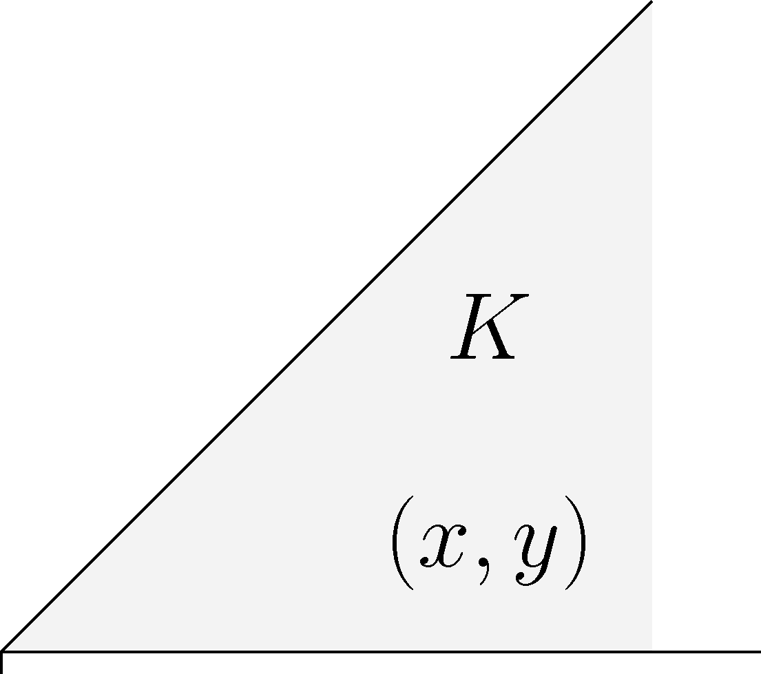
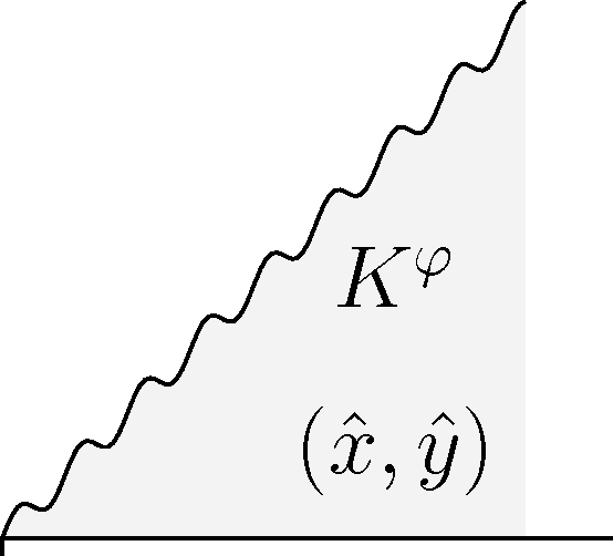
Figure 3. Coordinate transform onto moving domain

Lemma 6.5.

Let $k\in\mathbb{N}$ with $k\geq 1$, $\epsilon\in(0,\frac{\pi}{3(2k+1)})$. Then for any $\varphi\in X_{\epsilon}^{k}$ with $\|\varphi\|_{X_{\epsilon}^{k}}$ sufficiently small, there is a diffeomorphism $\Psi:K\to K^{\varphi}$ of the form

$$\Psi(x,y)\ =\ (x,y)+(0,\psi(x,y))\ =\ (\hat{x},\hat{y}).$$ (6.34)

Furthermore, analogously as in the definition (2.45), there is a decomposition $\psi=\psi_{0}+\psi_{1}$ such that $\psi_{1}=\zeta{\mathcal{P}}$ and where ${\mathcal{P}}$ is a polynomial of order $3k$ such that

$$\sup_{0\leq\ell\leq k}\sum_{|\alpha|=3\ell+2}\|\sup_{0\leq v\leq 1}\big{|}e^{\frac{1}{2}\epsilon|\lambda|(1-v)}\mu^{\ell+1}\Lambda^{\alpha}\widehat{\epsilon\psi_{0}}\big{|}\|_{L^{2}({\Re\lambda=3\ell+\frac{1}{2}})}+\|{\mathcal{P}}\|_{{\mathcal{P}}}\ \leq\ C\|\varphi\|_{X_{\epsilon}^{k}}$$ (6.35)

where we recall that $\mu=\inf\{|\lambda|,\frac{1}{\epsilon}\}$. Furthermore, we have

$$\|\epsilon\psi_{x|\Gamma}\|_{X_{\epsilon}^{k}}+\|\psi_{y|\Gamma}\|_{X_{\epsilon}^{k}}\ \leq\ C\|\varphi\|_{X_{\epsilon}^{k}}.$$ (6.36)

Proof.

We construct $\psi$ to be the solution of

$$\left\{\begin{array}[]{ll}\Delta_{\epsilon}\psi\ =\ 0&\text{in }K,\\ \psi\ =\ \int_{0}^{x}\varphi dx,&\text{on }\partial_{1}K,\\ \psi\ =\ 0,&\text{on }\partial_{0}K.\end{array}\right.$$ (6.40)

As in the previous section, the argument is based on a decomposition the right hand side into a polynomial part and a homogeneous remainder. Since this decomposition proceeds analogously as in the proof of Proposition 6.1 we only consider the case of homogeneous data. That is we assume that $\varphi\in{\stackrel{{\scriptstyle\raisebox{-0.3014pt}[-15.06943pt][-3.01389pt]{\text{\ \tiny oo }}}}{{X}}}_{\epsilon}^{\raisebox{0.0pt}[0.0pt][0.0pt]{\hskip 0.3014pt$\scriptstyle k$}}$. With the transformation (2.43), (6.40) takes the form $\partial_{u}^{2}\psi+({\textstyle\frac{1}{\epsilon}\partial_{v}})^{2}\psi=0$ for $(u,v)\in\mathbb{R}\times(0,1)$. Furthermore, $\psi(u,1)=\int^{u}\varphi e^{\tilde{u}}d\tilde{u}=:H(u)$ and $\psi(u,0)=0$. Application of the Laplace transform in $u$ and since $\lambda\hat{H}(\lambda)=\hat{\varphi}(\lambda-1)$, the solution can be explicitly calculated as (cf. (6.9)-(6.14))

$$\hat{\psi}(\lambda,v)\ =\ \frac{\sin(\epsilon(\lambda)v)}{\sin(\epsilon(\lambda))}\hat{H}(\lambda)\ =\ \frac{1}{\lambda}\frac{\sin(\epsilon(\lambda)v)}{\sin(\epsilon(\lambda))}\hat{\varphi}(\lambda-1).$$ (6.41)

When taking derivatives of (6.41) in $v$, additional factors of $\epsilon\lambda$ are created; furthermore the multiplier has either the cosinus or sinus in the denominator. We have for $v\in(0,1)$,

$$\left|\frac{\sin(\epsilon\lambda v)}{\sin(\epsilon\lambda)}\right|\ \leq\ \left|\frac{\cos(\epsilon\lambda v)}{\sin(\epsilon\lambda)}\right|\ \leq\ \frac{C}{\epsilon\mu}e^{\epsilon|\lambda|(v-1)}\ \leq\ \frac{C}{\epsilon\mu}e^{\frac{1}{2}\epsilon|\lambda|(v-1)}.$$ (6.42)

Indeed, for $|\epsilon\lambda|\leq 1$, we have $\mu=|\lambda|$, $|\frac{\cos(\epsilon\lambda)}{\sin(\epsilon\lambda)}|\leq\frac{C}{|\epsilon\lambda|}=\frac{C}{\epsilon\mu}$ and $|e^{|\epsilon\lambda|(v-1)}|\geq e^{-1}$. For $|\epsilon\lambda|\geq 1$, we have $\mu=\frac{1}{\epsilon}$ (and hence $\frac{1}{\epsilon\mu}=1$) $|\cos(\epsilon\lambda v)|\leq 4e^{|\epsilon\lambda|v}$ and $|\sin(\epsilon\lambda)|\geq\frac{1}{4}e^{|\epsilon\lambda|}$. This proves (6.42). Now, we multiply (6.41) by $|\lambda|^{3k+1}\mu^{k}$, apply the $L^{2}$ norm on the line $\Re\lambda=3\ell-\frac{1}{2}$ and use (6.42). This yields the estimate and in particular uniqueness. This yields (6.35) for (note that $1\leq|\lambda|$ and $1\leq\mu$ for the considered values of $\lambda$). This concludes the proof of (6.35). The estimate of (6.36) follows directly by multiplication of (6.41) with $|\lambda|$ and evaluation at $\Re(\lambda+1)$ (corresponding to one derivative in $x$). ∎

Lemma 6.6.

Let $\Psi$ be the coordinate transform from Lemma 6.5. Then $P:K^{\varphi}\to\mathbb{R}$ is a solution of (6.51) if and only if $p=P\circ\Psi:K\to\mathbb{R}$ satisfies

$$\left\{\begin{array}[]{ll}\Delta_{\epsilon}p\ =\ R(p,\varphi)&\text{ in }K,\\ p\ =\ f_{x}&\text{ on }\partial_{1}K,\\ p_{y}\ =\ 0&\text{ on }\partial_{0}K,\end{array}\right.$$ (6.46)

where the operator $R(p,\varphi)$ is given by (using the notation $\gamma:=(1+\psi_{y})^{-1}$)

$$\begin{aligned} R(p,\varphi)\ =\ &-\gamma_{x}\psi_{x}p_{y}-\gamma\psi_{xx}p_{y}-2\gamma\ \psi_{x}p_{xy}+\gamma\gamma_{y}\psi_{x}^{2}p_{y}\\ &+\gamma^{2}\psi_{x}\psi_{xy}p_{y}+\gamma^{2}\psi_{x}^{2}p_{yy}+({\textstyle\frac{1}{\epsilon}})^{2}\gamma\gamma_{y}p_{y}+({\textstyle\frac{1}{\epsilon}})^{2}(\gamma^{2}-1)p_{yy}.\end{aligned}$$ (6.47)

Proof.

We can write the inverse coordinate transform $\Psi^{-1}:K^{\varphi}\to K$ as $\Psi^{-1}(\hat{x},\hat{y})=(\hat{x},\hat{y}+\eta(\hat{x},\hat{y}))$ for some $\eta:K^{\varphi}\to K$. In particular, $\hat{y}+\eta(\hat{x},\hat{y})+\psi(\hat{x},\hat{y}+\eta(\hat{x},\hat{y}))=\hat{y}$. By differentiating this equality in $\hat{x}$ and $\hat{y}$, we get $\psi_{x}+(1+\psi_{y})\eta_{\hat{x}}=0$ and $(1+\psi_{y})(1+\eta_{\hat{y}})=1$. This implies $\frac{\partial x}{\partial\hat{x}}=1$, $\frac{\partial x}{\partial\hat{y}}=0$, $\frac{\partial y}{\partial x}=-\gamma\psi_{x}$ and $\frac{\partial y}{\partial\hat{y}}=\gamma$, in particular, $P_{\hat{y}}=0\Leftrightarrow P_{y}=0$, justifying the boundary condition in (6.51). Equation (6.47) follows from (6.51) together with

$$P_{\hat{x}\hat{x}}\ =\ (\partial_{x}-\gamma\psi_{t}\partial_{y})(p_{x}-\gamma\psi_{x}p_{y})\$$

$$=\ p_{xx}-\gamma_{x}\psi_{x}p_{y}-\gamma\psi_{xx}p_{y}-2\gamma\ \psi_{x}p_{xy}+\gamma\gamma_{y}\ \psi_{x}^{2}p_{y}+\gamma^{2}\psi_{x}\psi_{xy}p_{y}+\gamma^{2}\psi_{x}^{2}p_{yy},$$

$$P_{\hat{y}\hat{y}}\ =\ \gamma(\gamma\tilde{p}_{y})_{y}\ =\ \gamma^{2}p_{yy}+\gamma\gamma_{y}p_{y}.$$

∎

6.3. Estimates on the pressure

The main result of this section is:

Proposition 6.7 (Shape dependence of $p$).

Let $k\in\mathbb{N}$ with $k\geq 1$, $\epsilon\in(0,\frac{\pi}{3(2k+1)})$ and $\varphi\in X_{\epsilon}^{k-1/2}$, $f\in X_{\epsilon}^{k}$. Then there is a constant $\alpha<1$ such that if $\|\varphi\|_{X_{\epsilon}^{k-1/2}}\leq\alpha$, then there is a unique solution $P:K\to\mathbb{R}$ of

$$\left\{\begin{array}[]{ll}\Delta_{\epsilon}P=0&\text{ in }K^{\varphi},\\ P=f_{x}&\text{ on }\partial_{1}K^{\varphi},\\ P_{y}=0&\text{ on }\partial_{0}K^{\varphi}.\end{array}\right.$$ (6.51)

Furthermore, $p=P\circ\Psi\in Y_{\epsilon}^{k}$ satisfies

$$\|p\|_{Y_{\epsilon}^{k}}\ \leq\ C\|f\|_{X_{\epsilon}^{k}}.$$ (6.52)

Let $q$ be the solution of (6.4) with data $f$ and with right hand side $g=0$. Furthermore, let $\tilde{P}$, $\tilde{p}$ and $\tilde{q}$ be the corresponding solutions with boundary condition $\tilde{f}$ instead of $f$ and let $w=p-q$ and $\tilde{w}=\tilde{p}-\tilde{q}$. Then

$$\|w\|_{Y_{\epsilon}^{k}}\ \leq\ C\|\varphi\|_{X_{\epsilon}^{k-1/2}}\|f\|_{X_{\epsilon}^{k}},$$

$$\|p-\tilde{p}\|_{Y_{\epsilon}^{k}}\ \leq\ C\|\varphi-\tilde{\varphi}\|_{X_{\epsilon}^{k-1/2}}(\|f\|_{X_{\epsilon}^{k}}+\|\tilde{f}\|_{X_{\epsilon}^{k}})+C\|f-\tilde{f}\|_{X_{\epsilon}^{k}},$$ (6.53)

$$\|w-\tilde{w}\|_{Y_{\epsilon}^{k}}\ \leq\ C\|\varphi-\tilde{\varphi}\|_{X_{\epsilon}^{k-1/2}}(\|f\|_{X_{\epsilon}^{k}}+\|\tilde{f}\|_{X_{\epsilon}^{k}})+C\|f-\tilde{f}\|_{X_{\epsilon}^{k}}(\|\varphi\|_{X_{\epsilon}^{k-1/2}}+\|\tilde{\varphi}\|_{X_{\epsilon}^{k-1/2}}).$$

Before we address the proof of Proposition 6.7, we give an estimate of the nonlinear term $R(p,\varphi)$ defined in (6.47):

Proposition 6.8.

Let $k\in\mathbb{N}$, $k\geq 1$, $\epsilon\in(0,\frac{\pi}{3(2k+1)})$. Let $\varphi,\tilde{\varphi}\in X_{\epsilon}^{k-1/2}$ with $\|\varphi\|_{X_{\epsilon}^{k-1/2}}\leq c_{k}$, $\|\tilde{\varphi}\|_{X_{\epsilon}^{k-1/2}}\leq c_{k}$ for some sufficiently small universal constant $c_{k}$. Let $p\in Y_{\epsilon}^{k}$ be the solution of (6.51) on $K^{\varphi}$ with boundary data $f$, let $\tilde{p}\in Y_{\epsilon}^{k}$ be the corresponding solution on $K^{\tilde{\varphi}}$ with boundary data $\tilde{f}$. Then

$$\begin{aligned} \|R(p,\varphi)-R(\tilde{p},\tilde{\varphi})\|_{Z_{\epsilon}^{k}}\ &\leq\ C\|p-\tilde{p}\|_{Y_{\epsilon}^{k}}(\|\varphi\|_{X_{\epsilon}^{k-1/2}}+\|\tilde{\varphi}\|_{X_{\epsilon}^{k-1/2}})\\ &\qquad\qquad+C\|\varphi-\tilde{\varphi}\|_{X_{\epsilon}^{k-1/2}}(\|p\|_{Y_{\epsilon}^{k}}+\|\tilde{p}\|_{Y_{\epsilon}^{k}}),\end{aligned}$$ (6.54)

where $R(p,\varphi)$ is defined in (6.47).

Proof.

The proof uses some ideas of the proof of the algebra property in Lemma 5.4. There are two differences: We also need to take a supremum in the angular variable $v$. The factors in $R$ are controlled by different norms. Furthermore, the norm $g$ controls a discrete set of homogeneous norms (cf. (2.49)). We will show that

$$\|R(p,\varphi)\|_{Z_{\epsilon}^{k}}\ \leq\ C\|\varphi\|_{X_{\epsilon}^{k-1/2}}\|p\|_{Y_{\epsilon}^{k}}$$ (6.55)

the proof of (6.54) follows by an analogous argument, using the multilinear structure of $R$. We use the representation (6.47). Recall the definition (6.40) of the coordinate transform $\psi$. We claim that (6.55) follows by iterative application of

$$\|\rho g\|_{Z_{\epsilon}^{k}}+\|(1-\gamma)g\|_{Z_{\epsilon}^{k}} \leq\ C\|\varphi\|_{X_{\epsilon}^{k-1/2}}\|g\|_{Z_{\epsilon}^{k}},$$ (6.56)

$$\|\rho_{x}w\|_{Z_{\epsilon}^{k}}+\|({\textstyle\frac{1}{\epsilon}}\rho_{y})w\|_{Z_{\epsilon}^{k}}\ \leq\ C\|\varphi\|_{X_{\epsilon}^{k-1/2}}\big{(}\|w_{x}\|_{Z_{\epsilon}^{k}}+\|{\textstyle\frac{1}{\epsilon}}w_{y}\|_{Z_{\epsilon}^{k}}\big{)},$$ (6.57)

where $\rho$ is either one of the terms $\epsilon\psi_{x}$ or $\psi_{y}$ and where we recall that $\gamma=(1+\psi_{y})^{-1}$.

Assuming that (6.56)–(6.57) hold, the proof of (6.55) is easy: Recall that with the definitions of the norms (2.45), (2.49) and by (6.52) we have

$$\|p_{x}\|_{Z_{\epsilon}^{k}}+\|{\textstyle\frac{1}{\epsilon}}p_{y}\|_{Z_{\epsilon}^{k}}+\|p_{xx}\|_{Z_{\epsilon}^{k}}+\|{\textstyle\frac{1}{\epsilon}}p_{xy}\|_{Z_{\epsilon}^{k}}+\|({\textstyle\frac{1}{\epsilon}})^{2}p_{yy}\|_{Z_{\epsilon}^{k}}\ \leq\ C\|p\|_{Y_{\epsilon}^{k}}.$$ (6.58)

We show how the estimate of (6.55) proceeds for the term $\gamma_{x}\psi_{x}p_{y}$ (the first term on the right hand side of (6.47)): In view of $\gamma_{x}=-\gamma^{2}\psi_{xy}$, we have

$$\|\gamma_{x}\psi_{x}p_{y}\|_{Z_{\epsilon}^{k}}\ =\ \|\gamma^{2}(\epsilon\psi_{x})\psi_{xy}({\textstyle\frac{1}{\epsilon}}p_{y})\|_{Z_{\epsilon}^{k}}\ \stackrel{{\scriptstyle\eqref{the-est-1}}}{{\leq}}\ C\|\psi_{xy}({\textstyle\frac{1}{\epsilon}}p_{y})\|_{Z_{\epsilon}^{k}}\stackrel{{\scriptstyle\eqref{the-est-2},\eqref{nochnest}}}{{\leq}}\ C\|\varphi\|_{X_{\epsilon}^{k-1/2}}\|p\|_{Y_{\epsilon}^{.}}$$

Indeed, it can be easily checked that the estimate of the other terms in (6.47) proceeds analogously. In order to conclude the proof of the Proposition, it hence remains to give the argument for (6.56)–(6.57).

Proof of (6.56): In view of the Taylor expansion $\gamma-1=\psi_{y}-\psi_{y}^{2}+\ldots$, the estimate for the term $(1-\gamma)g$ in (6.56) hence follows by the corresponding estimate for the term $\psi_{y}g$ together with the estimate (6.35), $\|\varphi\|_{X_{\epsilon}^{k-1/2}}\leq c_{k}$ and for $c_{k}$ sufficiently small. In order to see (6.56), it hence remains to show

$$\|\rho g\|_{Z_{\epsilon}^{k}}\ \leq\ C\|\varphi\|_{X_{\epsilon}^{k-1/2}}\|g\|_{Z_{\epsilon}^{k}}.$$ (6.59)

Let ${\mathcal{P}}_{\psi}$ and ${\mathcal{P}}_{g}$ be the Taylor polynomials at $(x,y)=(0,0)$ of $\psi$ and $g$ (of order $3k-1$ and $3k-4$, respectively). We decompose $\psi=\psi_{1}+\psi_{0}$ and $g=g_{1}+g_{0}$, where $\psi_{1}:={\mathcal{P}}_{\psi}\zeta$ and $g_{1}:={\mathcal{P}}_{g}\zeta$ and where the radial cut-off function $\zeta=\zeta(|x,y)|)\in C_{c}^{\infty}([0,\infty))$ satisfies $\zeta=1$ in $[0,\frac{1}{8}]$ and $\zeta=0$ in $[\frac{1}{4},\infty]$. The terms $\rho_{0}$ and $\rho_{1}$ are defined correspondingly. Clearly, it is enough to show the corresponding estimate to (6.59) for the products $\rho_{1}g_{1}$, $\rho_{1}g_{0}$, $\rho_{0}g_{1}$ and $\rho_{0}g_{0}$. In the following, we will give the estimate for $\rho_{0}g_{0}$; the estimate of the other terms (related to finite dimensional Taylor expansion) proceeds analogously as in the proof of the algebra property of $X_{\epsilon}^{k}$ in Lemma 5.4. Furthermore, for simplicity of notation, we give the proof with $\Lambda$ replaced by $|\lambda|$ in (2.48), i.e. when only radial derivatives appear . The argument in the case of angular derivatives ${\frac{1}{\epsilon}}\partial_{v}$ proceeds by distributing the derivatives on the two factors using Leibniz’ rule. We will use the notation $K^{|\lambda|}_{\epsilon}=e^{\frac{1}{2}\epsilon|\lambda|(1-v)}$, in particular by the triangle inequality we have $K^{|\lambda|}_{\epsilon}\leq K^{|\lambda-\eta|}_{\epsilon}K^{|\eta|}_{\epsilon}$.

Analogously to (5.6), we decompose the functions $\psi_{0}$ and $g_{0}$ into their low and high frequency part, i.e. $\psi_{0}=\psi_{+}+\psi_{-}$ (with $\rho_{\pm}$ defined correspondingly) and $g_{0}=g_{+}+g_{-}$. In particular, as in (5.7), we have

$$|\lambda|^{k}|\widehat{g_{+}}|+\left({\textstyle\frac{1}{\epsilon}}\right)^{k}|\widehat{g_{-}}|\ \leq\ C\mu^{k}|\widehat{g_{0}}|, |\lambda|^{k}|\widehat{\rho_{+}}|+\left({\textstyle\frac{1}{\epsilon}}\right)^{k}|\widehat{\rho_{-}}|\ \leq\ C\mu^{k}|\widehat{\rho_{0}}|.$$ (6.60)

We need to estimate the terms $g_{+}\rho_{+}$, $g_{+}\rho_{-}$, $g_{-}\rho_{+}$ and $g_{-}\rho_{-}$. We show the estimate for the high frequency/high frequency product $g_{-}\rho_{-}$. Indeed, the estimate for the other two terms proceeds similarly (see also the algebra proof in [26]).

In view of (2.48) and (6.60), we need to show for all $\ell\in[\frac{2}{3},k]$,

$$[\rho_{-}g_{-}]_{{\stackrel{{\scriptstyle\raisebox{-0.3014pt}[-15.06943pt][-3.01389pt]{\text{\ \tiny oo }}}}{{Z}}}_{-}^{\raisebox{0.0pt}[0.0pt][0.0pt]{\hskip 0.21529pt$\scriptstyle\ell$}}}\ =\ C\|\sup_{v\in(0,1)}\big{|}\int_{\Re\eta=\gamma}K^{|\lambda|}_{\epsilon}({\textstyle\frac{1}{\epsilon}})^{\ell}\lambda^{3\ell-2}\widehat{\rho_{-}}(\lambda-\eta)\widehat{g_{-}}(\eta)\ d\Im(\eta)\big{|}\|_{L^{2}({\Re\lambda=3\ell-\frac{7}{2}})}$$

$$\leq\ C\|\varphi\|_{X_{\epsilon}^{k-1/2}}\|g\|_{Z_{\epsilon}^{k}},$$ (6.61)

for any $\gamma\in\mathbb{R}$ of our choice such the above integral is defined. Let $\kappa\in[0,1)$ be the smallest number such that $N:=3\ell-2+\kappa\in\mathbb{N}_{0}$. We show the corresponding stronger estimate to (6.61) where the $\lambda^{3\ell-2}$ is replaced by $\lambda^{N}$. The estimate is stronger since $|\lambda|\geq\frac{1}{2}$ in the line of integration in (6.61). The advantage is that the binomial formula $\lambda^{N}=\sum_{j=0}^{N}\ C_{Nj}(\lambda-\eta)^{j}\eta^{N-j}$ with $N=3\ell-2\in\mathbb{N}_{0}$ can be applied. We have

$$\int_{\Re\lambda=3\ell-\frac{7}{2}}\sup_{v\in(0,1)}\left|\int_{\Re\eta=\gamma}K^{|\lambda|}_{\epsilon}\lambda^{3\ell-2+\kappa}\widehat{\rho_{-}}(\lambda-\eta)\widehat{g_{-}}(\eta)\ d\Im(\eta)\right|^{2}\ d\Im(\lambda)$$

$$=\int_{\Re\lambda=3\ell-\frac{7}{2}}\sup_{v\in(0,1)}\left|\sum_{i=0}^{3\ell-2}C_{Nj}\int_{\Re\eta=\gamma}K^{|\lambda|}_{\epsilon}(\lambda-\eta)^{3\ell-2+\kappa-i}\hat{\rho}_{-}(\lambda-\eta)\eta^{i}\widehat{g_{-}}(\eta)\ d\Im(\eta)\right|^{2}\ d\Im(\lambda).$$

Note that the above inner integrand is analytic in $\eta$ and hence does not depend on the value of $\gamma$ as long as the integral is well-defined; hence we may choose $\gamma$ freely as a function of $i$. In turn, since furthermore $K^{|\lambda|}_{\epsilon}\leq K^{|\lambda-\eta|}_{\epsilon}K^{|\eta|}_{\epsilon}$, it is enough to estimate terms of the form

$$\int_{\Re\lambda=3\ell-\frac{7}{2}}\sup_{v\in(0,1)}\left|\int_{\Re\eta=\gamma}K^{|\lambda-\eta|}_{\epsilon}|\lambda-\eta|^{3\ell+\kappa-2-i}|\widehat{\rho_{-}}(\lambda-\eta)|K^{|\eta|}_{\epsilon}|\eta|^{i}|\widehat{g_{-}}(\eta)|\ d\Im(\eta)\right|^{2}\ d\Im(\lambda)$$ (6.62)

for $\ell\in[\frac{2}{3},k]$, all integers $i\in[0,3\ell-2+\kappa]$ and with our choice of $\gamma\in\mathbb{R}$. We next apply the following variant of (5.10) which says that for all $\tilde{\delta}>\frac{1}{2}$, we have

$$\begin{aligned} \|\sup_{v\in(0,1)}|\hat{F}*\hat{G}|\|_{L^{2}({\Re\lambda=\beta})}\ &\leq\ C_{\delta}\|\sup_{v\in(0,1)}(1+|\lambda|^{\tilde{\delta}})|\hat{F}|\|_{L^{2}({\Re\lambda=\beta_{1}})}\|\sup_{v\in(0,1)}|\hat{G}|\|_{L^{2}({\Re\lambda=\beta_{2}})}\end{aligned}$$ (6.63)

if $\beta_{1}+\beta_{2}=\beta$ and as long as all integrals are well-defined. We introduce the short notation $\|\hat{\varphi}\|_{\Re\lambda=\beta}=\|\sup_{v\in(0,1)}K^{|\lambda|}_{\epsilon}|\hat{\varphi}|\|_{L^{2}({\Re\lambda=\beta})}$. In view of (6.62) and (6.63), for the proof of (6.61) it suffices to show for all $\ell\in[\frac{2}{3},k]$ and for all integers $i\in[0,3\ell-2+\kappa]$,

$$\|(1+|\lambda|^{3\ell+\kappa-2-i+\tilde{\delta}})|\widehat{\rho_{-}}|\|_{\Re\lambda=\beta_{1}}\||\lambda|^{i}\widehat{g_{-}}\|_{\Re\lambda=\beta_{2}}\ \leq\ \|\varphi\|_{X_{\epsilon}^{k-1/2}}\|g\|_{Z_{\epsilon}^{k}},$$ (6.64)

where we can arbitrarily choose $\tilde{\delta}>\frac{1}{2}$ and $\beta_{1},\beta_{2}$ with $\beta_{1}+\beta_{2}=3\ell-\frac{7}{2}$. With the notation $\delta=\tilde{\delta}+(\kappa-1)<\tilde{\delta}$, it is equivalently enough to show .

$$\|(1+|\lambda|^{3\ell-1-i+\delta})|\widehat{\rho_{-}}|\|_{\Re\lambda=\beta_{1}}\||\lambda|^{i}\widehat{g_{-}}\|_{\Re\lambda=\beta_{2}}\ \leq\ \|\varphi\|_{X_{\epsilon}^{k-1/2}}\|g\|_{Z_{\epsilon}^{k}},$$ (6.65)

where we can arbitrarily choose $\delta\geq\frac{1}{2}$ and $\beta_{1},\beta_{2}$ with $\beta_{1}+\beta_{2}=3\ell-\frac{7}{2}$. Both $\beta_{1}$, $\beta_{2}$ as well as $\delta$ are allowed to depend on $\ell$ and $i$. In fact, in the sequel we will always choose $\delta=\frac{1}{2}$.

Recall that either $\rho_{0}=\epsilon\psi_{0x}$ or $\rho_{0}=\psi_{0y}$ and hence either $|\widehat{\rho_{0}}(\lambda)|=|\lambda\widehat{\psi_{0}}(\lambda+1)|$ or $|\widehat{\rho_{0}}(\lambda)|=|\partial_{v}\widehat{\psi_{0}}(\lambda+1)|$. By (6.35) and by the same argument as in the proof of Lemma 5.2, we hence have

$$\|(1+|\lambda|^{3\ell+1}\mu^{\ell+1})|\widehat{\rho_{0}}|\|_{\Re\lambda=3\ell-\frac{1}{2}}\ \leq\ C\|\varphi\|_{X_{\epsilon}^{k-1/2}}, \forall\ell\in[0,k-\tfrac{1}{2}]$$ . (6.66)

By (6.66) and (6.60), we have

$$\|(1+({\textstyle\frac{1}{\epsilon}})^{\ell+1}|\lambda|^{3\ell+1})|\widehat{\rho_{-}}|\|_{\Re\lambda=3\ell-\frac{1}{2}}\ \leq\ C\|\varphi\|_{X_{\epsilon}^{k-1/2}} \forall\ell\in[0,k-\tfrac{1}{2}]$$ . (6.67)

Furthermore, in view of (2.48) and by (6.60), we also have

$$\|({\textstyle\frac{1}{\epsilon}})^{\ell}|\lambda|^{3\ell-2}|\widehat{g_{-}}|\|_{\Re\lambda=3\ell-\frac{7}{2}}\ \leq\ C\|g\|_{Z^{k}_{+}}, \text{$\forall\ell\in[\tfrac{2}{3},k]$}.$$ (6.68)

We prove (6.65) for the three extreme cases, i.e. the corners of the triangle in $(\ell,i)$ where $\ell\in[\frac{2}{3},k]$ and $i\in[0,3\ell-2]\}$, the estimate of the other terms follows by ’interpolation’ of these estimates:

(a1) $\ell=\frac{2}{3}$, $i=0$ (and hence $\beta=3\ell-\frac{7}{2}=-\frac{3}{2}$): With the choice $\beta_{1}=3\cdot\frac{1}{6}-\frac{1}{2}=0$, $\beta_{2}=3\cdot\frac{2}{3}-\frac{7}{2}=-\frac{3}{2}$ and $\delta=\frac{1}{2}$, we need to estimate

$$\|(1+|\lambda|^{\frac{3}{2}})|\widehat{\rho_{-}}|\|_{\Re\lambda=0}\|({\textstyle\frac{1}{\epsilon}})^{\frac{2}{3}}|\widehat{g_{-}}|\|_{\Re\lambda=-\frac{3}{2}}\ \leq\ C\|\varphi\|_{X_{\epsilon}^{k-1/2}}\|g\|_{Z_{\epsilon}^{k}}.$$

(b1) $\ell=k$, $i=0$: With the choice $\beta_{1}=3(k-\frac{1}{2})-\frac{1}{2}=3k-2$, $\beta_{2}=3\cdot\frac{2}{3}-\frac{7}{2}=-\frac{3}{2}$ and $\delta=\frac{1}{2}$, we need to estimate

$$\|(1+|\lambda|^{3k-\frac{1}{2}}({\textstyle\frac{1}{\epsilon}})^{k-\frac{2}{3}})|\widehat{\rho_{-}}|\|_{\Re\lambda=3k-2}\ \|({\textstyle\frac{1}{\epsilon}})^{\frac{2}{3}}|\widehat{g_{-}}|\|_{\Re\lambda=-\frac{3}{2}}\ \leq\ C\|\varphi\|_{X_{\epsilon}^{k-1/2}}\|g\|_{Z_{\epsilon}^{k}}.$$

(c1) $\ell=k$, $i=3k-2$: With the choice $\beta_{1}=3\cdot\frac{1}{6}-\frac{1}{2}=0$, $\beta_{2}=3k-\frac{7}{2}$ and $\delta=\frac{1}{2}$, we need to estimate

$$\|(1+|\lambda|^{\frac{3}{2}})|\widehat{\rho_{-}}|\|_{\Re\lambda=0}\||\lambda|^{3k-2}({\textstyle\frac{1}{\epsilon}})^{k}|\widehat{g_{-}}|\|_{\Re\lambda=3k-\frac{7}{2}}\ \leq\ C\|\varphi\|_{X_{\epsilon}^{k-1/2}}\|g\|_{Z_{\epsilon}^{k}}.$$

Now, using (6.67) and (6.68), it can be easily checked that the above estimates (a1), (b1) and (c1) hold true for $k\geq 1$. This concludes the proof of (6.59) and hence of (6.56).

Proof of (6.57): The proof of (6.57) proceeds similarly to the proof of (6.56). As before, we show the estimate for the crucial high frequency/high frequency case $\rho_{-,x}w_{-}$. With the same arguments as before, we need to show (correspondingly to (6.65)):

$$({\textstyle\frac{1}{\epsilon}})^{k}\||\lambda|^{3\ell-1-i+\kappa}|\widehat{\rho_{-}}|\|_{\Re\lambda=\beta_{1}}\|(1+|\lambda|^{i+\delta})|\widehat{w_{-}}|\|_{\Re\lambda=\beta_{2}}\$$

$$\leq\ C\|\varphi\|_{X_{\epsilon}^{k-1/2}}\big{(}\|w_{x}\|_{Z_{\epsilon}^{k}}+\|{\textstyle\frac{1}{\epsilon}}w_{y}\|_{Z_{\epsilon}^{k}}\big{)}\ =:\ \mathcal{R},$$ (6.69)

(we have put the $\delta$ on the second factor). In the above inequality, we can arbitrarily choose $\beta_{1},\beta_{2}$, $\delta$ as long as $\beta_{1}+\beta_{2}=3\ell-\frac{5}{2}$ and $\delta\geq\frac{1}{2}$. Both $\beta_{1}$, $\beta_{2}$ as well as $\delta$ may depend on $\ell$, $i$. We note that by (2.48), we have

$$\|({\textstyle\frac{1}{\epsilon}})^{\ell}|\lambda|^{3\ell-1}|\widehat{w_{-}}|\|_{\Re\lambda=3\ell-\frac{5}{2}}\ \leq\ C\big{(}\|w_{x}\|_{Z^{k}_{+}}+\|{\textstyle\frac{1}{\epsilon}}w_{y}\|_{Z^{k}_{+}}\big{)}, \text{$\forall\ell\in[\tfrac{1}{2},k]$}.$$ (6.70)

We prove (6.3) in the case when the maximum number of derivatives fall onto $\rho$, i.e. $\ell=k$ and $i=0$ (in particular, $\kappa=0$ where we recall that $\kappa$ is defined as the smallest nonnegative integer such that $3\ell-2\in\mathbb{N}$). With the choice $\beta_{1}=3(k-\frac{1}{2})-\frac{1}{2}=3k-2$, $\beta_{2}=3\cdot 1-\frac{5}{2}=\frac{1}{2}$ and $\delta=1$, we hence need to estimate

$$\|({\textstyle\frac{1}{\epsilon}})^{k}|\lambda|^{3k-1}|\widehat{\rho_{-}}|\|_{\Re\lambda=3k-2}\ \|(1+|\lambda|)({\textstyle\frac{1}{\epsilon}})^{\frac{2}{3}}|\widehat{g_{-}}|\|_{\Re\lambda=\frac{1}{2}}\ \leq\ C\mathcal{R}.$$

This estimate holds true as can easily be checked using (6.67) and (6.70). The estimate of the terms $\rho_{-,x}w_{-}$, $\rho_{-,x}w_{-}$ and $\rho_{-,x}w_{-}$ proceeds similarly. This concludes the estimate of (6.57) and hence of the proposition. ∎

Proof of Proposition 6.7.

We first show the existence of a solution $P$ of (6.51) on $K^{\varphi}$. By Lemma 6.6, for this we need to find a solution $p$ of (6.46). We will solve (6.46) using an iterative argument. We set $p_{0}:=0$ and iteratively define $p_{i+1}$ to be the solution of (6.4) with right hand side $g=R(p_{i-1},\varphi)$ and boundary data $f_{x}$. By (6.5) and (6.54), we get

$$\|p_{i+1}-p_{i}\|_{Y_{\epsilon}^{k}}\ \stackrel{{\scriptstyle\eqref{est-p}}}{{\leq}}\ C\|R(p_{i},\varphi)-R(p_{i-1},\varphi)\|_{Z_{\epsilon}^{k}}\ \stackrel{{\scriptstyle\eqref{einfach}}}{{\leq}}\ C\|\varphi\|_{Y_{\epsilon}^{k-1/2}}\|p_{i+1}-p_{i}\|_{Y_{\epsilon}^{k}}$$

$$\leq\ \ C\alpha\|p_{i+1}-p_{i}\|_{Y_{\epsilon}^{k}}\ \leq\ \ \tfrac{1}{2}\|p_{i+1}-p_{i}\|_{Y_{\epsilon}^{k}}$$

for $\alpha$ sufficiently small, $\{p_{i}\}_{i\in\mathbb{N}}$ is a Cauchy sequence and converges to a solution $p$ of (6.46). By (6.5), $p$ satisfies (6.52). The estimates (6.7) now follow from the representation (6.46) of the solution together with the estimates (6.54) and (6.55). ∎

We also have the nonlinear version of the trace estimate in Lemma 6.4:

Lemma 6.9.

Suppose that the assumptions of Proposition 6.7 are satisfied (in particular, $k\geq 1$). Then with the notation of Proposition 6.7, we have

$$\|\partial_{x}(p_{x})_{|\Gamma}\|_{X_{\epsilon}^{k-1}}+({\textstyle\frac{1}{\epsilon}})^{2}\|\partial_{x}(p_{y})_{|\Gamma}\|_{X_{\epsilon}^{k-1}}\ \leq\ C\|f\|_{X_{\epsilon}^{k}}.$$ (6.71)

Proof.

Indeed, (6.71) follows by application of (6.26) and since $p$ satisfies (6.46). ∎

Note that the corresponding ’bilinear’ estimates for $w$, $p-\tilde{p}$ and $w-\tilde{w}$ also hold (correspondingly as in Proposition 6.7): The estimates for the case of $x$ derivative are

$$\|\partial_{x}(w_{x})_{|\Gamma}\|_{X_{\epsilon}^{k-1}}\ \leq\ C\|\varphi\|_{X_{\epsilon}^{k-1/2}}\|f\|_{X_{\epsilon}^{k}},$$

$$\|\partial_{x}(p_{x})_{|\Gamma}-\partial_{x}(\tilde{p}_{x})_{|\Gamma}\|_{X_{\epsilon}^{k-1}}\ \leq\ C\|\varphi-\tilde{\varphi}\|_{X_{\epsilon}^{k-1/2}}(\|f\|_{X_{\epsilon}^{k}}+\|\tilde{f}\|_{X_{\epsilon}^{k}})+C\|f-\tilde{f}\|_{X_{\epsilon}^{k}},$$ (6.72)

$$\|\partial_{x}(w_{x})_{|\Gamma}-\partial_{x}(\tilde{w}_{x})_{|\Gamma}\|_{X_{\epsilon}^{k-1}}\ \leq\ C\|\varphi-\tilde{\varphi}\|_{X_{\epsilon}^{k-1/2}}(\|f\|_{X_{\epsilon}^{k}}+\|\tilde{f}\|_{X_{\epsilon}^{k}})$$

$$\qquad+C\|f-\tilde{f}\|_{X_{\epsilon}^{k}}(\|\varphi\|_{X_{\epsilon}^{k-1/2}}+\|\tilde{\varphi}\|_{X_{\epsilon}^{k-1/2}}).$$

These estimates follow analogously to (6.71) but by using the ’bilinear’ estimates (6.54) for $R$. The corresponding estimates to (6.3) with $\partial_{x}(w_{x})_{|\Gamma}$ and $\partial_{x}(\tilde{p}_{x})_{|\Gamma}$ replaced by $({\textstyle\frac{1}{\epsilon}})^{2}\partial_{x}(w_{y})_{|\Gamma}$ and $({\textstyle\frac{1}{\epsilon}})^{2}\partial_{x}(w_{y})_{|\Gamma}$, respectively, also hold.

6.4. Estimates for the profile

In this section, we prove Proposition 4.2. We show that

$$\|N_{\epsilon}(f)\|_{TX_{\epsilon}^{k}}+\|N_{\epsilon}(f)\|_{L^{2}(X_{\epsilon}^{0})}\ \leq\ C\|f\|_{TX_{\epsilon}^{k+1}}^{2}.$$ (6.73)

The proof of (4.2) then follows by a straightforward extension of this estimate (indeed the estimates (6.54) show that the main part $\partial_{x}{\mathcal{B}}_{\epsilon}\partial_{x}$ of the operator ${\mathcal{N}}_{\epsilon}$ can be estimated like a bilinear operator). We recall,

$$N_{\epsilon}(f) =\ \frac{f_{x}}{(1+\epsilon^{2})^{\frac{3}{2}}}\bigg{(}\frac{f_{xx}-3\epsilon^{2}f_{x}^{2}}{1+\epsilon^{2}}\bigg{)}_{|x=0}+\partial_{x}B_{\epsilon}^{f}\bigg{(}\frac{f_{x}}{(1+\epsilon^{2}(1+f)^{2})^{\frac{3}{2}}}\bigg{)}+A_{\epsilon}f,$$

cf. (2.27). The two main estimates in favor of (6.73) are:

$$\|f_{xx|x=0}f_{x}\|_{TX_{\epsilon}^{k}}+\|f_{xx|x=0}f_{x}\|_{L^{2}(X_{\epsilon}^{k})}\ \leq\ C\|f\|_{TX_{\epsilon}^{k+1}}^{2},$$ (6.74)

$$\|\partial_{x}B_{\epsilon}^{f}\partial_{x}f+A_{\epsilon}f\|_{TX_{\epsilon}^{k}}+\|\partial_{x}B_{\epsilon}^{f}\partial_{x}f+A_{\epsilon}f\|_{TX_{\epsilon}^{k}}\ \leq\ C\|f\|_{TX_{\epsilon}^{k+1}}^{2}.$$ (6.75)

Two “nonlinear” corrections have been neglected in the estimates (6.74) and (6.75): One correction is related to the $-3\epsilon^{2}f_{x}^{2}|_{|x=0}$ term, the other correction is related to the term $f_{x}((1+\epsilon^{2}(1+f)^{2})-1)$. Indeed, these corrections are easily controlled as lower order terms for sufficiently small $f$; the estimate of these terms is left to the reader. In the following, we will give the proof of (6.74) and (6.75).

Proof of (6.74): In view of the definition (2.39), (6.74) follows from

$$[\partial_{t}^{i}(f_{xx|x=0}f_{x})]_{L^{2}(X_{\epsilon}^{j})}\ \leq\ C\|f\|_{TX_{\epsilon}^{k+1}}^{2}, 0\leq i+j\leq k$$ for . (6.76)

In order to see (6.76), we note that by (5.2), we have

$$\|f_{xx|x=0}f_{x}\|_{X_{\epsilon}^{0}}\ =\ \|f_{xx|x=0}f_{x}\|_{L^{2}}\ \leq\ \|f_{x}\|_{L^{2}}\|f_{xx}\|_{L^{\infty}}\ \stackrel{{\scriptstyle\eqref{X-sob}}}{{\leq}}\ C\|f\|_{X_{\epsilon}^{1/2}}\|f\|_{X_{\epsilon}^{1}},$$ (6.77)

$$\|f_{xx|x=0}f_{x}\|_{X_{\epsilon}^{j}}\ \leq\ \|f_{x}\|_{X_{\epsilon}^{j}}\|f_{xx}\|_{L^{\infty}}\ \stackrel{{\scriptstyle\eqref{X-three}}}{{\leq}}\ C\|f\|_{X_{\epsilon}^{j}}\|f\|_{X_{\epsilon}^{j+1}}\qquad\text{for $1\leq j\leq k$}.$$ (6.78)

We take the square of (6.77) and integrate the equation in time. We then apply Hölders inequality with $L^{2}$ on the $\|\cdot\|_{X_{\epsilon}^{1}}$ term and $L^{\infty}$ on the $\|\cdot\|_{X_{\epsilon}^{1/2}}$ term. In view of (5.12), this yields (6.76) for $i=j=0$. The estimate for $i>0$ or $j>0$ follows from (6.78): We take the square of (6.78) and integrate in time. We then apply Hölder’s inequality with $L^{2}$ on the $\|\cdot\|_{X_{\epsilon}^{j+1}}$ term and $L^{\infty}$ on the $\|\cdot\|_{X_{\epsilon}^{j}}$ term. In view of (5.12), this yields (6.76) for $i=0$ and $1\leq j\leq k$. It remains to prove (6.76) for $i>0$: In this case we note that the time derivatives on the left hand side of (6.76) are distributed according to Leibniz’ rule on the two factors. The loss of regularity due to the time derivation is compensated by the fact that we only need to estimate the smaller norm $j=\ell-i$. In view of the definition of $\|\cdot\|_{TX_{\epsilon}^{k+1}}$, this yields (6.76) for all $0\leq i\leq\ell$ and $j\geq 1$. This concludes the proof of (6.74).

Proof of (6.75): With the same argument as before, the proof of (6.75) can be reduced to the following estimate which does not involve time:

$$[\partial_{x}B_{\epsilon}^{f}\partial_{x}f+A_{\epsilon}f]_{X_{\epsilon}^{j}}\ \leq\ C\|f\|_{X_{\epsilon}^{j+1/2}}\|f\|_{X_{\epsilon}^{j+1}} \text{for $0\leq j\leq k$},$$ (6.79)

where we may assume that $\|f\|_{X_{\epsilon}^{k+1/2}}\leq\alpha\leq 1$ (this corresponds to the estimate $\|f\|_{C^{0}(X_{\epsilon}^{k-1/2})}\leq\alpha\leq 1$ for the corresponding time-space estimate). Let $\psi$, $\gamma$ be defined in Lemma 6.5 and let $p$, $q$ be defined as in Proposition 6.7. By (2.26), (2.24) and (2.14), we have

$$A_{\epsilon}f_{x}\ =\ (1+\epsilon^{2})^{-\frac{3}{2}}\partial_{x}\big{[}q_{x}-({\textstyle\frac{1}{\epsilon}})^{2}q_{y}\big{]}_{|\Gamma},$$

$$-\partial_{x}B_{\epsilon}^{f}f_{x}\ =\ (1+\epsilon^{2})^{-\frac{3}{2}}\partial_{x}\big{[}(1+f)\ (p_{x}-\gamma\psi_{x}p_{y})-({\textstyle\frac{1}{\epsilon}})^{2}\gamma p_{y}\big{]}_{|\Gamma}.$$

With the notation $w=p-q$ and $C_{\epsilon}=(1+\epsilon^{2})^{-3/2}\leq 1$, we hence get

$$A_{\epsilon}f+\partial_{x}B_{\epsilon}^{f}f_{x}\ =\ C_{\epsilon}\partial_{x}\Big{[}({\textstyle\frac{1}{\epsilon}})^{2}w_{y}-w_{x}-fp_{x}+(1+f)\gamma\psi_{x}p_{y}+({\textstyle\frac{1}{\epsilon}})^{2}(\gamma-1)p_{y}\Big{]}_{|\Gamma}.$$ (6.80)

We first note that for all $j\geq 0$, we have

$$\|(w_{x|\Gamma})_{x}\|_{X_{\epsilon}^{j}}+\|({\textstyle\frac{1}{\epsilon}})^{2}(w_{y|\Gamma})_{x}\|_{X_{\epsilon}^{j}}\ \stackrel{{\scriptstyle\eqref{nl-trace-2}}}{{\leq}}\ \ C\|f\|_{X_{\epsilon}^{j+1/2}}\|f\|_{X_{\epsilon}^{j+1}}.$$ (6.81)

For the other terms on the right hand side of (6.80) and for $j\geq 1$ we additionally use the algebra property (5.8). The estimate of the term $f(p_{x|\Gamma})_{x}$ proceeds as follows

$$\|(fp_{x|\Gamma})_{x}\|_{X_{\epsilon}^{j}}\ \stackrel{{\scriptstyle\eqref{X-alg}}}{{\leq}}\ \|f_{x}\|_{X_{\epsilon}^{j}}\|p_{x|\Gamma}\|_{X_{\epsilon}^{j}}+\|f\|_{X_{\epsilon}^{j}}\|(p_{x|\Gamma})_{x}\|_{X_{\epsilon}^{j}}\ \stackrel{{\scriptstyle\eqref{X-three},\eqref{nl-trace-1}}}{{\leq}}\ C\|f\|_{X_{\epsilon}^{j+1/2}}\|f\|_{X_{\epsilon}^{j+1}},$$

where we also used $\|p_{x|\Gamma}\|_{L^{2}}\leq C\|p\|_{Y_{\epsilon}^{1}}\ \leq C\|f\|_{X_{\epsilon}^{1}}$ which follows from (5.11) and (6.52). We also note that in view of (6.36) we have $\|\epsilon\psi_{x|\Gamma}\|_{X_{\epsilon}^{k+1/2}}+\|\psi_{y|\Gamma}\|_{X_{\epsilon}^{k+1/2}}\leq C\alpha<1$ if the constant $\alpha$ in the assumption of Theorem 3.1 is chosen sufficiently small. In view of the Taylor expansion $1-\gamma=\psi_{y}-\psi_{y}^{2}+\ldots$ and by (6.36), this implies also $\|\gamma_{|\Gamma}-1\|_{X_{\epsilon}^{j}}\leq\|\psi_{y|\Gamma}\|_{X_{\epsilon}^{j}}\leq C$. For $j\geq 1$, the estimate of the remaining terms in (6.80) then follows using these estimates together with (5.8), (6.36) and (6.71).

It remains to give the estimate for $j=0$, where the algebra property (5.8) does not apply: We show the estimate for the nonlinear term $(fp_{x|\Gamma})_{x}$, the estimate for the other terms proceeds analogously. Indeed, we have

$$\|(fp_{x|\Gamma})_{x}\|_{L^{2}}\ \leq\ \|f\|_{L^{\infty}}\|(p_{x|\Gamma})_{x}\|_{L^{2}}+\|f_{x}\|_{L^{2}}\|p_{x|\Gamma}\|_{L^{\infty}}\ \stackrel{{\scriptstyle\eqref{nl-trace-1}}}{{\leq}}\ C\|f\|_{X_{\epsilon}^{1/2}}\|f\|_{X_{\epsilon}^{1}},$$

where we also used $\|p_{x|\Gamma}\|_{L^{2}}\leq C\|p\|_{Y_{\epsilon}^{1}}\ \leq C\|f\|_{X_{\epsilon}^{1}}$ which follows from (5.11) and (6.52). The estimate of the other terms proceeds analogously. This concludes the proof of (6.79) and hence of the lemma.

7. Localization argument

We prove Propositions 4.4-4.5 thus concluding the proof of Theorem 3.3 in Section 4. We will use the notation used in the proof of this theorem. We first note that the derivative ${\delta\mathcal{L}}_{\epsilon}^{w}$ of $\mathcal{L}_{\epsilon}$ at $w$ is given by

$${\delta\mathcal{L}}_{\epsilon}^{w}f\ =\ L_{\epsilon}^{w}f+K_{\epsilon}^{w}f,$$ (7.1)

cf. (2.15), where the operators $L_{\epsilon}$ (leading order) and $K_{\epsilon}^{w}$ (remainder) are given by

$$\displaystyle L_{\epsilon}^{w}f\ =\ f_{t}-\frac{1}{(1+\epsilon^{2})^{3/2}}\big{(}B_{\epsilon}^{w}f_{x}\big{)}_{x}\ =:\ f_{t}+A^{w}_{\epsilon}f$$ (7.2)

and

$$K_{\epsilon}^{w}f\ =\ (D^{w}-1)f_{t}+\dot{D}^{w}f+\partial_{t}({\mathcal{D}}^{w}fw)$$ (7.3)

$$\qquad-\big{[}\big{(}(1-x)\dot{s}_{-}+x\dot{s}_{+}\big{)}f\big{]}_{x}-\big{[}\big{(}(1-x)\dot{\sigma}_{-}^{w}+x\dot{\sigma}_{+}^{w}\big{)}w\big{]}_{x}$$ (7.4)

$$\qquad-\Big{[}B_{\epsilon}^{w}\big{(}\frac{3w_{x}(2\epsilon^{2}w_{x}f)}{2(1+\epsilon^{2}(w+f^{*})^{2})^{\frac{5}{2}}}\big{)}\Big{]}_{x}+\Big{[}\delta B_{\epsilon}^{w}\big{(}f,\frac{w_{x}}{(1+\epsilon^{2}w^{2})^{\frac{3}{2}}}\big{)}\Big{]}_{x}.$$

Here, we have introduced the following notation: $s_{\pm}^{w}(t)$ is defined as in (2.16) with $f$ replaced by $w$; $D^{w}$ is defined as in (2.7) with $s_{\pm}(t)$ replaced by $s_{\pm}^{w}(t)$. Furthermore $\mathcal{D}^{w}f=\delta D^{w}(f)$ and $\sigma_{\pm,w}f=\delta s_{\pm,w}(f)$ are the linearizations of $D^{w}$, $\sigma_{\pm,w}$. Furthermore, $\delta B^{w}$ denotes the shape derivative of $B^{w}$ (derivative in $w$ direction). A dot on the top of a symbol denotes the time derivative.

The proof is based on two small parameters $\delta,\tau>0$. The parameter $\delta$ is used to localize the estimates near the boundary. Note that in the interior where $C>h>c>0$, the operator is uniformly parabolic. The parameter $\tau$ signifies the time integral where the solution is defined. In the course of the proof, we will choose $\delta$ and $\tau=\tau(\delta)$, in this order, to be sufficiently small. In this section, we write $c$, $C$ for all constants which depend only on $f_{\rm in},k$, but neither depend on $\delta$ nor $\tau$.

For $\delta>0$, we define a covering of $E=(0,1)$ by setting $E_{1\delta}:=(0,2\delta),E_{2\delta}:=(\delta,1-\delta),E_{3\delta}:=(1-2\delta,1)$. Correspondingly, let $Q_{i\delta\tau}:=(0,\tau)\times E_{i\delta}$. We choose a smooth partition of unity $\{\psi_{i\delta}\}_{i=1,2,3}$, subordinate to this covering with $\psi_{i\delta}\in C_{c}^{\infty}(\overline{E}_{i\delta},[0,1])$, $\sum_{i}\psi_{i\delta}=1$ on $E$ and also $\|\partial^{j}\psi_{i\delta}\|_{L^{\infty}}\leq C\delta^{-j}$ for all $j\geq 0$. We also define a second set of cut-off functions $\{\tilde{\psi}_{i\delta}\}_{i=1,2,3}$: Let $\tilde{E}_{1\delta}:=(0,4\delta),\tilde{E}_{2\delta}:=(3\delta,1-3\delta),\tilde{E}_{3\delta}:=(1-4\delta,1)$. We choose $\psi_{1\delta}\in C_{c}^{\infty}(\overline{E}_{i\delta},[0,1])$ with $\tilde{\psi}_{i\delta}=1$ in $E_{i\delta}$ and in particular, $\tilde{\psi}_{i\delta}\psi_{i\delta}=\psi_{i\delta}$. Finally, we also consider the cut-off function $\hat{\psi}_{1\delta}$, supported on an even larger set such that $\hat{\psi}_{1\delta}\tilde{\psi}_{1\delta}=\tilde{\psi}_{1\delta}$. The support of $\hat{\psi}_{1\delta}=1$ is e.g. included in $(0,5\delta)$, the functions $\hat{\psi}_{2\delta},\hat{\psi}_{3\delta}$ are defined analogously.

Since $\|f_{\rm in}\|_{X_{\epsilon}^{3/2}({E})}<C$ and $\|w\|_{TX_{\epsilon}^{2}({Q_{\tau}})}<C$, it follows that $f_{\rm in}$ and $w$ are Hölder continuous in time and space. Therefore, by the boundary condition $|h_{\rm in,x}(0)|=|h_{\rm in,x}(1)|=1$ and recalling that $h_{\rm in}=x(1-x)+\int_{0}^{x}f_{\rm in}(x^{\prime})dx^{\prime}$, there is $\delta_{0}>0$ such that for all $\delta<\delta_{0}$ we have $|\partial_{x}h_{0}|\in(\frac{1}{2},2)$ in $E_{1\delta}\cap E_{3\delta}$ and $h_{0}\in(c,C)$ in $E_{2\delta}$. Similarly, there is $\delta_{0}$ and $\tau_{0}$ such that the corresponding estimates hold for $h^{w}(\tau)=x(1-x)+\int_{0}^{x}w(\tau,x^{\prime})dx^{\prime}$ for all $\delta<\delta_{0}$ and every fixed time $\tau<\tau_{0}$. In the sequel, we will always assume $0<\delta,\tau<\min\{\delta_{0},\tau_{0},0.1\}$.

7.1. Proof of Proposition 4.4

Proof of Proposition 4.4.

In view of the extension Lemma 4.3, we only need to consider the case of zero initial data so that in the following we may assume $f_{\rm in}=0$. We begin with the proof of maximal regularity estimate (4.13). That is we assume that $f$ satisfies

$$\delta{\mathcal{L}}_{\epsilon}^{w}f\ =\ g\ \ \text{in }Q_{\tau} f\ =\ 0\quad\text{on $(0,\tau)\times\partial E$}$$ and (7.5)

and with initial data $f=0$ and we will show

$$\|f\|_{TX_{\epsilon}^{k+1}({Q_{\tau}})}\ \leq\ C\|g\|_{TX_{\epsilon}^{k}({Q_{\tau}})}.$$ (7.6)

With the partition of unity $\psi_{i\delta}$, $i=1,2,3$ and by the triangle inequality, we have

$$\|f\|_{TX_{\epsilon}^{k+1}({Q_{\tau}})}\ \leq\ \|\psi_{1\delta}f\|_{TX_{\epsilon}^{k+1}({Q_{\tau}})}+\|\psi_{2\delta}f\|_{TX_{\epsilon}^{k+1}({Q_{\tau}})}+\|\psi_{3\delta}f\|_{TX_{\epsilon}^{k+1}({Q_{\tau}})}.$$ (7.7)

We begin with the estimate for $\psi_{1\delta}f$ (related to the left boundary of the domain). The idea is to use that on $Q_{1\delta\tau}$ (that is near the left boundary), $\partial{\mathcal{L}}$ (and also $L_{\epsilon}^{w}$) are approximated by $L_{\epsilon}$, where $L_{\epsilon}f:=f_{t}+A_{\epsilon}f$ and where $A_{\epsilon}$ is defined in (2.26). We first claim that

$$\|\psi_{1\delta}f\|_{TX_{\epsilon}^{k+1}({Q_{\tau}})} \leq C_{\delta}\|\tilde{\psi}_{1\delta}L_{\epsilon}(\psi_{1\delta}f)\|_{TX_{\epsilon}^{k}({Q_{\tau}})}+C_{\delta}\|f\|_{TX_{\epsilon}^{k}({Q_{\tau}})}+\frac{1}{10}\|f\|_{TX_{\epsilon}^{k+1}({Q_{\tau}})},$$ (7.8)

where we recall $\tilde{\psi}_{1\delta}\psi_{1\delta}=\psi_{1\delta}$ and hence $(1-\tilde{\psi}_{1\delta})\psi_{1\delta}=0$. In order to see (7.8), we first note that by (4.2), we get $\|\psi_{1\delta}f\|_{TX_{\epsilon}^{k+1}({Q_{\tau}})}\leq C\|L_{\epsilon}\psi_{1\delta}f\|_{TX_{\epsilon}^{k}({(0,\tau)\times K})}$ (the $L^{2}$-term is estimated by the other term since the support of the right hand side is bounded). Furthermore,

$$L_{\epsilon}(\psi_{1\delta}f)\ =\ \tilde{\psi}_{1\delta}L_{\epsilon}(\psi_{1\delta}f)+(1-\tilde{\psi}_{1\delta})L_{\epsilon}(\psi_{1\delta}f)$$

$$=\ \tilde{\psi}_{1\delta}A_{\epsilon}(\psi_{1\delta}f)+\psi_{1\delta}f_{t}+(1-\tilde{\psi}_{1\delta})A_{\epsilon}(\psi f).$$

Furthermore, by (2.26) and since $\tilde{\psi}_{1\delta}$ depends only on $x$, by a short calculation we obtain

$$A_{\epsilon}(\psi_{1\delta}f) =\partial_{x}(-p^{\prime}_{x}+\frac{1}{\epsilon^{2}}p^{\prime}_{y}),$$

$$(1-\tilde{\psi}_{1\delta})A_{\epsilon}(\psi_{1\delta}f) =\partial_{x}(-\tilde{p}^{\prime}_{x}+\frac{1}{\epsilon^{2}}\tilde{p}^{\prime}_{y})-\partial_{xx}\tilde{\psi}_{1\delta}p^{\prime}-2\partial_{x}\tilde{\psi}_{1\delta}p^{\prime}_{x}+\frac{1}{\epsilon^{2}}\partial_{x}\tilde{\psi}_{1\delta}p^{\prime}_{y},$$

where $p^{\prime}:K\to\mathbb{R}$ and $\tilde{p}^{\prime}:=(1-\tilde{\psi}_{1\delta})p^{\prime}$ are the solutions of

$$\left\{\begin{array}[]{ll}\Delta_{\epsilon}p^{\prime}=0&\text{ in }K,\\ p^{\prime}=(\psi_{1\delta}f)_{x}&\text{ on }\Gamma=\partial_{1}K,\\ p^{\prime}_{y}=0&\text{ on }\partial_{0}K.\end{array}\right. \left\{\begin{array}[]{ll}\Delta_{\epsilon}\tilde{p}^{\prime}=-2\partial_{x}\tilde{\psi}_{1\delta}p^{\prime}_{x}-\partial_{x}^{2}\tilde{\psi}_{1\delta}p^{\prime}&\text{ in }K,\\ \tilde{p}^{\prime}=0&\text{ on }\partial_{1}K,\\ \tilde{p}^{\prime}_{y}=0&\text{ on }\partial_{0}K.\end{array}\right.$$ (7.15)

In the following, we use the following Rellich-type estimate for lower order terms which can be obtained by standard interpolation: For any given $\delta>0$, we have

$$\|f_{xx}\|_{X_{\epsilon}^{k-1}}\ \leq\ \delta\|f\|_{X_{\epsilon}^{k}}+C_{\delta}\|f\|_{X_{\epsilon}^{k-1}}.$$ (7.16)

Using this inequality, estimate (7.8) follows by application of Proposition 6.1.

Let $[L_{\epsilon}^{w},\psi_{1\delta}]:=L_{\epsilon}^{w}\psi_{1\delta}-\psi_{1\delta}L_{\epsilon}^{w}$ denote the commutator of $L_{\epsilon}^{w}$ and $\psi_{1\delta}$, then

$$\|\tilde{\psi}_{1\delta}L_{\epsilon}(\psi_{1\delta}f)\|_{TX_{\epsilon}^{k}({Q_{\tau}})}\leq\|\tilde{\psi}_{1\delta}(L_{\epsilon}-\delta{\mathcal{L}}_{\epsilon}^{w})(f\psi_{1\delta})\|_{TX_{\epsilon}^{k}({Q_{\tau}})}+\|\tilde{\psi}_{1\delta}\delta{\mathcal{L}}_{\epsilon}^{w}(\psi_{1\delta}f)\|_{TX_{\epsilon}^{k}({Q_{\tau}})}$$

$$\leq\|\tilde{\psi}_{1\delta}(L_{\epsilon}-\delta{\mathcal{L}}_{\epsilon}^{w})(f\psi_{1\delta})\|_{TX_{\epsilon}^{k}({Q_{\tau}})}+\|\tilde{\psi}_{1\delta}[\delta{\mathcal{L}}_{\epsilon}^{w},\psi_{1\delta}]f\|_{TX_{\epsilon}^{k}({Q_{\tau}})}+\|\psi_{1\delta}g\|_{TX_{\epsilon}^{k}({Q_{\tau}})},$$ (7.17)

where we have used $\psi_{1\delta}\tilde{\psi}_{1\delta}=\psi_{1\delta}$. The estimate of the first and second term on the right-hand side of the above estimate is given in Lemmas 7.1 and 7.2. Choosing $\delta$ sufficiently small, we hence obtain

$$\|\psi_{1\delta}f\|_{TX_{\epsilon}^{k+1}({Q_{\tau}})} \leq\ C_{\delta}\|g\|_{TX_{\epsilon}^{k}({Q_{\tau}})}+C_{\delta}\|f\|_{TX_{\epsilon}^{k}({Q_{\tau}})}+\frac{1}{6}\ \|f\|_{TX_{\epsilon}^{k+1}({Q_{\tau}})}.$$

The third term on the right hand side of (7.7) can be estimated analogously. For the middle term (corresponding to the interior of the domain), we note that in the interior, our weighted Sobolev norms are equivalent to standard Sobolev norms (with equivalence depending on $\delta$) and an analogous estimate to the one above can be achieved for the middle term using standard parabolic estimates, see also [16, 29]. Altogether, these estimates yield

$$\|f\|_{TX_{\epsilon}^{k+1}({Q_{\tau}})}\ \stackrel{{\scriptstyle\eqref{split}}}{{\leq}}\ C_{\delta}\|g\|_{TX_{\epsilon}^{k}({Q_{\tau}})}+C_{\delta}\|f\|_{TX_{\epsilon}^{k}({Q_{\tau}})}+\frac{1}{2}\|f\|_{TX_{\epsilon}^{k+1}({Q_{\tau}})}.$$

Then using that $f_{|t=0}=0$, we deduce that $\|f\|_{TX_{\epsilon}^{k}({Q_{\tau}})}\leq C\tau^{1/2}\|f\|_{TX_{\epsilon}^{k+1}({Q_{\tau}})}$ and we choose $\tau$ such that $C_{\delta}C\tau^{1/2}<\frac{1}{6}$. Hence,

$$\|f\|_{TX_{\epsilon}^{k+1}({Q_{\tau}})}\ \stackrel{{\scriptstyle\eqref{split}}}{{\leq}}\ C_{\delta}\|{\delta\mathcal{L}}_{\epsilon}^{w}f\|_{TX_{\epsilon}^{k}({Q_{\tau}})}+\frac{1}{2}\|f\|_{TX_{\epsilon}^{k+1}({Q_{\tau}})},$$

which yields (7.6) by absorbing on the left hand side.

The existence part is similar to the proof of Lemma 3.4 of [20]. Indeed, the argument used there can be generalized since only very little of the particular structure is used: The main ingredient in this argument is existence and maximal regularity for the linearized operator at the boundary. The second ingredient is the fact that existence of a solution together with estimates in the interior follows by standard parabolic theory. We have already proved these properties for our operator. Finally, the argument also requires that the operator can be localized in the sense that the long-range interaction of the solution operator only yields a lower order contribution. Indeed, we have used this idea already in the proof of (7.8). ∎

In the following we give the estimate for the right-hand side of (7.1). We use the notations and assumptions of the proof of Proposition 4.4.

Lemma 7.1 (Estimate of difference).

For $0<\tau<1$, we have

$$\|\tilde{\psi}_{1\delta}(L_{\epsilon}-\delta{\mathcal{L}}_{\epsilon}^{w})(\psi_{1\delta}f)\|_{TX_{\epsilon}^{k}({Q_{\tau}})}\leq\ C_{\delta}\|f\|_{TX_{\epsilon}^{k}({Q_{\tau}})}+C\delta\|f\|_{TX_{\epsilon}^{k+1}({Q_{\tau}})}.$$ (7.18)

Proof.

Let $p^{\prime}$ and $P$ be the solutions of

$$\left\{\begin{array}[]{ll}\Delta_{\epsilon}p^{\prime}=0&\text{ in }K,\\ p^{\prime}=(\psi_{1\delta}f)_{x}&\text{ on }\partial_{1}K,\\ p^{\prime}_{y}=0&\text{ on }\partial_{0}K,\end{array}\right. \left\{\begin{array}[]{ll}\Delta_{\epsilon}P=0&\text{ in }\Omega^{w},\\ P=(\psi_{1\delta}f)_{x}&\text{ on }\partial_{1}\Omega^{w},\\ P_{y}=0&\text{ on }\partial_{0}\Omega^{w},\end{array}\right.$$ (7.25)

where $\Omega^{w}=\{(x,y)\,|\,0<x<1,\,\hbox{and }\,0<y<h^{w}(x)\}$ and $\partial_{1}\Omega^{w}=\operatorname*{graph}h^{w}$ and $h^{w}=x(1-x)+\int_{0}^{x}w(x^{\prime})dx^{\prime}$. The existence of a solution $p^{\prime}$ follows from Proposition 6.1, the existence of a solution $P$ can be shown with similar arguments as in the proof of Proposition 6.7; they will not be detailed here. The reason to introduce these two functions is that we have $L_{\epsilon}-L_{\epsilon}^{w}=A_{\epsilon}-A_{\epsilon}^{w}$. Furthermore, $A_{\epsilon}(\psi_{1\delta}f)=\partial_{x}(-p^{\prime}_{x}+\frac{1}{\epsilon^{2}}p^{\prime}_{y})$ and $A_{\epsilon}^{w}(\psi_{1\delta}f)=\partial_{x}(-h_{x}^{w}P_{x}+\frac{1}{\epsilon^{2}}P_{y})$. Note that $A_{\epsilon}$ and $A_{\epsilon}^{w}$ are not defined on the same interval in $x$. To compare them, we therefore use the cut-off function $\tilde{\psi}_{1\delta}$. Indeed, $\tilde{\psi}_{1\delta}P$ can be seen as a function in the domain $K^{\hat{\psi}_{1\delta}(w-\frac{x}{2})}$ since the domains $K^{\hat{\psi}_{1\delta}(w-\frac{x}{2})}$ and $\Omega^{w}$ coincide on the support of $\tilde{\psi}_{1\delta}P$ (recall that $\hat{\psi}_{1\delta}\tilde{\psi}_{1\delta}=\tilde{\psi}_{1\delta}$). More precisely, $\tilde{\psi}_{1\delta}P$ solves

$$\left\{\begin{array}[]{ll}\Delta_{\epsilon}(\tilde{\psi}_{1\delta}P)=2\partial_{x}\tilde{\psi}_{1\delta}\partial_{x}P+\partial_{x}^{2}\tilde{\psi}_{1\delta}\,P&\text{ in }K^{\hat{\psi}_{1\delta}(w-\frac{x}{2})},\\ (\tilde{\psi}_{1\delta}P)=(\psi_{1\delta}f)_{x}&\text{ on }\partial_{1}K^{\hat{\psi}_{1\delta}(w-\frac{x}{2})},\\ (\tilde{\psi}_{1\delta}P)_{y}=0&\text{ on }\partial_{0}K^{\hat{\psi}_{1\delta}(w-\frac{x}{2})}.\end{array}\right.$$ (7.29)

We use Lemma 6.5 to construct a coordinate transform $\Psi=(\psi,id)$ from $K$ to $K^{\hat{\psi}_{1\delta}(w-\frac{x}{2})}$. Hence, arguing as in the proof of Proposition 6.7, we deduce that $p=P\circ\Psi$ solves

$$\left\{\begin{array}[]{ll}\Delta_{\epsilon}(\tilde{\psi}_{1\delta}p)\ =\ R(p,\psi)+{\mathcal{K}}_{1}(p,\psi)&\text{ in }K,\\ \pi\ =\ 0&\text{ on }\partial_{1}K,\\ \pi_{y}\ =\ 0&\text{ on }\partial_{0}K.\end{array}\right.$$ (7.33)

where $R(p,\psi)$ is given in (6.47) and where ${\mathcal{K}}_{1}(p,\psi)$ is a lower order term involving at most one derivative of $P$ and such that $\operatorname*{supp}{\mathcal{K}}_{1}\subseteq\operatorname*{supp}\partial_{x}\tilde{\psi}_{1\delta}$. Arguing as in the proof of Proposition 6.7, we deduce that $\tilde{\psi}_{1\delta}p\in Y^{1}_{\epsilon}$ and hence $\tilde{\psi}_{1\delta}P\in Y^{1}_{\epsilon}(\Omega^{w})$. Similarly, it can also be shown that $(\tilde{\psi}_{2\delta}+\tilde{\psi}_{3\delta})P\in Y^{1}_{\epsilon}(\Omega^{w})$. One can then start a bootstrap argument and prove that $P\in Y^{k+1}_{\epsilon}(\Omega^{w})$, $\|P\|_{Y^{k}_{\epsilon}(\Omega^{w})}\leq C(w)\|\psi_{1\delta}f\|_{X^{k}_{\epsilon}}$ and $\|P\|_{Y^{k+1}_{\epsilon}(\Omega^{w})}\leq C(w)\|\psi_{1\delta}f\|_{X^{k+1}_{\epsilon}}$. Note that $\tilde{\psi}_{1\delta}p^{\prime}$ satisfies the same system as (7.29) when replacing $P$ by $p^{\prime}$ and $K^{\hat{\psi}_{1\delta}(w-\frac{x}{2})}$ by $K$. Taking the difference, $\pi=p-p^{\prime}$, we hence obtain

$$\left\{\begin{array}[]{ll}\Delta_{\epsilon}(\tilde{\psi}_{1\delta}\pi)\ =\ R(p,\psi)+{\mathcal{K}}_{2}(p,p^{\prime},\psi)&\text{ in }K,\\ \pi\ =\ 0&\text{ on }\partial_{1}K,\\ \pi_{y}\ =\ 0&\text{ on }\partial_{0}K.\end{array}\right.$$ (7.37)

where ${\mathcal{K}}_{2}(p,p^{\prime},\psi)$ is a lower order term with at most one derivative of $p$ or $p^{\prime}$. We have

$$\tilde{\psi}_{1\delta}A^{w}_{\epsilon}(\psi_{1\delta}f) =\big{(}-h^{w}_{x}(\tilde{\psi}_{1\delta}P)_{x}+\frac{1}{\epsilon^{2}}(\tilde{\psi}_{1\delta}P)_{y}+h^{w}_{x}P(\tilde{\psi}_{1\delta})_{x}\big{)}_{x}-\partial_{x}\tilde{\psi}_{1\delta}(-h^{w}_{x}P_{x}+\frac{1}{\epsilon^{2}}P_{y}),$$

$$\tilde{\psi}_{1\delta}A_{\epsilon}(\psi_{1\delta}f) =\big{(}-(\tilde{\psi}_{1\delta}p^{\prime})_{x}+\frac{1}{\epsilon^{2}}(\tilde{\psi}_{1\delta}p^{\prime})_{y}+p^{\prime}(\tilde{\psi}_{1\delta})_{x}\big{)}_{x}-\partial_{x}\tilde{\psi}_{1\delta}(-p^{\prime}_{x}+\frac{1}{\epsilon^{2}}p^{\prime}_{y}).$$

Hence and since $|h^{w}_{x}-1|\leq C\delta$ on $\operatorname*{supp}\tilde{\psi}_{1\delta}$, we obtain

$$\tilde{\psi}_{1\delta}(L^{w}_{\epsilon}-L_{\epsilon})(\psi_{1\delta}f)\ =\ \tilde{\psi}_{1\delta}(A^{w}_{\epsilon}-A_{\epsilon})(\psi_{1\delta}f)$$

$$=\big{(}-(\tilde{\psi}_{1\delta}\pi)_{x}+\frac{1}{\epsilon^{2}}(\tilde{\psi}_{1\delta}\pi)_{y}+\pi(\tilde{\psi}_{1\delta})_{x}\big{)}_{x}-\partial_{x}\tilde{\psi}_{1\delta}(-\pi_{x}+\frac{1}{\epsilon^{2}}\pi_{y})+{\mathcal{K}}_{3},$$ (7.38)

where the remainder term ${\mathcal{K}}_{3}$ satisfies $\|{\mathcal{K}}_{3}\|_{TX_{\epsilon}^{k}({Q_{\tau}})}\leq C\delta\|f\|_{TX_{\epsilon}^{k+1}({Q_{\tau}})}$. Notice that the second term on the right-hand side on (7.38) consists of lower order term. Hence, we only need to estimate the first term. We have

$$\|{\mathcal{K}}_{2}\|_{Z_{\epsilon}^{k+1}}\leq C_{\delta}\|f\|_{X_{\epsilon}^{k}}+\delta\|f\|_{X_{\epsilon}^{k+1}} \|R(p,\psi)\|_{Z_{\epsilon}^{k+1}}\leq C\delta\|f\|_{X_{\epsilon}^{k+1}}.$$ and

Hence, $\|\pi\|_{Y^{k+1}_{\epsilon}}\leq C_{\delta}\|f\|_{X^{k}_{\epsilon}}+C\delta\|f\|_{X^{k+1}_{\epsilon}}$ and (7.18) follows easily. In a sense we proved that the difference between $A^{w}_{\epsilon}$ and $A_{\epsilon}$ comes from either terms which are small or terms which are more regular. This shows the estimate of $L_{\epsilon}-L_{\epsilon}^{w}$, the estimate of $K_{\epsilon}^{w}$ follows similarly also using (7.16). This concludes the proof of the Lemma. ∎

Lemma 7.2 (Estimate of commutator).

For $0<\tau<1$, we have

$$\|\tilde{\psi}_{1\delta}[\delta{\mathcal{L}}_{\epsilon},\psi_{1\delta}]f\|_{TX_{\epsilon}^{k}({Q_{\tau}})}\leq\ C_{\delta}\|f\|_{TX_{\epsilon}^{k}({Q_{\tau}})}+C\delta\|f\|_{TX_{\epsilon}^{k+1}({Q_{\tau}})}.$$

Proof.

Let $P$ and $Q$ be the solutions of

$$\left\{\begin{array}[]{ll}\Delta_{\epsilon}P=0&\text{ in }\Omega^{w},\\ P=(\psi_{1\delta}f)_{x}&\text{ on }\partial_{1}\Omega^{w},\\ P_{y}=0&\text{ on }\partial_{1}\Omega^{w},\end{array}\right. \left\{\begin{array}[]{ll}\Delta_{\epsilon}Q=0&\text{ in }\Omega^{w},\\ Q=f_{x}&\text{ on }\partial_{1}\Omega^{w},\\ Q_{y}=0&\text{ on }\partial_{0}\Omega^{w}.\end{array}\right.$$ (7.45)

Arguing as above, we can prove that $Q,P\in Y^{k+1}_{\epsilon}(\Omega^{w})$ and that $\|Q\|_{Y^{k+i}_{\epsilon}(\Omega^{w})},\|P\|_{Y^{k+i}_{\epsilon}(\Omega^{w})}\leq C(w)\|f\|_{X^{k+i}_{\epsilon}}$ for $i=0,1$. Moreover,

$$\tilde{\psi}_{1\delta}[L_{\epsilon},\psi_{1\delta}]f\ =\ \tilde{\psi}_{1\delta}\big{[}(-w_{x}P_{x}+\frac{1}{\epsilon^{2}}P_{y})_{x}-\psi_{1\delta}(-w_{x}Q_{x}+\frac{1}{\epsilon^{2}}Q_{y})_{x}\big{]}$$

$$=\ \tilde{\psi}_{1\delta}\big{[}(-w_{x}(P-\psi_{1\delta}Q)_{x}+\frac{1}{\epsilon^{2}}(P-\psi_{1\delta}Q)_{y})_{x}\big{]}+{\mathcal{K}},$$ (7.46)

where the terms of lower order are collected in ${\mathcal{K}}$. Note that $P-\psi_{1\delta}Q$ solves

$$\left\{\begin{array}[]{ll}\Delta_{\epsilon}(P-\psi_{1\delta}Q)=-2\partial_{x}\psi_{1\delta}\partial_{x}Q-\partial_{x}^{2}\psi_{1\delta}\,Q&\text{ in }\Omega^{w},\\ P-\psi_{1\delta}Q=\psi_{1\delta,x}f&\text{ on }\partial_{1}\Omega^{w},\\ (P-\psi_{1\delta}Q)_{y}=0&\text{ on }\partial_{0}\Omega^{w}.\end{array}\right.$$ (7.50)

The right-hand side of (7.50) is more regular and allow us to estimate $P-\psi_{1\delta}Q$ by $\|P-\psi_{1\delta}Q\|_{Y_{\epsilon}^{k}}\ \leq\ C\|f\|_{X_{\epsilon}^{k}}+\frac{1}{10}\|f\|_{X_{\epsilon}^{k+1}}$. Moreover, the operator $K$ on the right hand side of (7.46) only involve one derivative of $Q$ and hence can be estimated similarly. This concludes the proof of the Lemma. ∎

7.2. Proof of Proposition 4.5

A localization of the estimate in Lemma 5.6 yields the following estimate: For all $k,\gamma\in\mathbb{N}_{0}$, $\tau>0$ and $f_{0}\in T{\stackrel{{\scriptstyle\raisebox{-0.3014pt}[-15.06943pt][-3.01389pt]{\text{\ \tiny oo }}}}{{X}}}_{\epsilon}^{\raisebox{0.0pt}[0.0pt][0.0pt]{\hskip 0.3014pt$\scriptstyle k+1$}}({Q_{\tau}})$ we have

$$\|\partial_{t}^{i}f_{0}\|_{C^{0}(X_{\epsilon}^{k+1/2}({E}))}\ \leq\ C\big{(}\|\partial_{t}^{i+1}f_{0}\|_{L^{2}(X_{\epsilon}^{k}({E}))}+\|\partial_{t}^{i}f_{0}\|_{L^{2}(X_{\epsilon}^{k+1}({E}))}\big{)}.$$ (7.51)

In view of Lemma 5.6, it remains to show boundedness and continuous differentiability of ${\mathcal{L}}_{\epsilon}$, defined in (2.15). The highest order term of ${\mathcal{L}}_{\epsilon}$ is given by the operator $\partial_{x}B_{\epsilon}^{f}$, see 2.14. Boundedness of this operator follows from a localization of the estimates in Proposition 6.7 and Lemma 6.4: For $p$ be defined by (2.14), we have

$$\|\partial_{x}B_{\epsilon}^{f}f_{x}\|_{X_{\epsilon}^{k}({E})}\ \leq\ C\big{(}\|\partial_{x}(p_{x})_{|\Gamma}\|_{X_{\epsilon}^{k}({E})}+({\textstyle\frac{1}{\epsilon}})^{2}\|\partial_{x}(p_{y})_{|\Gamma}\|_{X_{\epsilon}^{k}({E})}\big{)}$$

$$\leq\ C\big{(}\|f\|_{X_{\epsilon}^{k+1}({E})}+\|g\|_{Z_{\epsilon}^{k+1}(E)}\big{)},$$

where $g$ is a lower order term. Indeed, near the left boundary of $E$, $g$ is the same term as in the right hand side of (7.33). In the center and near the right boundary of $E$, $g$ is defined analogously. By a localization of (6.55) and since $\|f\|_{X_{\epsilon}^{k+1}({Q_{\tau}})}\leq C$, we hence obtain

$$\|\partial_{x}B_{\epsilon}^{f}f_{x}\|_{X_{\epsilon}^{k}}\ \leq\ C\|f\|_{X_{\epsilon}^{k+1}({E})}.$$

Furthermore, also using that $\|f\|_{X_{\epsilon}^{k+1}({Q_{\tau}})}\leq C$, we have

$$\|\dot{s}_{\pm}(f+f^{*})\|_{X_{\epsilon}^{k}} \leq C\|\dot{s}_{\pm}\|_{L^{\infty}}\big{(}\|f\|_{X_{\epsilon}^{k}}+\|f^{*}\|_{X_{\epsilon}^{k}}\big{)}\leq C\|f\|_{X_{\epsilon}^{1}}\big{(}\|f\|_{X_{\epsilon}^{k}}+\|f^{*}\|_{X_{\epsilon}^{k}}\big{)}\leq C\|f\|_{X_{\epsilon}^{k+1}}.$$

It remains to show boundedness and continuity of the first derivative ${\delta\mathcal{L}}_{\epsilon}^{w}$: In view of (7.1), the estimate of ${\delta\mathcal{L}}_{\epsilon}^{w}$ leads to analogous terms as the one for the estimate of ${\mathcal{L}}_{\epsilon}$. The estimate hence follows analogously and is not more difficult than the estimate of ${\mathcal{L}}_{\epsilon}$ itself. Similarly, continuity of the first derivative follows by a bound on the second derivative. As before, in view of the structure of the operator it is clear that these terms do not impose any other difficulties than the one’s already when estimating the operator ${\mathcal{L}}_{\epsilon}$ itself. Hence, a bound on the second derivative can be obtained similarly to the calculations before.

References

• [1] D. M. Ambrose. Well-posedness of two-phase Hele-Shaw flow without surface tension. European J. Appl. Math., 15(5):597–607, 2004.
• [2] D. M. Ambrose and N. Masmoudi. The zero surface tension limit of two-dimensional water waves. Comm. Pure Appl. Math., 58(10):1287–1315, 2005.
• [3] S. Angenent. Analyticity of the interface of the porous media equation after the waiting time. Proc. Amer. Math. Soc., 102(2):329–336, 1988.
• [4] B. V. Bazaliy and A. Friedman. The Hele-Shaw problem with surface tension in a half-plane. J. Differential Equations, 216(2):439–469, 2005.
• [5] B. V. Bazaliy and A. Friedman. The Hele-Shaw problem with surface tension in a half-plane: a model problem. J. Differential Equations, 216(2):387–438, 2005.
• [6] J. Bear. Dynamics of Fluids in Porous Media. Dover Publications, 1972.
• [7] E. Beretta, M. Bertsch, and R. Dal Passo. Nonnegative solutions of a fourth-order nonlinear degenerate parabolic equation. Arch. Rational Mech. Anal., 129(2):175–200, 1995.
• [8] A. L. Bertozzi and M. Pugh. The lubrication approximation for thin viscous films: regularity and long-time behavior of weak solutions. Comm. Pure Appl. Math., 49(2):85–123, 1996.
• [9] M. Bertsch, L. Giacomelli, and G. Karali. Thin-film equations with “partial wetting” energy: existence of weak solutions. Phys. D, 209(1-4):17–27, 2005.
• [10] A. Castro, D. Córdoba, C. Fefferman, F. Gancedo, and M. Lopez-Fernandez. Rayleigh-Taylor breakdown for the Muskat problem with applications to water waves. Ann. of Math. (2), 175(2):909–948, 2012.
• [11] P. Constantin and M. Pugh. Global solutions for small data to the Hele-Shaw problem. Nonlinearity, 6(3):393–415, 1993.
• [12] A. Córdoba, D. Córdoba, and F. Gancedo. Interface evolution: the Hele-Shaw and Muskat problems. Ann. of Math. (2), 173(1):477–542, 2011.
• [13] D. Coutand and S. Shkoller. Well-posedness of the free-surface incompressible Euler equations with or without surface tension. J. Amer. Math. Soc., 20(3):829–930, 2007.
• [14] P. Daskalopoulos and R. Hamilton. Regularity of the free boundary for the porous medium equation. J. Amer. Math. Soc., 11(4):899–965, 1998.
• [15] J. Duchon and R. Robert. Évolution d’une interface par capillarité et diffusion de volume. I. Existence locale en temps. Ann. Inst. H. Poincaré Anal. Non Linéaire, 1(5):361–378, 1984.
• [16] S. D. Eidelman. Parabolic systems. Translated from the Russian by Scripta Technica, London. North-Holland Publishing Co., Amsterdam, 1969.
• [17] J. Escher and G. Simonett. Classical solutions for Hele-Shaw models with surface tension. Adv. Differential Equations, 2(4):619–642, 1997.
• [18] J. Escher and G. Simonett. Classical solutions for the quasi-stationary Stefan problem with surface tension. In Differential equations, asymptotic analysis, and mathematical physics (Potsdam, 1996), volume 100 of Math. Res., pages 98–104. Akademie Verlag, Berlin, 1997.
• [19] P. Germain, N. Masmoudi, and J. Shatah. Global solutions for the gravity water waves equation in dimension 3. Ann. of Math. (2), 175(2):691–754, 2012.
• [20] L. Giacomelli and H. Knüpfer. Existence and uniqueness in weighted hölder spaces for a spreading droplet model. to appear in Comm. Part. Diff. Eq., 2010.
• [21] L. Giacomelli, H. Knüpfer, and F. Otto. Smooth zero-contact-angle solutions to a thin-film equation around the steady state. J. Differential Equations, 245(6):1454–1506, 2008.
• [22] L. Giacomelli and F. Otto. Variational formulation for the lubrication approximation of the Hele-Shaw flow. Calc. Var. Partial Differential Equations, 13(3):377–403, 2001.
• [23] L. Giacomelli and F. Otto. Rigorous lubrication approximation. Interfaces Free Bound., 5(4):483–529, 2003.
• [24] H. Kawarada and H. Koshigoe. Unsteady flow in porous media with a free surface. Japan J. Indust. Appl. Math., 8(1):41–84, 1991.
• [25] H. Knüpfer. Navier slip thin–film equation for partial wetting. Comm. Pure Appl. Math., 64(9):1263–1296, 2011.
• [26] H. Knüpfer and N. Masmoudi. Well-posedness and uniform bounds for a nonlocal third order evolution operator on an infinite wedge. submitted, 2011.
• [27] H. Koch. Non–Euclidean singular integrals and the porous medium equation. PhD thesis, Dortmund, 1999.
• [28] V. A. Kozlov, V. G. Mazya, and J. Rossmann. Elliptic boundary value problems in domains with point singularities, volume 52 of Mathematical Surveys and Monographs. Am. Math. Soc., Providence, RI, 1997.
• [29] N. V. Krylov. Lectures on elliptic and parabolic equations in Sobolev spaces, volume 96 of Graduate Studies in Mathematics. American Mathematical Society, Providence, RI, 2008.
• [30] D. Lannes. Well-posedness of the water-waves equations. J. Amer. Math. Soc., 18(3):605–654 (electronic), 2005.
• [31] H. Lindblad. Well-posedness for the motion of an incompressible liquid with free surface boundary. Ann. of Math. (2), 162(1):109–194, 2005.
• [32] N. Masmoudi and F. Rousset. Uniform regularity and vanishing viscosity limit for the free surface navier-stokes equations. (preprint) arXiv:1202.0657, 2012.
• [33] J. McGeough and R. H. On the derivation of the quasi-steady model in electrochemical machining. J. Inst. Math. Appl., 13(1):13–21, 1974.
• [34] F. Otto. Lubrication approximation with prescribed nonzero contact angle. Comm. Partial Differential Equations, 23(11-12):2077–2164, 1998.
• [35] G. Prokert. Existence results for Hele-Shaw flow driven by surface tension. European J. Appl. Math., 9(2):195–221, 1998.
• [36] W. Ren, D. Hu, and W. E. Continuum models for the contact line problem. Physics of Fluids, 22(10), 2010.
• [37] O. Reynolds. On the theory of lubrication and its application to mr. beauchamp tower’s experiments, including an experimental determination of the viscosity of olive oil. Proc. R. Soc. London, 40:191–203, 1886.
• [38] L. I. Rubenstein. The Stefan problem. Am. Math. Soc., Providence, R.I., 1971. Translated from the Russian by A. D. Solomon, Translations of Mathematical Monographs, Vol. 27.
• [39] J. Shatah and C. Zeng. Geometry and a priori estimates for free boundary problems of the Euler equation. Comm. Pure Appl. Math., 61(5):698–744, 2008.
• [40] M. Siegel, R. E. Caflisch, and S. Howison. Global existence, singular solutions, and ill-posedness for the Muskat problem. Comm. Pure Appl. Math., 57(10):1374–1411, 2004.
• [41] P. Tabeling. Growth and form : nonlinear aspe. Springer, 1991.
• [42] S. Wu. Global wellposedness of the 3-D full water wave problem. Invent. Math., 184(1):125–220, 2011.
• [43] T. Young. An essay on the cohesion of fluids. Philos. Trans. Royal Soc. London, 95:65–87, 1805.
• [44] P. Zhang and Z. Zhang. On the free boundary problem of three-dimensional incompressible Euler equations. Comm. Pure Appl. Math., 61(7):877–940, 2008.