Flows at the Edge of an Active Region: Observation and Interpretation

Abstract

Upflows observed at the edges of active regions have been proposed as the source of the slow solar wind. In the particular case of Active Region (AR) 10942, where such an upflow has been already observed, we want to evaluate the part of this upflow that actually remains confined in the magnetic loops that connect AR 10942 to AR 10943. Both active regions were visible simultaneously on the solar disk and were observed by STEREO/SECCHI EUVI. Using Hinode/EIS spectra, we determine the Doppler shifts and densities in AR 10943 and AR 10942, in order to evaluate the mass flows. We also perform magnetic field extrapolations to assess the connectivity between AR 10942 and AR 10943. AR 10943 displays a persistent downflow in Fe XII. Magnetic extrapolations including both ARs show that this downflow can be connected to the upflow in AR 10942. We estimate that the mass flow received by AR 10943 areas connected to AR 10942 represents about 18% of the mass flow from AR 10942. We conclude that the upflows observed on the edge of active regions represent either large-scale loops with mass flowing along them (accounting for about one-fifth of the total mass flow in this example) or open magnetic field structures where the slow solar wind originates.

1 Introduction

The Sun interacts with the whole heliosphere, and in particular with the planets of the solar system, through the solar wind. As the plasma $\beta$ (ratio of the plasma pressure to the magnetic pressure) is low in the low corona, the dynamics of the plasma is dominated by the magnetic field (frozen-in condition) implying that the plasma material is flowing along magnetic field lines. In particular, the fast solar wind follows open magnetic field lines from solar coronal holes to the interplanetary space but the sources of the slow wind remain an open issue.

Fast and slow winds can be distinguished according to their speeds (around $600$ and $300\,\textrm{km}\cdot\textrm{s}^{-1}$ respectively) and their composition, but this is not the only difference between both these types. The fast wind is expelled from coronal holes, especially at the poles (Krieger et al. 1973), and possibly from the intersections of chromospheric network boundaries in coronal holes (Hassler et al. 1999). The slow solar wind is not as well understood as the fast one, for various reasons probably related to its time variability. Its transient nature and its relation with large-scale coronal structures, have been revealed from both in-situ (e.g. Kilpua et al. 2009) and remote-sensing observations (e.g. the blobs of Sheeley et al. 1997). As for the coronal sources, the edges of coronal holes (Coronal Hole Boundaries) have been proposed as the location of reconnection between coronal hole (CH) and non-CH magnetic fields, because of the differential rotation between these two kinds of regions (Schwadron et al. 2005; Wang & Sheeley 2004). Recent spectrocopic and imaging observations with SUMER/SOHO and XRT/Hinode seem to support this mechanism (Madjarska et al. 2004, Subramanian et al. 2010). However, other locations and mechanisms have been proposed, such as streamer boundaries (Abbo et al. 2010) and the edges of Active Regions (Kojima et al. 1999; Liewer et al. 2004; Ko et al. 2006). As we shall see below, this latter possibility has been very recently put forward in the context of an Active Region close to an "open field" region, an issue we focus on in this Paper.

Active regions (ARs) in the Sun’s atmosphere are composed of closed multi-temperature loops in the solar corona. Recently a specific flows distribution has been shown for some ARs. It corresponds to redshifts inside loops (Del Zanna 2008, Tripathi et al. 2009) and blueshifts at the edge of active regions (Doschek et al. 2007, Sakao et al. 2007, Harra et al. 2008, Baker et al. 2009, Del Zanna et al. 2011). In the last two papers, according to magnetic field extrapolations, blueshifts are observed along fanning out, far-reaching or even open field lines. Then the observed flows seem to occur at the boundaries between active regions and coronal holes. Thus the outflows can supply mass to the solar wind, as suggested by scintillation measurements at 2.5 solar radii, these outflows coming from an actually open region at the edge of the active region (Kojima et al. 1999).

Active Region 10942 has already been extensively studied: Fast upflows have been observed at the North-East edge of this AR from Hinode/EIS Doppler shifts in Fe XII 195.12 Å (Harra et al. 2008; Baker et al. 2009; McIntosh & De Pontieu 2009) and from apparent flows in Hinode/XRT (Sakao et al. 2007) and TRACE (McIntosh & De Pontieu 2009) time series. These upflows have been proposed as a source of the slow solar wind. Linear force-free (Harra et al. 2008; Baker et al. 2009) and potential field source surface (Sakao et al. 2007) extrapolations show open field lines in agreement with this hypothesis.

Harra et al. (2008) have also noticed that AR 10942 was connected by large scale loops to a magnetic dipole, approximately 400 arcsec away, which actually is AR 10943. This is a clear evidence for magnetic connection, but matter exchange has never been quantified. Large scale loops connecting two active regions have been observed since Skylab (Vaiana 1976) and more recently with SDO (Schrijver & Title 2011). The connection between far-distance active regions has also been observed in the case of transequatorial loops whether they are elongated stable structures (Fárník et al. 1999, 2001) or ephemeral loops related to flare and filament eruption (Wang et al. 2007). Of special interest here are the spectroscopic observations of a transequatorial loop which indicate that the loop plasma was multithermal and covered roughly 2 orders of magnitude in temperature (Brosius 2006). Moreover line-of-sight steady flows of the order of 30 to 40 km.s^-1 were detected and interpreted as a necessary condition for maintaining the loop structure.

The above discussions on flows in active regions should not lead us to forget the issue of the "rest" wavelengths used to define absolutely the flows, even if these flows are relatively important in AR. Because the region taken as a reference is often the quiet Sun (QS), the issue of average temperature-dependent flows in the QS is critical. Dadashi et al. (2011) mention average line shifts at 1 MK < T < 1.8 MK bluer than those observed at 1 MK (about -1.8 $\pm$ 0.6 km.s^-1) translating into a maximum Doppler shift of -4.4 $\pm$ 2.2 km.s^-1 around 1.8 MK. If we assume that the actual uncertainties are of the order of 2 km.s^-1, one immediately sees that the sign itself of the velocities (flows) may be changed. This clearly shows the need of a very careful determination of the wavelength reference.

In this paper we set out to further explore the link between Active Regions 10942 and 10943. In Sec. 2 we use EUV image and spectroscopic observations to analyze the flows in AR 10943. A special attention has been paid to the determination of the velocities taking account of the global flow velocities dependance on temperature in the solar atmosphere (Chae et al. 1998; Peter & Judge 1999). To understand the magnetic connection between both regions, we compute magnetic field extrapolations in Sec. 3. Finally, the results are discussed in Sec. 4 and we conclude in Sec. 5.

2 Observations of AR 10943 and AR 10942

2.1 Observation with STEREO B/SECCHI EUVI image

Table 1: List of observations on 2007 February 20: Field-of-view (FOV), heliocentric center of FOV, start times ($T_{\textrm{start}}$) or reference times ($T_{\textrm{ref}}$), end times ($T_{\textrm{end}}$), and exposure times ($T_{\textrm{exp}}$), center wavelength ($\lambda$). Start and end times correspond to the period during which raster observations are used.

Instrument	FOV (arcsec)	Center (arcsec)	$T_{\textrm{start}}$ or $T_{\textrm{ref}}$	$T_{\textrm{end}}$	$T_{\textrm{exp}}$	$\lambda$ or filter
STEREO/SECCHI EUVI	Full disk		06:35 UT	06:35 UT	2 s	195Å
SoHO/MDI	Full disk		08:05 UT		300s	6767.8Å
Hinode/EIS	$128\times 512$	(93, -37)	05:47 UT	07:59 UT	60 s	195Å
Hinode/EIS	$41\times 400$	(-464, -100)	11:16 UT	11:37 UT	30 s	195Å

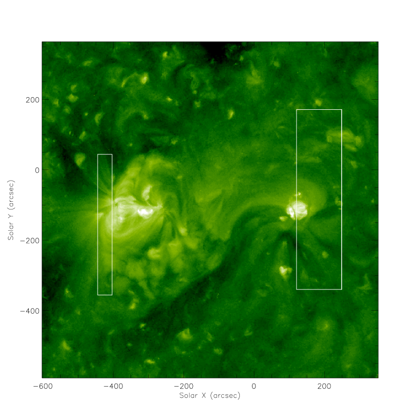
Figure 1: STEREO B/SECCHI EUVI observations of AR 10942 (on the left) and AR 10943 (on the right) taken at 195 Å on 2007 February 20 at 8:05. The Hinode/EIS FOV at 05:47–07:59 UT for AR 10943 and at 11:16-11:37 UT for AR 10942 for the data analyzed in this paper are drawn as rectangles.

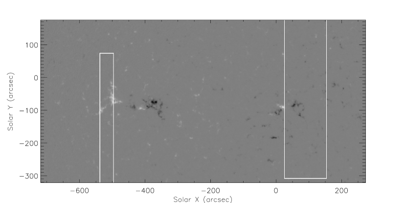
Figure 2: Full-disk SoHO/MDI magnetic field measurements on 2007 February 20 at $T_{ref}=8:05$ UT clipped to the area used for the magnetic field extrapolations. Both AR 10942 (left) and 10943 (right) are visible. The Hinode/EIS FOV (at 05:47–07:59 UT for AR 10943 and at 11:16-11:37 UT for AR 10942, see Sec. 2.2) are drawn as rectangles.

On 2007 February 20, less than four months after its launch, the heliocentric separation angle between the STEREO B probe and the Earth was still negligible ($0.1\,\deg$). This means that STEREO B/SECCHI EUVI images (Kaiser et al. 2008; Howard et al. 2008) have the same viewing angle than SoHO and Hinode and that we can use these images in combination with SoHO/MDI and Hinode/EIS. STEREO/SECCHI EUVI was in its normal mode, with full-disk observations at a cadence of 10 min in the EUV channel $\lambda$195Å. We selected the 8:05 UT observation corrected by EUVI_prep from the SolarSoft library, shown in Fig.1.

In this image, both active regions can be seen simultaneously. On the eastern side, the EUVI image in 195 Å displays the AR 10942 complex made of a set of loops connecting the two extreme polarities (see Fig. 2) of the AR, mainly in the southern side. Some straight (mostly fan-like) structures are also clearly seen on the north-eastern side (X = -400, Y = -50 to 0, see Fig. 1) which are candidate for open magnetic fields. At South, below AR 10942, internal loops, rather compact structures (X = -300, Y = -300) seem to be the feet of (apparently) very sheared loops. On the western side of the image, another smaller and compact AR (10943) does not seem to be connected with its neighbouring regions, except for a set of diffuse loops at the East of AR 10943 whose feet seem to be located in between the two ARs. One also notes that the lower side of these diffuse loops is very sharp. The overall picture is that the two ARs seem to be very disconnected on one hand, and that the eastern feet of the diffuse loops mentioned above could coincide with the QSL labelled “e” in Fig.4 of Baker et al. (2009), on the other hand. The EUVI image in the hot 284Å line confirms this picture, contrary to the He II image where the chromosphere between the two AR does not seem to be very perturbed. Finally, the 171 image is more puzzling because it does not display the above (too) hot loops but also shows some dark area on the western side of AR 10942, which could be a coronal hole or a filament channel.

2.2 Spectroscopic observations

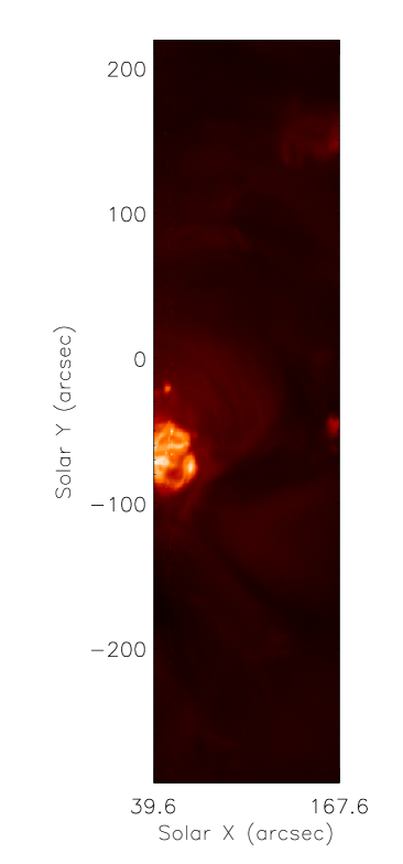
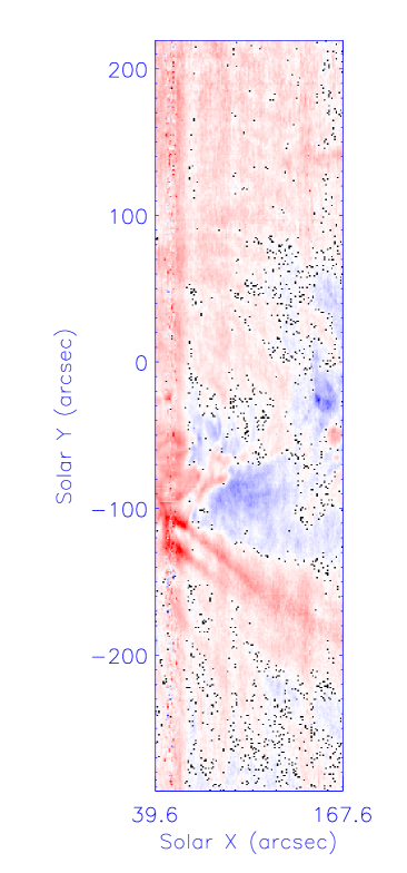
a) b)

c) d)

Figure 3: Maps of AR 10943 observed on 2007 February 20 at 05:47–07:59 UT with Hinode/EIS in Fe XII 195.12 Å: a) Intensity (integrated on the wavelength dimension); b) Centroid wavelength; c) density from the Fe XII 196.64 Å/ Fe XII 195.12 Å line ratio; d) Mass flow through a surface perpendicular to the line of sight.

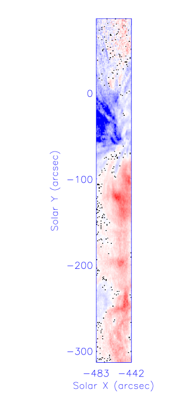
a) b)

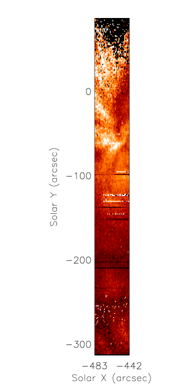
c) d)

Figure 4: Maps of AR 10942 observed on 2007 February 20 at 11:16-11:37 UT with Hinode/EIS in Fe XII 195.12 Å: a) Intensity (integrated on the wavelength dimension); b) Centroid wavelength; c) density from the Fe XII 196.64 Å/ Fe XII 195.12 Å line ratio; d) Mass flow through a surface perpendicular to the line of sight.

Figure 5: Density as a function of the Fe XII 196.64 Å/Fe XII 195.12 Å intensity ratio according to CHIANTI (Dere et al. 2009). The dashed lines represent the average of the intensity ratio and the corresponding density. The dotted lines represent the error bars on the intensity ratio computed from the uncertainties on the measurements of intensities and the related density error bars.

Spectroscopic information can be obtained from the Hinode/EUV imaging spectrometer (EIS; Culhane et al. 2007). We select two raster scans on 2007 February 20 that covers part of AR 10943 (at 05:47 UT, study ID 45) and part of AR 10942 (at 11:16 UT, study ID 57) respectively in order to have full spectra (around selected spectral lines) as a function of both solar dimensions in this region. The slit positions during these raster scans are shown in the STEREO image (Fig. 1) and in Table 1. Both raster scans are partial on the active regions. Nevertheless, as we show with magnetic field extrapolation in Sec 3, the feet of the interconnecting loops between the two active regions are located at the respective edges of the active regions in the FOV of EIS. So the raster scans are sufficient for our study. The delay of the scans and between the scans are negligible in comparison with the time of the continuous flows which are visible on a few days.

We apply the correction procedures eis_prep and eis_slit_tilt from the SolarSoft library. An additional correction must be applied for the orbital temperature variation of EIS; for this we have chosen to develop a specific method which is described in Appendix A : we use the orbital variation in the He II 256.32 Å line to correct the orbital lineshifts in other lines. Indeed, this line is chromospheric and optically thick, the insensitivity of its centroid with respect to activity allows us to better isolate orbital variations.

We focus on the Fe XII 195.12 Å line which is emitted around $\log T=6.1$. We produce intensity (Fig. 3a for AR 10943 and Fig. 4a for AR 10942) and Doppler velocity (Fig. 3b for AR 10943 and Fig. 4b for AR 10942) maps deduced from the parameters of a single Gaussian fit of this line using the correction of orbital variation. We choose to ignore the self-blending of Fe XII 195.12 Å  with Fe XII 195.18 Å because we do not focus on the width (which is the most influenced parameter) and our study concerns low density structures where the contribution of Fe XII 195.18 Å is negligible (Young et al. 2009).

The level 2 data show that the velocities in the active region are of the same order in the other EIS windows available except for Fe XIII 196.54 Å where that pattern is reversed. In the Fe XII 186.88 Å and Ca XVII 192.82 Å lines, the core of the AR is blue but the other structures are the same. We cannot conclude about the Fe XIII 196.54 Å and Fe XII 186.88 Å lines velocities because they are far different from the Fe XIII 202.04 Å and Fe XII 195.12 Å respectively. The automatic analysis could not be sufficient. The Ca XVII 192.82 Å line shows that the flow is upward in the core of the AR at very high temperature ($\log T_{max}=6.7$) but there are still downflows in the vicinity of the active region.

However the flow rate through a surface perpendicular to the line-of-sight is higher there than in the rest of the whirl. These downflows are persistent for a few days, therefore an impulsive event such as a jet is excluded as a viable mechanism producing these localised redshifts.

One also notes a redshifted area in the top third of the raster FOV. This area is not studied here for two reasons: it is not magnetically connected to AR 10942 (see Sec. 3.2) and the redshift is rather weak (a few km.s^-1).

We get a density map (Fig. 3c for AR 10943 and Fig. 4c for AR 10942) by also fitting the Fe XII 196.64 Å line, and computing the Fe XII 196.64 Å/ Fe XII 195.12 Å intensity ratio, which is sensitive to density. The density is deduced from the theoretical intensity ratio produced by the CHIANTI atomic database (Dere et al. 1997, 2009), as shown in Fig. 5.

In order to derive the flow rate through a surface perpendicular to the line-of-sight (Fig. 3d for AR 10943 and Fig. 4d for AR 10942), we multiply the density by the Doppler velocity.

The core of AR 10943 is characterized by hot loops bright in intensity (with a maximum of 9500 counts/pix, Fig. 3a), downward Doppler velocities and high densities between $4\times 10^{9}$ cm^-3 and $1\times 10^{10}$ cm^-3. These densities are consistent with values in active region loops by Warren et al. (2008) ($1.3\times 10^{9}$ and $9.5\times 10^{10}$ cm^-3 for Fe XII) and with Young et al. (2009) ($3\times 10^{8}$ cm^-3 $\leq n_{e}\leq$ $1\times 10^{11}$ cm^-3). The whirl of faint plasma around the core of AR 10943 is mostly blueshifted, with electron density between $6.3\times 10^{8}$ and $1\times 10^{9}$ cm^-3; moreover there is a clear straight redshifted (up to 16 km.s^-1) structure cutting the whirl in the South-East edge where the density is notably low (around $5\times 10^{8}$ cm^-3) but higher than Quiet Sun densities for Fe XII ($n_{e}=2.5-3.2\times 10^{8}$ cm^-3, Warren & Brooks 2009).

3 Magnetic connection between AR 10943 and AR 10942

3.1 Magnetic field observations

We investigate the possible magnetic connectivity between the two active regions AR 10942 and AR 10943. We use a SOHO/MDI level 1.8 96 minutes line-of-sight magnetogram (see Fig.2) to study the distribution of the photospheric magnetic field. The SOHO/MDI magnetograms have been recorded on 2007 February 20 at $T_{ref}=08:05$ UT (between the raster scans analysed in Sec. 2 and simultaneous with the STEREO SECCHI/EUVI image of fig. 1). We select an area encompassing the active regions (heliocentric coordinate $x$ from -720 to 275 arcsec and $y$ from -321 to 177 arcsec). The total unsigned magnetic flux for this area is $4.05\times 10^{22}$ Mx and the flux unbalance is only about 1.7% (a very low value for extrapolation). The total unsigned flux for AR 10942 is $9.90\times 10^{21}$ Mx with a negative flux of $4.44\times 10^{21}$ Mx and a positive flux of $5.46\times 10^{21}$ Mx. For AR 10943, the total unsigned flux is $5.53\times 10^{21}$ Mx with a negative flux of $4.12\times 10^{21}$ Mx and a positive flux of $1.41\times 10^{21}$ Mx. The net magnetic flux for AR 10943 is about 50% of the total flux. AR 10943 is in excess of negative flux, while AR 10942 is in excess of positive flux. If a magnetic connection exists between the two active regions, thus this connection is between the positive polarity of AR 10942 and the negative polarity of AR 10943.

3.2 Magnetic field extrapolation

(a)

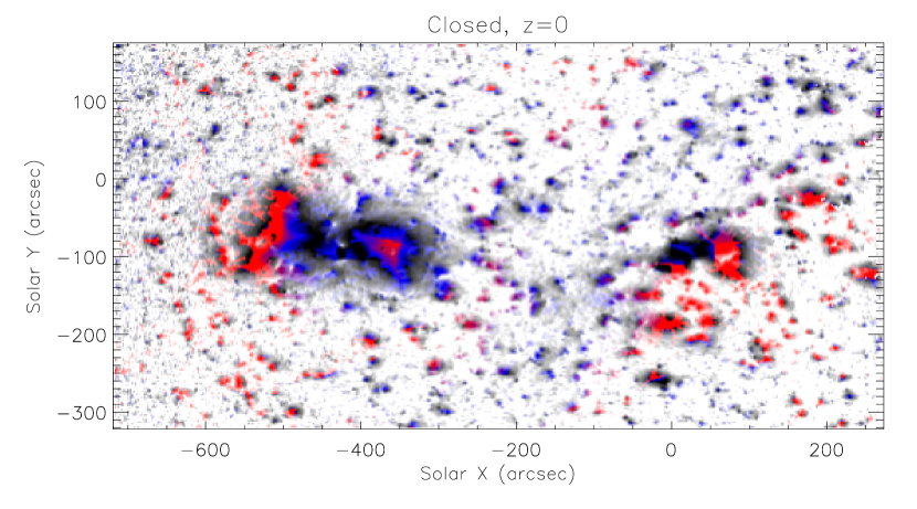
(b)

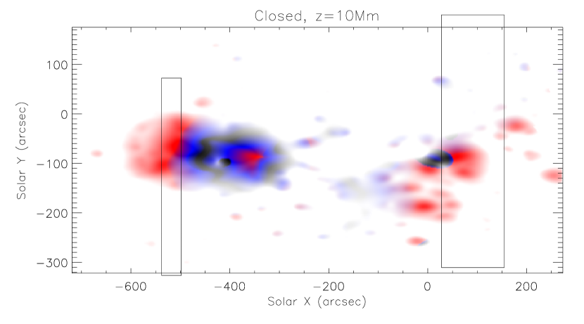
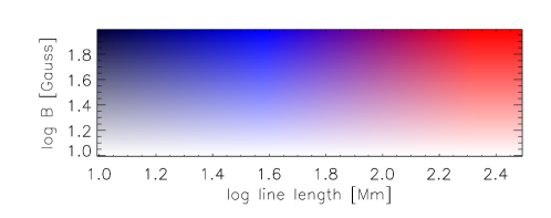
(c) (c)

Figure 6: Connectivity maps for the potential field model in the case of closed boundary conditions, at two different altitudes: at the photosphere $z=0$ (a) and at $z=10$Mm (b). The color in any given pixel represents the length of the closed magnetic field line starting from this point (at the given altitude) and the modulus of the magnetic field at this position, according to the caption in panel (c). The magnetic field is color-coded from 10 to 100 G and saturated below and above these values, while the the length is coded from 10 to 300 Mm and saturated below and above these values. Rectangles in (b) indicate the EIS FOV.

To study the connectivity between the two active regions, we derive the 3D magnetic field based on a potential field extrapolation (e.g., Schmidt 1964; Semel & Rayrole 1968). The potential field assumption cannot describe the effects of electric current on the magnetic field lines such as shear arcades or twisted flux bundles. However, the potential field assumption is a good estimation of the large-scale connectivity of the magnetic field (see.g., Schatten et al. 1969; Levine 1982; Wang & Sheeley 1992). In addition, Régnier (2011) showed that, by comparing several magnetic field assumptions (potential, linear force-free, and nonlinear force-free fields), the magnetic topology and connectivity are well preserved when the current density is modified, which justifies the use of the potential model in this study.

The potential field extrapolation method solves the following equation:

$$\vec{\nabla}\times\vec{B}=\vec{0},$$ (1)

with the bottom (or photospheric) boundary condition given by the vertical component of the magnetic field provided by the SOHO/MDI magnetogram selected area (see Sec. 3.1). The numerical technique relies on the computation of the scalar potential associated to the magnetic field satisfying the Laplace equation. We perform the potential field extrapolation for closed boundary conditions for which the normal component of the magnetic field vanishes on the sides and top boundaries. For the use of the SOHO/MDI magnetogram as boundary conditions, we need to put constraints:

• the center of the FOV is near the disk center and the active regions are in a range of longitudes between E30 and W10, therefore the line-of-sight magnetic field is not subject to projection effects;

• the line-of-sight magnetic field component $B_{s}$ is converted into the vertical (radial) component $B_{z}=B_{s}/\cos\theta$ where $\theta$ is the angle between the line-of-sight and the normal to the surface.

• as the magnetic field component satisfies the two items above, we assume that the curvature of the Sun does not affect the connectivity of the field. We thus compute the potential field in Cartesian coordinates.

• as the magnetic flux through the surface containing the two active regions is nearly balanced ($<$2%), we do not force the magnetic flux to be strictly balanced.

In Fig. 6, we plot the connectivity maps for the potential model with closed boundary conditions: each pixel is color-coded as a function of the length of the field line associated with the photospheric footpoint and as a function of the magnitude of the field, according to the caption in panel (c). The connectivity maps have been computed at two different altitudes: at the photosphere $z=0$ (a) and at $z=10$ Mm (b). The modulus of the magnetic field is below 10 G in the Quiet Sun, mostly between 10 G and 100 G in the active regions at 10 Mm while superior to 100 G in some active areas at $z=0$. Long field lines linking the two active regions definitely exist, when starting from both altitudes. At the photospheric level, we notice that the connectivities have various sizes and magnitudes, the smallest (and faintest) ones corresponding to local dipoles in the quiet Sun. On the contrary, at $z=10$ Mm, these local dipoles disappear, probably because of their small size, and consequently altitude. One recognizes the essential long range connectivity between the two AR, along with an internal connectivity within AR 10942. This large scale connectivity between the two AR has already been found using different models by Sakao et al. (2007), who did not discuss it, and by Harra et al. (2008).

3.3 Estimation of the mass flows

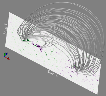
(a)
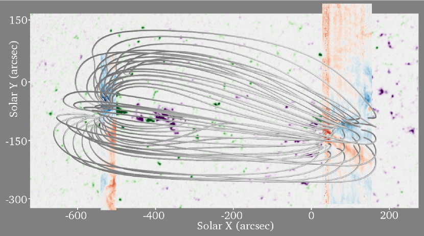
(b) (c)

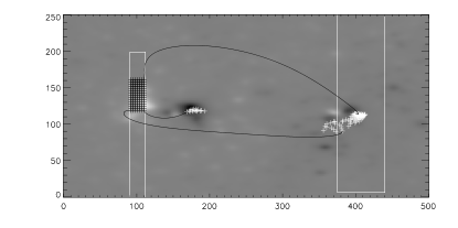
Figure 7: Some selected magnetic field lines from a potential magnetic field extrapolation, with the MDI image as background: (a) Viewed from above with superimposition of the velocity maps from EIS for AR 10942 and AR 10943; (b) Viewed from a point of view in the Southern hemisphere; (c) Start (black crosses) and end (white crosses) points of the field lines used in Sec. 3.3 on a map of $B_{z}$ at the 10 Mm altitude obtained from the extrapolation; three selected lines are drawn in black. The black frames are the EIS FOV.

We explore further the magnetic field connection between the ARs, using the potential field extrapolation (Fig. 7a and b) and EIS spectral scans. The co-alignement between maps of EIS intensity and maps of the extrapolated magnetic field is made by using cross-correlation between MDI (8:05 UT) and STEREO Fe XII 195 (8:05 UT) image and cross-correlation between STEREO Fe XII 195 image and EIS Fe XII 195.12 (respectively at 05:47 UT for AR 10943 and at 11:16 UT for AR 10942).

For each AR, we have measurements of the line-of-sight velocity $v_{s}$ (oriented downwards), and the signed mass flux through a surface $S$ orthogonal to the line-of-sight is

$$F=\iint_{S}\rho\vec{v}\cdot d^{2}\vec{S}$$ (2)

which reduces to $\rho v_{s}S$ if $S$ is small enough. Note that $F$ has the same sign as $v_{s}$.

We choose to consider the two sections $S_{1}$ and $S_{2}$ of the flux tube represented in Fig. 8. We decompose $S_{1}$ into small areas $S_{1i}$ and then we define $S_{2i}$ by the intersection with $S_{2}$ of the flux tube originating from $S_{1i}$: we have $S_{1}=\sum_{i}S_{1i}$ and $S_{2}=\sum_{i}S_{2i}$.

The ratio of the total mass flux through $S_{2}$ to the total mass flux through $S_{1}$ is

$$R=\frac{F_{2}}{F_{1}}=\frac{\sum_{i}F_{2i}}{\sum_{i}F_{1i}}=\frac{\sum_{i}\rho_{2i}v_{s2i}S_{2i}}{\sum_{i}\rho_{1i}v_{s1i}S_{1i}}$$ (3)

We use the conservation of the magnetic flux $\phi_{i}$ in each of these small flux tubes:

$$|\phi_{i}|=|B_{s1i}|S_{1i}=|B_{s2i}|S_{2i}$$ (4)

and we decompose $S_{2i}$ into $S_{1i}S_{2i}/S_{1i}$, which gives $S_{2i}=S_{1i}|B_{s1i}/B_{s2i}|$. Finally, as all $S_{1i}$ are chosen with the same area (a MDI pixel), we obtain the mass flux ratio

$$R=\frac{\sum_{i}\rho_{2i}v_{s2i}|B_{s1i}/B_{s2i}|}{\sum_{i}\rho_{1i}v_{s1i}}$$ (5)

In this equation, the density and the Doppler velocity from the EIS Fe XII spectra in AR 10942 and 10943 (see Sec. 2.2) are derived with a $3\times 3$-pixel median filter. We consider that the Fe XII lines are emitted at an altitude of 10 Mm in hot loops. The values of the line-of-sight magnetic fields $B_{1i}$ and $B_{2i}$ are taken from the footpoints of magnetic field lines starting at an altitude of 10 Mm on a $7\times 15$-point grid in the outflow at the edge of AR 10942 (Fig. 7c), and computed until they reach again the same altitude of 10 Mm. 76 among 105 of these lines link AR 10942 and AR 10943 and fall inside the EIS FOV on AR 10943.

We consider these lines to be representative of the flux tubes connecting AR 10942 to AR 10943. The modulus of the mass flux ratio (AR 10943 over 10942, see Eq. 3) is then 0.18.

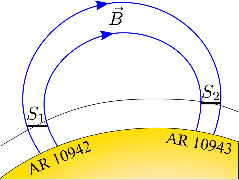
Figure 8: Cartoon of the magnetic flux tube connecting AR 10942 and AR 10943. $S_{1}$ and $S_{2}$ are the cross-sections perpendicular to the line-of-sight of the flux tube at the observed altitude (we chose 10 Mm for Fe XII), above AR 10942 and AR 10943 respectively. The magnetic field in cross-section $S_{i}$ is $\vec{B}_{i}$, the density is $\rho_{i}$, and the velocity is $\vec{v}_{i}$.

We compute the uncertainty on the mass flux ratio induced by the uncertainties on the observations by

$$\frac{\delta R}{R}=\frac{\delta F_{1}}{|F_{1}|}+\frac{\delta F_{2}}{|F_{2}|}$$ (6)

with

$$\frac{\delta F_{1}}{|F_{1}|} =\frac{\frac{1}{\sqrt{n}}\sum_{i}|F_{1i}|\frac{\delta F_{1i}}{|F_{1i}|}}{|F_{1}|}$$

$$=\frac{1}{|F_{1}|\sqrt{n}}\sum_{i}|v_{s1i}|\rho_{1i}\left(\frac{\delta\rho_{1i}}{\rho_{1i}}+\frac{\delta v_{s1i}}{|v_{s1i}|}\right)$$ (7)

and

$$\frac{\delta F_{2}}{|F_{2}|} =\frac{\frac{1}{\sqrt{n}}\sum_{i}|F_{2i}|\frac{\delta F_{2i}}{|F_{2i}|}}{|F_{2}|}$$

$$=\frac{1}{|F_{2}|\sqrt{n}}\sum_{i}\rho_{2i}|v_{s2i}B_{s1i}/B_{s2i}|\times$$ (8)

$$\qquad\left(\frac{\delta\rho_{2i}}{\rho_{2i}}+\frac{\delta v_{s2i}}{|v_{s2i}|}+\frac{\delta B_{s1i}}{|B_{s1i}|}+\frac{\delta B_{s2i}}{|B_{s2i}|}\right).$$

We have chosen a uniform $\delta v$ of $2$ km.s^-1 as we have an uncertainty of about $\pm 1$ km.s^-1 for the Doppler velocity from each line fit, $\delta\rho=3.4\times 10^{8}$ cm^-3 from the uncertainties on the intensities of the lines used to deduce the density (Fig.5), and $\delta B=10$ G, a value below which coherent small-scale patterns disappear in the quiet Sun. The relative uncertainty $\delta R/R$ on the mass flux ratio is then found to be 0.30.

To evaluate the uncertainty due to the co-alignment between MDI data and EIS spectra, we compute the mass flux ratio with a co-alignment shifted by one MDI pixel (1.98 arcsec) in the two X and Y directions with respect to EIS data. The mass ratios obtained vary by a factor 2. We can then state that the co-alignment is the main cause of uncertainty.

4 Discussion

The extrapolation clearly shows us how AR 10942 and AR 10943 are linked. From the observation of both ARs, it appears that the mass flow to AR 10943 seems to be 18% of the upflows from AR 10942. We can therefore conclude that the flow leaving the Sun among the upflows from AR 10942 is at most 82% of the measured upflows. Some of these upflows could be confined somewhere else.

Another solution is not explored by our extrapolation: the presence of a Y point between the two ARs. An argument in favour of this hypothesis is the difference between the velocities at the AR 10942 edge and the AR 10943 edge. Indeed, in the model proposed by Del Zanna et al. (2011), the velocity is higher for the strongest magnetic bipoles than in the faintest pole (a Coronal Hole in their model). In this case, the flows are not directly linked and they interact with each other through an X point. In our case we clearly have open field lines, with the presence of two coronal holes, one located at the Eastern part of AR 10942 and — with less evidence — the other one in the Western part of AR 10943, which then would lead to a high-altitude Y point (Fig. 9). As a consequence, the measured upflows in the Eastern part include flows of material which escapes towards the Y point and the corona and cannot be found at the foot of the connecting loop in AR 10943. It is clear that the potential extrapolation does not allow to explore this possibility.

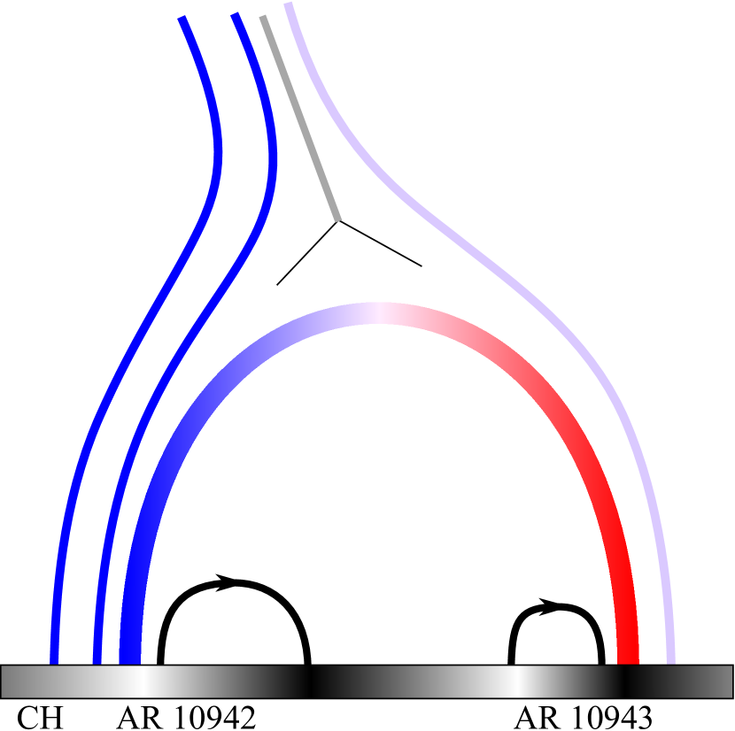
Figure 9: Cartoon of the magnetic field and flows in the case of a Y point. The colors of the lines show the Doppler shifts that would be observed from above, with the usual convention: blue for upflows and red for downflows. The Y point is located above the colored loop and is shown with the current sheet in grey. Some field lines are indicated with arrows. At the bottom, the magnetic polarities coded in the usual white and black convention correspond to the location of the two ARs and the eastern coronal hole.

5 Conclusion

In summary, we observed Doppler-shifted structures at the edges of two Active Regions which we find to be connected with each other by large scale loops, a result we discuss in more details below. With the advent of the EUV spectrometer EIS on Hinode, special attention has been paid on high temperature flows around coronal holes and active regions. AR 10942 has been extensively studied (e.g. Baker et al. 2009) and it has been suggested that the strong observed upflow at its boundary could be one of the sources of the solar wind. In order to properly assess this critical result, we have investigated the possibility that the supposedly open field in this area could be actually (at least partially) connected to the preceding AR 10943 with the consequence that part of the mass outflow from AR 10942 could turn into downflow in AR 10943. In order to investigate this possibility, we analyzed the EIS spectra obtained in AR 10943 with special attention to the Fe XII (195 Å) line formed at $\log T=6.1$.

The EIS spectra are difficult to analyze for two reasons: most lines are blended and their profiles are affected by a strong (presumably thermal-induced) deformation during any orbit. The blends are properly dealt with the use of multi-gaussian fits. As far as the second (orbital) correction is concerned, the EIS software allows to take into account the relative shift of the profile over the orbit but leaves open the issue of the absolute reference. In order to overcome this difficulty, we have designed and used a technique which relies upon the cool and optically thick 256 Å He II line, consequently less sensitive to activity and induced flows. The technique is described in Appendix A.

The analysis of the velocity field in AR 10943, performed with this technique, shows a significant feature located in the southwestern part where the downflow velocity reaches 16 km.s^-1. It should be pointed out again that this pattern is confirmed in other lines, as mentioned in Sect. 2.2, with the noticeable exception of the Fe XIII line at 196.5 Å which is a very weak line (Young et al. 2009). At very high temperature (Ca XVII 192.82 Å), it seems that the pattern is the same except for the core of the active region which is blueshifted. Moreover, through the use of the two Fe XII lines (196.6 Å and 195.1 Å) and their intensity ratio, we were able to build a density map where the downflow region density reaches a value of $5.10^{8}$ cm^-3.

We then proceeded to establish the connectivity between the two regions, and especially between the blueshifted area of AR 10942 and the redshifted area of AR 10943. A potential extrapolation, rather suitable for our stable active regions, was used. The connectivity between the two areas was well established although the computed field lines do not clearly appear as inter-connecting loops in the Fe XII image (Fig. 1), presumably a result of their low densities. With the values of the local density and line-of-sight velocity in the two areas, we could compute and compare the mass flows between the respective feet of the magnetic field lines. We concluded that only 18% of the outgoing flow from AR 10942 is retrieved as downward flow in AR 10943, as computed along the extrapolated field lines. We elaborated upon the possibility of other paths followed by the upflows of AR 10942, for various reasons: one of them being the presence of open fields in AR 10942, which our extrapolation does not take into account; another one being the possibility of a breach of connectivity due, e.g. to a Y point where reconnection occurs (Del Zanna et al. 2011).

As a conclusion, we can state that some material is exchanged between the two active regions, especially from the area of the upflow but that 82% of the upflow from AR 10942 is missing upon arrival on AR 10943. Actually, these flows could be a condition for the thermal sustainability of such long loops during such a long time span. However, we cannot go further because of the many factors and uncertainties involved in the observations, whether the wavelength (velocity) reference, the non-simultaneity of the two AR observations with EIS, the reduced fields of view, or even the validity of the potential field extrapolation.

We strongly recommend that further similar studies rely upon force-free magnetic field extrapolation made possible by simultaneous SOT/Hinode observations and also closer-in-time observing modes focused on the active regions involved. We also suggest to use the reference wavelength method described in the Annex.

Appendix A Wavelength reference for EIS

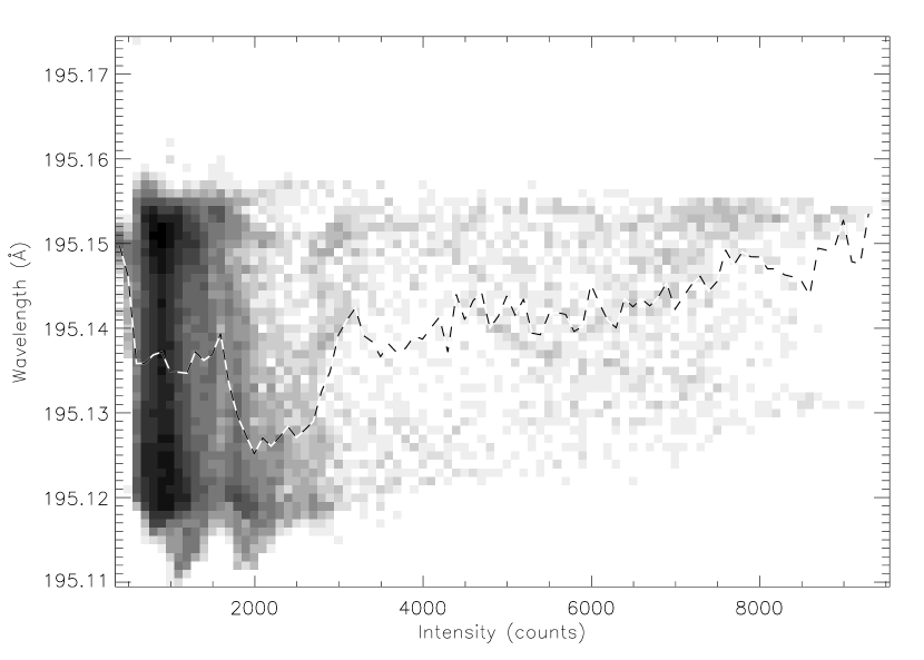
Figure 10: Dispersion of the centroid wavelength of the Fe XII line profile depending on the intensity (counts) before the orbital correction.

The temperature variation along the orbit of Hinode deforms the optical axis of EIS in the dispersion plane (Brown et al. 2007). The determination of the Doppler velocity is therefore more difficult because of the lack of absolute reference. Figure 10 shows the wide range (0.05  Å) of the Fe XII wavelengths given by EIS before any correction. Therefore a correction is necessary. It has been observed (Brown et al. 2007) that this orbital variation of the wavelength is not the same from one orbit to the other and depends on several parameters (Hinode pointing, Earth’s seasons, etc.). Thus, it is not predictable and the orbital correction, based on the considered science data set, has to be empirical, although a correction where housekeeping data are used (Kamio et al. 2010) is possible. Nevertheless, as the orbital variation is the same for both detectors, we can use the observation of any line to correct the others (Mariska et al. 2007).

The measured wavelength depends on the physical parameters on the Sun and the instrumental bias including the orbital variation. We want to separate these two components of the wavelength line centroid. We assume that the Doppler shifts are globally null on average in the Y dimension while the orbital variation is the same on each pixel along the Y dimension of the slit at a given time. So we can isolate the orbital variation by integrating on the Y axis. In order to smooth any residual Doppler shifts, we use a spline depending on time.

The procedure consists in averaging the line profiles along the Y axis in the quiet Sun pixels and then to fit these integrated lines with a Gaussian in order to obtain the mean wavelength of the line centroid depending on the time $\lambda_{av}(t)$. The line centroids $\lambda_{av}(t)$ obtained are fitted with a spline $\mathcal{S}(t)$) in order to keep only the orbital variation. The correction, that is to say the difference between the spline and the reference wavelength $\lambda_{0}$ (as given in CHIANTI), is denoted $\delta\lambda(t)$.

The usual way of finding the wavelength reference consists in following the above procedure. However, the issue of the line shift in the corona is not solved today. From SUMER/SOHO, it was derived that the redshift observed in the transition region (with a maximum of 30 km.s^-1 at logT= 5.3) decreased at high coronal temperatures but remained a redshift (e.g. Chae et al. 1998). Then also with SUMER data, Peter & Judge (1999) showed that at high temperatures, one actually had a blueshift, i.e. upward velocities. Consequently, we suspect that taking a hot line as a wavelength reference, even with a substantial spatial averaging, may not be a safe procedure.

As the He II 256.32 Å line is the coldest line in the EIS wavelength ranges (being formed from the upper chromosphere to the lower transition region) and is optically thick, the line is less affected by the solar flows than the other EIS lines. Therefore, the centroid of its profile is an efficient reference. The drawback is that He II 256.32 Å is blended with hot lines. In the quiet Sun, He II 256.32 Å is dominant (its contribution is more than 80% of the blend (Young et al. 2007) and can be separated from the blending lines with a two-Gaussian fit. For the active Sun, it is more difficult to separate He II 256.32 Å from its blends, as they are hot lines and their contribution is changing depending on the observed structures.

In our study, for example, we choose to apply the correction obtained from He II 256.32 Å on the Fe XII 196.64 Å line. We computed $\delta\lambda_{HeII}(t)$, we fitted $\lambda_{FeXII}(y,t)$ by a gaussian fit and we corrected each pixel following the formula $\lambda_{FeXIIcorrected}(y,t)=\lambda_{FeXII}(y,t)-\delta\lambda_{HeII}(t)$

As He II 256.32 Å is essentially blended with Si X 256.37 Å (Del Zanna & Mason 2005). We consider that we can fit these two lines only. Because Si X 261.04 Å and Si X 256.37 Å have the same lower level ($2s2p^{2\>2}P_{1/2}$), we can use the branching ratio between Si X 261.04 Å and Si X 256.37 Å in order to evaluate the contribution of Si X 256.37 Å in the 256 Å blend. The branching ratio denoted $\alpha$ is determined by the ratio of the intensities given by CHIANTI.

The procedure is as follows :

• At first, we fit Si X 261.04 Å with a simple Gaussian. We obtain $\lambda_{Si\,X261}$, $I_{Si\,X261}$,$FWHM_{Si\,X261}$ and the background.

• We transpose the characteristics we obtained for Si X 261.04 Å to Si X 256.37 Å, that is to say for the wavelength, $\lambda_{Si\,X256}=\lambda_{Si\,X261}-\lambda_{0,Si\,X261}+\lambda_{0,Si\,X256}$, we consider the same width, and for the intensity, $I_{256}=\alpha I_{261}$ where $\alpha$ is the branching ratio.

• We fit He II 256.32 Å and its blend with a 5-parameter fit ($\lambda_{He\,II}$, $I_{He\,II}$, $I_{Si\,X256}$, $FWHM_{He\,II}$ and the intensity background), with fixed value for $\lambda_{Si\,X256}$ and $FWHM_{Si\,X256}$.

• We extract the correction $\delta\lambda(t)$ from $\lambda_{He\,II}(t)$ as described previously and subtract it from the wavelength obtained for the studied line.

Figure 11 shows the dispersion of the wavelength of Fe XII 195.12 Å after the correction proposed in this appendix. We can note that the wavelength increases slightly with the intensity, a result in agreement with the fact that the Active Region is slightly redshifted. The orbital correction computed with the SolarSoft library based on the Fe XII 195.12 Å line shows the same tendency (Fig.12). There is a systematic difference of 0.008 Å between the two corrections which is consistent with the line shift depending on the temperature discussed in Chae et al. (1998) and in Peter & Judge (1999). They reported a redshift of 5.3 km.s^-1 for Si III $\lambda$ 1206.51+$\lambda$ 1206.53 Å  (Chae et al. 1998) at about the same temperature as He II 256 ($\log T_{max}=4.7$) and a blueshift of 6 km.s^-1 for Fe XII 1349 Å line (Sandlin et al. 1977) which corresponds to a total relative Doppler shift of 0.008 Å. Therefore, we apply a redshift of 0.008 Å on our Doppler shifts analysis (Sec. 2.2 and Sec. 3.3), which implies that we adopt an average quiet Sun Fe XII line line at rest.

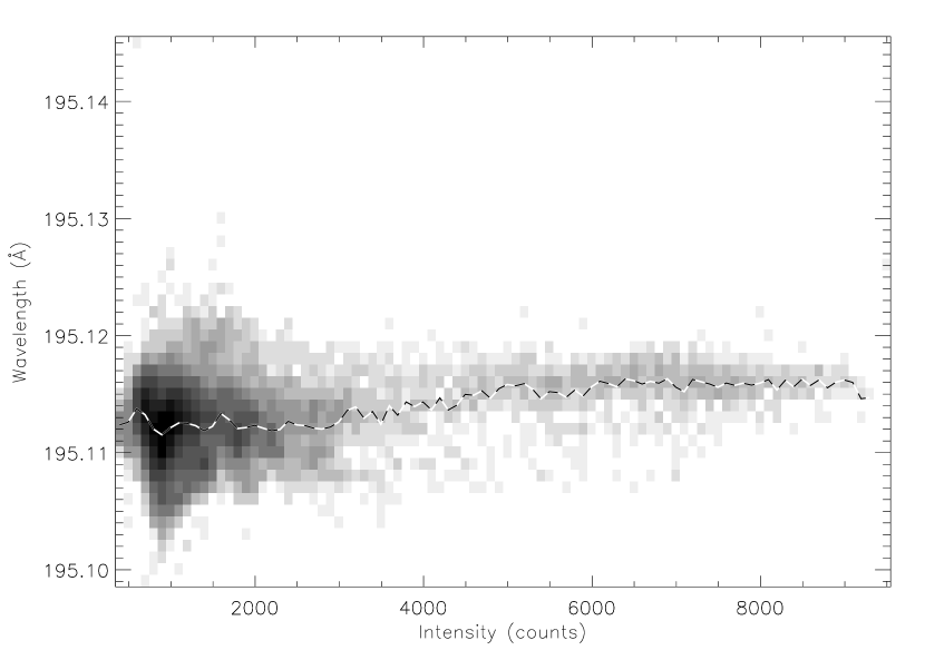
Figure 11: Dispersion of the centroid wavelength of the Fe XII line profile depending on the intensity (counts) after the orbital correction using He II.

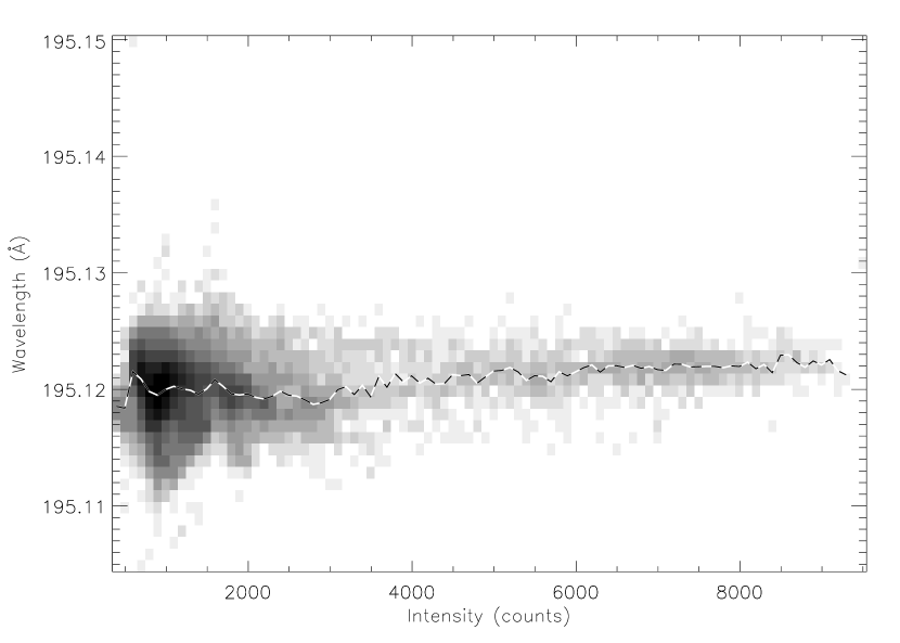
Figure 12: Dispersion of the centroid wavelength of the Fe XII line profile depending on the intensity (counts) after the orbital correction using Fe XII.

References

- Abbo et al. (2010) Abbo, L., Antonucci, E., Mikić, Z., Linker, J. A., Riley, P., & Lionello, R. 2010, Advances in Space Research, 46, 1400
- Baker et al. (2009) Baker, D., van Driel-Gesztelyi, L., Mandrini, C. H., Démoulin, P., & Murray, M. J. 2009, ApJ, 705, 926
- Brosius (2006) Brosius, J. W. 2006, ApJ, 636, L57
- Brown et al. (2007) Brown, C. M., Hara, H., Kamio, S., Feldman, U., Seely, J. F., Doschek, G. A., Mariska, J. T., Korendyke, C. M., Lang, J., Dere, K. P., Culhane, L., Thomas, R. J., & Davila, J. M. 2007, PASJ, 59, 865
- Chae et al. (1998) Chae, J., Yun, H. S., & Poland, A. I. 1998, ApJS, 114, 151
- Culhane et al. (2007) Culhane, J. L., Harra, L. K., James, A. M., Al-Janabi, K., Bradley, L. J., Chaudry, R. A., Rees, K., Tandy, J. A., Thomas, P., Whillock, M. C. R., Winter, B., Doschek, G. A., Korendyke, C. M., Brown, C. M., Myers, S., Mariska, J., Seely, J., Lang, J., Kent, B. J., Shaughnessy, B. M., Young, P. R., Simnett, G. M., Castelli, C. M., Mahmoud, S., Mapson-Menard, H., Probyn, B. J., Thomas, R. J., Davila, J., Dere, K., Windt, D., Shea, J., Hagood, R., Moye, R., Hara, H., Watanabe, T., Matsuzaki, K., Kosugi, T., Hansteen, V., & Wikstol, Ø. 2007, Sol. Phys., 243, 19
- Dadashi et al. (2011) Dadashi, N., Teriaca, L., & Solanki, S. K. 2011, A&A, 534, A90
- Del Zanna (2008) Del Zanna, G. 2008, A&A, 481, L49
- Del Zanna et al. (2011) Del Zanna, G., Aulanier, G., Klein, K.-L., & Török, T. 2011, A&A, 526, A137+
- Del Zanna & Mason (2005) Del Zanna, G. & Mason, H. E. 2005, Advances in Space Research, 36, 1503
- Dere et al. (1997) Dere, K. P., Landi, E., Mason, H. E., Monsignori Fossi, B. C., & Young, P. R. 1997, A&AS, 125, 149
- Dere et al. (2009) Dere, K. P., Landi, E., Young, P. R., Del Zanna, G., Landini, M., & Mason, H. E. 2009, A&A, 498, 915
- Doschek et al. (2007) Doschek, G. A., Mariska, J. T., Warren, H. P., Brown, C. M., Culhane, J. L., Hara, H., Watanabe, T., Young, P. R., & Mason, H. E. 2007, ApJ, 667, L109
- Fárník et al. (1999) Fárník, F., Karlický, M., & Švestka, Z. 1999, Sol. Phys., 187, 33
- Fárník et al. (2001) —. 2001, Sol. Phys., 202, 81
- Harra et al. (2008) Harra, L. K., Sakao, T., Mandrini, C. H., Hara, H., Imada, S., Young, P. R., van Driel-Gesztelyi, L., & Baker, D. 2008, ApJ, 676, L147
- Hassler et al. (1999) Hassler, D. M., Dammasch, I. E., Lemaire, P., Brekke, P., Curdt, W., Mason, H. E., Vial, J.-C., & Wilhelm, K. 1999, Science, 283, 810
- Howard et al. (2008) Howard, R. A., Moses, J. D., Vourlidas, A., Newmark, J. S., Socker, D. G., Plunkett, S. P., Korendyke, C. M., Cook, J. W., Hurley, A., Davila, J. M., Thompson, W. T., St Cyr, O. C., Mentzell, E., Mehalick, K., Lemen, J. R., Wuelser, J. P., Duncan, D. W., Tarbell, T. D., Wolfson, C. J., Moore, A., Harrison, R. A., Waltham, N. R., Lang, J., Davis, C. J., Eyles, C. J., Mapson-Menard, H., Simnett, G. M., Halain, J. P., Defise, J. M., Mazy, E., Rochus, P., Mercier, R., Ravet, M. F., Delmotte, F., Auchere, F., Delaboudiniere, J. P., Bothmer, V., Deutsch, W., Wang, D., Rich, N., Cooper, S., Stephens, V., Maahs, G., Baugh, R., McMullin, D., & Carter, T. 2008, Space Sci. Rev., 136, 67
- Kaiser et al. (2008) Kaiser, M. L., Kucera, T. A., Davila, J. M., St. Cyr, O. C., Guhathakurta, M., & Christian, E. 2008, Space Sci. Rev., 136, 5
- Kamio et al. (2010) Kamio, S., Hara, H., Watanabe, T., Fredvik, T., & Hansteen, V. H. 2010, Sol. Phys., 266, 209
- Kilpua et al. (2009) Kilpua, E. K. J., Luhmann, J. G., Gosling, J., Li, Y., Elliott, H., Russell, C. T., Jian, L., Galvin, A. B., Larson, D., Schroeder, P., Simunac, K., & Petrie, G. 2009, Sol. Phys., 256, 327
- Ko et al. (2006) Ko, Y.-K., Raymond, J. C., Zurbuchen, T. H., Riley, P., Raines, J. M., & Strachan, L. 2006, ApJ, 646, 1275
- Kojima et al. (1999) Kojima, M., Fujiki, K., Ohmi, T., Tokumaru, M., Yokobe, A., & Hakamada, K. 1999, J. Geophys. Res., 104, 16993
- Krieger et al. (1973) Krieger, A. S., Timothy, A. F., & Roelof, E. C. 1973, Sol. Phys., 29, 505
- Levine (1982) Levine, R. H. 1982, Sol. Phys., 79, 203
- Liewer et al. (2004) Liewer, P. C., Neugebauer, M., & Zurbuchen, T. 2004, Sol. Phys., 223, 209
- Madjarska et al. (2004) Madjarska, M. S., Doyle, J. G., & van Driel-Gesztelyi, L. 2004, ApJ, 603, L57
- Mariska et al. (2007) Mariska, J. T., Warren, H. P., Ugarte-Urra, I., Brooks, D. H., Williams, D. R., & Hara, H. 2007, PASJ, 59, 713
- McIntosh & De Pontieu (2009) McIntosh, S. W. & De Pontieu, B. 2009, ApJ, 706, L80
- Peter & Judge (1999) Peter, H. & Judge, P. G. 1999, ApJ, 522, 1148
- Régnier (2011) Régnier, S. 2011, ArXiv e-prints
- Sakao et al. (2007) Sakao, T., Kano, R., Narukage, N., Kotoku, J., Bando, T., DeLuca, E. E., Lundquist, L. L., Tsuneta, S., Harra, L. K., Katsukawa, Y., Kubo, M., Hara, H., Matsuzaki, K., Shimojo, M., Bookbinder, J. A., Golub, L., Korreck, K. E., Su, Y., Shibasaki, K., Shimizu, T., & Nakatani, I. 2007, Science, 318, 1585
- Sandlin et al. (1977) Sandlin, G. D., Brueckner, G. E., & Tousey, R. 1977, ApJ, 214, 898
- Schatten et al. (1969) Schatten, K. H., Wilcox, J. M., & Ness, N. F. 1969, Sol. Phys., 6, 442
- Schmidt (1964) Schmidt, H. U. 1964, in The Physics of Solar Flares, ed. W. N. Hess, p.107
- Schrijver & Title (2011) Schrijver, C. J. & Title, A. M. 2011, Journal of Geophysical Research (Space Physics), 116, A04108
- Schwadron et al. (2005) Schwadron, N. A., McComas, D. J., Elliott, H. A., Gloeckler, G., Geiss, J., & von Steiger, R. 2005, in ESA Special Publication, Vol. 592, Solar Wind 11/SOHO 16, Connecting Sun and Heliosphere, ed. B. Fleck, T. H. Zurbuchen, & H. Lacoste, 645
- Semel & Rayrole (1968) Semel, M. & Rayrole, J. 1968, in IAU Symp. 35: Structure and Development of Solar Active Regions, ed. K. O. Kiepenheuer, p.134
- Sheeley et al. (1997) Sheeley, Jr., N. R., Wang, Y.-M., Hawley, S. H., Brueckner, G. E., Dere, K. P., Howard, R. A., Koomen, M. J., Korendyke, C. M., Michels, D. J., Paswaters, S. E., Socker, D. G., St. Cyr, O. C., Wang, D., Lamy, P. L., Llebaria, A., Schwenn, R., Simnett, G. M., Plunkett, S., & Biesecker, D. A. 1997, ApJ, 484, 472
- Subramanian et al. (2010) Subramanian, S., Madjarska, M. S., & Doyle, J. G. 2010, A&A, 516, A50
- Tripathi et al. (2009) Tripathi, D., Mason, H. E., Dwivedi, B. N., del Zanna, G., & Young, P. R. 2009, ApJ, 694, 1256
- Vaiana (1976) Vaiana, G. S. 1976, Royal Society of London Philosophical Transactions Series A, 281, 365
- Wang et al. (2007) Wang, J., Zhang, Y., Zhou, G., Harra, L. K., Williams, D. R., & Jiang, Y. 2007, Sol. Phys., 244, 75
- Wang & Sheeley (1992) Wang, Y.-M. & Sheeley, Jr., N. R. 1992, ApJ, 392, 310
- Wang & Sheeley (2004) —. 2004, ApJ, 612, 1196
- Warren & Brooks (2009) Warren, H. P. & Brooks, D. H. 2009, ApJ, 700, 762
- Warren et al. (2008) Warren, H. P., Ugarte-Urra, I., Doschek, G. A., Brooks, D. H., & Williams, D. R. 2008, ApJ, 686, L131
- Young et al. (2007) Young, P. R., Del Zanna, G., Mason, H. E., Dere, K. P., Landi, E., Landini, M., Doschek, G. A., Brown, C. M., Culhane, L., Harra, L. K., Watanabe, T., & Hara, H. 2007, PASJ, 59, 857
- Young et al. (2009) Young, P. R., Watanabe, T., Hara, H., & Mariska, J. T. 2009, A&A, 495, 587