Submillimeter Polarization of Galactic Clouds:
A Comparison of $350\,\micron$ and $850\,\micron$ Data

Abstract

The Hertz and SCUBA polarimeters, working at $350\,\micron$ and $850\,\micron$ respectively, have measured the polarized emission in scores of Galactic clouds. Of the clouds in each dataset, 17 were mapped by both instruments with good polarization signal-to-noise ratios. We present maps of each of these 17 clouds comparing the dual-wavelength polarization amplitudes and position angles at the same spatial locations. In total number of clouds compared, this is a four-fold increase over previous work. Across the entire data-set real position angle differences are seen between wavelengths. While the distribution of $\phi(850)-\phi(350)$ is centered near zero (near-equal angles), 64% of data points with high polarization signal-to-noise ($P\geq 3\sigma_{p}$) have $|\phi(850)-\phi(350)|>10\arcdeg$. Of those data with small changes in position angle ($\leq 10\arcdeg$) the median ratio of the polarization amplitudes is $P(850)/P(350)=1.7\pm 0.6$. This value is consistent with previous work performed on smaller samples and models which require mixtures of different grain properties and polarization efficiencies. Along with the polarization data we have also compiled the intensity data at both wavelengths; we find a trend of decreasing polarization with increasing 850-to-350 $\micron$ intensity ratio. All the polarization and intensity data presented here (1699 points in total) are available in electronic format.

1 Introduction

Observations of polarized radiation in the interstellar medium at optical through millimeter wavelengths have been attributed to extinction by, and emission from, interstellar dust grains (e.g., Hiltner 1949, 1951; Hildebrand 1988). In order to generate a net polarization the grains must be aspherical and exhibit a relative net alignment of their axes with one another and with the interstellar magnetic-field, typically the shortest grain axis is parallel to the field (e.g., Davis & Greenstein 1951; Lazarian 2003, 2007). At near-optical wavelengths this polarizing dust screen causes the dichroic extinction of background starlight with respect to the grain axes’ different cross-sections. At far-infrared and longer wavelengths dominated by grain emission rather than extinction the polarization results from the axes’ different emission cross-sections. Due to the necessary role of magnetic fields in aligning the grains, polarization observations have been used primarily to study interstellar magnetic fields (e.g., Hildebrand 1988; Fosalba et al. 2002; Crutcher 2004; Curran & Chrysostomou 2007; Pereyra & Magalhães 2007). Specifically, the magnetic field morphology (projected onto the plane-of-the-sky) is inferred from the polarization position angles. (The field is typically parallel to the polarization angle in the case of extinction and perpendicular in the case of emission.) However, the physical properties of the grains themselves and their interaction with the field are no less important than the field itself; many of these properties can be inferred from the polarization amplitude. For example, spectropolarimetry of background-starlight at near-optical wavelengths has been used to measure the shapes of dust grains (Hildebrand & Dragovan, 1995), make tests of grain alignment mechanisms (e.g., Whittet et al. 2008; Andersson & Potter 2007), place limits on the size of aligned grains (e.g., Kim & Martin 1995), and measure the composition of the aligned grains via polarized spectral lines (e.g., Whittet 2004).

Polarimetry at submillimeter wavelengths was initially driven by the desire to study the magnetic-field morphology of interstellar clouds. As such, the amplitude of the polarization (typically $\sim$1–10%), and any wavelength dependence, was mostly secondary to measurements of the polarization position angle. Most studies of the polarization spectrum in the far-infrared and submillimeter have thus relied on observations where the choice of wavelength was made according to the availability of atmospheric observing windows, not with the specific goal of studying any spectral variation itself. This mode of operation has resulted in a number of databases at a few specific wavelengths including 60 and 100 $\micron$ (Dotson et al., 2000), $350\,\micron$ (Dotson et al., 2010), and $850\,\micron$ (Matthews et al., 2009). Using a subset of the available data, Hildebrand et al. (1999) showed that the polarization spectrum across these four wavelengths had a minimum near $350\,\micron$ (see also Hildebrand 2001).

The spectral structure observed in near-optical continuum polarimetry (i.e., the “Serkowski law”; Serkowski, Mathewson, & Ford 1975) is the result of a combination of properties: a) interstellar dust grains have typical radii $a\sim 0.1$–1 $\micron$ (e.g., Mathis, Rumpl, & Nordsieck 1977); b) the larger grains are more efficiently aligned than the smaller grains; and c) the grain sizes probed are of the same order as the observing wavelengths $\lambda\sim a$ (e.g., Kim & Martin 1995). On the other hand, at wavelengths in and beyond the far-infrared ($\lambda\gtrsim 50\,\micron$) all the above properties are the same save for the fact that the grains are comparatively small ($\lambda\gg a$). In this case one expects no variation in the polarization spectrum. Therefore, any model explaining the spectral structure observed by Hildebrand et al. (1999) requires multiple dust grain populations in which there is a correlation between the efficiency with which the grains are aligned and other properties related to the emitted radiation (i.e., grain size, temperature, emissivity). We describe some simple models in Section 4.

The initial studies of Hildebrand et al. (1999) did not have sufficient data to test such models. Vaillancourt (2002) and Vaillancourt et al. (2008) extended these datasets slightly, performing cloud-by-cloud comparisons as well as point-by-point spectral comparisons within clouds. While Hildebrand et al.’s original result held-up under this more detailed analysis, the later work was still limited to a small number of molecular clouds. The recent compilation of large re-reduced datasets at $350\,\micron$ and $850\,\micron$ presents the opportunity to further extend the sample to point-by-point comparisons in additional Galactic molecular clouds. In this work we present a comparison of submillimeter polarization data at these wavelengths in a total of 17 clouds.

We present polarization maps of these 17 objects comparing the polarization amplitude and position angle at the two wavelengths. Section 3 highlights differences between the two wavelengths in both angle and amplitude. Changes in the angle may help disentangle the magnetic field morphology along the line of sight or extend maps to regions not observable at some wavelengths (e.g., Schleuning et al. 2000; Kandori et al. 2007; Li et al. 2009; Vaillancourt 2012), but we do not elaborate on the position angle data presented here. In Section 3 we also compare the 850-to-350 $\micron$ polarization ratio on a point-by-point basis. In Section 4 we compare both the absolute polarization magnitudes, as well as the 850-to-350 $\micron$ polarization ratio, with the 850-to-350 $\micron$ intensity ratio, compare it to previous work, and briefly discuss grain alignment models consistent with the data. All the polarization and intensity data presented in this paper are available in machine readable tables in the electronic version of the journal.

2 Data Processing

From $\sim$ 1995 to 2005 independent campaigns to map the polarization at $350\,\micron$ and $850\,\micron$ were carried out by the Hertz polarimeter at the Caltech Submillimeter Observatory (CSO) and the SCUBA polarimeter at the James Clerk Maxwell Telescope (JCMT), both on Mauna Kea, Hawaii. The Hertz passband was chosen to match the $350\,\micron$ atmospheric window while SCUBA’s polarimeter operated primarily at $850\,\micron$ (Figure 1).

2.1 Spatial Resolution and Map Sampling

Figure 1: The Hertz $350\,\micron$ and SCUBA $850\,\micron$ passbands (solid curves) are shown along with the typical atmospheric transmission on Mauna Kea (dashed line). The atmospheric transmission is calculated for 1 mm of precipitable water vapor using the CSO’s web-based interface (http://www.submm.caltech.edu/cso/weather/atplot.shtml).

The Hertz instrument, its observing strategy, and data analysis are described in detail elsewhere (Kirby et al., 2005; Dowell et al., 1998; Schleuning et al., 1997; Platt et al., 1991). Here we briefly review the aspects relevant to the present work. Hertz incorporates two separate detector arrays which simultaneously measure the two orthogonal modes of linear polarization, modulated by a cryogenic half-wave plate (HWP). The $6\times 6$ pixel² arrays have pixel center-to-center spacings of $17\farcs 8$ and a beamsize of approximately $20\arcsec$ full-width at half-maximum (FWHM). The observing strategy involves rotating the instrument to follow the sky-rotation throughout the night, as well as steps of order the array-size to map areas larger than the $2\arcmin\times 2\arcmin$ field-of-view. The rotation allowed a single pixel to continue observing the same patch of sky throughout the night. Additionally, step-sizes were typically chosen to be an integer-number of pixels; only rarely were maps made with samples spaced more closely than the $17\farcs 8$ pixel pitch. As a result, these data do not meet the Nyquist criterion for a fully-sampled map and we have, therefore, made no attempt to generate polarization maps at increased spatial sampling. All the polarization data reported by Dotson et al. (2010) and used here maintain a spatial resolution of $20\arcsec$. (Measured beam profiles are given here in Figure 2 and in Figure 3 of Dowell et al. (1998).)

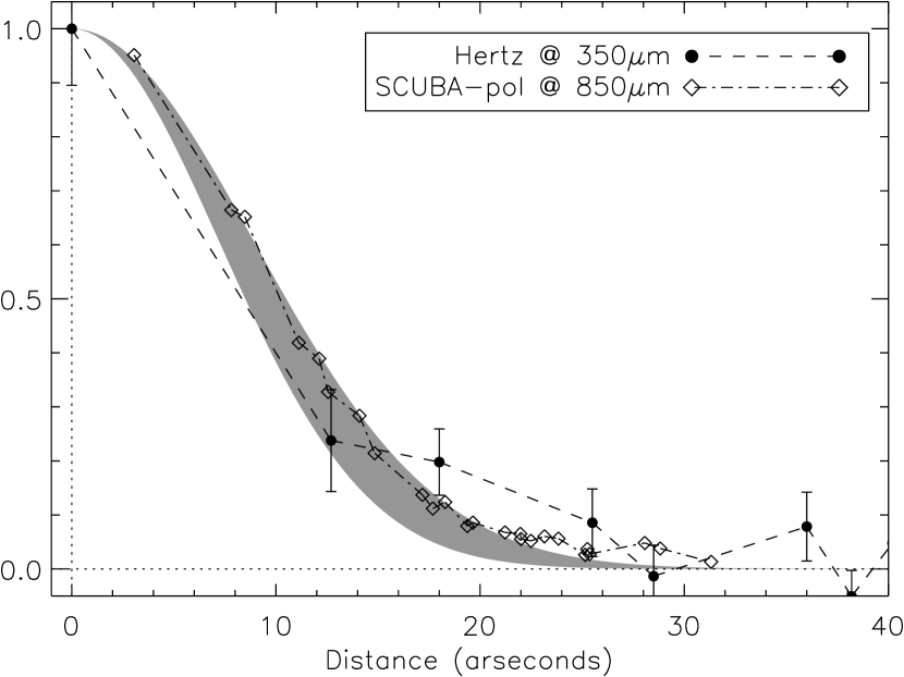
Figure 2: The Hertz $350\,\micron$ (circles and dashed line) and SCUBA-pol $850\,\micron$ (diamonds and dash-dotted line) beams were measured on Uranus in September 1997 and July 1998, respectively. In both cases the disk’s angular diameter was 3$\farcs$7. These data represent the effective beam-widths after all data processing steps. Gaussian beams with full-widths at half-maximum ranging from $17\arcsec$ – $21\arcsec$ are shown for comparison (gray). Error-bars on the Hertz data indicate the variation of the signal within an annulus centered at each radius (Dowell et al., 1998). Error-bars on the SCUBA-pol points were calculated from intensity uncertainties at each data pixel and are smaller than the plotted data points.

The SCUBA camera and polarimeter is described in detail elsewhere (Greaves et al., 2003; Jenness et al., 2000; Holland et al., 1999). Briefly, the $850\,\micron$ SCUBA-pol instrument consists of a single detector array with 37 pixels arranged on a hexagonal grid with a $2\farcm 3$ field-of-view; the polarization is measured by inserting a warm wire-grid, modulated by a stepped HWP. Fully-sampled polarimetric and photometric maps are generated by “jiggle-mapping” which moves the array by sub-pixel steps. The data analysis involves combining the individual jiggle maps and re-sampling them onto an output grid with a $6\arcsec$ pitch. Generation of fully-sampled maps in this manner also alleviates the need to follow sky-rotation throughout the night. While the intrinsic SCUBA beam size at $850\,\micron$ is close to the $14\arcsec$ diffraction limit of the JCMT, this map-making process results in an effective beam-size closer to $20\arcsec$ (Figure 2).

As noted above, the resultant spatial resolution for both Hertz at $350\,\micron$ and SCUBA-pol at $850\,\micron$ is $\approx 20\arcsec$. We refer to this resolution as the effective beam-width, which should not be confused with the diffraction limited resolution of the respective telescopes. Direct comparisons of the two beams measured on Uranus are shown in Figure 2. (The size of Uranus at the time of each measurement was $3\farcs 7$.) Gaussian-fits to these profiles yield $19\farcs 5\pm 0\farcs 1$ for SCUBA-pol and $19\arcsec\pm 2\arcsec$ for Hertz; the reported statistical uncertainties follow from a formal non-linear fit to the gaussian profile. These beamsizes are consistent with the measurements reported by Dowell et al. (1998) for Hertz ($20\arcsec\pm 2\arcsec$) and Di Francesco et al. (2008) for SCUBA (a primary beam of $19\farcs 5$). Given this beam similarity we have made no correction for different spatial resolutions when comparing these data sets.

The Hertz data are undersampled. However, since the SCUBA data are fully-sampled, there is sufficient information to estimate the SCUBA intensity and polarization at the same sky locations of the Hertz data. This is accomplished by reducing the SCUBA-pol data in the same manner as presented in Matthews et al. (2009) but choosing to output the data to grids and map-center locations which match the Hertz dataset. Table 1 lists the objects observed by both Hertz and SCUBA-pol at 350 and 850 $\micron$; Table 2 (in the electronic version only) gives a more complete list of the locations within each of the clouds. Table 2 also includes data for all points at both wavelengths for the polarization magnitudes and their ratio $P(850)/P(350)$, position angles and their difference $\phi(850)-\phi(350)$, intensity values and their ratio $F(850)/F(350)$, and uncertainties on all values. All polarization magnitudes in Table 2 have been corrected for positive bias (Section 2.2). The best estimates of those values is sometimes zero; as a result the ratio $P(850)/P(350)$ is reported as Nan for cases in which $P(850)$$=$$P(350)$$=$0, Inf for cases in which only $P(350)=0$, and equal to zero when only $P(850)=0$.

Table 1: Object Summary and Polarization Ratios

		data satisfying $P_{\mathrm{c}}>0$				data satisfying $P_{\mathrm{c}}\geq 3\sigma_{p}$				…also satisfying $|\Delta\phi|\tablenotemark{c}<10\arcdeg$
Source	Total	Number	Median	MAD		Number	Median	MAD		Number	Median	MAD
W3	0091	0058	2.2	1.1		014	2.5	0.8		04	2.0	0.3
NGC 1333	0154	0070	2.1	1.4		003	3.5	1.8		01	6.5	$\cdots$
OMC-1	0240	0203	1.6	0.7		136	1.6	0.6		65	1.6	0.5
OMC-2	0090	0054	1.9	0.9		010	2.4	0.6		02	2.6	0.3
OMC-3	0099	0082	2.3	1.1		035	2.0	0.8		15	1.6	0.6
NGC 2024	0104	0072	2.3	0.9		019	2.8	0.6		05	2.2	0.2
NGC 2068 LBS 10	0062	0045	1.7	0.6		023	1.9	0.5		07	1.9	0.8
NGC 2068 LBS 17	0062	0024	1.6	0.6		000	$\cdots$	$\cdots$		00	$\cdots$	$\cdots$
NGC 2071	0050	0018	4.0	2.0		001	2.4	$\cdots$		00	$\cdots$	$\cdots$
Mon R2	0076	0058	3.2	1.4		022	2.8	0.9		01	1.0	$\cdots$
Mon OB1 12	0066	0047	3.7	2.1		011	4.8	1.6		01	9.8	$\cdots$
$\rho$ Oph	0100	0076	1.7	0.8		025	1.3	0.4		07	1.3	0.5
IRAS 16293$-$2422	0063	0018	5.2	1.9		000	$\cdots$	$\cdots$		00	$\cdots$	$\cdots$
NGC 6334A	0059	0037	2.7	1.6		005	3.0	0.5		02	4.3	1.8
W49 A	0055	0046	2.6	1.4		023	2.4	0.9		07	2.7	0.8
W51 A (G49.5-0.4)	0112	0074	3.6	2.2		015	4.5	2.6		02	6.0	4.2
DR 21	0216	0142	1.6	0.6		056	1.6	0.4		22	1.6	0.4
DR 21 (Main)	0100	0072	1.7	0.6		036	1.6	0.5		14	1.6	0.4
All	1699	1124	2.1	1.0		398	1.9	0.7		141	1.7	0.6

Note. — The median polarization ratios ($P[850]/P[350]$), the median absolute deviation of their distribution (MAD; eq. [2]), and the number of data points in each sample are shown here. The column labeled “$P_{\mathrm{c}}>0$” indicates regions where the measured data satisfy $P_{\mathrm{m}}/\sigma_{p}>\sqrt{2}$ at both wavelengths (see Section 2.2). Columns labeled “$P_{\mathrm{c}}\geq 3\sigma_{p}$” indicate only data points satisfying that signal-to-noise criterion at both wavelengths; these values are calculated after applying the de-biasing technique discussed in Section 2.2. The columns labeled “also $|\Delta\phi|<10\arcdeg$” satisfy both the latter $P/\sigma_{p}$ constraint as well as the additional $\Delta\phi$ criterion. Source coordinates can be found in Table 1 of Dotson et al. (2010).

2.2 Positive Polarization Bias

By definition, the polarization amplitude is a positive-definite quantity. As a result, a noisy measurement of a truly zero-polarization source will result in a mean positive polarization. While there is no exact analytical method to correct for this bias many authors use the formula: $P_{\mathrm{c}}\approx(P^{2}_{\mathrm{m}}-\sigma_{p}^{2})^{1/2}$, where $P_{\mathrm{c}}$ is the bias-corrected polarization, $P_{\mathrm{m}}$ is the measured polarization, and $\sigma_{p}$ is the measured polarization uncertainty. Vaillancourt (2006; also Simmons & Stewart 1985; Quinn 2012) showed this was a good estimator when $P_{\mathrm{m}}\gtrsim 3\sigma_{p}$ but that $P_{\mathrm{c}}=0$ was a better estimator if $P_{\mathrm{m}}/\sigma_{p}\leq\sqrt{2}$. Matthews et al. (2009) applied the formula for high signal-to-noise to all their $850\,\micron$ data while Dotson et al. (2010) applied no corrections to their $350\,\micron$ data. For the data presented in this work we set $P_{\mathrm{c}}=0$ in cases where $P_{\mathrm{m}}/\sigma_{p}\leq\sqrt{2}$ and apply the above formula for data with $P_{\mathrm{m}}/\sigma_{p}>\sqrt{2}$. When computing signal-to-noise cuts on $P/\sigma_{p}$ in Table 1 and the following sections we use the corrected values $P_{c}$ as described above. The conclusions drawn in Sections 3 and 4 use only the $P_{\mathrm{c}}\gtrsim 3\sigma_{p}$ sample and are therefore not effected by the fact that the correction does not provide the best estimate within the regime $\sqrt{2}\leq P/\sigma_{p}<3$.

The corrections on $P$ have no effect on estimates of the polarization position angle; that is in the sense that there is no bias in the angle estimate as there is for the polarization amplitude. However, there is necessarily an effect on the angle uncertainty (e.g., Naghizadeh-Khouei & Clarke 1993). For example, in cases where the $P_{\mathrm{m}}/\sigma_{p}\leq\sqrt{2}$ the best estimate is $P_{\mathrm{c}}=0$ and thus any angle measurement is meaningless. We have made no attempt to estimate “corrected” angle uncertainties in Table 2. Such corrections are small for high signal-to-noise data (Naghizadeh-Khouei & Clarke, 1993) and therefore they will have little effect on our analysis and discussions below which use only data with $P_{\mathrm{c}}\gtrsim 3\sigma_{p}$.

3 Comparison

Maps comparing the $350\,\micron$ and $850\,\micron$ polarization data in each region are shown in the Appendix. Here we concentrate on quantitative comparisons of the polarization magnitudes and angles between the two different wavelengths.

The uncertainties on individual polarization measurements and on combined quantities like their angle differences and ratios can be quite large. In the measurements below we concern ourselves with the question of whether the observed distributions arise solely from measurement uncertainties or also have significant contributions from intrinsic variations across the clouds and/or locations within those clouds. To do this we define the reduced-$\chi^{2}$:

$$\chi^{2}_{r}=\frac{1}{N-1}\sum_{i=1}^{N}\frac{(x_{i}-x_{\mathrm{m}})^{2}}{\sigma_{i}^{2}}$$ (1)

where $x_{\mathrm{m}}$ is the median value of the samples $x_{i}$, $\sigma_{i}$ is the measurement uncertainty on the quantity $x_{i}$, and $N$ is the total number of data points in the sample.

3.1 Polarization Angles

One of the most obvious aspects of the polarizations presented in the maps is the agreement, or disagreement, of the position angles between the two wavelengths. Figure 3 compares these angles across the entire data-set and within three clouds with the largest number of data points. All the distributions peak near angle differences of zero degrees, that is $\Delta\phi\equiv\phi(850)-\phi(350)=0\arcdeg$. For all non-zero polarization data (i.e., data where both $P(350)>0$ and $P(850)>0$) the median angle difference is $1\arcdeg$ with a standard deviation of $39\arcdeg$. This agreement is stronger (i.e., has a smaller deviation) if we limit ourselves to only points with $P\geq 3\sigma_{p}$ (398 points in the entire data set). In this case the median angle difference is $4\arcdeg$ with a standard deviation of $28\arcdeg$.

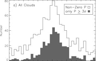
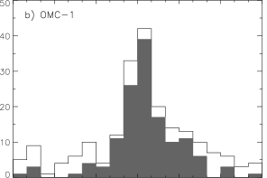
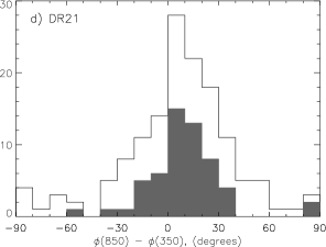
Figure 3: Histograms of the 850-to-350 $\micron$ polarization angle differences, $\phi_{850}-\phi_{350}$, for a) all clouds in this work, b) OMC-1, c) OMC-3, and d) DR 21. In each panel histograms are shown for all non-zero polarization data (open histograms) and only data satisfying $P\geq 3\sigma_{p}$ (gray histograms). The bin-widths for (a) are $5\arcdeg$, all others are $10\arcdeg$. The total number of data points in each sample is given in Table 1.

To rule-out the possibility that the width of the angle distribution is strongly dependent on the measurement uncertainties we calculate the $\chi_{r}^{2}$ value of the angle differences following equation (1). If most data points were consistent with the median angle difference within their uncertainties then we would expect $\chi_{r}^{2}\sim 1$ (especially for $N-1=397$ degrees-of-freedom for the entire $3\sigma$ data-set). However, for the complete data set with $P\geq 3\sigma_{p}$ we find $\chi_{r}^{2}=14$. From this we conclude the distribution’s width is intrinsic and not a result solely of data uncertainties.

Most of the clouds in our sample have insufficient data to perform this analysis separately on individual clouds. Exceptions to this point are OMC-1, OMC-3, and DR 21, whose angle distributions are also shown in Figure 3. For data satisfying the $P\geq 3\sigma_{p}$ criterion in those three clouds the median angle differences and standard deviations are $3\arcdeg\pm 25\arcdeg$, $4\arcdeg\pm 19\arcdeg$, and $10\arcdeg\pm 22\arcdeg$, with $\chi^{2}_{r}$ values of 18, 5, and 7, respectively. Therefore, as was observed for the entire data set above, the width of the angle-difference distribution ($\Delta\phi$) in these individual clouds is real, in the sense that they are not a result solely of the measurement uncertainties.

Lastly, we should note that the position angle rotations observed in these clouds are unlikely to be the result of Faraday rotation. In typical interstellar cloud conditions, at these wavelengths, Faraday rotation is generally much smaller than that observed here (e.g., Schleuning et al. 2000; Matthews, Wilson, & Fiege 2001).

3.2 Polarization Ratio

Table 1 lists the total number of locations where measurements were made at both wavelengths. For the best comparisons we typically choose to include only data satisfying the signal-to-noise criterion $P\geq 3\sigma_{p}$; this criterion is applied after the de-biasing correction discussed in Section 2.2. Figure 4a shows the distribution of these points. This figure shows all data satisfying the $3\sigma_{p}$ criterion, including outliers as high as $P(850)/P(350)=31$; the inset concentrates on the main peak.

As can be seen in Figure 4 the distributions are non-normal in nature and often contain outliers away from the main peaks. Therefore, unlike the polarization angle distributions in Section 3.1, none of these distributions are well characterized by a simple sample mean or a sample standard deviation. As robust descriptions of the distributions’ central tendencies and width we use the samples’ medians and median absolute deviations (MAD). The MAD of a set of measurements $x$ is defined as the median value of the residuals, where the residuals are also calculated with respect to the sample median; that is

$$\mathrm{MAD}\equiv\mathrm{median}\left(|x-x_{\mathrm{m}}|\right).$$ (2)

where $x_{\mathrm{m}}$ is the median value of the measurements $x$. For a normal distribution the MAD is significantly smaller than its standard deviation ($\sigma$) with an expectation value of $\sigma/1.48$. However, given the small-number of comparison points in many of the clouds in Table 1 and that the $P(850)/P(350)$-distribution is not expected to be symmetric we report only the MADs there.

The complete $3\sigma$ data set contains 398 points with a median $P(850)/P(350)$ value of 1.9, MAD=0.7, and $\chi^{2}_{r}$$=$$9$. The $\chi_{r}^{2}$-value implies that the distribution’s width is intrinsic and not a result solely of data uncertainties. We reach the same conclusion examining the distributions for OMC-1, OMC-3, and DR21. (Medians are shown in Table 1, $\chi_{r}^{2}=$ 12, 5, and 3.)

We note that many of the peaks in the distributions of Figure 4 are clearly different from the medians listed in Table 1, this is mostly driven by some large outliers in the distribution. An alternate estimate of this peak is the value which minimizes the MAD. For the entire $3\sigma$ data-set in Figure 4a this alternative peak estimate is 1.5 with MAD=0.6. If the median in equation (1) is replaced with this peak then $\chi^{2}_{r}=6$. These peaks, new MAD’s, and $\chi^{2}_{r}$ of OMC-1, OMC-3, and DR21 are given in Table 3. Using these peaks yields $\chi^{2}_{r}>1$ for all three clouds and, therefore, does not change the conclusion that the distributions’ widths are intrinsic and not a result solely of data uncertainties. Also, the difference between the median and the peak is less than the MADs in all cases (i.e., the whole data-set and the three specific clouds); none of the discussion in Section 4 relies strongly on these precise values.

Table 3: Polarization Ratio Distributions

	data satisfying $P\geq 3\sigma_{p}$				…also satisfying $|\Delta\phi|<10\arcdeg$
Source	Peak	MAD	$\chi^{2}_{r}$		Peak	MAD	$\chi^{2}_{r}$
OMC-1	1.3	0.5	13.4		1.4	0.5	20.8
OMC-3	1.4	0.5	02.9		1.2	0.3	03.7
DR 21	1.4	0.4	02.5		1.8	0.3	05.2
DR 21(Main)	1.3	0.3	02.3		1.8	0.3	06.6
All	1.5	0.6	06.0		1.4	0.5	10.9

Note. — The peak value and the median absolute deviation (MAD) of the polarization ratio ($P[850]/P[350]$) distributions which minimize the MAD (eq. [2]). Also shown are $\chi^{2}_{r}$ values as calculated from equation (1); see Section 3.2. The columns labeled “$P\geq 3\sigma_{p}$” and “also $|\Delta\phi|<10\arcdeg$” are defined as in Table 1.

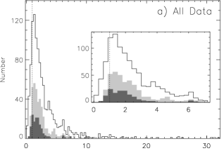
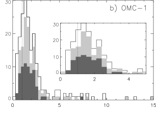
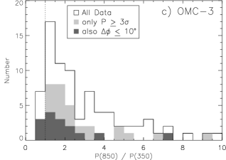
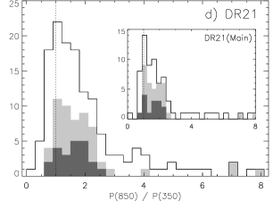
Figure 4: Histograms of the 850-to-350 $\micron$ polarization ratio for (a) all data in this work, (b) OMC-1, (c) OMC-3, and (d) DR 21. Each plot contains different cuts on the data as shown in the legend of (c): all data (open histogram), only $P\geq 3\sigma_{p}$ (light gray), $P\geq 3\sigma_{p}$ and $|\Delta\phi|\leq 10\arcdeg$ (dark gray). For reference vertical dotted lines are drawn at $P(850)/P(350)=1$. For display purposes only, the insets in (a) and (b) magnify the lower-end of the distributions where the histograms peak. Note the larger plot in (d) contains all data in DR21 while the inset shows only data in DR21(Main). The bin-widths for (c) are 0.5, all others are 0.3. The total number of data points in each sample is given in Table 1.

In using the polarization ratio to study grain alignment (e.g., Section 4.2) we want to ensure that data at both wavelengths are sampling the same regions of the cloud, both along the line-of-sight (LOS) and across the plane-of-the-sky (POS). The latter criterion is simply met due to the fortuitous ability to beam-match the 350 and 850 $\micron$ data. If the emission sources are the same for radiation at both 350 and 850 $\micron$ then the former criterion would also be met. Meeting this criterion is more difficult, but we try to limit its effect by choosing data with little-to-no position angle rotation between the two wavelengths. For this reason our analysis is often limited to data points where $|\Delta\phi|\leq 10\arcdeg$. Note that $\sigma_{\phi}\leq 10\arcdeg$ corresponds to data points with $P\gtrsim 3\sigma_{p}$.

To understand this particular data-cut, consider the case where the magnetic field changes its orientation along the line-of-sight (and within the cloud depths sampled by at least one wavelength). This may result in a wavelength-dependent change in both the polarization position angle (which follows the change of the field’s projected orientation) and the polarization level (due to the field’s changing inclination angle). In interpreting the polarization spectrum in terms of grain alignment physics, we wish to eliminate the changing inclination angle as the cause of any change in the polarization level (which can also result from other grain/cloud properties; see Section 4.2). Since a changing field orientation must occur for any data with a wavelength-dependent angle, we can eliminate regions where this occurs by removing such data. While this does not ensure that points without wavelength-dependent angles arise from a single source it is unlikely, in the statistical sense, that the LOS field angles can change for many points in our large sample without an accompanying POS rotation.

Table 1 shows the total number of data points satisfying both the $P/\sigma_{p}\geq 3$ and $|\Delta\phi|\leq 10\arcdeg$ data-cuts in each cloud, along with their median polarization ratios and median absolute deviations. After making this second data cut the number of surviving data points drops to 141, only 35% of the $3\sigma$ dataset. The resulting median ratio is $P(850)/P(350)=1.7$ with MAD=0.6 and $\chi_{r}^{2}=11$ (see Figure 4a). The $\chi_{r}^{2}$ values for OMC-1, OMC-3, and DR21 are also large using this data cut ($\chi_{r}^{2}=$ 19, 5, and 3, respectively), again implying that the distributions’ widths are not a result solely of data uncertainties. There are not as many outliers in the distributions after the $|\Delta\phi|$-cut as their were in the $3\sigma$-only cut. These do have some effect on the measured MADs (as discussed earlier in this section); Table 3 reports the distribution peaks, MADs, and revised values of $\chi_{r}^{2}$ for the $|\Delta\phi|$-cut in the case where we have minimized the MADs. These small changes in the distribution widths still result in values of $\chi_{r}^{2}\gtrsim 1$ meaning that our conclusion, that the widths are intrinsic and not a result solely of data uncertainties, still holds.

4 Discussion

4.1 The Polarization Spectrum

Figure 5 shows an updated version of the polarization spectrum from Vaillancourt (2002) and Vaillancourt et al. (2008). All the data in this figure satisfy the criteria $P\geq 3\sigma_{p}$ and $|\Delta\phi|\leq 10\arcdeg$. Here we plot the median value of DR21(Main), rather than DR21, as the data at other wavelengths ($1300\,\micron$) only cover that region of the cloud. While all the data in Figure 5 show $P(850)>P(350)$ we would draw the reader’s attention to the range of ratios plotted in the distributions of Figure 4. For example, the median ratio for all clouds in this work is plotted at $P(850)/P(350)=1.7$ but has a relatively large MAD (0.6).

The previous work comparing Hertz and SCUBA-pol performed by Vaillancourt (2002) and Vaillancourt et al. (2008) were based on slightly different data sets than we use here. First, the earlier results were obtained using the data prior to the systematic re-analyses performed by Dotson et al. (2010; see also Kirby et al. 2005) and Matthews et al. (2009). Second, those results attempted to match the Hertz and SCUBA beams by smoothing the SCUBA data to match Hertz’s presumably larger beam size and re-sampled at a rate of 5 arcseconds per pixel. Given the pointing accuracies of Hertz (4″–6″; Dowell et al. 1998) and SCUBA (2″) the $5\arcsec$ re-sampling was not unreasonable. However, as shown in Figure 2, the smoothing step was likely unnecessary. Despite these analysis differences the median results are in good agreement. For data satisfying $P\geq 3\sigma_{p}$ and $|\Delta\phi|\leq 10\arcdeg$ the previous work found $P(850)/P(350)$ medians and standard deviations of $1.4\pm 0.6$ and $1.7\pm 2.7$ for OMC-3 and DR 21(Main), respectively (Vaillancourt, 2002). Here we find medians and MADs of $1.6\pm 0.6$ and $1.6\pm 0.4$ for those two clouds. The large difference in the DR21(Main) standard deviations (=1.5 for the current work) likely lies in the fact that the earlier $850/350$ data comparison used a different set of DR21 data. The analysis by Matthews et al. (2009) used additional observations not available at the time of Vaillancourt (2002) and the analysis resulted in better rejection of noisy data.

For W51, Vaillancourt et al. (2008) found $1.8\pm 2.4$ (median and standard deviation). This is consistent with the W51 results shown in Table 1, $6.0\pm 4.2$ (median and MAD), but only because of the large deviations. These data are not plotted in Figure 5 as only two data points survive the data cuts.

The $P(850)/P(350)$ ratio for OMC-1 is calculated in this work for the first time. Figure 5 also includes $P(450)/P(350)$ (solid triangle; Vaillancourt et al. 2008) and $P(100)/P(350)$ (open triangle; Vaillancourt 2002) data points. The OMC-1 cloud is thus the only cloud in our data set which includes data both above and below the $350\,\micron$ minimum in the spectrum.

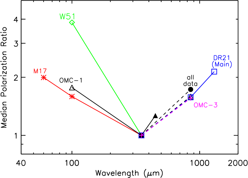
Figure 5: Polarization spectrum in several molecular clouds, normalized at $350\,\micron$. The $P(850)/P(350)$ data in this work are shown as dotted lines; note that OMC-1, OMC-3, and DR21(Main) have identical medians (see Table 1). The solid circle represents the median of all data in this work. All data in this plot, including that shown here for the first time, meet the $3\sigma_{p}$ and $\Delta\phi$ criteria described in the text. Data at $\lambda<350\,\micron$ and that for DR21(Main) at $P(1300)/P(350)$ are from Vaillancourt (2002). All data used at $350\,\micron$ are from Hertz (Dotson et al., 2010) with the exception of the OMC-1 point comparing 350 and 450 $\micron$ (solid triangle) which is from SHARP (Vaillancourt et al., 2008). For clarity no error bars are shown here, but see Figure 4 for the distributions. [A color version of this figure is available in the electronic version.]

4.2 Grain Alignment

The original work by Hildebrand et al. (1999) made it clear that the simplest model, isothermal dust populations all with the same polarization and/or alignment properties, can not reproduce a spectrum like that in Figure 5. In fact such a model yields a polarization spectrum independent of wavelength beyond 50 µm. In order to explain such a spectrum we consider that a number of physical mechanisms are responsible for the absolute polarization level observed in dust emission. Foremost among these are the efficiency with which dust grains become aligned with magnetic fields and variations in the inclination of that field to the line-of-sight. Ideally, our $|\Delta\phi|\leq 10\arcdeg$ data cut (Section 3.2) has eliminated the field inclination as a variable in the observed spectrum, leaving alignment efficiency as the key variable.

In order to generate wavelength-dependent polarization spectra the alignment efficiencies must be correlated (or anti-correlated) with changes in the grains’ emission. In order to explain spectra like those in Figure 5 Hildebrand et al. (1999) considered simple emission laws of the form $F(\nu)\propto\nu^{\beta}B_{\nu}(T)$, where $\nu$ is the observed frequency, $\beta$ the spectral index, and $B_{\nu}(T)$ is the Planck function at temperature $T$. For such models the required change in emission can take the form of differences in temperature, differences in the spectral index, or a combination of the two (see also Vaillancourt 2002, 2007). Below we discuss two physical models of the ISM and molecular clouds, both of which result in grain populations with the different alignment properties and temperatures/spectral-indices which lead to wavelength-dependent polarization spectra.

Theoretical models of grain alignment have a long history (see reviews by Lazarian 2003, 2007; Hildebrand 1988) with detailed observational tests possible only very recently (e.g., Lazarian, Goodman, & Myers 1997; Matsumura & Bastien 2009; Andersson & Potter 2010; Andersson et al. 2011; Matsumura et al. 2011). In one of the most recent models, that of “radiative alignment torques” (RAT; Cho & Lazarian 2005; Lazarian & Hoang 2007; Hoang & Lazarian 2008, 2009a, 2009b) stellar and interstellar photons provide the necessary torques to align the spin-axes of dust grains parallel to the local magnetic field. Bethell et al. (2007) simulated a molecular cloud containing aspherical graphite and silicate grains with a typical interstellar grain-size distribution (i.e., Mathis, Rumpl, & Nordsieck 1977) and radii of 0.005–0.5 µm. The RAT model results in alignment only of grain sizes larger than some cut-off, the exact value of which is dependent on properties like the gas density and radiation field and can vary throughout the simulated cloud (Cho & Lazarian, 2005). As the larger grains are more efficient emitters they reach cooler temperatures than the smaller grains in equilibrium. This yields an anti-correlation between grain temperature and alignment; the small warm grains are unaligned while the large cool grains are aligned. The resulting polarization spectrum rises from 100 to 400 $\micron$, with little variation at longer wavelengths. For the wavelengths of interest here they find $P(850)/P(350)\sim 1.0$–1.1.

Draine & Fraisse (2009) also present models composed of aspherical silicate grains and spherical graphite grains (here we discuss only their Model numbers 1 and 3). The grain-size distribution and the relative silicate-graphite mix are constrained by the observed interstellar extinction. Additionally, rather than model any physical alignment mechanism (such as RAT), their grain alignment is empirically constrained by the typical interstellar polarization spectrum spanning near-optical wavelengths (i.e., the “Serkowski law”). The result is similar to the work of Bethell et al. (2007) in the sense that larger grains are both cooler and better aligned than the smaller grains and produces a steep polarization spectrum in the 40 – 400 $\micron$ range. However, the Draine & Fraisse (2009) spectrum continues to rise beyond $400\,\micron$ such that $P(850)/P(350)\sim 1.2$–1.3. This long-wavelength behavior is a combination of a) the cooler silicate grains being aligned, whereas the warmer spherical graphite grains are not, and b) the shallower spectral indices of silicates compared to graphites.

The median $P(850)/P(350)$ values presented in this work (Fig. 5 and Table 1) are clearly steeper than the model estimates just discussed ($\sim 1.7$ for the “all clouds, $P$$>$$3\sigma$, $|\Delta\phi|$$<$$10\arcdeg$” sample). However, the data distributions are large and, therefore, cannot strongly rule-out either model. Additionally, the models are calculated using physical conditions and constraints which likely do not prevail in the real clouds studied here. The Draine & Fraisse (2009) model is constrained by data from the very low density ISM ($A_{V}\lesssim$ a few) whereas our sample of clouds is flux-limited to some very bright, dense Galactic regions ($A_{V}>20$). While modeling a “molecular cloud”, the Bethell et al. (2007) model bathes the cloud rather uniformly in a typical interstellar radiation field which may be quite different from real clouds containing embedded stars.

4.3 Embedded Sources

The RAT mechanism predicts that grains exposed to stronger radiation sources will be more efficiently aligned. From this we might expect to see systematic trends in the polarization with distance from stellar sources embedded in molecular clouds. Such a trend is hinted at in $60\,\micron$ polarization observations towards the W3A H II region (Schleuning et al., 2000). The most prominent embedded sources in OMC-1 are a group of sources coincident with the BNKL intensity peak and the Trapezium stars in the visible Orion nebula (Fig. 6). Using the MSX point-source catalog (Price et al., 2001; Egan et al., 2003) we have also identified a number of embedded sources in the DR21 cloud (Fig. 7). However, the proximity of the sources to each other, coupled with the fairly low spatial resolution of the polarization maps, does not allow a careful quantitative study of the strength of the polarization (at either wavelength) or the polarization ratio as a function of distance from these sources.

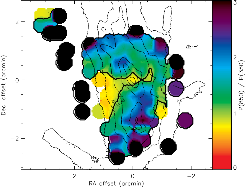
Figure 6: Map of the polarization ratio, $P(850)/P(350)$, in OMC-1. This map includes only $P\geq 3\sigma_{p}$ data but includes points typically rejected by the $|\Delta\phi|$ criterion discussed in the text. Data with $P(850)/P(350)>3$ are shown as saturated (black) pixels. Thin contours denote the $350\,\micron$ intensity at levels of 1, 4, 8, 20, 40, and 80 % of the peak intensity (data from SHARC-2; Vaillancourt et al. 2008). The thick contour is drawn at $P(850)/P(350)=1$. For reference we also show the four Trapezium stars of M42. [A color version of this figure is available in the electronic version.]

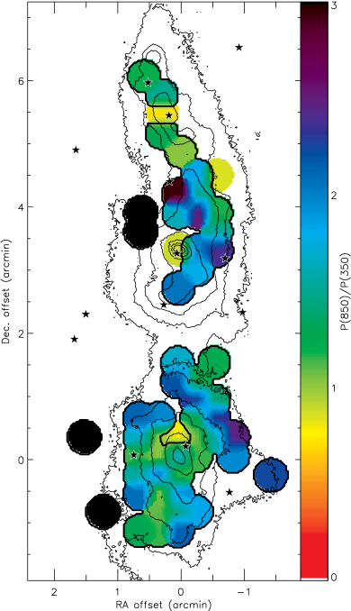
Figure 7: Same as Figure 6 but for DR21. Intensity data are from SHARC-2 (D. Dowell, private communication) Black stars indicate point sources identified by MSX (Section 4.3). [A color version of this figure is available in the electronic version.]

A trend in polarization efficiency with distance from a radiation source also implies a correlation between the observed polarization and dust temperature. A careful measure of the dust temperature requires SED measurements over a wide range of wavelengths, a task which is beyond the scope of the present work (e.g., Vaillancourt 2002). To some extent, one can consider the intensity or flux density ratio, $F(850)/F(350)$, as a proxy for the temperature. Figures 8a and 8b compare the intensity ratio in OMC-1 and DR21 to the polarization at both 350 and 850 $\micron$. The polarization in both clouds generally drops with increasing intensity ratio. If we interpret these ratios as color temperatures then the polarization increases with increasing temperature, as would be expected for grains aligned via RAT. However, we caution against over-interpretation of this result as defining a color-temperature is problematic in the dense clouds for at least two reasons. First, the range plotted in Figure 8 corresponds to unrealistically large temperatures; assuming $\beta=2$ then $T=13$ K for the largest ratio $F(850)/F(350)=0.1$ is reasonable but $T>100$ K for ratios $F(850)/F(350)<0.033$. Secondly, the ratio may also be the result of changes in grain emissivity (i.e., spectral index) and column density as well as the temperature.

Figure 8: Polarization vs. intensity ratio in OMC-1 (a), DR21 (b), and all data except OMC-1 and DR21 (c). Here we plot only data meeting the $P/\sigma_{p}$ and $|\Delta\phi|$ criteria described in the text. The lines are power-law fits to the data (solid line for $350\,\micron$, dashed line for $850\,\micron$); fits do not consider error bars. In (a) the fits exclude those points within $20\arcsec$ of OMC-1’s central intensity peak (solid circles and solid triangles; see Section 4.4).

Using the intensity ratio as a proxy for temperature also has the advantage that it is independent of distance, allowing us to combine the relatively sparse data in individual clouds into a larger dataset. Combining the remaining data in clouds other than DR21 or OMC-1 results in Figure 8c. The same trend of falling polarization is seen at both wavelengths. We emphasize that we are comparing the polarization with the intensity ratio and are not discussing the “polarization-hole” effect which is often observed when comparing the polarization to absolute intensity at any given wavelength (e.g., Schleuning 1998; Matthews, Fiege, & Moriarty-Schieven 2002).

4.4 Intensity and Polarization Ratios

One difficulty in using the absolute polarization values in Section 4.3 above is that the observed polarization magnitude is also a function of the parameters like the magnetic field’s LOS inclination angle, grain cross-section, and turbulence, all of which may vary spatially across the cloud. The inclination angle effect is mitigated somewhat by our choice to limit the data set to those points with $|\Delta\phi|\leq 10\arcdeg$ (see Section 3.2). These effects can be further mitigated by using the ratio $P(850)/P(350)$. If the same grains are responsible for the polarized emission at both wavelengths then those “polarization reduction” factors effectively cancel in the polarization ratio (Hildebrand et al., 1999).

Figures 6 and 7 show the spatial distributions of the polarization ratio in OMC-1 and DR21, respectively. Most of the mapped areas are characterized by polarizations which are larger at $850\,\micron$ than $350\,\micron$. Notable exceptions are intensity peaks in both objects (BNKL at the origin of the OMC-1 map and DR21-OH(Main) at [$+3\farcs 3,0$] in the DR21 map). The OMC-1 peak has also shown differences from the rest of the cloud in other polarization work (e.g., Rao et al. 1998; Vaillancourt 2002; Vaillancourt et al. 2008) so we will omit data within $20\arcsec$ (one beam) of the peak in the analysis below.

The most direct tests of the grain alignment models using submillimeter data require comparisons between the measured polarization ratio and the dust temperatures, spectral indices, and/or radiation environment of the aligned grains. A careful measure of those parameters requires SEDs measured over a wide range of wavelengths, a task which is beyond the scope of the present work (e.g., Vaillancourt 2002). However, we can again use the intensity ratio, $F(850)/F(350)$, as a proxy for the temperature or spectral index. Very different trends are observed when comparing this ratio to the polarization ratio in OMC-1 and DR21 (Figures 9a and 9b). The trend is an increase in $P(850)/P(350)$ in OMC-1 but a decrease in DR21. As before the intensity ratio is independent of distance, allowing us to combine the remaining data in clouds other than DR21 or OMC-1 (Fig. 9c). No strong trend between the intensity ratio and polarization ratio is observed.

The large amount of scatter in these observations is not unexpected. The dense clouds studied here are certainly composed of multiple temperature components covering a wide range (e.g., $\sim 20$ – 80 K). Therefore, the intensity ratio is a measure not only of the components’ dust temperatures, but also their different spectral indices and relative column densities. Presumably this effect is partly the cause of the large scatter observed in the data of Figure 9.

Figure 9: Polarization and intensity ratios in OMC-1 (a), DR21 (b), and all data except OMC-1 and DR21 (c). The upper $x$-axis scales cast the intensity-ratio as the standard spectral index defined through the relation $F(\nu)\propto\nu^{\beta+2}$. Here we plot only data meeting the $P/\sigma_{p}$ and $|\Delta\phi|$ criteria described in the text. The lines are power-law fits to the data; in (a) the fits exclude those points within $20\arcsec$ of OMC-1’s central intensity peak (solid circles; see Section 4.4).

5 Summary

We have compiled all the spatially coincident data available from the Hertz ($350\,\micron$; Dotson et al. 2010) and SCUBA ($850\,\micron$; Matthews et al. 2009) polarimeters. In order to facilitate this comparison the SCUBA-pol data have been spatially re-sampled to match the spatial locations of the Hertz data; the two instruments have comparable spatial resolution ($20\arcsec$). We find a total of 1699 individual locations which can be compared within 17 different Galactic clouds; all the polarization and intensity data at 350 and $850~{}\micron$ are given in electronic format in Table 2. Of these data 1124 points yield non-zero polarizations at both wavelengths when corrected for the positive polarization bias. Additionally, of the bias-corrected data, 398 points satisfy the criterion $P/\sigma_{p}\geq 3$ at both wavelengths, and 141 points satisfy the additional criterion $|\phi(850)-\phi(350)|\leq 10\arcdeg$. Complete polarization and intensity maps for all clouds are given in the Appendix.

We have investigated the change in polarization angle from 850-to-$350~{}\micron$. The angle differences exhibit a wide distribution indicating that, in some regions, there is a real angle rotation within the measurement uncertainties. However, the angle distributions are centered about $\phi(350)\approx\phi(850)$. These conclusions hold globally for the entire $P/\sigma_{p}\geq 3$ data set in this work and individually for the $P/\sigma_{p}\geq 3$ data sets in the clouds OMC-1, OMC-3, and DR21. Due to the limited number of data points in other individual clouds we have made no attempt to study the angle distributions nor the point-by-point angle agreement between wavelengths; therefore these conclusions do not necessarily extend to the other clouds included herein.

We have also examined the 850-to-$350~{}\micron$ polarization ratio, $P(850)/P(350)$, on a point-by-point basis at every spatial location in each of our sampled clouds. From this work we establish a genuine trend towards higher polarization at $850\,\micron$ than $350\,\micron$ with a median polarization ratio of $P(850)/P(350)=1.7$ (and a median absolute deviation of 0.6). These values cover all clouds in our dataset and points which satisfy the criteria $P/\sigma_{p}\geq 3$ and also $|\phi(850)-\phi(350)|\leq 10\arcdeg$. This trend is consistent with previous work (e.g., Hildebrand et al. 1999; Vaillancourt 2002; Vaillancourt et al. 2008) and is best explained by models which require mixtures of dust grains with different physical properties (i.e., temperatures and spectral indices) and different alignment efficiencies. The dust and alignment models of Bethell et al. (2007) and Draine & Fraisse (2009) predict increasing values for the polarization from 350-to-$850~{}\micron$ ($\sim 1.0$–1.3) but not of the same magnitude as observed here. This is most likely due to the fact that their models use very different physical conditions than prevail in our sample of bright, dense molecular clouds.

We find a trend in which the 350 and 850 $\micron$ polarizations tend to fall as the 850-to-350 $\micron$ intensity ratio increases. If we interpret this ratio as a color temperature then these data are consistent with a key prediction of radiative alignment torques. That is, grains which are more exposed to radiation sources, and are thus warmer, are more efficiently aligned. However, we caution that the assignment of temperature to a two-wavelength intensity ratio is not robust. No clear trends are observed when the polarization ratios are compared to the intensity ratios on a point-by-point basis. Better tests require work at additional wavelengths in order to produce SEDS from which more accurate dust temperatures can be extracted.

Appendix A Polarization Maps

Figures 10–26 present grayscale/contour maps of intensity along with polarization vectors at $350\,\micron$ (blue lines) and $850\,\micron$ (red lines). Only vectors with $P\geq 3\sigma_{p}$ and $\sigma_{p}\leq 4\%$ are drawn on the maps; the latter criterion is an aesthetic choice to remove points with atypically large polarizations. Vectors spaced more closely than the nominal $17\farcs 8$ Hertz pixel pitch are a result of moving the Hertz array in sub-pixel steps. Additionally, some SCUBA-pol vectors in regions without Hertz coverage have not been plotted. Each map includes a scale-bar for determining the absolute polarization levels; the scale-bars differ for each map but are the same length for each wavelength within a map. Map center coordinates are given in Table 1 of Dotson et al. (2010).

As indicated in the figure captions most intensity maps are from SCUBA at $850\,\micron$ (Di Francesco et al., 2008). For aesthetic reasons some maps use $350\,\micron$ intensity data from Hertz, while OMC-1 and DR21 use $350\,\micron$ intensity data from the SHARC-2 camera at the CSO (Dowell et al., 2003). The lower-right corner of each map includes a gray-circle indicating the $20\arcsec$ effective beam-size of Hertz and SCUBA-pol. Note that this beam is for the polarization data only, not the intensity maps; SCUBA intensity maps typically have $19\arcsec$ resolution, Hertz intensity maps typically have $28\arcsec$ resolution, and SHARC-2 intensity maps typically have $10\arcsec$ resolution.

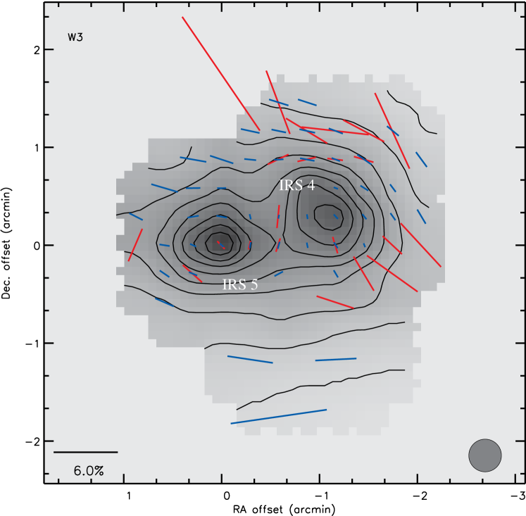
Figure 10: W3. The intensity map is from Hertz at $350\,\micron$ with contours drawn at 10, 20, 30, …, 90% of the peak intensity. Other key map features for this and subsequent figures are described in the text.

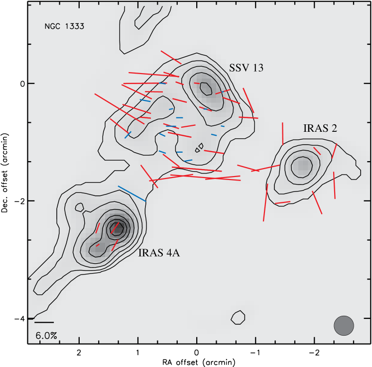
Figure 11: NGC 1333. The intensity map is from SCUBA with contours drawn at 2, 5, 10, 20, 40, 60, and 80% of the peak $850\,\micron$ intensity (which occurs in IRAS 4A).

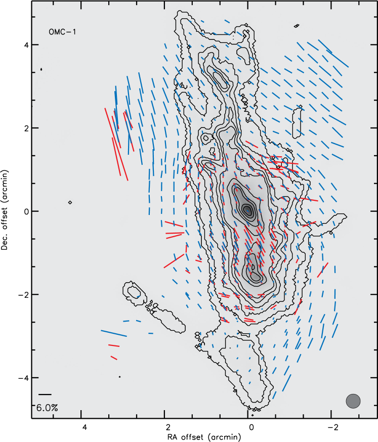
Figure 12: OMC-1. The intensity map is from SHARC-2 (Vaillancourt et al., 2008) with contours drawn at 1, 2, 4, 6, 8, 10, 20, 40, 60, and 80 % of the peak $350\,\micron$ intensity. The gray circle in the lower-right indicates the $20\arcsec$ effective beam-size of Hertz and SCUBA-pol, not the SHARC-2 intensity data which has a beam size of $\sim$10″.

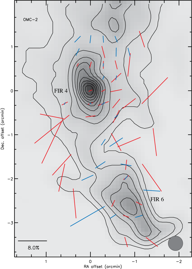
Figure 13: OMC-2. The intensity map is from SCUBA with contours drawn at 5, 10, 20, 30, …, 90% of the peak $850\,\micron$ intensity.

Figure 14: OMC-3. The SCUBA intensity is shown with contours at 10, 20, 30, 40, 60, and 80% of the peak $850\,\micron$ intensity. (Note that some SCUBA-pol vectors in the center of the map have been removed where there was no Hertz-coverage of this cloud.)

Figure 15: NGC 2024. The intensity map is from SCUBA with contours drawn at 5, 10, 20, 30, …, 90% of the peak $850\,\micron$ intensity.

Figure 16: NGC 2068 LBS 10. The intensity map is from SCUBA with contours drawn at 10, 20, 30, …, 90% of the peak $850\,\micron$ intensity. Cloud core labels are from Mitchell et al. (2001).

Figure 17: NGC 2068 LBS 17. The intensity map is from SCUBA with contours drawn at 10, 20, 30, …, 90% of the peak $850\,\micron$ intensity. Cloud core labels are from Mitchell et al. (2001).

Figure 18: NGC 2071. The intensity map is from Hertz with contours drawn at 20, 30, …, 90% of the peak $350\,\micron$ intensity.

Figure 19: Mon R2. The intensity map is from SCUBA with contours drawn at 10, 20, 30, …, 90% of the peak $850\,\micron$ intensity.

Figure 20: Mon OB1 IRAS 12 (IRAS 06382+0939). The intensity map is from SCUBA with contours drawn at 10, 20, 30, …, 90% of the peak $850\,\micron$ intensity. Cloud core labels are from Wolf-Chase et al. (2003)

Figure 21: $\rho$ Oph A. The intensity map is from SCUBA with contours drawn at 10, 20, 30, …, 90% of the peak $850\,\micron$ intensity.

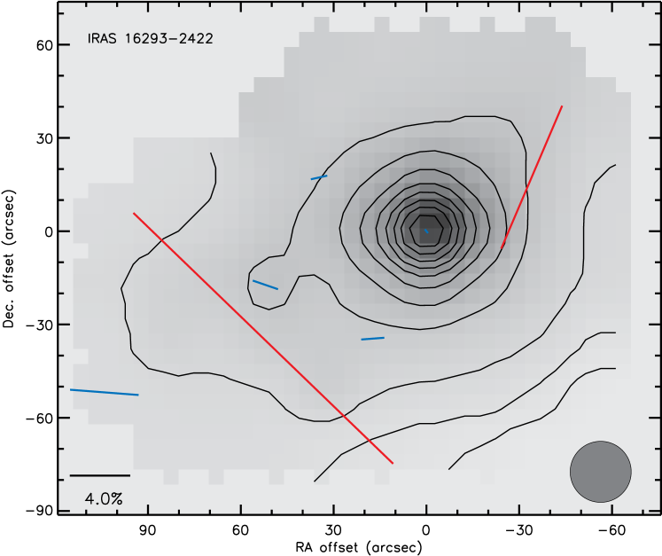
Figure 22: IRAS 16293$-$2422. The intensity map is from Hertz with contours drawn at 10, 20, 30, …, 90% of the peak $350\,\micron$ intensity.

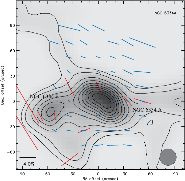
Figure 23: NGC 6334A. The intensity map is from SCUBA with contours drawn at 5, 10, 20, 30, …, 90% of the peak $850\,\micron$ intensity.

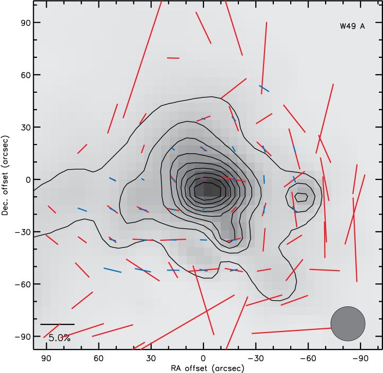
Figure 24: W49 A. The SCUBA intensity is shown with contours at 10, 20, 30, …, 90% of the peak $850\,\micron$ intensity.

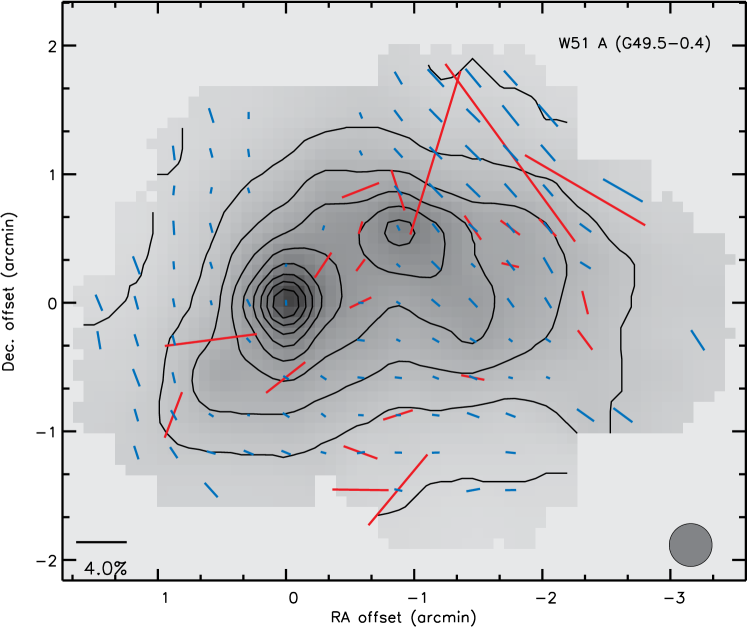
Figure 25: W51 A (G49.5-0.4). The Hertz intensity is shown with contours at 10, 20, 30, …, 90% of the peak $350\,\micron$ intensity.

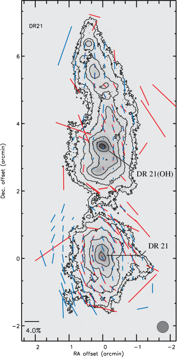
Figure 26: DR 21. The $350\,\micron$ intensity is shown in grayscale with contours drawn at 1, 2, 5, 10, 20, 40, and 80 % of the peak. Intensity data are from the SHARC-2 camera with a spatial resolution of $\approx 10\arcsec$ (C. D. Dowell, private communication). The gray circle in the lower-right indicates the $20\arcsec$ effective beam-size of Hertz and SCUBA-pol, not the SHARC-2 intensity data. The intensity peak is DR 21 OH (Main) and the southern peak at the map origin is DR 21 (Main).

References

- Andersson et al. (2011) Andersson, B.-G., Pintado, O., Potter, S. B., Straižys, V., & Charcos-Llorens, M. 2011, A&A, 534, A19
- Andersson & Potter (2007) Andersson, B.-G. & Potter, S. B. 2007, ApJ, 665, 369
- Andersson & Potter (2010) —. 2010, ApJ, 720, 1045
- Bethell et al. (2007) Bethell, T. J., Chepurnov, A., Lazarian, A., & Kim, J. 2007, ApJ, 663, 1055
- Cho & Lazarian (2005) Cho, J. & Lazarian, A. 2005, ApJ, 631, 361
- Crutcher (2004) Crutcher, R. M. 2004, in The Magnetized Interstellar Medium, eds. B. Uyaniker, W. Reich, & R. Wielebinski, 123
- Curran & Chrysostomou (2007) Curran, R. L. & Chrysostomou, A. 2007, MNRAS, 382, 699
- Davis & Greenstein (1951) Davis, L. J. & Greenstein, J. L. 1951, ApJ, 114, 206
- Di Francesco et al. (2008) Di Francesco, J., Johnstone, D., Kirk, H., MacKenzie, T., & Ledwosinska, E. 2008, ApJS, 175, 277
- Dotson et al. (2000) Dotson, J. L., Davidson, J., Dowell, C. D., Schleuning, D. A., & Hildebrand, R. H. 2000, ApJS, 128, 335
- Dotson et al. (2010) Dotson, J. L., Vaillancourt, J. E., Kirby, L., et al. 2010, ApJS, 186, 406
- Dowell et al. (2003) Dowell, C. D., Allen, C. A., Babu, R. S., et al. 2003, in Proc. SPIE 4855, Millimeter and Submillimeter Detectors for Astronomy, eds. T. G. Phillips & J. Zmuidzinas, 73
- Dowell et al. (1998) Dowell, C. D., Hildebrand, R. H., Schleuning, D. A., et al. 1998, ApJ, 504, 588
- Draine & Fraisse (2009) Draine, B. T. & Fraisse, A. A. 2009, ApJ, 696, 1
- Egan et al. (2003) Egan, M. P., Price, S. D., Kraemer, K. E., et al. 2003, The Midcourse Space Experiment Point Source Catalog Version 2.3 Explanatory Guide (AFRL-VS-TR-2003-1589)
- Fosalba et al. (2002) Fosalba, P., Lazarian, A., Prunet, S., & Tauber, J. A. 2002, ApJ, 564, 762
- Greaves et al. (2003) Greaves, J. S., Holland, W. S., Jenness, T., et al. 2003, MNRAS, 340, 353
- Hildebrand (1988) Hildebrand, R. H. 1988, QJRAS, 29, 327
- Hildebrand (2001) —. 2001, in Astrophysical Spectropolarimetry, eds. J. Trujillo-Bueno, F. Moreno-Insertis, & F. Sanchez (Cambridge: Cambridge University Press), 265
- Hildebrand et al. (1999) Hildebrand, R. H., Dotson, J. L., Dowell, C. D., Schleuning, D. A., & Vaillancourt, J. E. 1999, ApJ, 516, 834
- Hildebrand & Dragovan (1995) Hildebrand, R. H. & Dragovan, M. 1995, ApJ, 450, 663
- Hiltner (1949) Hiltner, W. A. 1949, ApJ, 109, 471
- Hiltner (1951) —. 1951, ApJ, 114, 241
- Hoang & Lazarian (2008) Hoang, T. & Lazarian, A. 2008, MNRAS, 388, 117
- Hoang & Lazarian (2009a) —. 2009a, ApJ, 697, 1316
- Hoang & Lazarian (2009b) —. 2009b, ApJ, 695, 1457
- Holland et al. (1999) Holland, W. S., Robson, E. I., Gear, W. K., et al. 1999, MNRAS, 303, 659
- Jenness et al. (2000) Jenness, T., Lightfoot, J. F., Holland, W. S., Greaves, J. S., & Economou, F. 2000, in ASP Conf. Ser. 217, Imaging at Radio through Submillimeter Wavelengths, eds. J. G. Mangum & S. J. E. Radford (San Francisco: ASP), 205
- Kandori et al. (2007) Kandori, R., Tamura, M., Kusakabe, N., et al. 2007, PASJ, 59, 487
- Kim & Martin (1995) Kim, S.-H. & Martin, P. G. 1995, ApJ, 444, 293
- Kirby et al. (2005) Kirby, L., Davidson, J. A., Dotson, J. L., Dowell, C. D., & Hildebrand, R. H. 2005, PASP, 117, 991
- Lazarian (2003) Lazarian, A. 2003, J. Quant. Spectros. Radiat. Transfer, 79, 881
- Lazarian (2007) —. 2007, J. Quant. Spectros. Radiat. Transfer, 106, 225
- Lazarian et al. (1997) Lazarian, A., Goodman, A. A., & Myers, P. C. 1997, ApJ, 490, 273
- Lazarian & Hoang (2007) Lazarian, A. & Hoang, T. 2007, MNRAS, 378, 910
- Li et al. (2009) Li, H., Dowell, C. D., Goodman, A., Hildebrand, R., & Novak, G. 2009, ApJ, 704, 891
- Mathis et al. (1977) Mathis, J. S., Rumpl, W., & Nordsieck, K. H. 1977, ApJ, 217, 425
- Matsumura & Bastien (2009) Matsumura, M. & Bastien, P. 2009, ApJ, 697, 807
- Matsumura et al. (2011) Matsumura, M., Kameura, Y., Kawabata, K. S., et al. 2011, PASJ, 63, L43
- Matthews et al. (2002) Matthews, B. C., Fiege, J. D., & Moriarty-Schieven, G. 2002, ApJ, 569, 304
- Matthews et al. (2009) Matthews, B. C., McPhee, C., Fissel, L., & Curran, R. 2009, ApJS, 182, 143
- Matthews et al. (2001) Matthews, B. C., Wilson, C. D., & Fiege, J. D. 2001, ApJ, 562, 400
- Mitchell et al. (2001) Mitchell, G. F., Johnstone, D., Moriarty-Schieven, G., Fich, M., & Tothill, N. F. H. 2001, ApJ, 556, 215
- Naghizadeh-Khouei & Clarke (1993) Naghizadeh-Khouei, J. & Clarke, D. 1993, A&A, 274, 968
- Pereyra & Magalhães (2007) Pereyra, A. & Magalhães, A. M. 2007, ApJ, 662, 1014
- Platt et al. (1991) Platt, S. R., Hildebrand, R. H., Pernic, R. J., Davidson, J. A., & Novak, G. 1991, PASP, 103, 1193
- Price et al. (2001) Price, S. D., Egan, M. P., Carey, S. J., Mizuno, D. R., & Kuchar, T. A. 2001, AJ, 121, 2819
- Quinn (2012) Quinn, J. L. 2012, A&A, 538, A65
- Rao et al. (1998) Rao, R., Crutcher, R. M., Plambeck, R. L., & Wright, M. C. H. 1998, ApJ, 502, L75
- Schleuning (1998) Schleuning, D. A. 1998, ApJ, 493, 811
- Schleuning et al. (1997) Schleuning, D. A., Dowell, C. D., Hildebrand, R. H., Platt, S. R., & Novak, G. 1997, PASP, 109, 307
- Schleuning et al. (2000) Schleuning, D. A., Vaillancourt, J. E., Hildebrand, R. H., et al. 2000, ApJ, 535, 913
- Serkowski et al. (1975) Serkowski, K., Mathewson, D. S., & Ford, V. L. 1975, ApJ, 196, 261
- Simmons & Stewart (1985) Simmons, J. F. L. & Stewart, B. G. 1985, A&A, 142, 100
- Vaillancourt (2002) Vaillancourt, J. E. 2002, ApJS, 142, 53
- Vaillancourt (2006) —. 2006, PASP, 118, 1340
- Vaillancourt (2007) —. 2007, in EAS Publ. Ser. 23, Sky Polarisation at far-infrared to radio wavelengths: The Galactic Screen before the Cosmic Microwave Background, eds. F. Boulanger & M.-A. Miville-Deschênes (EDP Sciences), 147
- Vaillancourt (2012) —. 2012, in ASP Conf. Ser. 449, Astronomical Polarimetry 2008: Science from Small to Large Telescopes, ed. P. Bastien (San Francisco: ASP), 169, arXiv:0904.1979
- Vaillancourt et al. (2008) Vaillancourt, J. E., Dowell, C. D., Hildebrand, R. H., et al. 2008, ApJ, 679, L25
- Whittet (2004) Whittet, D. C. B. 2004, in ASP Conf. Ser. 309, Astrophysics of Dust, eds. A. N. Witt, G. C. Clayton, & B. T. Draine (San Francisco: ASP), 65
- Whittet et al. (2008) Whittet, D. C. B., Hough, J. H., Lazarian, A., & Hoang, T. 2008, ApJ, 674, 304
- Wolf-Chase et al. (2003) Wolf-Chase, G., Moriarty-Schieven, G., Fich, M., & Barsony, M. 2003, MNRAS, 344, 809