The third and a half post-Newtonian gravitational wave quadrupole mode for quasi-circular inspiralling compact binaries

Abstract

We compute the quadrupole mode of the gravitational waveform of inspiralling compact binaries at the third and half post-Newtonian (3.5PN) approximation of general relativity. The computation is performed using the multipolar post-Newtonian formalism, and restricted to binaries without spins moving on quasi-circular orbits. The new inputs mainly include the 3.5PN terms in the mass quadrupole moment of the source, and the control of required subdominant corrections to the contributions of hereditary integrals (tails and non-linear memory effect). The result is given in the form of the quadrupolar mode $(2,2)$ in a spin-weighted spherical harmonic decomposition of the waveform, and may be used for comparison with the counterpart quantity computed in numerical relativity. It is a step towards the computation of the full 3.5PN waveform, whose knowledge is expected to reduce the errors on the location parameters of the source.

I Introduction

The first ever direct detection of gravitational waves might occur around 2016, when the current network of ground-based laser-interferometric detectors (such as VIRGO and LIGO) will have been upgraded to a higher sensitivity. Inspiralling and merging binary systems composed of black holes and/or neutron stars are among the most promising sources for those detectors. Though the gravitational waves are extremely weak, the large number of predictable cycles in the detector’s bandwidth will enable the on-line detection and later the parameter estimation of the signal. The detector output will be cross-correlated with a number of copies of the theoretically predicted signal or template, corresponding to different signal parameters. The need of a faithful template bank has driven the development over the last twenty years of both accurate approximation methods and powerful numerical schemes in general relativity. For a review of gravitational wave detectors and future gravitational wave astronomy, see sathyaschutz09 .

The templates for the inspiral and merger of two compact objects (say black holes) are computed by combining a high order post-Newtonian approximation for the early inspiral phase Bliving , with a full-fledged numerical integration of the field equations for the late inspiral and ringdown phases Pretorius ; Baker ; Campanelli ; BCPZ ; Hannam09 . The post-Newtonian and numerically-generated results are then matched together with high precision, yielding the full gravitational waveform, including all amplitude and phase modulations, described either analytically and/or numerically BCP07 ; Berti ; Jena ; Boyle ; Ajith08 ; Buo09 ; Pan09 ; PanBFRT11 .

Previous post-Newtonian works BIWW96 ; ABIQ04 ; KBI07 ; K08 ; BFIS08 have provided the waveform including all its harmonics (i.e. beyond the dominant harmonic at twice the orbital frequency) up to the 3PN order. In applications to data analysis the full waveform should be used for detection and parameter estimation up to the maximum available post-Newtonian order. In particular, it should further improve the angular resolution and the distance measurement of the system for massive enough binaries AISSV ; TS08 . Now, the quadrupole mode at twice the orbital frequency, having $(\ell,m)=(2,2)$ in a spin-weighted spherical harmonic decomposition, is the dominant one in the sense that it gives the only time-varying contribution to the waveform at the dominant order. It is also the one which is computed with the best precision in most numerical simulations. In the present paper we extend the previous works BIWW96 ; ABIQ04 ; KBI07 ; K08 ; BFIS08 by computing the dominant $(2,2)$ mode at the next 3.5PN order. Our result agrees with the one derived within the black-hole perturbation theory in the limit where the binary mass ratio goes to zero TSasa94 ; FI10 . The completion of the other modes at the 3.5PN order does not appear to be straightforward, notably regarding the $(2,1)$ mode, and will be left for future investigation.

The computational basis is the multipolar post-Newtonian wave-generation formalism, which has two different aspects. First, it constitutes a general method applicable to extended sources with compact support, which combines a mixed post-Minkowskian and multipolar expansion for the field outside the source BD86 ; BD92 ; B98quad ; B98tail , with a post-Newtonian expansion for the field inside the source B98mult . Second, it addresses the problem of applying this method to point-particles modelling compact objects BIJ02 ; BI04mult , in which case it crucially requires a self-field regularization BFreg . In the present article we shall mainly focus on the results and refer to previous papers for full details on this formalism (see also BFIS08 for a summary).

Our plan will be as follows. In Sect. II we recall the equations of motion of non-spinning compact binaries on quasi-circular orbits up to 3.5PN order. In Sect. III we remind some basic definitions for computing the gravitational waveform and associated polarization modes for planar compact binaries. In Sect. IV we express the dominant radiative quadrupole moment in terms of the source multipole moments of a general isolated source up to 3.5PN order. In Sect. V we give the expressions of those source moments fully reduced in the case of circular compact binaries at the same accuracy level. Finally the result for the $(2,2)$ mode at 3.5PN order is presented in Sect. VI. The source quadrupole moment at 3.5PN order for non-circular binaries in a center-of-mass frame is relegated to Appendix A.

II Quasi-circular binary at 3.5PN order

An inspiralling compact binary of non-spinning compact bodies is modelled as a system of two particles solely described by their masses $m_{1}$ and $m_{2}$. The orbital plane is spanned by the relative position of the particles $\bm{x}=\bm{y}_{1}-\bm{y}_{2}$ and the relative ordinary velocity $\bm{v}=\mathrm{d}\bm{x}/\mathrm{d}t$. The unit vector normal to this plane is given by $\bm{\ell}=\bm{x}\times\bm{v}/|\bm{x}\times\bm{v}|$ (we assume a non-radial orbit) and is constant in the absence of spin effects. Introducing the unit separation direction $\bm{n}=\bm{x}/r$, where $r=|\bm{x}|$ is the separation distance, and posing $\bm{\lambda}=\bm{\ell}\times\bm{n}$ we have

$$\bm{x} =r\bm{n}\,,$$ (1a)

$$\bm{v} =\dot{r}\,\bm{n}+r\,\omega\,\bm{\lambda}\,,$$ (1b)

$$\frac{\mathrm{d}\bm{v}}{\mathrm{d}t} =\left(\ddot{r}-r\,\omega^{2}\right)\,\bm{n}+\left(r\,\dot{\omega}+2\dot{r}\,\omega\right)\,\bm{\lambda}\,,$$ (1c)

which defines the orbital frequency $\omega$ related in the usual way to the orbital phase $\varphi$ by $\omega=\dot{\varphi}$. The motion of the binary follows a quasi-circular orbit decaying by the effect of radiation reaction starting at 2.5PN order. Using the facts that $\dot{r}=\mathcal{O}(c^{-5})$ and $\dot{\omega}=\mathcal{O}(c^{-5})$, and noticing that $\ddot{r}=\mathcal{O}(c^{-10})$ is of the order of the square of radiation reaction effects, we obtain the quasi-circular acceleration as

$$\frac{\mathrm{d}\bm{v}}{\mathrm{d}t}=-\omega^{2}\,\bm{x}+\Bigl{(}\frac{\dot{\omega}}{\omega}+2\frac{\dot{r}}{r}\Bigr{)}\,\bm{v}\,+\mathcal{O}\left(\frac{1}{c^{10}}\right)\,.$$ (2)

The conservative part of the dynamics is given for circular orbits by the expression of the orbital frequency $\omega$ in terms of the binary’s separation $r$ up to 3PN order. This result has been obtained in harmonic coordinates BF00 ; BFeom ; BDE04 ; IFA01 ; itoh1 ; itoh2 ; FS11 and in Arnowitt-Deser-Misner (ADM) coordinates JaraS98 ; JaraS99 ; DJSdim . For the present work $r$ is the orbital separation in harmonic coordinates, and from it we define the post-Newtonian parameter

$$\gamma=\frac{Gm}{rc^{2}}\,.$$ (3)

Our mass parameters will be the total mass $m=m_{1}+m_{2}$ and the symmetric mass ratio $\nu=m_{1}m_{2}/m^{2}$. The orbital frequency is then given by the 3PN “Kepler’s law”

$$\omega^{2} ={Gm\over r^{3}}\biggl{\{}1+\gamma\Bigl{(}-3+\nu\Bigr{)}+\gamma^{2}\left(6+\frac{41}{4}\nu+\nu^{2}\right)$$

$$~{}~{}\qquad+\gamma^{3}\left(-10+\left[-\frac{75707}{840}+\frac{41}{64}\pi^{2}+22\ln\left(\frac{r}{r^{\prime}_{0}}\right)\right]\nu+\frac{19}{2}\nu^{2}+\nu^{3}\right)\biggr{\}}\,.$$ (4)

We neglect the 4PN and higher terms $\mathcal{O}(\gamma^{4})$. The logarithm at 3PN order comes from a Hadamard self-field regularization scheme BF00 ; BFeom and involves a regularization constant $r^{\prime}_{0}$ specific to harmonic coordinates. This constant $r^{\prime}_{0}$ will disappear from our physical results in the end. By inverting (II) we obtain $\gamma$ in terms of the alternative parameter

$$x=\left({G\,m\,\omega\over c^{3}}\right)^{2/3}\,,$$ (5)

which is an invariant in a large class of coordinate systems including for instance the harmonic and ADM coordinates. At 3PN order we have

$$\gamma =x\biggl{\{}1+x\left(1-\frac{\nu}{3}\right)+x^{2}\left(1-\frac{65}{12}\nu\right)$$

$$~{}~{}\qquad+x^{3}\left(1+\left[-\frac{2203}{2520}-\frac{41}{192}\pi^{2}-\frac{22}{3}\ln\left(\frac{r}{r^{\prime}_{0}}\right)\right]\nu+\frac{229}{36}\nu^{2}+\frac{\nu^{3}}{81}\right)\biggr{\}}\,.$$ (6)

The dissipative radiation reaction part of the equations of motion can be computed by balancing the change in the orbital energy $E$ with the total energy flux $\mathcal{F}$ radiated by the gravitational waves, $\mathrm{d}E/\mathrm{d}t=-\mathcal{F}$. Up to 3.5PN order, which means using the orbital energy and energy flux at 1PN relative order, this gives

$$\dot{r}=-\frac{64}{5}\sqrt{\frac{Gm}{r}}~{}\nu\,\gamma^{5/2}\left[1+\gamma\left(-\frac{1751}{336}-\frac{7}{4}\nu\right)\right]\,.$$ (7)

Using the post-Newtonian law (II) truncated at 1PN order we further deduce

$$\dot{\omega}=\frac{96}{5}\,\frac{Gm}{r^{3}}\,\nu\,\gamma^{5/2}\left[1+\gamma\left(-\frac{2591}{336}-\frac{11}{12}\nu\right)\right]\,.$$ (8)

These expressions can be obtained alternatively using the center-of-mass 3.5PN equations of motion for general orbits PW02 ; NB05 . By substituting them into Eq. (2) we obtain the complete acceleration for quasi-circular orbits at 3.5PN order as

$$\frac{\mathrm{d}\bm{v}}{\mathrm{d}t}=-\omega^{2}\,\bm{x}-\frac{32}{5}\,\sqrt{\frac{Gm}{r^{3}}}\,\,\nu\,\gamma^{5/2}\left[1+\gamma\left(-\frac{743}{336}-\frac{11}{4}\nu\right)\right]\bm{v}\,,$$ (9)

where the radiation reaction force up to 3.5PN order is explicitly exhibited. As for the velocity it is given with the same accuracy by

$$\bm{v}=r\,\omega\,\bm{\lambda}-\frac{64}{5}\,\sqrt{\frac{Gm}{r}}\,\,\nu\,\gamma^{5/2}\left[1+\gamma\left(-\frac{1751}{336}-\frac{7}{4}\nu\right)\right]\bm{n}\,.$$ (10)

III Gravitational waveform of non-spinning binaries

III.1 General definitions

The gravitational waveform propagating in the asymptotic regions of an isolated source is defined in a radiative (Bondi-type) coordinate system $X^{\mu}=(cT,\bm{X})$ by Th80

$$h_{ij}^{\text{TT}} =\frac{4G}{c^{2}R}\,\mathcal{P}_{ijkl}(\bm{N})\sum^{+\infty}_{\ell=2}\frac{1}{c^{\ell}\ell!}\biggl{\{}N_{L-2}\,U_{klL-2}(T_{R})-\frac{2\ell}{c(\ell+1)}\,N_{aL-2}\,\varepsilon_{ab(k}\,V_{l)bL-2}(T_{R})\biggr{\}}\,,$$ (11)

where terms of order $\mathcal{O}(1/R^{2})$ are neglected. Here $R=|\bm{X}|$ and $\bm{N}=\bm{X}/R$ are the distance and the direction of the source. The Minkowskian retarded time is denoted $T_{R}=T-R/c$. The transverse-tracefree (TT) projection operator reads $\mathcal{P}_{ijkl}=\mathcal{P}_{i(k}\mathcal{P}_{l)j}-\frac{1}{2}\mathcal{P}_{ij}\mathcal{P}_{kl}$ where $\mathcal{P}_{ij}=\delta_{ij}-N_{i}N_{j}$ is the projector orthogonal to the unit direction $\bm{N}$. The waveform (11) is parametrized by two sets of radiative symmetric-trace-free (STF) multipole moments, of mass-type, $U_{L}$, and of current-type, $V_{L}$, which are functions of the retarded time $T_{R}$. The notation for STF tensors and multi-indices such as $L=i_{1}\cdots i_{\ell}$ (where $\ell$ denotes the multipole order) is the same as in Ref. BFIS08 (Paper I) where it is fully detailed.

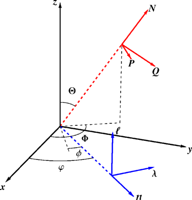
Figure 1: Definition of angles and polarization vectors. $\bm{N}$ points towards the observer, whose spherical coordinates are $(\Theta,\Phi)$, with $\Theta=\pi/2$ corresponding to the orbital plane of the binary; $\Theta$ is also the inclination of the orbit on the sky from the observer’s viewpoint. We define then $\bm{P}=-\bm{e}_{\Phi}$ and $\bm{Q}=\bm{e}_{\Theta}$. The ($\bm{n}$, $\bm{\lambda}$, $\bm{\ell}$) triad is displayed, $\varphi$ being the orbital phase, and $\phi\equiv\varphi-\Phi+\pi/2$ being the orbital phase relative to the direction of the ascending node of the orbit, which is also the direction of $\bm{P}$.

We now introduce two unit polarisation vectors $\bm{P}$ and $\bm{Q}$ forming with $\bm{N}$ an orthonormal triad, as indicated on Fig. 1. Representing the observers’s direction in spherical coordinates $(\Theta,\Phi)$, with $\Theta=\pi/2$ corresponding to the orbital plane of the binary, our choice for the polarization vectors (which is not unique) is $\bm{P}=-\bm{e}_{\Phi}$ and $\bm{Q}=\bm{e}_{\Theta}$, where $\bm{e}_{\Theta}=\partial\bm{N}/\partial\Theta$ and $\bm{e}_{\Phi}=\partial\bm{N}/(\sin\Theta\partial\Phi)$ are the standard transverse basis vectors of spherical coordinates. With respect to the polarization vectors $\bm{P}$ and $\bm{Q}$, the two polarization states are

$$h_{+} =\frac{1}{2}\left(P_{i}P_{j}-Q_{i}Q_{j}\right)h_{ij}^{\text{TT}}\,,$$ (12a)

$$h_{\times} =\frac{1}{2}\left(P_{i}Q_{j}+P_{j}Q_{i}\right)h_{ij}^{\text{TT}}\,.$$ (12b)

We shall henceforth pose $h\equiv h_{+}-\mathrm{i}h_{\times}$. For quasi-circular orbits the complex wave-amplitude $h$ will be a function of the orbital phase $\varphi=\int\omega\,\mathrm{d}t$ and of the spherical angles $(\Theta,\Phi)$ associated with $\bm{N}$. Next, we apply a decomposition in terms of spin-weighted spherical harmonics $Y^{\ell m}_{-2}(\Theta,\Phi)$. This yields the definition of the spherical modes $h^{\ell m}$ of the waveform as

$$h=\sum^{+\infty}_{\ell=2}\sum^{\ell}_{m=-\ell}h^{\ell m}\,Y^{\ell m}_{-2}(\Theta,\Phi)\,.$$ (13)

From the orthogonality properties of the $Y^{\ell m}_{-2}$’s, the separate modes $h^{\ell m}$ are extracted from $h$ by the surface integral (with solid angle element $\mathrm{d}^{2}\Omega=\sin\Theta\mathrm{d}\Theta\mathrm{d}\Phi$)

$$h^{\ell m}=\int\mathrm{d}^{2}\Omega\,h\,\overline{Y}^{\,\ell m}_{-2}(\Theta,\Phi)\,,$$ (14)

where the overbar means the complex conjugation. We can thus insert the waveform decomposition (11) in terms of STF radiative moments and perform the angular integration, to obtain

$$h^{\ell m}=-\frac{G}{\sqrt{2}\,R\,c^{\ell+2}}\left[U^{\ell m}-\frac{\mathrm{i}}{c}V^{\ell m}\right]\,,$$ (15)

where $U^{\ell m}$ and $V^{\ell m}$ are the radiative mass and current moments in standard (non-STF) form Th80 ; K08 , related to the STF radiative moments by

$$U^{\ell m} =\frac{4}{\ell!}\,\sqrt{\frac{(\ell+1)(\ell+2)}{2\ell(\ell-1)}}\,\alpha_{L}^{\ell m}\,U_{L}\,,$$ (16a)

$$V^{\ell m} =-\frac{8}{\ell!}\,\sqrt{\frac{\ell(\ell+2)}{2(\ell+1)(\ell-1)}}\,\alpha_{L}^{\ell m}\,V_{L}\,.$$ (16b)

Here we have introduced the tensor $\alpha_{L}^{\ell m}$ defined by the decomposition of the STF product of $\ell$ unit vectors $\bm{N}$, i.e. $\hat{N}_{L}$ in our notation, into ordinary spherical harmonics, namely

$$\hat{N}_{L}=\sum_{m=-\ell}^{\ell}\alpha_{L}^{\ell m}\,Y^{\ell m}(\Theta,\Phi)\,.$$ (17)

III.2 Mode separation for planar binaries

Let us now show that for planar binaries, the mode $h^{\ell m}$ is in fact entirely given by the “mass” contribution [first term in (15)] when $\ell+m$ is even, and by the “current” contribution [second term in (15)] when $\ell+m$ is odd. Notice that this is valid in general for non-spinning binaries, regardless of the orbit being quasi-circular or elliptical, or for spinning binaries with spins aligned or anti-aligned with the orbital angular momentum. The important point is only that the black holes must be non-precessing so that the motion is planar. This mode separation has been already used in Ref. K08 , but we explain here how to deduce it from an argument of parity invariance. If an observer with space-coordinates $\bm{X}$ in a spatial grid $\{X^{i}\}$ looks at the gravitational-wave signal at a given time $T$, he finds that the source particles lie at some positions $\bm{y}_{A}$ and possess certain velocities $\bm{v}_{A}$, for $A=1,2$. Now, a second observer located at $\bm{X}^{\prime}=-\bm{X}$ and looking at a parity-reversed system with positions $\bm{y}^{\prime}_{A}=-\bm{y}_{A}$ and velocities $\bm{v}^{\prime}_{A}=-\bm{v}_{A}$ must observe the same waveform $h_{ij}^{\text{TT}}$, by parity invariance of the Einstein field equations. This translates into:

$$h^{\text{TT}}_{ij}(-\bm{X},T;-\bm{y}_{A},-\bm{v}_{A})=h^{\text{TT}}_{ij}(\bm{X},T;\bm{y}_{A},\bm{v}_{A})\,.$$ (18)

Because the multipolar decomposition (11) is unique, this result allows us to recover the basic built-in parity properties of the mass and current moments $U_{L}$ and $V_{L}$, regarded as functionals of the matter variables $\bm{y}_{A}$, $\bm{v}_{A}$:

$$U_{L}(T;-\bm{y}_{A},-\bm{v}_{A})=(-1)^{\ell}\,U_{L}(T;\bm{y}_{A},\bm{v}_{A})\,,$$ (19a)

$$V_{L}(T;-\bm{y}_{A},-\bm{v}_{A})=(-1)^{\ell+1}\,V_{L}(T;\bm{y}_{A},\bm{v}_{A})\,.$$ (19b)

To see how Eq. (18) reflects on the two polarizations, we remark that the polarization vector $\bm{P}=\bm{N}\times\bm{\ell}/|\bm{N}\times\bm{\ell}|$ transforms as $\bm{P}^{\prime}=-\bm{P}$, while $\bm{Q}=\bm{N}\times\bm{P}$ is clearly invariant, due to the fact that $\bm{\ell}$ is itself invariant and $\bm{N}^{\prime}=-\bm{N}$. Those considerations applied to the complex polarization $h=h_{+}-\mathrm{i}h_{\times}$, with the definition (12) for $h_{+}$ and $h_{\times}$, show that, in the center-of-mass frame

$$h(-\bm{X},T;-\bm{x},-\bm{v})=\overline{h}(\bm{X},T;\bm{x},\bm{v})\,,$$ (20)

where $\bm{x}=\bm{y}_{1}-\bm{y}_{2}$ and $\bm{v}=\mathrm{d}\bm{x}/\mathrm{d}t$.

For planar motions, it is particularly convenient to rewrite the previous relations in the spherical coordinates associated with the frame $\{X^{i}\}$. The triad $\{\bm{N},\bm{P},\bm{Q}\}$ is specified by the inclination $\Theta$ and azimuthal angle $\Phi$ of the unit vector $\bm{N}$. Similarly, the mass-point location is determined by the pair of angles $(\theta=\pi/2,\varphi)$, where $\varphi$ is the orbital phase. The counterparts of those quantities for the reversed observer are $\Theta^{\prime}=\pi-\Theta$, $\Phi^{\prime}=\Phi+\pi$, $\theta^{\prime}=\pi/2$ and $\varphi^{\prime}=\varphi+\pi$. Note that the components of the relative position $\bm{x}$ and velocity $\bm{v}$ are solely functions of the azimuthal phase $\varphi$ on the trajectory $r=r(\varphi)$. Now as is clear from the geometry of the planar binary, the invariance under rotation implies that $h(R,T,\Theta,\Phi,\varphi)$ depends on $\Phi$ and $\varphi$ only through their difference $\varphi-\Phi$. Hence we define as a convenient phase variable $\phi\equiv\varphi-\Phi+\pi/2$, which is actually the orbital phase whose origin is chosen to be the direction of the ascending node $\bm{P}$ (see Fig. 1). We shall regard $h$ as a function of $\Theta$ and $\phi$, denoted by $h(\Theta,\phi)$ hitherto, ignoring dependences in $R$, $T$ since they do not play a role here. Putting those results together, we arrive at the important identity

$$h(\pi-\Theta,\phi)=\overline{h}(\Theta,\phi)\,.$$ (21)

Inserting the definition (14) of $h^{\ell m}$ into both sides of the latter equation and noticing GMNRS67 that $\overline{Y}^{\ell m}_{-2}(\pi-\Theta,\Phi+\pi)=(-1)^{m+\ell}Y^{\ell\,-m}_{-2}(\Theta,\Phi)$, we conclude from the uniqueness of the decomposition in spin-weighted spherical harmonics that

$$h^{\ell m}(\varphi)=(-1)^{\ell+m}\,\overline{h}^{\ell,-m}(\varphi+\pi)\,.$$ (22)

The known dependence of the mode on the azimuthal angle, $h^{\ell m}(\varphi)\propto e^{-\mathrm{i}m\varphi}$, then shows that

$$h^{\ell m}(\varphi)=(-1)^{\ell}\,\overline{h}^{\ell,-m}(\varphi)\,.$$ (23)

In the end, we substitute for $h^{\ell m}$ its expression (15) in the equality above. The tensor $\alpha_{L}^{\ell m}$ introduced in Eqs. (16) satisfies $\overline{\alpha}_{L}^{\ell,-m}=(-1)^{m}\,\alpha_{L}^{\ell m}$, which implies that the multipolar coefficients $U^{\ell m}$ and $V^{\ell m}$ satisfy themselves the relations $\overline{U}^{\ell,-m}=(-1)^{m}\,U^{\ell m}$ and $\overline{V}^{\ell,-m}=(-1)^{m}\,V^{\ell m}$. Finally, we find that these multipole coefficients must be such that $U^{\ell m}=(-1)^{\ell+m}\,U^{\ell m}$ and $V^{\ell m}=(-1)^{\ell+m+1}\,V^{\ell m}$, hence we have necessarily $U^{\ell m}=0$ when $\ell+m$ is odd, and $V^{\ell m}=0$ when $\ell+m$ is even. We therefore conclude that there is no mixture between the mass-type and current-type contributions to the modes, in the sense that

$$h^{\ell m} =-\frac{G}{\sqrt{2}Rc^{\ell+2}}\,U^{\ell m}\qquad\text{when $\ell+m$ is even}\,,$$ (24a)

$$h^{\ell m} =\frac{G}{\sqrt{2}Rc^{\ell+3}}\,\mathrm{i}\,V^{\ell m}~{}\qquad\text{when $\ell+m$ is odd}\,.$$ (24b)

Let us stress again that this result holds only when the orbit stays planar and, in particular, does not apply to precessing binaries. However, it is valid for quasi-circular as well as elliptical orbits.

IV Expression of the dominant quadrupole mode

In the following sections, we shall compute the dominant quadrupole mode $(\ell,m)=(2,2)$ at 3.5PN order. From the results (24), the mode $h^{22}$ depends only on the radiative mass-type quadrupole moment $U_{ij}$,

$$h^{22}=-\frac{G}{\sqrt{2}Rc^{4}}\,U^{22}=-\frac{\sqrt{6}G}{Rc^{4}}\,\alpha^{22}_{ij}\,U_{ij}\,.$$ (25)

Following the multipolar-post-Minkowskian (MPM) formalism BD86 ; BD92 ; B98quad ; B98tail ; B98mult , we shall express the radiative quadrupole moment $U_{ij}$ in terms successively of canonical moments $\{M_{L},S_{L}\}$ and then source moments $\{I_{L},J_{L},W_{L},X_{L},Y_{L},Z_{L}\}$ for general sources at 3.5PN order. Among the source moments, $\{I_{L},J_{L}\}$ are the most important ones because they arise at Newtonian order, while $\{W_{L},X_{L},Y_{L},Z_{L}\}$, which are called the gauge moments, induce corrections starting at high 2.5PN order.

Using the “selection rules” developed in Paper I, we can identify all types of terms to be computed up to quadratic order (which is sufficient for our purpose). Let $\ell_{\text{max}}[A_{J},B_{K}]$ be the maximum multipolar order beyond which $U_{L}$ cannot contain products of the two multipole moments $A_{J}$ and $B_{K}$ or their time derivatives (or possibly time anti-derivatives), at the 3.5PN level. Here $A_{J}$ and $B_{K}$ can be any moments chosen among the set of source moments $\{I_{L},J_{L},W_{L},X_{L},Y_{L},Z_{L}\}$. Thus when $\ell>\ell_{\text{max}}[A_{J},B_{K}]$ any term in $U_{L}$ constructed with the product of moments $A_{J}$ and $B_{K}$ has a post-Newtonian order strictly higher than 3.5PN and is negligible here. On the other hand when $\ell_{\text{max}}[A_{J},B_{K}]<2$, the corresponding interaction is not allowed to enter the quadrupole moment $U_{ij}$ which has $\ell=2$. When $\ell_{\text{max}}[A_{J},B_{K}]\geqslant 2$, it is equal to the number of (free or dummy) indices to be shared between: (i) $A_{J}$ and $B_{K}$ if both moments are of the same parity, i.e. $j+k=\ell_{\text{max}}[A_{J},B_{K}]$, or (ii) $A_{aJ-1}$, $B_{bK-1}$ and $\varepsilon_{iab}$ (with contractions on indices $a$ and $b$) if both moments are of different parity, i.e. $j+k=\ell_{\text{max}}[A_{J},B_{K}]+1$. The values of $\ell_{\text{max}}[A_{J},B_{K}]$ larger than or equal to 2 are listed in Table 1 for the various possible choices of $A_{J}$ and $B_{K}$. Take for instance the case of $I_{J}$ and $I_{K}$. By dimensionality we can add the powers of $1/c$ and find that this term is necessarily of the type ($p$ and $q$ being the number of time derivatives)

$$U_{L}\sim\frac{G}{c^{j+k+3-\ell}}\,I_{J}^{(p)}I_{K}^{(q)}\,.$$ (26)

The contribution of this term in the waveform (11) is easily seen to be of post-Newtonian order $\mathcal{O}(1/c^{j+k+1})$ and hence we require $j+k=6$ for a 3.5PN term. On the other hand, we have said that $\ell_{\text{max}}=j+k$ in this case, hence we have $\ell_{\text{max}}=6$ in Table 1 for a contribution like (26). Similar selection rules can be made for the radiative current moment $V_{L}$ but here we need only to compute the mass quadrupole moment. From Table 1, it is straightforward to obtain the set of quadratic interactions contributing to $U_{ij}$ within our accuracy. No new cubic interaction (between three source moments), besides the already known 3PN tail-of-tail term, enters the mass quadrupole $U_{ij}$ at the 3.5PN order.

$A_{J}$	$B_{K}$
	$I_{K}$	$J_{K}$	$W_{K}$	$X_{K}$	$Y_{K}$	$Z_{K}$
$I_{J}$	6	4	4	2	4	2
$J_{J}$	4	4	2	–	2	2
$W_{J}$	4	2	2	–	2	–
$X_{J}$	2	–	–	–	–	–
$Y_{J}$	4	2	2	–	2	–
$Z_{J}$	2	2	–	–	–	–

Table 1: Values of $\ell_{\text{max}}[A_{J},B_{K}]$ at the 3.5PN order for the various possible choices of $A_{J}$ and $B_{K}$. Because factors may always be reordered in products, we have $\ell_{\text{max}}[A_{J},B_{K}]=\ell_{\text{max}}[B_{J},A_{K}]$ and the table is trivially symmetric.

The long calculation following the MPM algorithm BD86 (in the slightly modified version of Ref. B98quad ), is implemented in a systematic way by means of the tensor package xTensor developed for Mathematica xtensor , and yields various types of terms:

$$U_{ij}=U^{\text{inst}}_{ij}+U^{\text{tail}}_{ij}+U^{\text{mem}}_{ij}\,.$$ (27)

In a first stage we express each of the different pieces by means of the canonical moments $\{M_{L},S_{L}\}$. The instantaneous piece up to 3.5PN order is

$$U_{ij}^{\text{inst}} =M^{(2)}_{ij}$$

$$+\frac{G}{c^{5}}\biggl{[}\frac{1}{7}M^{(5)}_{a\langle i}M_{j\rangle a}-\frac{5}{7}M^{(4)}_{a\langle i}M^{(1)}_{j\rangle a}-\frac{2}{7}M^{(3)}_{a\langle i}M^{(2)}_{j\rangle a}+\frac{1}{3}\varepsilon_{ab\langle i}M^{(4)}_{j\rangle a}S_{b}\biggr{]}$$

$$+\frac{G}{c^{7}}\bigg{[}-\frac{64}{63}S^{(2)}_{a{\langle i}}S^{(3)}_{{j\rangle}a}+\frac{1957}{3024}M^{(3)}_{ijab}M^{(4)}_{ab}+\frac{5}{2268}M^{(3)}_{ab{\langle i}}M^{(4)}_{{j\rangle}ab}+\frac{19}{648}M^{(3)}_{ab}M^{(4)}_{ijab}$$

$$\qquad\quad+\frac{16}{63}S^{(1)}_{a{\langle i}}S^{(4)}_{{j\rangle}a}+\frac{1685}{1008}M^{(2)}_{ijab}M^{(5)}_{ab}+\frac{5}{126}M^{(2)}_{ab{\langle i}}M^{(5)}_{{j\rangle}ab}-\frac{5}{756}M^{(2)}_{ab}M^{(5)}_{ijab}$$

$$\qquad\quad+\frac{80}{63}S_{a{\langle i}}S^{(5)}_{{j\rangle}a}+\frac{5}{42}S_{a}S^{(5)}_{ija}+\frac{41}{28}M^{(1)}_{ijab}M^{(6)}_{ab}+\frac{5}{189}M^{(1)}_{ab{\langle i}}M^{(6)}_{{j\rangle}ab}$$

$$\qquad\quad+\frac{1}{432}M^{(1)}_{ab}M^{(6)}_{ijab}+\frac{91}{216}M_{ijab}M^{(7)}_{ab}-\frac{5}{252}M_{ab{\langle i}}M^{(7)}_{{j\rangle}ab}-\frac{1}{432}M_{ab}M^{(7)}_{ijab}$$

$$\qquad\quad+\varepsilon_{ac{\langle i}}\Big{(}\frac{32}{189}M^{(3)}_{{j\rangle}bc}S^{(3)}_{ab}-\frac{1}{6}M^{(3)}_{ab}S^{(3)}_{{j\rangle}bc}+\frac{3}{56}S^{(2)}_{{j\rangle}bc}M^{(4)}_{ab}+\frac{10}{189}S^{(2)}_{ab}M^{(4)}_{{j\rangle}bc}$$

$$\qquad\quad+\frac{65}{189}M^{(2)}_{{j\rangle}bc}S^{(4)}_{ab}+\frac{1}{28}M^{(2)}_{ab}S^{(4)}_{{j\rangle}bc}+\frac{187}{168}S^{(1)}_{{j\rangle}bc}M^{(5)}_{ab}-\frac{1}{189}S^{(1)}_{ab}M^{(5)}_{{j\rangle}bc}$$

$$\qquad\quad-\frac{5}{189}M^{(1)}_{{j\rangle}bc}S^{(5)}_{ab}+\frac{1}{24}M^{(1)}_{ab}S^{(5)}_{{j\rangle}bc}+\frac{65}{84}S_{{j\rangle}bc}M^{(6)}_{ab}+\frac{1}{189}S_{ab}M^{(6)}_{{j\rangle}bc}$$

$$\qquad\quad-\frac{10}{63}M_{{j\rangle}bc}S^{(6)}_{ab}+\frac{1}{168}M_{ab}S^{(6)}_{{j\rangle}bc}\Big{)}\bigg{]}\,,$$ (28)

where the angle brackets $\langle\,\rangle$ around indices $i$ and $j$ denote their STF projection (for convenience we do not indicate the neglected remainder $\mathcal{O}(1/c^{8})$). The hereditary tail integrals involve the dominant tail term at 1.5PN order BD92 and the tail-of-tail term at 3PN order B98tail :

$$U^{\text{tail}}_{ij} =\frac{2GM}{c^{3}}\int_{-\infty}^{T_{R}}\mathrm{d}\tau\left[\ln\left(\frac{T_{R}-\tau}{2\tau_{0}}\right)+\frac{11}{12}\right]M^{(4)}_{ij}(\tau)$$

$$+2\left(\frac{GM}{c^{3}}\right)^{2}\int_{-\infty}^{T_{R}}\mathrm{d}\tau\left[\ln^{2}\left(\frac{T_{R}-\tau}{2\tau_{0}}\right)+\frac{57}{70}\ln\left(\frac{T_{R}-\tau}{2\tau_{0}}\right)+\frac{124627}{44100}\right]M^{(5)}_{ij}(\tau)\,,$$ (29)

where $\tau_{0}$ denotes an arbitrary constant which will enter in fine into some unphysical frequency scale (40) in the waveform. The memory-type hereditary integrals, which constitute the third piece in Eq. (27), contribute here at orders 2.5PN and 3.5PN. Our expression extends the classic works on the dominant 2.5PN non-linear memory effect BD92 ; Chr91 ; Th92 ; WW91 ; B98quad , and is in agreement with the recent computation of the non-linear memory up to any post-Newtonian order in Refs. F09 ; F11 . We have

$$U_{ij}^{\text{mem}} =\frac{G}{c^{5}}\biggl{[}-\frac{2}{7}\int_{-\infty}^{T_{R}}\mathrm{d}\tau\,M^{(3)}_{a\langle i}(\tau)\,M^{(3)}_{j\rangle a}(\tau)\biggr{]}$$

$$+\frac{G}{c^{7}}\bigg{[}-\frac{32}{63}\int_{-\infty}^{T_{R}}\mathrm{d}\tau\,S^{(3)}_{a{\langle i}}(\tau)\,S^{(3)}_{{j\rangle}a}(\tau)-\frac{5}{756}\int_{-\infty}^{T_{R}}\mathrm{d}\tau\,M^{(4)}_{ab}(\tau)\,M^{(4)}_{ijab}(\tau)$$

$$\qquad\quad-\frac{20}{189}\,\varepsilon_{ab{\langle i}}\int_{-\infty}^{T_{R}}\mathrm{d}\tau\,S^{(3)}_{ac}(\tau)\,M^{(4)}_{{j\rangle}bc}(\tau)+\frac{5}{42}\,\varepsilon_{ab{\langle i}}\int_{-\infty}^{T_{R}}\mathrm{d}\tau\,M^{(3)}_{ac}(\tau)\,S^{(4)}_{{j\rangle}bc}(\tau)\biggr{]}\,.$$ (30)

In a second stage of the general formalism, we must express the canonical moments $\{M_{L},S_{L}\}$ in terms of the six types of source moments $\{I_{L},J_{L},W_{L},X_{L},Y_{L},Z_{L}\}$. For the present computation we need only to relate the canonical quadrupole moment $M_{ij}$ to the corresponding source quadrupole moment $I_{ij}$ up to 3.5PN order. We obtain

$$M_{ij} =I_{ij}+\frac{4G}{c^{5}}\left[W^{(2)}I_{ij}-W^{(1)}I_{ij}^{(1)}\right]$$

$$+\frac{4G}{c^{7}}\biggl{[}\frac{4}{7}W^{(1)}_{a{\langle i}}I^{(3)}_{{j\rangle}a}+\frac{6}{7}W_{a{\langle i}}I^{(4)}_{{j\rangle}a}-\frac{1}{7}I_{a{\langle i}}Y^{(3)}_{{j\rangle}a}-Y_{a{\langle i}}I^{(3)}_{{j\rangle}a}-2XI^{(3)}_{ij}-\frac{5}{21}I_{ija}W^{(4)}_{a}$$

$$\qquad\quad+\frac{1}{63}I^{(1)}_{ija}W^{(3)}_{a}-\frac{25}{21}I_{ija}Y^{(3)}_{a}-\frac{22}{63}I^{(1)}_{ija}Y^{(2)}_{a}+\frac{5}{63}Y^{(1)}_{a}I^{(2)}_{ija}+2W_{ij}W^{(3)}$$

$$\qquad\quad+2W_{ij}^{(1)}W^{(2)}-\frac{4}{3}W_{{\langle i}}W_{{j\rangle}}^{(3)}+2Y_{ij}W^{(2)}-4W_{\langle i}Y^{(2)}_{j\rangle}$$

$$\qquad\quad+\varepsilon_{ab{\langle i}}\biggl{(}\frac{1}{3}I_{{j\rangle}a}Z^{(3)}_{b}+\frac{4}{9}J_{{j\rangle}a}W^{(3)}_{b}-\frac{4}{9}J_{{j\rangle}a}Y^{(2)}_{b}+\frac{8}{9}J^{(1)}_{{j\rangle}a}Y^{(1)}_{b}+Z_{a}I^{(3)}_{{j\rangle}b}\biggr{)}\biggr{]}\,.$$ (31)

The current quadrupole canonical moment $S_{ij}$ and mass octupole canonical moment $M_{ijk}$ agree with the corresponding source moments up to 2PN order, and for this computation it is sufficient to replace these by their source counterparts.

V Source multipole moments of compact binaries

We now feed the previous expression of the radiative quadrupole moment $U_{ij}$ with explicit results for the source moments in the case of non-spinning compact binaries on quasi-circular orbits. The general formulas for the six sets of source moments $\{I_{L},J_{L},W_{L},X_{L},Y_{L},Z_{L}\}$ as explicit integrals over the matter distribution in the source and the gravitational field were obtained in Ref. B98mult . The mass-type source moments expressed in terms of elementary retarded potentials up to 3.5PN order are given by Eqs. (3.3)–(3.6) of Ref. BI04mult . Reducing the latter source quadrupole moment $I_{ij}$ for compact binaries, in the frame of the center-of-mass and for quasi-circular orbits, yields

$$I_{ij}=\nu\,m\,\left(\mathcal{A}\,x^{\langle i}x^{j\rangle}+\frac{r^{2}}{c^{2}}\,\mathcal{B}\,v^{\langle i}v^{j\rangle}+\frac{48}{7}\frac{G^{2}m^{2}\nu}{c^{5}r}\,\mathcal{C}_{\text{RR}}\,x^{\langle i}v^{j\rangle}\right)+\mathcal{O}\left(\frac{1}{c^{8}}\right)\,,$$ (32)

where $x^{i}$ is the orbital separation and $v^{i}=\mathrm{d}x^{i}/\mathrm{d}t$ is the relative velocity. Resorting also to the post-Newtonian parameter $\gamma$ defined by Eq. (3), the “conservative” coefficients $\mathcal{A}$ and $\mathcal{B}$ in (32) read

$$\mathcal{A} =1+\gamma\left(-\frac{1}{42}-\frac{13}{14}\nu\right)+\gamma^{2}\left(-\frac{461}{1512}-\frac{18395}{1512}\nu-\frac{241}{1512}\nu^{2}\right)$$

$$~{}~{}+\gamma^{3}\left(\frac{395899}{13200}-\frac{428}{105}\ln\left(\frac{r}{r_{0}}\right)+\left[\frac{3304319}{166320}-\frac{44}{3}\ln\left(\frac{r}{r^{\prime}_{0}}\right)\right]\nu\right.$$

$$~{}~{}\qquad+\left.\frac{162539}{16632}\nu^{2}+\frac{2351}{33264}\nu^{3}\right)\,,$$ (33a)

$$\mathcal{B} =\frac{11}{21}-\frac{11}{7}\nu+\gamma\left(\frac{1607}{378}-\frac{1681}{378}\nu+\frac{229}{378}\nu^{2}\right)$$

$$~{}~{}+\gamma^{2}\left(-\frac{357761}{19800}+\frac{428}{105}\ln\left(\frac{r}{r_{0}}\right)-\frac{92339}{5544}\nu+\frac{35759}{924}\nu^{2}+\frac{457}{5544}\nu^{3}\right)\,.$$ (33b)

The results at 3PN order were already known BIJ02 ; BI04mult . Note the appearance at 3PN order of two arbitrary scales: the first one is given by $r_{0}=c\tau_{0}$, where $\tau_{0}$ is the same scale as in the tail integrals (IV); the second one is a Hadamard regularization scale $r^{\prime}_{0}$ due to the presence of the point mass singularities. The scale $r_{0}$ is associated with an irrelevant choice of the origin of time in the radiative zone, whereas the scale $r^{\prime}_{0}$ will disappear from our final results, being cancelled by the corresponding $r^{\prime}_{0}$ in the equations of motion; see Eq. (II). The new correction term at 3.5PN order only affects, for circular orbits, the “radiation reaction” coefficient $\mathcal{C}_{\text{RR}}$ which is found to be

$$\mathcal{C}_{\text{RR}}=1+\gamma\left(-\frac{256}{135}-\frac{1532}{405}\nu\right)\,.$$ (34)

We give the result for the complete 3.5PN mass quadrupole moment in the case of generic orbits reduced to the center-of-mass frame in Appendix A.

In addition to the 3.5PN mass quadrupole $I_{ij}$ we will also need the expression of the mass monopole or ADM mass $M$ (notice that $I\equiv M$) up to 2PN order since it is required in the computation of the tail terms (IV). We have, for circular orbits:

$$M=m\biggl{[}1-\frac{\nu}{2}\gamma+\frac{\nu}{8}\bigl{(}7-\nu\bigr{)}\gamma^{2}\biggr{]}+\mathcal{O}\left(\frac{1}{c^{5}}\right)\,.$$ (35)

Furthermore the current dipole moment $J_{i}$ is required up to 1PN order, since it appears in the 2.5PN term of Eq. (IV) (recall that $S_{i}=J_{i}$ in our approximation):

$$J_{i}=\nu\,m\,\varepsilon_{ijk}\,x^{j}v^{k}\left[1+\gamma\left(\frac{7}{2}-\frac{1}{2}\nu\right)\right]+\mathcal{O}\left(\frac{1}{c^{4}}\right)\,.$$ (36)

The other source moments $I_{L}$ and $J_{L}$ are required at Newtonian order only, and at that order we have the following general formulas, valid for all multipolar indices $\ell\geqslant 2$:

$$I_{L} =\nu\,m\,s_{\ell}(\nu)\,\hat{x}_{L}+\mathcal{O}\left(\frac{1}{c^{2}}\right)\,,$$ (37a)

$$J_{L} =\nu\,m\,s_{\ell+1}(\nu)\,L_{\langle i_{\ell}}\hat{x}_{L-1\rangle}+\mathcal{O}\left(\frac{1}{c^{2}}\right)\,.$$ (37b)

Here we denote $L_{i}=\varepsilon_{ijk}\,x^{j}v^{k}$ and $s_{\ell}(\nu)=X_{2}^{\ell-1}+(-1)^{\ell}X_{1}^{\ell-1}$, with $X_{1}=\frac{m_{1}}{m}=\frac{1}{2}(1+\Delta)$ and $X_{2}=\frac{m_{2}}{m}=\frac{1}{2}(1-\Delta)$ where $\Delta=\frac{m_{1}-m_{2}}{m}=\pm\sqrt{1-4\nu}$; see also Footnote $24$ of Paper I for an alternative expression of the function $s_{\ell}(\nu)$.

Among the required gauge-type source moments $\{W_{L},X_{L},Y_{L},Z_{L}\}$, the only one which is to be controlled at 1PN order is the monopole $W$, since it enters the 2.5PN term of Eq. (IV). However it turns out to be zero for quasi-circular orbits. The other needed moments are merely Newtonian. Their full list is as follows:

$$W =0+\mathcal{O}\left(\frac{1}{c^{4}}\right)\,,$$ (38a)

$$W_{i} =\frac{1}{10}m\,\nu\,\Delta\,r^{2}\,v^{i}+\mathcal{O}\left(\frac{1}{c^{2}}\right)\,,$$ (38b)

$$W_{ij} =-\frac{2}{21}m\,\nu\bigl{(}1-3\nu\bigr{)}r^{2}x^{\langle i}v^{j\rangle}+\mathcal{O}\left(\frac{1}{c^{2}}\right)\,,$$ (38c)

$$X =\frac{1}{12}Gm^{2}r\,\nu\,\bigl{(}-1+\nu\bigr{)}+\mathcal{O}\left(\frac{1}{c^{2}}\right)\,,$$ (38d)

$$Y_{i} =\frac{Gm^{2}\nu}{5r}\Delta\,x^{i}+\mathcal{O}\left(\frac{1}{c^{2}}\right)\,,$$ (38e)

$$Y_{ij} =\frac{1}{14}\frac{Gm^{2}\nu}{r}\bigl{(}-3+16\nu\bigr{)}x^{\langle i}x^{j\rangle}-\frac{2}{7}m\,\nu\bigl{(}1-3\nu\bigr{)}r^{2}\,v^{\langle i}v^{j\rangle}+\mathcal{O}\left(\frac{1}{c^{2}}\right)\,,$$ (38f)

$$Z_{i} =0+\mathcal{O}\left(\frac{1}{c^{2}}\right)\,.$$ (38g)

Finally, when computing the waveform, we need the multiple time derivatives of all these moments; they are computed by order reduction using the acceleration for quasi-circular orbits given at 3.5PN order by Eq. (9). Furthermore, we need to perform many scalar products between the velocity and the polarization vectors $(\bm{N},\bm{P},\bm{Q})$; these are computed using the 3.5PN expression of the velocity as given by Eq. (10). Note also that the (tails and non-linear memory) hereditary terms given by Eqs. (IV) and (IV) are treated by exactly the same method as in Paper I.

VI Dominant quadrupolar mode at 3.5PN order

We shall now perform a change of phase variable, from the actual orbital phase related to the orbital frequency by $\varphi=\int\omega\mathrm{d}t$, to a new phase variable $\psi$, defined in such a way that it absorbs most of the logarithmic contributions in the frequency coming from the tail terms. Extending Refs. BIWW96 ; ABIQ04 ; BFIS08 , we find that the new phase variable takes remarkably the same expression as the one used in Paper I:

$$\psi=\varphi-\frac{2GM\omega}{c^{3}}\ln\left(\frac{\omega}{\omega_{0}}\right)\,.$$ (39)

The 2PN corrections in the ADM mass $M$, as given by Eq. (35), are exactly the ones needed for the logarithmic cancellations at our extended 3.5PN order. Here $\omega_{0}$ is a constant frequency scale related to the constant $\tau_{0}$ appearing in the tail integrals (IV) by

$$\omega_{0}=\frac{e^{\frac{11}{12}-\gamma_{\text{E}}}}{4\tau_{0}}\,,$$ (40)

with $\gamma_{\text{E}}=0.577\cdots$ denoting the Euler constant. It is known BIWW96 that this frequency scale is irrelevant: a rescaling of $\omega_{0}$ is indeed equivalent to a shift of the binary’s instant of coalescence, which can be absorbed into a redefinition of the origin of time in the radiation zone. Physically, the logarithmic term in Eq. (39) expresses the fact that the tails induce a small delay in the arrival time of gravitational waves. When viewed as a modulation of the orbital phase as in (39), this term represents in fact a very small correction to this phase, being of order 4PN when compared to the dominant phase evolution which is at the “inverse” of 2.5PN order (i.e. at order $c^{+5}$), and is negligible with the present accuracy.

Replacing $\varphi$ in terms of the new phase variable $\psi$, we perform the appropriate Taylor expansion of the waveform and apply the mode decomposition (13). We also use the fact that, from the planar geometry of the problem, $h=h_{+}-\mathrm{i}h_{\times}$ depends only on the inclination angle $\Theta$ and the difference $\psi-\Phi$ between the “absolute” phase $\psi$ and the azimuth $\Phi$ of the vector $\bm{N}$ (see also Sec. III and Fig. 1). For instance, like in Eq. (21) but with $\psi$ playing now the role of $\varphi$, we can introduce the phase $\tilde{\phi}=\psi-\Phi+\pi/2$ defined relatively to the direction of the ascending node $\bm{P}$. Choosing the latter phase as integration variable instead of $\Phi$, and using the known dependence of the spherical harmonics on the angle $\tilde{\phi}$, we obtain

$$h^{\ell m}(\psi)=(-\mathrm{i})^{m}\,e^{-\mathrm{i}m\,\psi}\int\mathrm{d}\Omega\,h(\Theta,\tilde{\phi})\,Y^{\,\ell m}_{-2}(\Theta,\tilde{\phi})\,,$$ (41)

exhibiting the azimuthal factor $e^{-\mathrm{i}m\,\psi}$ appropriate for each mode. Alternatively, we may access directly a given $h^{\ell m}$ mode, once the requisite radiative multipole $U_{L}$ or $V_{L}$ known, by using the contraction formulas (16), which translate into (25) for $h^{22}$. Finally, to present our result we pose

$$h^{\ell m}=\frac{2G\,m\,\nu\,x}{R\,c^{2}}\,\sqrt{\frac{16\pi}{5}}\,H^{\ell m}\,e^{-\mathrm{i}m\,\psi}\,,$$ (42)

and express it entirely with the help of the gauge invariant post-Newtonian parameter $x$ related to the orbital frequency by Eq. (5). We find for the dominant $(2,2)$ mode up to 3.5PN order (extending the 3PN result of Paper I for this mode):

$$H^{22} =1+x\left(-\frac{107}{42}+\frac{55}{42}\nu\right)+2\pi x^{3/2}+x^{2}\left(-\frac{2173}{1512}-\frac{1069}{216}\nu+\frac{2047}{1512}\nu^{2}\right)$$

$$+x^{5/2}\left(-\frac{107\pi}{21}-24\,\mathrm{i}\,\nu+\frac{34\pi}{21}\nu\right)+x^{3}\bigg{(}\frac{27027409}{646800}-\frac{856}{105}\,\gamma_{\text{E}}+\frac{428\,\mathrm{i}\,\pi}{105}+\frac{2\pi^{2}}{3}$$

$$\qquad+\left(-\frac{278185}{33264}+\frac{41\pi^{2}}{96}\right)\nu-\frac{20261}{2772}\nu^{2}+\frac{114635}{99792}\nu^{3}-\frac{428}{105}\ln(16x)\bigg{)}$$

$$+x^{7/2}\left(-\frac{2173\pi}{756}+\left(-\frac{2495\pi}{378}+\frac{14333\,\mathrm{i}}{162}\right)\nu+\left(\frac{40\pi}{27}-\frac{4066\,\mathrm{i}}{945}\right)\nu^{2}\right)\,.$$ (43)

We have verified that the above expression is in full agreement in the test mass limit where $\nu\to 0$, with the result of black-hole perturbation theory as reported in the Appendix B of Ref. TSasa94 or, in a form more suitable for comparison, in Eq. (4.9a) of Ref. FI10 .

As it is the dominant quadrupole $(2,2)$ mode that is determined with the best precision by numerical relativity, the 3.5PN result (VI) should become important for high-accuracy comparisons between numerical and analytical waveforms. See Paper I for all the other modes that contribute up to 3PN order. The completion of the remaining modes at 3.5PN order presents some new difficulties; in particular the $(2,1)$ mode necessitates the difficult extension of the current quadrupole moment $J_{ij}$ up to 3PN order. This is left for future work.

Appendix A 3.5PN mass quadrupole moment

We give our result for the complete source mass quadrupole $I_{ij}$ up to 3.5PN order, for general non-circular orbits, but reduced to the center-of-mass frame. Defining:

$$I_{ij} =\nu\,m\,\left[\left(\mathcal{A}-\frac{24}{7}\frac{G^{2}m^{2}\nu}{c^{5}r^{2}}\,\dot{r}\mathcal{A}_{\text{RR}}\right)\,x^{\langle i}x^{j\rangle}+\left(\frac{r^{2}}{c^{2}}\,\mathcal{B}+\frac{Gm\nu}{c^{5}}\,r\,\dot{r}\,\mathcal{B}_{\text{RR}}\right)v^{\langle i}v^{j\rangle}\right.$$

$$\left.\qquad\quad+2\left(\frac{r\dot{r}}{c^{2}}\,\mathcal{C}+\frac{24}{7}\frac{G^{2}m^{2}\nu}{c^{5}r}\mathcal{C}_{\text{RR}}\right)x^{\langle i}v^{j\rangle}\right]\,,$$ (44)

the expressions for the conservative parts $\mathcal{A}$, $\mathcal{B}$, and $\mathcal{C}$ read:

$$\mathcal{A} =1+\frac{1}{c^{2}}\left[v^{2}\,\left(\frac{29}{42}-\frac{29\,\nu}{14}\right)+\frac{G\,m}{r}\,\left(-\frac{5}{7}+\frac{8}{7}\,\nu\ \right)\right]$$

$$+\frac{1}{c^{4}}\left[v^{2}\,\frac{G\,m}{r}\,\left(\frac{2021}{756}-\frac{5947}{756}\,\nu-\frac{4883}{756}\,\nu^{2}\right)\right.$$

$$\qquad\left.+\left(\frac{G\,m}{r}\right)^{2}\,\left(-\frac{355}{252}-\frac{953}{126}\,\nu+\frac{337\,}{252}\,\nu^{2}\right)\right.$$

$$\qquad+\left.v^{4}\,\left(\frac{253}{504}-\frac{1835}{504}\,\nu+\frac{3545}{504}\,\nu^{2}\right)\right.$$

$$\qquad\left.+\dot{r}^{2}\,\frac{G\,m}{r}\,\left(-\frac{131}{756}+\frac{907}{756}\,\nu-\frac{1273}{756}\,\nu^{2}\right)\right]$$

$$+\frac{1}{c^{6}}\left[v^{6}\,\left(\frac{4561}{11088}-\frac{7993}{1584}\,\nu+\frac{117067}{5544}\,\nu^{2}-\frac{328663}{11088}\,\nu^{3}\right)\right.$$

$$\left.\qquad+v^{4}\,\frac{G\,m}{r}\,\left(\frac{307}{77}-\frac{94475}{4158}\,\nu+\frac{218411}{8316}\,\nu^{2}+\frac{299857}{8316}\,\nu^{3}\right)\right.$$

$$\qquad+\left(\frac{G\,m}{r}\right)^{3}\,\left(\frac{6285233}{207900}+\frac{15502}{385}\,\nu-\frac{3632}{693}\,\nu^{2}+\frac{13289}{8316}\,\nu^{3}\right.$$

$$\qquad\quad\left.-\frac{428}{105}\,\ln\left(\frac{r}{r_{0}}\right)-\frac{44}{3}\,\,\nu\,\ln\left(\frac{r}{r_{0}^{\prime}}\right)\right)$$

$$\qquad+{\dot{r}}^{2}\,\left(\frac{G\,m}{r}\right)^{2}\,\left(-\frac{8539}{20790}+\frac{52153}{4158}\,\nu-\frac{4652}{231}\,\nu^{2}-\frac{54121}{5544}\,\nu^{3}\right)\,$$

$$\qquad+{\dot{r}}^{4}\,\frac{G\,m}{r}\,\left(\frac{2}{99}-\frac{1745}{2772}\,\nu+\frac{16319}{5544}\,\nu^{2}-\frac{311\,}{99}\,\nu^{3}\right)\,$$

$$\qquad+v^{2}\,\left(\frac{G\,m}{r}\right)^{2}\,\left(\frac{187183}{83160}-\frac{605419}{16632}\,\nu+\frac{434909}{16632}\,\nu^{2}-\frac{37369}{2772}\,\nu^{3}\right)$$

$$\qquad+\left.v^{2}\,\frac{G\,m}{r}\,\,{\dot{r}}^{2}\,\left(-\frac{757}{5544}+\frac{5545}{8316}\,\nu-\frac{98311\,}{16632}\,\nu^{2}+\frac{153407}{8316}\,\nu^{3}\right)\right]\,,$$ (45a)

$$\mathcal{B} =\frac{11}{21}-\frac{11}{7}\,\nu$$

$$+\frac{1}{c^{2}}\left[\frac{Gm}{r}\,\left(\frac{106}{27}-\frac{335}{189}\,\nu-\frac{985}{189}\,\nu^{2}\right)\right.$$

$$\qquad\left.+\,v^{2}\,\left(\frac{41}{126}-\frac{337}{126}\,\nu+\frac{733}{126}\,\nu^{2}\right)+\dot{r}^{2}\,\left(\frac{5\,}{63}-\frac{25}{63}\,\nu+\frac{25}{63}\,\nu^{2}\right)\right]$$

$$+\frac{1}{c^{4}}\,\left[\,v^{4}\,\left(\frac{1369}{5544}-\frac{19351}{5544}\,\nu+\frac{45421}{2772}\,\nu^{2}-\frac{139999}{5544}\,\nu^{3}\right)\right.$$

$$\qquad+\left.\left(\frac{Gm}{r}\right)^{2}\,\left(-\frac{40716}{1925}-\frac{10762}{2079}\,\nu+\frac{62576}{2079}\,\nu^{2}-\frac{24314}{2079}\,\nu^{3}\right.\right.$$

$$\qquad\quad\left.\left.+\frac{428}{105}\,\ln\left(\frac{r}{r_{0}}\right)\right)\right.$$

$$\qquad+\dot{r}^{2}\,\frac{Gm}{r}\left(\frac{79}{77}-\frac{5807}{1386}\,\nu+\frac{515}{1386}\,\nu^{2}+\frac{8245}{693}\,\nu^{3}\right)$$

$$\qquad+v^{2}\,\frac{Gm}{r}\,\left(\frac{587}{154}-\frac{67933}{4158}\,\nu+\frac{25660}{2079}\,\nu^{2}+\frac{129781}{4158}\,\nu^{3}\right)$$

$$\qquad+\left.v^{2}\,\dot{r}^{2}\,\left(\frac{115\,}{1386}-\frac{1135}{1386}\,\nu+\frac{1795}{693}\,\nu^{2}-\frac{3445}{1386}\,\nu^{3}\right)\right]\,,$$ (45b)

$$\mathcal{C} =-\frac{2}{7}+\frac{6}{7}\,\nu$$

$$+\frac{1}{c^{2}}\left[v^{2}\,\left(-\frac{13}{63}+\frac{101}{63}\,\nu-\frac{209\,}{63}\,\nu^{2}\right)\right.$$

$$\qquad\left.+\frac{Gm}{r}\,\left(-\frac{155}{108}+\frac{4057}{756}\,\nu+\frac{209}{108}\,\nu^{2}\right)\right]$$

$$+\frac{1}{c^{4}}\left[v^{2}\,\frac{Gm}{r}\,\left(-\frac{2839}{1386}+\frac{237893}{16632}\,\nu-\frac{188063}{8316}\,\nu^{2}-\frac{58565}{4158}\,\nu^{3}\right)\right.$$

$$\qquad+\,\left(\frac{Gm}{r}\right)^{2}\,\left(-\frac{12587}{41580}+\frac{406333}{16632}\,\nu-\frac{2713}{396}\,\nu^{2}+\frac{4441}{2772}\,\nu^{3}\right)$$

$$\qquad+v^{4}\,\left(-\frac{457}{2772}+\frac{6103}{2772}\,\nu-\frac{13693}{1386}\,\nu^{2}+\frac{40687}{2772}\,\nu^{3}\right)$$

$$\qquad+\left.{\dot{r}^{2}\,\frac{Gm}{r}\,\left(\frac{305}{5544}+\frac{3233}{5544}\,\nu-\frac{8611}{5544}\,\nu^{2}-\frac{895}{154}\,\nu^{3}\right)}\right]\,.$$ (45c)

Those expressions were already given at 3PN order in Eqs. (5.10) of BI04mult . The constants $r_{0}$ and $r^{\prime}_{0}$ match the ones introduced in Eqs. (33). The parts $\mathcal{A}_{\text{RR}}$, $\mathcal{B}_{\text{RR}}$, and $\mathcal{C}_{\text{RR}}$ corresponding to the radiation-reaction contributions and containing the new 3.5PN terms are:

$$\mathcal{A}_{\text{RR}}= 1+\frac{1}{c^{2}}\left[\frac{Gm}{r}\left(-\frac{415}{54}-\frac{28}{405}\nu\right)+v^{2}\left(\frac{373}{54}-\frac{13543}{540}\nu\right)+\dot{r}^{2}\left(-5+\frac{2171}{108}\nu\right)\right]\,,$$ (46a)

$$\mathcal{B}_{\text{RR}}= \frac{1}{c^{2}}\left[\frac{Gm}{r}\left(-\frac{664}{63}+\frac{104}{9}\nu\right)+v^{2}\left(-\frac{8}{21}+\frac{32}{21}\nu\right)\right]\,,$$ (46b)

$$\mathcal{C}_{\text{RR}}= 1+\frac{1}{c^{2}}\left[\frac{Gm}{r}\left(-\frac{629}{135}+\frac{871}{405}\nu\right)+v^{2}\left(\frac{226}{135}-\frac{119}{45}\nu\right)\right.$$

$$\qquad\left.+\dot{r}^{2}\left(\frac{1}{12}-\frac{13}{6}\nu\right)+\frac{rv^{4}}{Gm}\left(\frac{1}{45}-\frac{4}{45}\nu\right)\right]\,.$$ (46c)

Note that we defined $\mathcal{A}_{\text{RR}}$, $\mathcal{B}_{\text{RR}}$, and $\mathcal{C}_{\text{RR}}$ as being dimensionless, but that $\mathcal{A}_{\text{RR}}$ and $\mathcal{C}_{\text{RR}}$ start at 2.5PN order, while $\mathcal{B}_{\text{RR}}$ only starts at 3.5PN order. The expressions (45)–(46) reduce to Eqs. (33)–(34) in the case of quasi-circular orbits. Notice also that we replaced the Hadamard regularization ambiguities $\xi$, $\zeta$ and $\kappa$ in the 3PN terms by their values, which can be found for instance in Ref. BDEI05dr .

References

- (1) B. Sathyaprakash and B. F. Schutz, Living Rev. Rel. 12 (2009), http://www.livingreviews.org/lrr-2009-2
- (2) L. Blanchet, Living Rev. Rel. 9 (2006), gr-qc/0202016, http://www.livingreviews.org/lrr-2006-4
- (3) F. Pretorius, Phys. Rev. Lett. 95, 121101 (2005), gr-qc/0507014
- (4) J. G. Baker, J. Centrella, D.-I. Choi, M. Koppitz, and J. van Meter, Phys. Rev. Lett. 96, 111102 (2006), gr-qc/0511103
- (5) M. Campanelli, C. O. Lousto, P. Marronetti, and Y. Zwlochower, Phys. Rev. Lett. 96, 111101 (2006), gr-qc/0511048
- (6) J. Baker, M. Campanelli, F. Pretorius, and Y. Zlochower, Class. Quant. Grav. 24, S25 (2007)
- (7) M. Hannam, S. Husa, J. G. Baker, M. Boyle, B. Bruegmann, et al., Phys.Rev. D79, 084025 (2009), arXiv:0901.2437 [gr-qc]
- (8) A. Buonanno, G. B. Cook, and F. Pretorius, Phys. Rev. D 75, 124018 (2007), gr-qc/0610122
- (9) E. Berti, V. Cardoso, J. A. Gonzalez, U. Sperhake, M. Hannam, S. Husa, and B. Bruegmann, Phys. Rev. D 76, 064034 (2007)
- (10) M. Hannam, S. Husa, J. A. González, U. Sperhake, and B. Brügmann, Phys. Rev. D 77, 044020 (Feb 2008), http://link.aps.org/doi/10.1103/PhysRevD.77.044020
- (11) M. Boyle, D. A. Brown, L. E. Kidder, A. H. Mroue, H. P. Pfeiffer, M. A. Scheel, G. B. Cook, and S. A. Teukolsky, Phys. Rev. D 76, 124038 (2007), arXiv:0710.0158 [gr-qc]
- (12) P. Ajith et al., Phys. Rev. D 77, 104017 (2008), Erratum: Phys. Rev. D 79, 129901(E) (2009), arXiv:0710.2335 [gr-qc]
- (13) A. Buonanno, Y. Pan, H. P. Pfeiffer, M. A. Scheel, L. T. Buchman, et al., Phys.Rev. D79, 124028 (2009), arXiv:0902.0790 [gr-qc]
- (14) Y. Pan, A. Buonanno, L. T. Buchman, T. Chu, L. E. Kidder, et al., Phys.Rev. D81, 084041 (2010), arXiv:0912.3466 [gr-qc]
- (15) Y. Pan, A. Buonanno, R. Fujita, E. Racine, and H. Tagoshi, Phys. Rev. D 83, 064003 (Mar 2011), arXiv:1006.0431, http://link.aps.org/doi/10.1103/PhysRevD.83.064003
- (16) L. Blanchet, B. R. Iyer, C. M. Will, and A. G. Wiseman, Class. Quant. Grav. 13, 575 (1996), gr-qc/9602024
- (17) K. Arun, L. Blanchet, B. R. Iyer, and M. S. S. Qusailah, Class. Quant. Grav. 21, 3771 (2004), erratum Class. Quant. Grav., 22:3115, 2005, gr-qc/0404085
- (18) L. Kidder, L. Blanchet, and B. R. Iyer, Class. Quant. Grav. 24, 5307 (2007), arXiv:0706.0726
- (19) L. E. Kidder, Phys. Rev. D 77, 044016 (2008), arXiv:0710.0614 [gr-qc]
- (20) L. Blanchet, G. Faye, B. R. Iyer, and S. Sinha, Class. Quant. Grav. 25, 165003 (2008)
- (21) K. G. Arun, B. R. Iyer, B. S. Sathyaprakash, S. Sinha, and C. Van Den Broeck, Phys. Rev. D 76, 104016 (Nov 2007), http://link.aps.org/doi/10.1103/PhysRevD.76.104016
- (22) M. Trias and A. M. Sintes, Phys. Rev. D 77, 024030 (Jan 2008), arXiv:0707.4434, http://link.aps.org/doi/10.1103/PhysRevD.77.024030
- (23) H. Tagoshi and M. Sasaki, Prog. Theor. Phys. 92, 745 (1994)
- (24) R. Fujita and B. R. Iyer, Phys. Rev. D 82, 044051 (Aug 2010), arXiv:1005.2266, http://link.aps.org/doi/10.1103/PhysRevD.82.044051
- (25) L. Blanchet and T. Damour, Phil. Trans. Roy. Soc. Lond. A 320, 379 (1986)
- (26) L. Blanchet and T. Damour, Phys. Rev. D 46, 4304 (1992)
- (27) L. Blanchet, Class. Quant. Grav. 15, 89 (1998), gr-qc/9710037
- (28) L. Blanchet, Class. Quant. Grav. 15, 113 (1998), erratum Class. Quant. Grav., 22:3381, 2005, gr-qc/9710038
- (29) L. Blanchet, Class. Quant. Grav. 15, 1971 (1998), gr-qc/9801101
- (30) L. Blanchet, B. R. Iyer, and B. Joguet, Phys. Rev. D 65, 064005 (2002), erratum Phys. Rev. D, 71:129903(E), 2005, gr-qc/0105098
- (31) L. Blanchet and B. R. Iyer, Phys. Rev. D 71, 024004 (2004), gr-qc/0409094
- (32) L. Blanchet and G. Faye, J. Math. Phys. 41, 7675 (2000), gr-qc/0004008
- (33) L. Blanchet and G. Faye, Phys. Lett. A 271, 58 (2000), gr-qc/0004009
- (34) L. Blanchet and G. Faye, Phys. Rev. D 63, 062005 (2001), gr-qc/0007051
- (35) L. Blanchet, T. Damour, and G. Esposito-Farèse, Phys. Rev. D 69, 124007 (2004), gr-qc/0311052
- (36) Y. Itoh, T. Futamase, and H. Asada, Phys. Rev. D 63, 064038 (2001)
- (37) Y. Itoh and T. Futamase, Phys. Rev. D 68, 121501(R) (2003), arXiv:gr-qc/0310028
- (38) Y. Itoh, Phys. Rev. D 69, 064018 (2004), arXiv:gr-qc/0310029
- (39) S. Foffa and R. Sturani, Phys. Rev. D 84, 044031 (Aug 2011), arXiv:1104.1122 [gr-qc], http://link.aps.org/doi/10.1103/PhysRevD.84.044031
- (40) P. Jaranowski and G. Schäfer, Phys. Rev. D 57, 7274 (1998), arXiv:gr-qc/9712075
- (41) P. Jaranowski and G. Schäfer, Phys. Rev. D 60, 124003 (1999)
- (42) T. Damour, P. Jaranowski, and G. Schäfer, Phys. Lett. B 513, 147 (2001), gr-qc/0105038
- (43) M. Pati and C. Will, Phys. Rev. D 65, 104008 (2002), gr-qc/0201001
- (44) S. Nissanke and L. Blanchet, Class. Quant. Grav. 22, 1007 (2005), gr-qc/0412018
- (45) K. Thorne, Rev. Mod. Phys. 52, 299 (1980)
- (46) J. Goldberg, A. MacFarlane, E. Newman, F. Rohrlich, and E. Sudarshan, J. Math. Phys. 8, 2155 (1967)
- (47) J. M. Martín-García, A. García-Parrado, A. Stecchina, B. Wardell, C. Pitrou, D. Brizuela, D. Yllanes, G. Faye, L. Stein, R. Portugal, and T. Bäckdahl, “xAct: Efficient tensor computer algebra for Mathematica,” (GPL 2002–2012), http://www.xact.es/
- (48) D. Christodoulou, Phys. Rev. Lett. 67, 1486 (1991)
- (49) K. Thorne, Phys. Rev. D 45, 520 (1992)
- (50) A. Wiseman and C. Will, Phys. Rev. D 44, R2945 (1991)
- (51) M. Favata, Phys. Rev. D 80, 024002 (Jul 2009), arXiv:0812.0069, http://link.aps.org/doi/10.1103/PhysRevD.80.024002
- (52) M. Favata, Phys. Rev. D 84, 124013 (Dec 2011), arXiv:1108.3121, http://link.aps.org/doi/10.1103/PhysRevD.84.124013
- (53) L. Blanchet, T. Damour, G. Esposito-Farèse, and B. R. Iyer, Phys. Rev. D 71, 124004 (2005), gr-qc/0503044