The Fractional Quantum Hall Effect of Tachyons in a Topological Insulator Junction

Abstract

We have studied the tachyonic excitations in the junction of two topological insulators in the presence of an external magnetic field. The Landau levels, evaluated from an effective two-dimensional model for tachyons, and from the junction states of two topological insulators, show some unique properties not seen in conventional electrons systems or in graphene. The $\nu=\frac{1}{3}$ fractional quantum Hall effect has also a strong presence in the tachyon system.

The surface state of recently discovered three-dimensional topological insulators topo_review contains a single Dirac cone and as a result, the charge carriers on the surface are characterized as massless Dirac fermions. Some of the properties of these particles are well known from another topological system, the graphene abergeletal . We have shown earlier tachyon that the dispersion relation of the surface excitations in a junction between two such topological insulators (TIs) show several very unique properties. Most importantly, under certain conditions these excitations exhibit tachyon-like dispersion relation tachyonics ; chiao96 corresponding to superluminal propagation of the Dirac fermions along the interface of the two TIs. In addition to the tachyonic dispersion, the junction states can also support the usual massless relativistic dispersion relation of the Dirac fermions takahashi . Here we report on the properties of these tachyonic excitations in an external magnetic field. We discuss the unique nature of the Landau levels (LLs) of these tachyons and the interaction properties of tachyons in a strong magnetic field, which leads to the fractional quantum Hall effect (FQHE) of tachyons.

Effective two-dimensional (2D) model of tachyonic excitations: The tachyons in the junction of two TIs can be described by the effective 2D matrix Hamiltonian of the Dirac fermions but with imaginary Fermi velocity tachyon (instead of the imaginary proper mass commonly attributed to the tachyons tachyonics , e.g., to the neutrinos chodos )

$${\cal H}_{\rm Tach}=\left(\begin{array}[]{cc}\Delta_{0}&{\rm i}v_{\rm I}p_{+}\\ {\rm i}v_{\rm I}p_{-}&-\Delta_{0}\end{array}\right)=\Delta_{0}\sigma_{z}+{\rm i}v_{\rm I}(\vec{\sigma}\vec{p}),$$ (1)

where $p_{\pm}=p_{x}\pm p_{y}$ is the 2D momentum, $\Delta_{0}$ is the effective mass of the tachyons, ${\rm i}v_{\rm I}$ is the imaginary Fermi velocity, and $\vec{\sigma}$ are the Pauli matrices, corresponding to the spin degree of freedom of an electron (tachyon). The effective Hamiltonian thus described has the tachyon-like dispersion, $E_{\rm Tach}(p)=\pm\sqrt{\Delta_{0}^{2}-v_{\rm I}p^{2}}$, where $p=\left(p_{x}^{2}+p_{y}^{2}\right)^{\frac{1}{2}}$. Typical values of the parameters are $\Delta_{0}\sim 0.3$ eV and $v_{\rm I}\sim 10^{6}$ m/s.

We subject the tachyonic system to an external magnetic field, $B$, pointing along the $z$-direction, i.e., perpendicular to the junction between the TIs. The Hamiltonian describing such a system in a magnetic field can be found from the Hamiltonian (1) by replacing the tachyonic momentum, $(p_{x},p_{y})$ by the generalized momentum, $(\pi_{x},\pi_{y})$ and introducing the Zeeman energy, $\Delta_{z}(B)=\frac{1}{2}g_{s}\mu_{B}B$. Here $\mu_{B}$ is the Bohr magneton and $g_{s}\approx 8$ is the effective $g$-factor of the tachyonic excitations, which we assume to be equal to the $g$-factor of the TI surface states liu_2010 ; wang_2010 . The effective tachyonic Hamiltonian in a magnetic field then takes the form

$${\cal H}_{\rm Tach}(B)=\left[\Delta_{0}+\Delta_{z}(B)\right]\sigma_{z}+{\rm i}v_{\rm I}(\vec{\sigma}\vec{\pi}).$$ (2)

The LL energy spectrum corresponding to the Hamiltonian [Eq. (2)] is characterized by an integer number $n\geq 0$ (the LL index), and is defined as

$$E_{n=0} = \Delta_{0}+\Delta_{z}(B)$$

$$E_{n\geq 1,s} = s\left[\left[\Delta_{0}+\Delta_{z}(B)\right]^{2}-2n\left(\hbar v_{\rm I}/\ell_{0}\right)^{2}\right]^{\frac{1}{2}}$$ (3)

$$= s\left[\Delta_{0}+\Delta_{z}(B)\right]\left[1-nB/B^{*}(B)\right]^{\frac{1}{2}}.$$

Here $s=\pm 1$, $\ell_{0}=\sqrt{e\hbar/cB}$ is the magnetic length, and we introduced the effective magnetic field $B^{*}(B)=\frac{e}{2\hbar c}\left[\left(\Delta_{0}+\Delta_{z}(B)\right)/v_{\rm I}\right]^{2}.$

The wave functions corresponding to the LLs [Eq. (3)] can be expressed in terms of the functions $\phi_{n,m}$, which are wave functions of the conventional (‘non-relativistic’) LLs with index $n$ and the intra-Landau level index, $m$, for example, the $z$ component of the angular momentum. The LL wave functions of the tachyons are

$$\Psi^{\rm(Tach)}_{n=0}=\left(\begin{array}[]{c}\phi_{0,m}\\ 0\end{array}\right),\quad\Psi^{\rm(Tach)}_{n\geq 1,s}=\left(\begin{array}[]{c}\cos\alpha_{n,s}\,\phi_{n,m}\\ \sin\alpha_{n,s}\,\phi_{n-1,m}\end{array}\right),$$ (4)

where $\alpha_{n,s}=\sin^{-1}\left[\frac{1}{2}\left(1-s\sqrt{1-nB/B^{*}}\right)\right]^{1/2}.$

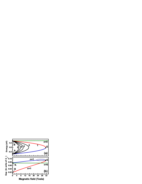
Figure 1: (a) The LLs of the effective 2D tachyonic Hamiltonian (1) are shown as a function of the magnetic field. The numbers next to the lines are the LL indices. The $n=1$ LL wave functions at points A and B are identical to conventional ‘nonrelativistic’ LLs with indices 0 and 1, respectively. At point G, the LL wave function of the tachyon system is identical to the $n=1$ LL wave function of graphene. (b) $\nu=\frac{1}{3}$-FQHE gap is shown for the $n=0$ and $n=1$ LLs of tachyons. The FQHE gap is calculated for a finite-size system with $N=9$ particles in a spherical geometry with parameter $S=12$. The red and blue lines correspond to the $n=1$ LL branches shown in panel (a). The FQHE gap is measured in units of the Coulomb energy, $\epsilon_{\rm C}=e^{2}/\kappa\ell_{0}$. The dashed curve is explained in the text.

The LL energy spectrum obtained from Eq. (3) is shown in Fig. 1. The energy spectrum for tachyons exhibits a few distinct features: (i) The LL energy spectrum is mainly restricted within the energy interval $-\Delta_{0}<E_{n,s}<\Delta_{0}$. (ii) At a given magnetic field $B$, only the LL with index $n<B^{*}/B$ can be observed. Therefore, for a given magnetic field, only a few LLs exist in the system and, for a large enough magnetic field (e.g., $B>32$ Tesla in Fig. 1(a)), only the $n=0$ LL survives. This behavior of the LL of tachyonic excitations is totally different from that in the ‘non-relativistic’ semiconductor systems with the LL energy spectrum $E_{n}\propto nB$, and “relativistic” graphene system with the LL energy spectrum $E_{n}\propto\sqrt{nB}$ abergeletal . However, there is one similarity between the tachyonic LL dispersion relations and that in graphene. In both cases there is one $n=0$ LL, the energy of which is independent of the strength of the magnetic field (without the Zeeman splitting). In graphene, the energy of this LL is $E_{n=0}=0$, while for the tachyonic excitations, $E_{n=0}=\Delta_{0}$. In both cases the corresponding wave functions are $\phi_{n=0,m}$.

To address the similarities and differences between the LL wave functions of the tachyonic system and those of graphene (or even conventional semiconductor systems), we consider the interaction properties of tachyonic excitations in a given LL. To characterize the strength of the inter-tachyonic interactions we study the strength of the FQHE, i.e., the magnitude of the FQHE gap. In the FQHE regime the electrons partially occupy a single LL and the properties of such a system are characterized by the inter-particle interactions within the corresponding LL FQHE_book . The interaction strength within a given LL is determined from the Haldane pseudopotentials, $V_{m}$ Haldane_83 , which are the interaction energies of two particles with relative angular momentum $m$. The pseudopotentials are determined from Haldane_83

$$V_{m}^{(n)}=\int_{0}^{\infty}\frac{dq}{2\pi}qV(q)\left[F_{n}(q)\right]^{2}L_{m}(q^{2})e^{-q^{2}},$$ (5)

where $L_{m}(x)$ are the Laguerre polinomials, $V(q)=2\pi e^{2}/(\kappa\ell_{0}q)$ is the Coulomb interaction in the momentum space, $\kappa$ is the dielectric constant, and $F_{n}(q)$ is the form factor for the $n$-th Landau level. The form factor is determined by the structure of the LL wave functions. For the tachyonic system the form factor is given by

$$F_{n=0}(q)=L_{0}\left({\textstyle{1\over 2}}q^{2}\right)$$ (6)

$$F_{n\geq 1}(q)=\cos^{2}\alpha_{n,s}L_{n}\left({\textstyle{1\over 2}}q^{2}\right)+\sin^{2}\alpha_{n,s}L_{n-1}\left({\textstyle{1\over 2}}q^{2}\right).$$ (7)

The form factor of the $n=0$ LL [Eq. (6)] is identical to that of graphene and also to that of the non-relativistic systems. However, for $n\geq 1$ the form factor of the tachyonic system becomes unique. For graphene and for the non-relativistic systems the corresponding form factors are $F_{n}^{\rm(NR)}=L_{n}$ and $F_{n}^{\rm(Gr)}=\frac{1}{2}(L_{n}+L_{n-1})$, respectively. In both cases the form factors are independent of the magnetic field. For the tachyonic system, on the other hand, the form factor (7) depends on the magnetic field, through the effective angle $\alpha_{n,s}(B)$. With increasing magnetic field the tachyonic form factor, $F_{n\geq 1}$, changes from the non-relativistic value, $F_{n}^{(NR)}$ [point B in Fig. 1(a)] or $F_{n-1}^{(NR)}$ [point A in Fig. 1(a)], in a small magnetic field, $B\rightarrow 0$, to the form factor of graphene, $F_{n}^{\rm(Gr)}=\frac{1}{2}(L_{n}+L_{n-1})$ Apalkov_06 , for $B=B^{*}$.

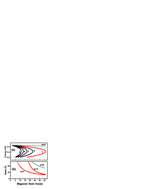
Figure 2: (a) The LL energy spectrum of a electron in a junction between two TIs is shown as a function of magnetic field for a few lowest LLs. The numbers next to the lines are the LL indexes. The TIs have the same Hamiltonian parameters, except $A_{1}$, which takes the values: $A_{1}=2.2$ eV$\cdot$Å for TI-1 and $A_{1}=4.0$ eV$\cdot$Å for TI-2. (b) The width in the $z$-direction of the LL wave functions is shown for $n=0$ and $n=1$ LLs. The corresponding LL energy spectrum is shown in panel (a).

The FQHE with an incompressible ground state can be observed only in the LL with strong short-range repulsion, i.e., a fast decay of the corresponding pseudopotentials, $V_{m}$, with $m$. Such a strong repulsion is realized only in the LL with a strong admixture of $\phi_{0,m}$. Therefore, in a tachyonic system the FQHE is expected only in the $n=0$ and $n=1$ LLs. To study the strength of the corresponding FQHE we numerically evaluate the energy spectrum of a finite $N$-electron system in a spherical geometry Haldane_83 with the radius of the sphere $\sqrt{S}\ell_{0}$. Here $2S$ is the integer number of magnetic fluxes through the sphere in units of the flux quantum. For a given number of electrons, the radius of the sphere determines the filling factor of the system. For example, the $\nu=1/q$ FQHE ($q$ is an odd integer) corresponds to the relation $S=(\frac{q}{2})(N-1)$ FQHE_book .

In Fig. 1(b) the $\nu=\frac{1}{3}$-FQHE gap is shown for $n=0$ and $n=1$ LLs of the tachyonis system. For the $n=0$ LL, the FQHE gap does not depend on $B$ and the gap exactly equals to the FQHE gap for the $n=0$ non-relativistic LL. This is because the $n=0$ tachyonic LL wave function consists of only the functions $\phi_{0,m}$. For the $n=1$ LL, the wave function is the $B$-dependent mixture of $\phi_{0,m}$ and $\phi_{1,m}$. As a result the FQHE gap depends on the magnetic field and changes from the $n=0$ non-relativistic LL value for $B\rightarrow 0$ (point A) to the $n=1$ graphene LL value for $B=B^{*}$ (point G) and finally to $n=1$ non-relativistic LL value at point B (in the thermodynamic limit such a state becomes compressible).

The maximum FQHE gap in a non-relativistic system corresponds to the green line in Fig. 1(b), while the maximum FQHE gap in the graphene system corresponds to point G in Fig. 1(b). Therefore, comparing the data in Fig. 1(b), we conclude that within some range of the magnetic fields (which is shown in Fig. 1(b) by an oval curve), the FQHE gap in the model tachyonic system is the largest compared to other available 2D systems. The tachyonic dispersion relation provides an unique possibility to study, within a single tachyonic $n=1$ LL, the properties of the $n=0$ non-relativistic LL [point A in Fig. 1(a)], $n=1$ graphene LL [point G in Fig. 1(a)], and $n=1$ non-relativistic LL [point B in Fig. 1(a)].

Three-dimensional (3D) model for the junction states between two TIs: Until now, we have discussed the magnetic field effects via an effective Hamiltonian for tachyons. The tachyonic dispersion can be realized in the junction of two TIs tachyon . The junction dispersion relation in this case is approximately described by the effective Hamiltonian (1). The realization of the tachyonic excitations as the junction states bring additional factors into consideration. For example, the junction states have a finite width in the $z$-direction which can reduce the interaction strength in that system.

We consider the junction between two TI insulators: TI-1 for $z<0$ and TI-2 for $z>0$. Here $z=0$ corresponds to the junction surface. The electronic properties of both TIs are described by the same type of low-energy effective 3D Hamiltonian liu_2010 ; zhang_2009 of the matrix form

$${\cal H}_{\rm TI}=\epsilon(\vec{k})+\left(\begin{array}[]{cc}M(\vec{p})\sigma_{z}-{\rm i}A_{1}\sigma_{x}\partial_{z}&(A_{2}/\hbar)p_{-}\sigma_{x}\\ (A_{2}/\hbar)p_{+}\sigma_{x}&M(\vec{p})\sigma_{z}+{\rm i}A_{1}\sigma_{x}\partial_{z}\end{array}\right),$$ (8)

where $\partial_{z}=\partial/\partial z$, and

$$\epsilon(\vec{k})=C_{1}-D_{1}\partial_{z}^{2}+(D_{2}/\hbar^{2})(p_{x}^{2}+p_{y}^{2}),$$ (9)

$$M(\vec{k})=M_{0}+B_{1}\partial_{z}^{2}-(B_{2}/\hbar^{2})(p_{x}^{2}+p_{y}^{2}).$$ (10)

We assume that for TI-1 the constants in the above Hamiltonian are the same as for $\mbox{Bi}_{2}\mbox{Se}_{3}$ zhang_2009 , while the for TI-2 the constants are different but close to the values for $\mbox{Bi}_{2}\mbox{Se}_{3}$. We assume that only the constant $A_{1}$ is different for the two TIs, i.e., $A_{1}=2.2$ eV$\cdot$Å for TI-1 and $A_{1}=4.0$ eV$\cdot$Å for TI-2. All other constants in the Hamiltonian (8) are kept the same for both TIs tachyon . For these parameters, the junction states exhibit the tachyonic dispersion tachyon . The four-component wave function corresponding to the Hamiltonian (8) determines the amplitudes of the wave functions at the positions of Bi and Se atoms: $(\mbox{Bi}_{\uparrow},\mbox{Se}_{\uparrow},\mbox{Bi}_{\downarrow},\mbox{Se}_{\downarrow})$, where the arrows indicate the direction of the electron spin.

The Hamiltonian of the TI in an external magnetic field, pointing along the $z$-direction, can be obtained from the Hamiltonian (8) by replacing the 2D momentum $(p_{x},p_{y})$ by the generalized momentum $(\pi_{x},\pi_{y})$ yang_2011 and introducing the Zeeman energy, $\Delta_{z}=\frac{1}{2}g_{s}\mu_{B}B$. For the Hamiltonian (8) in a magnetic field, the wave function in the $n$-th LL has the general form

$$\Psi^{\rm(TI)}_{n\geq 1}(z)=\left(\begin{array}[]{c}\chi^{(n)}_{1}(z)\phi_{n-1,m}\\ \chi^{(n)}_{2}(z)\phi_{n-1,m}\\ \chi^{(n)}_{3}(z)\phi_{n,m}\\ \chi^{(n)}_{4}(z)\phi_{n,m}\end{array}\right).$$ (11)

Therefore, just as for the tachyonic states the wave function $\Psi^{\rm(TI)}_{n\geq 1}$ is the mixture of $n$ and $n-1$ non-relativistic LL functions. For the $n=0$ LL, only $\chi^{(n=0)}_{3}$ and $\chi^{(n=0)}_{4}$ are non-zero.

To find the LL junction states we follow the same procedure as for the LL surface states of a TI zhou_2008 ; shan_2010 ; yang_2011 . For each TI we find the general bulk solution of the Schrödinger equation in the form of $\Psi\propto e^{\lambda^{(m)}z}$, where $\lambda^{(m)}$ is a complex constant, and $m=1$ and 2 for TI-1 and TI-2, respectively. This solution has a given energy, $E$, and a given LL index, $n$. The corresponding $\lambda^{(m)}$ are determined from a secular equation, $\det\left[{\cal{H}}^{(m)}_{TI}(\vec{k},\lambda^{(m)})-E\right]=0$, for each TI. For each energy $E$ and the LL index $n$, the secular equation provides eight values of $\lambda^{(m)}_{j}(n,E)$, $j=1,\ldots,8$ with the corresponding wave functions. Second, since we are looking for the localized LL junction states, we need to choose (for each TI) only four values of $\lambda^{(m)}_{j}$ out of eight with the properties: $\mbox{Re}\lambda^{(m)}_{j}>0$ for TI-1 ($z<0$) and $\mbox{Re}\lambda^{(m)}_{j}<0$ for TI-2 ($z>0$). We then choose the corresponding four wave functions (for each TI) as the basis and expand the solution for the LL junction state in this basis. Finally, the energy of the LL junction state is found from the condition of continuity of the wave function, $\Psi^{\rm(TI)}_{n}(z)$, and current $[\delta{\cal H}_{\rm TI}/\delta k_{z}]\Psi^{\rm(TI)}_{n}$ in the junction.

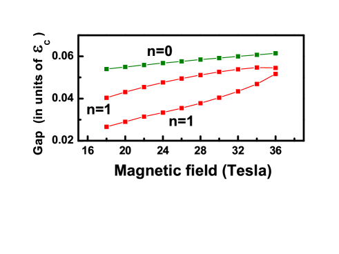
Figure 3: The $\nu=\frac{1}{3}$ FQHE gap for $n=0$ (green line) and $n=1$ (red line) LLs in the junction of two TIs. The corresponding LLs are shown in Fig. 2(a) by green and red lines, respectively. The FQHE gap is calculated for a finite-size system with $N=9$ particles in spherical geometry with parameter $S=12$. The FQHE gap is measured in units of Coulomb energy, $\epsilon_{\rm C}=e^{2}/\kappa\ell_{0}$.

The spectrum of the LL junction states corresponding to the tachyonic dispersion is shown in Fig. 2(a). The spectrum is qualitatively similar to that [see Fig. 1(a)] obtained from the model 2D Hamiltonian. Both spectra have the finite range of magnetic fields and energies, where the LLs can be observed. At weak magnetic fields, the difference between the LL spectrum of the junction states and the 2D model is clearly visible. For a given LL index $n$, there are no junction states for weak magnetic fields. These junction states are delocalized in the $z$-direction. To illustrate this delocalization we show in Fig. 2(b) the width of the $n=0$ and $n=1$ LL wave functions in the $z$-direction. At a singular point of the LL spectrum, i.e., for $B=B^{*}$, where the derivative of the LL energy with the magnetic field becomes infinitely large, the LL wave functions have the smallest width. This width increases with decreasing magnetic field and finally the LL junction states are delocalized in the $z$-direction. A similar behavior is observed for $n=0$ LL, but there are no singular point in this case. Therefore, the LL energy spectrum of the junction states in the regime of tachyonic dispersion can be well described within 2D effective model near the singular point $B\sim B^{*}$.

We have evaluated the FQHE gaps for the $n=0$ and $n=1$ junction LLs. We have used the same approach as for the 2D model of the tachyonic excitations, discussed above. The results are shown in Fig. 3. Quantitatively the behavior of the FQHE gap as a function of the magnetic field is similar to the 2D model of the tachyonic excitations [Fig. 1(b)]. Due to a finite width of the LL wave functions in the TI junction, there is a reduction of the inter-electron interaction strength and correspondingly the FQHE gap. This reduction is visible for $n=0$ LL, where a smaller FQHE gap and the magnetic field dependence of the FQHE gap is shown in Fig. 3.

Although for the 2D tachyonic model the FQHE gap is the largest for the $n=1$ LL, for the junction LLs the FQHE gap is the largest for the $n=0$ LL, due to the non-zero spin polarization of the $n=1$ junction LL. This spin polarization is clearly visible from the general property of the LL wave function [Eq. (11)]; only the components $\chi_{3}^{(n=0)}$ and $\chi_{4}^{(n=0)}$ of $\Psi_{n=0}^{\rm(TI)}$ are non-zero and these components correspond to the spin-down polarization. The numerically found $n=1$ LL wave functions also show partial spin-down polarization. As a result, the LL wave function have larger contribution from the $\phi_{n=1}$ non-relativistic LL function, which reduces the inter-electron interaction strength and the FQHE gap.

To summarize: we have investigated the magnetic field effects of tachyonic excitations along the interface of two topological insulators. We used an effective two-dimensional model Hamiltonian for tachyons and the three-dimensional model for the junction states of the two TIs, both developed by us tachyon . The Landau levels in both these models show very similar behaviors. Unlike in graphene or in conventional electron systems, only a few LLs are found to exist for the tachyons. Only one LL ($n=0$) survives for large magnetic fields. The $\nu=\frac{1}{3}$ FQHE is the strongest (within a limited range of the magnetic field) when compared with that for conventional electron systems and graphene. Interestingly, the FQHE in the $n=1$ LLs for tachyons describes the FQHE of the $n=0,1$ LLs of the non-relativistic electron system and that of the $n=1$ graphene LL in different regions of the magnetic field. Experimental confirmation of these properties of the Landau levels would provide strong evidence on the existence of elusive tachyons.

The work has been supported by the Canada Research Chairs Program of the Government of Canada.

References

- (1) Electronic address: tapash@physics.umanitoba.ca
- (2) M.Z. Hasan and C.L. Kane, Rev. Mod. Phys. 82, 3045 (2010); X.-L. Qi and S.-C. Zhang, ibid. 83, 1057 (2011).
- (3) D.S.L. Abergel, V. Apalkov, J. Berashevich, K. Ziegler, and T. Chakraborty, Adv. Phys. 59, 261 (2010).
- (4) V. Apalkov and T. Chakraborty, arXiv: 1203.5761 (2012).
- (5) O.M.P. Bilaniuk, V.K. Deshpande, and E.C.G. Sudarshan, Am. J. Phys. 30, 718 (1962); O.M. Bilaniuk, and E.C.G. Sudarshan, Phys. Today 22, No. 5, 43 (1969); G. Feinberg, Phys. Rev. 159, 1089 (1967); E. Recami, J. Phys. Conf. Ser. 196, 012020 (2009); Found. Phys. 31, 1119 (2001).
- (6) R.Y. Chiao, A.E. Kozhekin, and G. Kurizki, Phys. Rev. Lett. 77, 1254 (1996).
- (7) R. Takahashi and S. Murakami, Phys. Rev. Lett. 107, 166805 (2011).
- (8) A. Chodos, A.I. Hauser, and V.A. Kostelecky, Phys. Lett. B 150, 431 (1985); R. Ehrlich, Am. J. Phys. 71, 1109 (2003).
- (9) C.-X. Liu, X.-L. Qi, H.J. Zhang, X. Dai, Z. Fang, and S.-C. Zhang, Phys. Rev. B 82, 045122 (2010).
- (10) Z. Wang, Z.-G. Fu, S.-Xi Wang, P. Zhang, Phys. Rev. B 82, 085429 (2010.
- (11) T. Chakraborty and P. Pietiläinen, The Quantum Hall Effects (Springer, New York 1995) 2nd. edition.
- (12) F.D.M. Haldane, Phys. Rev. Lett. 51, 605 (1983).
- (13) V.M. Apalkov and T. Chakraborty, Phys. Rev. Lett. 97, 126801 (2006)
- (14) H. Zhang, C.-X. Liu, X.-L. Qi, Xi Dai, Z. Fang, and S.-C. Zhang, Nat. Phys. 5, 438 (2009).
- (15) Z. Yang and J.H. Han, Phys. Rev. B 83, 045415 (2011)
- (16) B. Zhou, H.Z. Lu, R.L. Chu, S.Q. Shen, and Q. Niu, Phys. Rev. Lett. 101 246807 (2008).
- (17) W.-Y. Shan, H.-Z. Lu, S.-Q. Shen, New J. Phys. 12 043048 (2010).