Integrability of higher pentagram maps

Abstract

We define higher pentagram maps on polygons in ${\mathbb{P}}^{d}$ for any dimension $d$, which extend R. Schwartz’s definition of the 2D pentagram map. We prove their integrability by presenting Lax representations with a spectral parameter for scale invariant maps. The corresponding continuous limit of the pentagram map in dimension $d$ is shown to be the $(2,d+1)$-equation of the KdV hierarchy, generalizing the Boussinesq equation in 2D. We also study in detail the 3D case, where we prove integrability for both closed and twisted polygons and describe the spectral curve, first integrals, the corresponding tori and the motion along them, as well as an invariant symplectic structure.

1 Introduction

The pentagram map was defined by R. Schwartz in [13] on plane convex polygons considered modulo projective equivalence. Figure 1 explains the definition: for a polygon $P$ the image under the pentagram map is a new polygon $T(P)$ spanned by the “shortest” diagonals of $P$. Iterations of this map on classes of projectively equivalent polygons manifest quasiperiodic behaviour, which indicates hidden integrability [14].

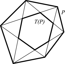
Figure 1: The image $T(P)$ of a hexagon $P$ under the 2D pentagram map.

The integrability was proved in [11] for the pentagram map on a larger class of the so called twisted polygons in 2D, which are piecewise linear curves with a fixed monodromy relating their ends. Closed polygons correspond to the monodromy given by the identity transformation. It turned out that there is an invariant Poisson structure for the pentagram map and it has sufficiently many invariant quantities. Moreover, this map turned out to be related to a variety of mathematical domains, including cluster algebras [2, 4], frieze patterns, and integrable systems of mathematical physics: in particular, its continuous limit in 2D is the classical Boussinesq equation [11]. Integrability of the pentagram map for 2D closed polygons was established in [15, 12], while a more general framework related to surface networks was presented in [3].

In this paper we extend the definition of the pentagram map to closed and twisted polygons in spaces of any dimension $d$ and prove its various integrability properties. It is worth mentioning that the problem of finding integrable higher-dimensional generalizations for the pentagram map attracted much attention after the 2D case was treated in [11]. The main difficulty in higher dimensions is that diagonals of a polygon are generically skew and do not intersect. One can either confine oneself to special polygons (e.g., corrugated ones, [3]) to retain the intersection property or one has too many possible choices for using hyperplanes as diagonals, where it is difficult to find integrable ones, cf. [9].

Below, as an analog of the 2D shortest diagonals for a generic polygon in a projective space ${\mathbb{RP}}^{d}$ we propose to consider a “short-diagonal hyperplane” passing through $d$ vertices where every other vertex is taken starting with a given one. Then a new vertex is constructed as the intersection of $d$ consecutive diagonal hyperplanes. We repeat this procedure starting with the next vertex of the initial polygon. The higher (or $d$-dimensional) pentagram map $T$ takes the initial polygon to the one defined by this set of new vertices. As before, the obtained polygon is considered modulo projective equivalence in ${\mathbb{RP}}^{d}$.

We also describe general pentagram maps $T_{p,r}$ in ${\mathbb{RP}}^{d}$ enumerated by two integral parameters $p$ and $r$ by considering $p$-diagonals (i.e., hyperplanes passing through every $p$th vertex of the polygon) and by taking the intersections of every $r$th hyperplane like that. There is a curious duality between them: the map $T_{p,r}$ is equal to $T^{-1}_{r,p}$ modulo a shift in vertex indices. However, we are mostly interested in the higher pentagram maps, which correspond to $T:=T_{2,1}$ in ${\mathbb{RP}}^{d}$.

We start by describing the continuous limit of the higher pentagram map as the evolution in the direction of the “envelope” for such a sequence of short-diagonal planes as the number of vertices of the polygon tends to infinity. (More precisely, the envelope here is the curve whose osculating planes are limits of the short-diagonal planes.)

Theorem A.

(= Theorems 4.3, 4.5) The continuous limit of the higher pentagram map in ${\mathbb{RP}}^{d}$ is the $(2,d+1)$-equation in the KdV hierarchy, which is an infinite-dimensional completely integrable system.

This generalizes the Boussinesq equation as a limit of the pentagram map in ${\mathbb{RP}}^{2}$ and this limit seems to be very robust. Indeed, the same equation appears for an almost arbitrary choice of diagonal planes. It also arises when instead of osculating planes one considers other possible definitions of higher pentagram maps (cf. e.g. [9]).

However, the pentagram map in the above definition with short-diagonal hyperplanes exhibits integrability properties not only in the continuous limit, but as a discrete system as well. To study them, we define two coordinate systems for twisted polygons in 3D (somewhat similar to the ones used in 2D, cf. [11]), and present explicit formulas for the 3D pentagram map using these coordinates (see Theorem 5.6).

Then we describe the pentagram map as a completely integrable discrete dynamical system by presenting its Lax form in any dimension and studying in detail the 3D case (see Section 6). For algebraic-geometric integrability we complexify the pentagram map. The corresponding 2D case was investigated in [15].

The key ingredient of the algebraic-geometric integrability for a discrete dynamical system is a discrete Lax (or zero curvature) equation with a spectral parameter, which in our case assumes the following form:

$$L_{i,t+1}(\lambda)=P_{i+1,t}(\lambda)L_{i,t}(\lambda)P_{i,t}^{-1}(\lambda).$$

Here the index $t$ represents the discrete time variable, the index $i$ refers to the vertex of an $n$-gon, and $\lambda$ is a complex spectral parameter. (For the pentagram map in ${\mathbb{CP}}^{d}$ the functions $L_{i,t}(\lambda)$ and $P_{i,t}(\lambda)$ are matrix-valued of size $(d+1)\times(d+1)$.) The discrete Lax equation arises as a compatibility condition of an over-determined system of equations:

$$\begin{cases}L_{i,t}(\lambda)\Psi_{i,t}(\lambda)=\Psi_{i+1,t}(\lambda)\\ P_{i,t}(\lambda)\Psi_{i,t}(\lambda)=\Psi_{i,t+1}(\lambda),\end{cases}$$

for an auxiliary function $\Psi_{i,t}(\lambda)$.

Remark 1.1.

Recall that for a smooth dynamical system the Lax form is a differential equation of type $\partial_{t}L=[P,L]$ on a matrix $L$. Such a form of the equation implies that the evolution of $L$ changes it to a similar matrix, thus preserving its eigenvalues. If the matrix $L$ depends on a parameter, $L=L(\lambda)$, then the corresponding eigenvalues as functions of parameter do not change and in many cases provide sufficiently many first integrals for complete integrability of such a system.

Similarly, an analogue of the Lax form for differential operators of type $\partial_{x}-L$ is a zero curvature equation $\partial_{t}L-\partial_{x}P=[P,L]\,.$ This is a compatibility condition which provides the existence of an auxiliary function $\psi=\psi(t,x)$ satisfying a system of equations $\partial_{x}\psi=L\psi$ and $\partial_{t}\psi=P\psi\,.$ The above Lax form and auxiliary system are discrete versions of the latter.

In our case, the equivalence of formulas for the pentagram map to the dynamics defined by the Lax equation implies complete algebraic-geometric integrability of the system. More precisely, the following theorem summarizes several main results on the 3D pentagram map, which are obtained by studying its Lax equation. The dynamics is (generically) defined on the space ${\mathcal{P}}_{n}$ of projectively equivalent twisted $n$-gons in 3D, which we describe below, and has dimension $3n$, while closed $n$-gons form a submanifold of codimension 15 in it.

Later on we will introduce the notion of spectral data which consists of a Riemann surface, called a spectral curve, and a point in the Jacobian (i.e., the complex torus) of this curve, as well as a notion of a spectral map between the space ${\mathcal{P}}_{n}$ and the spectral data.

Theorem B.

(= Theorems 6.15, 6.19, 7.1) A Zariski open subset of the complexified space ${\mathcal{P}}_{n}$ of twisted $n$-gons in 3D is a fibration whose fibres are Zariski open subsets of tori. These tori are Jacobians of the corresponding spectral curves and are invariant with respect to the space pentagram map. Their dimension is $3\lfloor n/2\rfloor$ for odd $n$ and $3(n/2)-3$ for even $n$, where $\lfloor n/2\rfloor$ is the integer part of $n/2$.

The pentagram dynamics on the Jacobians goes along a straight line for odd $n$ and along a staircase for even $n$ (i.e., the discrete evolution is either a constant shift on a torus, or its square is a constant shift).

For closed $n$-gons the tori have dimensions $3\lfloor n/2\rfloor-6$ for odd $n$ and $3(n/2)-9$ for even $n$.

Remark 1.2.

One also has an explicit description of the the above fibration in terms of coordinates on the space of $n$-gons. We note that the pentagram dynamics understood as a shift on complex tori does not prevent the corresponding orbits on the space ${\mathcal{P}}_{n}$ from being unbounded. The dynamics described above takes place for generic initial data, i.e., for points on the Jacobians whose orbits do not intersect certain divisors. Points of generic orbits with irrational shifts can return arbitrarily close to such divisors. On the other hand, the inverse spectral map is defined outside of these special divisors and may have poles there. Therefore the sequences in the space ${\mathcal{P}}_{n}$ corresponding to such orbits may escape to infinity.

It is known that the pentagram map in 2D possesses an invariant Poisson structure [11], which can also be described by using the Krichever-Phong universal formula [15]. Although we do not present an invariant Poisson structure for the pentagram map in 3D, we describe its symplectic leaves, as well as the action-angle coordinates. More precisely, we present an invariant symplectic structure (i.e., a closed non-degenerate 2-form), and submanifolds where it is defined (Theorem 7.5). By analogy with the 2D case, it is natural to suggest that these submanifolds are symplectic leaves of an invariant Poisson structure, and that the inverse of our symplectic structure coincides with the Poisson structure on the leaves. An explicit description of this Poisson structure in 3D is still an open problem.

Note that the algebraic-geometric integrability of the pentagram map implies its Arnold–Liouville complete integrability on generic symplectic leaves (in the real case). Namely, the existence of a (pre)symplectic structure coming from the Lax form of the pentagram map (see Section 7.2), together with the generic set of first integrals, appearing as coefficients of the corresponding spectral curve, provides sufficiently many integrals in involution. (Note that proving independence of first integrals while remaining within the real setting is often more difficult than first proving the algebraic-geometric integrability, which in turn implies their independence in the real case.)

Finally, in Section 8 we present a Lax form for the pentagram maps in arbitrary dimension (which implies their complete integrability) assuming their scaling invariance:

Theorem C.

(= Theorem 8.3) The scale-invariant pentagram map in ${\mathbb{CP}}^{d}$ admits a Lax representation with a spectral parameter.

The scaling invariance of the pentagram maps is proved for all $d\leq 6$, with some numerical evidence for higher values of $d>6$ as well. It would be interesting to establish it in full generality. There is a considerable difference between the cases of even and odd dimension $d$, which can be already seen in the analysis of the 2D and 3D cases.

Acknowledgments. We are grateful to M. Gekhtman and S. Tabachnikov for useful discussions. B.K. was partially supported by the Simonyi Fund and an NSERC research grant.

2 Review of the 2D pentagram map

In this section we recall the main definitions and results in 2D (see [11]), which will be important for higher-dimensional generalizations below. We formulate the geometric results in the real setting, while the algebraic-geometric ones are presented for the corresponding complexification.

First note that the pentagram map can be extended from closed to twisted polygons.

Definition 2.1.

Given a projective transformation $M\in PSL(3,{\mathbb{R}})$ of the plane ${\mathbb{RP}}^{2}$, a twisted $n$-gon in ${\mathbb{RP}}^{2}$ is a map $\phi:{\mathbb{Z}}\to{\mathbb{RP}}^{2}$, such that $\phi(k+n)=M\circ\phi(k)$ for any $k$. $M$ is called the monodromy of $\phi$. Two twisted $n$-gons are equivalent if there is a transformation $g\in PSL(3,{\mathbb{R}})$ such that $g\circ\phi_{1}=\phi_{2}$.

Consider generic $n$-gons, i.e., those that do not have any three consecutive vertices lying on the same line. Denote by ${\mathcal{P}}_{n}$ the space of generic twisted $n$-gons considered up to $PSL(3,{\mathbb{R}})$ transformations. The dimension of ${\mathcal{P}}_{n}$ is $2n$. Indeed, a twisted $n$-gon depends on $2n$ variables representing coordinates of vertices $v_{k}:=\phi(k)$ for $k=1,...,n$ and on 8 parameters of the monodromy matrix $M$, while the $PSL(3,{\mathbb{R}})$-equivalence reduces the dimension by 8. The pentagram map $T$ is generically defined on the space ${\mathcal{P}}_{n}$. Namely, for a twisted $n$-gon vertices of its image are the intersections of pairs of consecutive shortest diagonals: $Tv_{k}:=(v_{k-1},v_{k+1})\cap(v_{k},v_{k+2})$. Such intersections are well defined for a generic point in ${\mathcal{P}}_{n}$.

a) Results on integrability (in the twisted and closed cases). There is a Poisson structure on ${\mathcal{P}}_{n}$ invariant with respect to the pentagram map. There are $2\lfloor n/2\rfloor+2$ integrals in involution, which provide integrability of the pentagram map on ${\mathcal{P}}_{n}$. Its symplectic leaves have codimensions 2 or 4 in ${\mathcal{P}}_{n}$ depending on whether $n$ is odd or even, and the invariant tori have dimensions $n-1$ or $n-2$, respectively [11].

Moreover, when restricted to the space ${\mathcal{C}}_{n}$ of closed polygons ($\dim{\mathcal{C}}_{n}=2n-8=2(n-4)$), the map is still integrable and has invariant tori of dimension $n-4$ for odd $n$ and $n-5$ for even $n$. Note that the space ${\mathcal{C}}_{n}$ of closed polygons is not a Poisson submanifold in the space ${\mathcal{P}}_{n}$ of twisted $n$-gons, so the corresponding Poisson structure on ${\mathcal{P}}_{n}$ cannot be restricted to ${\mathcal{C}}_{n}$.

There is a Lax representation for the pentagram map. Coefficients of the corresponding spectral curve are the first integrals of the dynamics. The pentagram map defines a discrete motion on the Jacobian of the spectral curve. This motion is linear or staircase-like depending on the parity of $n$, see [15].

b) Coordinates on ${\mathcal{P}}_{n}$. The following two systems of coordinates on ${\mathcal{P}}_{n}$ are particularly convenient to work with, see [11]. Assume that $n$ is not divisible by 3. Then there exists a unique lift of points $v_{k}=\phi(k)\in{\mathbb{RP}}^{2}$ to the vectors $V_{k}\in{\mathbb{R}}^{3}$ satisfying the condition $\det|V_{j},V_{j+1},V_{j+2}|=1$ for each $j$. Associate a difference equation to a sequence of vectors $V_{k}\in{\mathbb{R}}^{3}$ by setting

$$V_{j+3}=a_{j}V_{j+2}+b_{j}V_{j+1}+V_{j}$$

for all $j\in{\mathbb{Z}}$. The sequences $(a_{j})$ and $(b_{j})$ turn out to be $n$-periodic, which is a manifestation of the fact that the lifts satisfy the relations $V_{j+n}=MV_{j},\;j\in{\mathbb{Z}},$ for a certain monodromy matrix $M\in SL(3,{\mathbb{R}})$. The variables $a_{j},b_{j},\,0\leq j\leq n-1$ are coordinates on the space ${\mathcal{P}}_{n}$.

There exists another coordinate system on the space ${\mathcal{P}}_{n}$, which is more geometric. Recall that the cross-ratio of 4 points in ${\mathbb{P}}^{1}$ is given by

$$[t_{1},t_{2},t_{3},t_{4}]=\frac{(t_{1}-t_{2})(t_{3}-t_{4})}{(t_{1}-t_{3})(t_{2}-t_{4})},$$

where $t$ is any affine parameter. Now associate to each vertex $v_{i}$ the following two numbers, which are the cross-ratios of two 4-tuples of points lying on the lines $(v_{i-2},v_{i-1})$ and $(v_{i+1},v_{i+2})$ respectively:

$$x_{i}=[v_{i-2},\,v_{i-1},\,((v_{i-2},v_{i-1})\cap(v_{i},v_{i+1})),\,((v_{i-2},v_{i-1})\cap(v_{i+2},v_{i+2}))]$$

$$y_{i}=[((v_{i-2},v_{i-1})\cap(v_{i+1},v_{i+2})),((v_{i-1},v_{i})\cap(v_{i+1},v_{i+2})),\,v_{i+1},\,v_{i+2}]$$

In these coordinates the pentagram map has the form

$$T^{*}x_{i}=x_{i}\frac{1-x_{i-1}y_{i-1}}{1-x_{i+1}y_{i+1}}\,\qquad T^{*}y_{i}=y_{i+1}\frac{1-x_{i+2}y_{i+2}}{1-x_{i}y_{i}}\,.$$

One can see that the pentagram map commutes with the scaling transformation [11, 14]:

$$R_{s}:\,(x_{1},y_{1},...,x_{n},y_{n})\to(sx_{1},s^{-1}y_{1},...,sx_{n},s^{-1}y_{n})\,.$$

In these coordinates the invariant Poisson structure has a particularly simple form, see [11].

c) Continuous limit: the Boussinesq equation. The $n\to\infty$ continuous limit of a twisted $n$-gon with a fixed monodromy $M\in PSL(3,{\mathbb{R}})$ can be viewed as a smooth parameterized curve $\gamma:{\mathbb{R}}\to{\mathbb{RP}}^{2}$ satisfying $\gamma(x+2\pi)=M\gamma(x)$ for all $x\in{\mathbb{R}}$. The genericity assumption that every three consecutive points of an $n$-gon are in general position corresponds to the assumption that $\gamma$ is a non-degenerate curve in ${\mathbb{RP}}^{2}$, i.e., the vectors $\gamma^{\prime}(x)$ and $\gamma^{\prime\prime}(x)$ are linearly independent for all $x\in{\mathbb{R}}$.

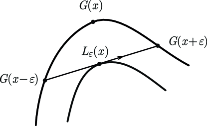
Figure 2: Constructing the envelope $L_{\epsilon}(x)$ in 2D.

The space of such projectively equivalent curves is in one-to-one correspondence with linear differential operators of the third order: $L=\partial^{3}+u_{1}(x)\partial+u_{0}(x)$, where the coefficients $u_{0}$ and $u_{1}$ are periodic in $x$. Namely, a curve $\gamma(x)$ in ${\mathbb{RP}}^{2}$ can be lifted to a quasi-periodic curve $G=\{G(x)\}$ in ${\mathbb{R}}^{3}$ satisfying $\det|G(x),G^{\prime}(x),G^{\prime\prime}(x)|=1$ for all $x\in{\mathbb{R}}$. The components of the vector function $G(x)=(G_{1}(x),G_{2}(x),G_{3}(x))$ are homogenous coordinates of $\gamma(x)$ in ${\mathbb{RP}}^{2}$: $\gamma(x)=(G_{1}:G_{2}:G_{3})(x)\in{\mathbb{RP}}^{2}$. The vector function $G(x)$ can be identified with a solution of the unique linear differential operator $L$, i.e., the components of $G(x)$ are identified with three linearly independent solutions of the differential equation $Ly=0$.

A continuous analog of the pentagram map is obtained by the following construction. Given a non-degenerate curve $\gamma(x)$, we draw the chord $(\gamma(x-\epsilon),\gamma(x+\epsilon))$ at each point $x$. Consider the envelope $\ell_{\epsilon}(x)$ of these chords. (Figure 2 shows their lifts: chords $(G(x-\epsilon),G(x+\epsilon))$ and their envelope $L_{\epsilon}(x)$.) Let $u_{1,\epsilon}$ and $u_{0,\epsilon}$ be the periodic coefficients of the corresponding differential operator. Their expansions in $\epsilon$ have the form $u_{i,\epsilon}=u_{i}+\epsilon^{2}w_{i}+{\mathcal{O}}(\epsilon^{3})$ and allow one to define the evolution $du_{i}/dt:=w_{i}$, $i=0,1$. After getting rid of $u_{0}$ this becomes the classical Boussinesq equation on the periodic function $u=u_{1}$, which is the $(2,3)$-flow in the KdV hierarchy of integrable equations on the circle: $u_{tt}+2(u^{2})_{xx}+u_{xxxx}=0$.

Below we generalize these results to higher dimensions.

3 Geometric definition of higher pentagram maps

3.1 Pentagram map in 3D

First we extend the notion of a closed polygon to a twisted one, similar to the 2D case. We present the 3D case first, before giving the definition of the pentagram map in arbitrary dimension, since it is used in many formulas below.

Definition 3.1.

A twisted $n$-gon in ${\mathbb{RP}}^{3}$ with a monodromy ${M}\in SL(4,{\mathbb{R}})$ is a map $\phi:{\mathbb{Z}}\to{\mathbb{RP}}^{3}$, such that $\phi(k+n)=M\circ\phi(k)$ for each $k\in{\mathbb{Z}}$. (Here we consider the natural action of $SL(4,{\mathbb{R}})$ on the corresponding projective space ${\mathbb{RP}}^{3}$.) Two twisted $n$-gons are (projectively) equivalent if there is a transformation $g\in SL(4,{\mathbb{R}})$, such that $g\circ\phi_{1}=\phi_{2}$.

Note that equivalent $n$-gons must have similar monodromies. Closed $n$-gons (space polygons) correspond to the monodromies $M=\mathrm{Id}$ and $-\mathrm{Id}$. Let us assume that vertices of an $n$-gon are in general position, i.e., no four consecutive vertices belong to one and the same plane in ${\mathbb{RP}}^{3}$. Also, assume that $n$ is odd. Then one can show (see Section 5.3 below and cf. Proposition 4.1 in [11]) that there exists a unique lift of the vertices $v_{k}:=\phi(k)\in{\mathbb{RP}}^{3}$ to the vectors $V_{k}\in{\mathbb{R}}^{4}$ satisfying for all $j\in{\mathbb{Z}}$ the identities $\det|V_{j},V_{j+1},V_{j+2},V_{j+3}|=1$ and $V_{j+n}=MV_{j}$, where $M\in SL(4,{\mathbb{R}})$. These vectors satisfy difference equations

$$V_{j+4}=a_{j}V_{j+3}+b_{j}V_{j+2}+c_{j}V_{j+1}-V_{j},\;j\in{\mathbb{Z}},$$

with $n$-periodic coefficients $(a_{j},b_{j},c_{j})$ and we employ this equation to introduce the $(a,b,c)$-coordinates on the space of twisted $n$-gons.

Define the pentagram map on the classes of equivalent $n$-gons in such a way.

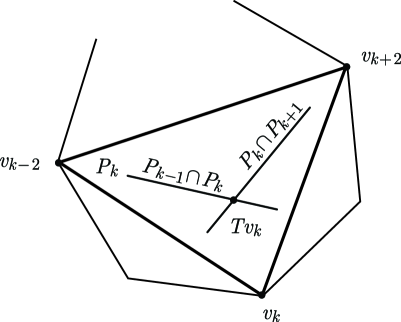
Figure 3: In 3D the image $Tv_{k}$ of the vertex $v_{k}$ is the intersection of three “short-diagonal” planes $P_{k-1},P_{k},$ and $P_{k+1}$.

Definition 3.2.

Given an $n$-gon $\phi$ in ${\mathbb{RP}}^{3}$, for each $k\in{\mathbb{Z}}$ consider the two-dimensional “short-diagonal plane” $P_{k}:=(v_{k-2},v_{k},v_{k+2})$ passing through 3 vertices $v_{k-2},v_{k},v_{k+2}$. Take the intersection point of the three consecutive planes $P_{k-1},P_{k},P_{k+1}$ and call it the image of the vertex $v_{k}$ under the space pentagram map $T$, see Figure 3. (We assume the general position, so that every three consecutive planes $P_{k}$ for the given $n$-gon intersect at a point.)

By lifting a two-dimensional plane $P_{k}$ from ${\mathbb{RP}}^{3}$ to the three-dimensional plane through the origin in ${\mathbb{R}}^{4}$ (and slightly abusing notation) we have $P_{k}=*(V_{k-2}\wedge V_{k}\wedge V_{k+2})$ in terms of the natural duality $*$ between ${\mathbb{R}}^{4}$ and ${\mathbb{R}}^{4*}$. The lift of $Tv_{k}$ to ${\mathbb{R}}^{4}$ is proportional to $*[P_{k-1}\wedge P_{k}\wedge P_{k+1}]$.

Below we describe the properties of this space pentagram map in detail.

3.2 Pentagram map in any dimension

Before defining the pentagram map in ${\mathbb{RP}}^{d}$, recall that $SL(d+1,{\mathbb{R}})$ is a two-fold cover of $PSL(d+1,{\mathbb{R}})$ for odd $d$ and coincides with the latter for even $d$.

Definition 3.3.

A twisted $n$-gon in ${\mathbb{RP}}^{d}$ with a monodromy $M\in SL(d+1,{\mathbb{R}})$ is a map $\phi:{\mathbb{Z}}\to{\mathbb{RP}}^{d}$, such that $\phi(k+n)=M\circ\phi(k)$ for each $k\in{\mathbb{Z}}$, and where $M$ acts naturally on ${\mathbb{RP}}^{d}$.

We define the $SL(d+1,{\mathbb{R}})$-equivalence of $n$-gons as above, and assume the vertices $v_{k}:=\phi(k)$ to be in general position, i.e., in particular, no $d+1$ consecutive vertices of an $n$-gon belong to one and the same $(d-1)$-dimensional plane in ${\mathbb{RP}}^{d}$.

Remark 3.4.

One can show that there exists a unique lift of the vertices $v_{k}=\phi(k)\in{\mathbb{RP}}^{d}$ to the vectors $V_{k}\in{\mathbb{R}}^{d+1}$ satisfying $\det|V_{j},V_{j+1},...,V_{j+d}|=1$ and $V_{j+n}=MV_{j},\;j\in{\mathbb{Z}},$ where $M\in SL(d+1,{\mathbb{R}})$, if and only if the condition $gcd(n,d+1)=1$ holds. The corresponding difference equations have the form

$$V_{j+d+1}=a_{j,d}V_{j+d}+a_{j,d-1}V_{j+d-1}+...+a_{j,1}V_{j+1}+(-1)^{d}V_{j},\quad j\in{\mathbb{Z}},$$ (1)

with $n$-periodic coefficients in the index $j$. This allows one to introduce coordinates $\{a_{j,k},\;0\leq j\leq n-1,\;1\leq k\leq d\}$ on the space of twisted $n$-gons in ${\mathbb{RP}}^{d}$.

For a generic twisted $n$-gon in ${\mathbb{RP}}^{d}$ one can define the “short-diagonal” $(d-1)$-dimensional plane $P_{k}$ passing through $d$ vertices of the $n$-gon by taking every other vertex starting at the point $v_{k}$, i.e., through the vertices $v_{k},v_{k+2},...,v_{k+2d-2}$. For calculations, however, it is convenient to have the set of vertices “centered” at $v_{k}$, and then the definition becomes slightly different in the odd and even dimensional cases.

Namely, for odd dimension $d=2\varkappa+1$ we consider the short-diagonal hyperplane $P_{k}$ through the $d$ vertices

$$P_{k}:=(v_{k-2\varkappa},v_{k-2\varkappa+2},...,v_{k},...,v_{k+2\varkappa})$$

(thus including the vertex $v_{k}$ itself), while for even dimension $d=2\varkappa$ we take $P_{k}$ passing through the $d$ vertices

$$P_{k}:=(v_{k-2\varkappa+1},v_{k-2\varkappa+3},...,v_{k-1},v_{k+1},...,v_{k+2\varkappa-1})$$

(thus excluding the vertex $v_{k}$).

Definition 3.5.

The higher pentagram map $T$ takes a vertex $v_{k}$ of a generic twisted $n$-gon in ${\mathbb{RP}}^{d}$ to the intersection point of the $d$ consecutive short-diagonal planes $P_{i}$ around $v_{k}$. Namely, for odd $d=2\varkappa+1$ one takes the intersection of the planes

$$Tv_{k}:=P_{k-\varkappa}\cap P_{k-\varkappa+1}\cap...\cap P_{k}\cap...\cap P_{k+\varkappa}\,,$$

while for even $d=2\varkappa$ one takes the intersection of the planes

$$Tv_{k}:=P_{k-\varkappa+1}\cap P_{k-\varkappa+2}\cap...\cap P_{k}\cap...\cap P_{k+\varkappa}\,.$$

The corresponding map $T$ is well defined on the equivalence classes of $n$-gons in ${\mathbb{RP}}^{d}$.

As usual, we invoke the generality assumption to guarantee that every $d$ consecutive hyperplanes $P_{i}$ intersect at one point in ${\mathbb{RP}}^{d}$. It turns out that the pentagram map defined this way has a special scaling invariance, which allows one to prove its integrability:

Theorem C. (= Theorem 8.3) The scale-invariant higher pentagram map is a discrete completely integrable system on equivalence classes of $n$-gons in ${\mathbb{RP}}^{d}$. It has an explicit Lax representation with a spectral parameter.

Remark 3.6.

The pentagram map defined this way in 1D is the identity map. In the 2D case this definition was given in [13] and its integrability for twisted polygons was proved in [11], while for closed ones it was proved in [15, 12].

Remark 3.7.

One can also give an “asymmetric definition” for planes $P_{k}$, where more general sequences of $d$ vertices $v_{k_{j}}$ are used, and then $Tv_{k}$ is defined as the intersection of $d$ consecutive planes $P_{k}$. It turns out, however, that exactly this “uniform” definition of diagonal planes $P_{k}$, where $P_{k}$ passes through every other vertex, leads to integrability of the pentagram map.

One of possible definitions of the pentagram map discussed in [9] coincides with ours in 3D. In that definition one takes the intersection of a (possibly asymmetric, but containing the vertex $v_{k}$) plane $P_{k}$ and the segment $[v_{k-1},v_{k+1}]$: for our centered choice of $P_{k}$ this segment belongs to both planes $P_{k-1}$ and $P_{k+1}$. The definitions become different in higher dimensions.

3.3 General pentagram maps and duality

We define more general pentagram maps $T_{p,r}$ depending on two integral parameters in arbitrary dimension $d$. These parameters specify the diagonal planes and which of them to intersect.

Definition 3.8.

For a generic twisted $n$-gon in ${\mathbb{RP}}^{d}$ one can define a $p$-diagonal hyperplane $P_{k}$ as the one passing through $d$ vertices of the $n$-gon by taking every $p$th vertex starting at the point $v_{k}$, i.e.,

$$P_{k}:=(v_{k},v_{k+p},...,v_{k+(d-1)p})\,.$$

The image of the vertex $v_{k}$ under the general pentagram map $T_{p,r}$ is defined by intersecting every $r$th out of the $p$-diagonal hyperplanes starting with $P_{k}$:

$$T_{p,r}v_{k}:=P_{k}\cap P_{k+r}\cap...\cap P_{k+(d-1)r}\,.$$

The corresponding map $T_{p,r}$ is considered on the space of equivalence classes of $n$-gons in ${\mathbb{RP}}^{d}$.

For the higher pentagram map $T$ discussed in Section 3.2 one has $p=2$, $r=1$, and the indices in the definition of $P_{k}$ are “centered” at $v_{k}$. In other words, $T=T_{2,1}\circ Sh$, where $Sh$ stands for some shift in the vertex index. Below we denote by $Sh$ any shift in the index without specifying the shift parameter. Note that $T_{p,p}=Sh$.

Theorem 3.9.

There is a duality between the general pentagram maps $T_{p,r}$ and $T_{r,p}$:

$$T_{p,r}=T^{-1}_{r,p}\circ Sh\,.$$

For example, the map $T_{1,2}$ in 2D is defined by extending the sides of a polygon and intersecting them with the “second neighbouring” sides. This corresponds exactly to passing from $T(P)$ back to $P$ in Figure 1, i.e., it is the inverse of $T$ modulo the numeration of vertices.

Proof.

To prove this theorem we introduce the following “duality maps,” cf. [11].

Definition 3.10.

Given a generic sequence of points $\phi(j)\in{\mathbb{RP}}^{d},\;j\in{\mathbb{Z}},$ and a nonzero integer $p$ we define the sequence $\alpha_{p}(\phi(j))\in({\mathbb{RP}}^{d})^{*}$ as the plane

$$\alpha_{p}(\phi(j)):=(\phi(j),\phi(j+p),...,\phi(j+(d-1)p))\,.$$

The following proposition is straightforward for our definition of the general pentagram map.

Proposition 3.11.

For every nonzero $p$ the maps $\alpha_{p}$ are involutions modulo index shifts (i.e., $\alpha_{p}^{2}=Sh$), they commute with the shifts (i.e., $\alpha_{p}\circ Sh=Sh\circ\alpha_{p}$), and the general pentagram map is the following composition: $T_{p,r}=\alpha_{r}\circ\alpha_{p}\circ Sh$.

To complete the proof of the theorem we note that

$$T^{-1}_{r,p}=(\alpha_{p}\circ\alpha_{r}\circ Sh)^{-1}=Sh^{-1}\circ\alpha_{r}^{-1}\circ\alpha_{p}^{-1}=Sh\circ\alpha_{r}\circ Sh\circ\alpha_{p}\circ Sh=\alpha_{r}\circ\alpha_{p}\circ Sh=T_{p,r}\circ Sh,$$

since $\alpha_{p}^{-1}=\alpha_{p}\circ Sh$ from the Proposition above, while $Sh^{-1}=Sh$ and $Sh\circ Sh=Sh$. $\Box$

Below we construct a Lax form for the higher pentagram maps, i.e., for the maps $T_{2,1}$ (and hence for $T_{1,2}$ as well) for any $d$. Integrability of the pentagram map on a special class of the so-called corrugated twisted polygons in ${\mathbb{RP}}^{d}$ was proved in [3], which should imply the integrability of the pentagram map $T_{p,1}$ in 2D. Then the above duality would also give integrability of $T_{1,p}$ in ${\mathbb{RP}}^{2}$, defined as the intersection of a pair of polygon edges whose numbers differ by $p$. (One should also mention that for $p$ and $r$ mutually prime with $n$ one can get rid of one of the parameters by appropriately renumbering vertices, at least for the closed $n$-gon case, cf. [12] in 2D. This reduces the study to the map $T_{p,1}$ for some values of $n$.) Complete integrability of general pentagram maps for other pairs $(p,r)$ in ${\mathbb{RP}}^{d}$ is a wide open problem.

Problem 3.12.

Which of the general pentagram maps $T_{p,r}$ in ${\mathbb{RP}}^{d}$ are completely integrable systems?

4 Continuous limit of the higher pentagram maps

4.1 Definition of the continuous limit

In this section we consider the continuous limit of polygons and the pentagram map on them. In the limit $n\to\infty$ a twisted $n$-gon becomes a smooth quasi-periodic curve $\gamma(x)$ in ${\mathbb{RP}}^{d}$. Its lift $G(x)$ to ${\mathbb{R}}^{d+1}$ is defined by the conditions: $i)$ the components of the vector function $G(x):=(G_{1}(x),...,G_{d+1}(x))$ provide homogeneous coordinates for $\gamma(x)=(G_{1}:...:G_{d+1})(x)$ in ${\mathbb{RP}}^{d}$, $ii)$ $\det|G,G^{\prime},...,G^{(d)}|(x)=1$ for all $x\in{\mathbb{R}}$, and $iii)$ $G(x+2\pi)=MG(x)$ for a given $M\in SL(d+1,{\mathbb{R}})$. Then $G$ satisfies a linear differential equation of order $d+1$:

$$G^{(d+1)}+u_{d-1}(x)G^{(d-1)}+...+u_{1}(x)G^{\prime}+u_{0}(x)G=0$$ (2)

with periodic coefficients $u_{i}(x)$. Here and below ^′ stands for $d/dx$.

Let us consider the case of odd $d=2\varkappa+1$. Fix a small $\epsilon>0$. A continuous analog of the hyperplane $P_{k}$ is the hyperplane $P_{\epsilon}(x)$ passing through $d$ points $\gamma(x-\varkappa\epsilon),...,\gamma(x),...,\gamma(x+\varkappa\epsilon)$ of the curve $\gamma$. Note that as $\epsilon\to 0$ the hyperplanes $P_{\epsilon}(x)$ tend to the osculating hyperplane of the curve $\gamma$ spanned by the vectors $\gamma^{\prime}(x),\gamma^{\prime\prime}(x),...,\gamma^{(d-1)}(x)$ at the point $\gamma(x)$.

Let $\ell_{\epsilon}(x)$ be the envelope curve for the family of hyperplanes $P_{\epsilon}(x)$ for a fixed $\epsilon$. The envelope condition means that for each $x$ the point $\ell_{\epsilon}(x)$ and the derivative vectors $\ell^{\prime}_{\epsilon}(x),...,\ell^{(d-1)}_{\epsilon}(x)$ belong to the plane $P_{\epsilon}(x)$. This means that the lift of $\ell_{\epsilon}(x)$ to $L_{\epsilon}(x)$ in ${\mathbb{R}}^{d+1}$ satisfies the system of $d=2\varkappa+1$ equations (see Figure 4):

$$\det|G(x-\varkappa\epsilon),G(x-(\varkappa-1)\epsilon),...,G(x),...,G(x+\varkappa\epsilon),L^{(j)}_{\epsilon}(x)|=0,\quad j=0,...,d-1.$$ (3)

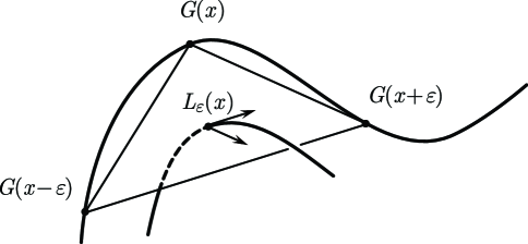
Figure 4: The envelope $L_{\epsilon}(x)$ in 3D. The point $L_{\epsilon}(x)$ and the vectors $L_{\epsilon}^{\prime}(x)$ and $L_{\epsilon}^{\prime\prime}(x)$ belong to the plane $(G(x-\epsilon),G(x),G(x+\epsilon))$.

Similarly, for even $d=2\varkappa$ the lift $L_{\epsilon}(x)$ satisfies the system of $d$ equations:

$$\det|G(x-(2\varkappa-1)\epsilon),G(x-(2\varkappa-3)\epsilon),...,G(x-\epsilon),G(x+\epsilon),...$$

$$...,G(x+(2\varkappa-1)\epsilon),L^{(j)}_{\epsilon}(x)|=0,\quad j=0,...,d-1.$$ (4)

The evolution of the curve $\gamma$ in the direction of the envelope $\ell_{\epsilon}$, as $\epsilon$ changes, defines a continuous limit of the pentagram map $T$. Namely, below we show that the expansion of $L_{\epsilon}(x)$ has the form

$$L_{\epsilon}(x)=G(x)+\epsilon^{2}B(x)+{\mathcal{O}}(\epsilon^{4}).$$

The family of functions $L_{\epsilon}(x)$ satisfies a family of differential equations:

$$L_{\epsilon}^{(d+1)}+u_{d-1,\epsilon}(x)L_{\epsilon}^{(d-1)}+...+u_{1,\epsilon}(x)L_{\epsilon}^{\prime}+u_{0,\epsilon}(x)L_{\epsilon}=0,$$

where $u_{j,0}(x)=u_{j}(x).$

Expanding the coefficients $u_{j,\epsilon}(x)$ as $u_{j,\epsilon}(x)=u_{j}(x)+\epsilon^{2}w_{j}(x)+{\mathcal{O}}(\epsilon^{4})$, we define the continuous limit of the pentagram map $T$ as the system of evolution differential equations $du_{j}(x)/dt\,=w_{j}(x)$ for $j=0,...,d-1$, i.e., $\epsilon^{2}$ plays the role of time.

Theorem A. The continuous limit $du_{j}(x)/dt\,=w_{j}(x),\,j=0,...,d-1$ for $x\in S^{1}$ of the pentagram map is the $(2,d+1)$-KdV equation of the Adler-Gelfand-Dickey hierarchy on the circle.

This theorem is proved as a combination of Theorems 4.3 and 4.5 below.

Remark 4.1.

Recall the definition of the KdV hierarchy (after Adler-Gelfand-Dickey, [1]). Let $L$ be a linear differential operator of order $d+1$:

$$L=\partial^{d+1}+u_{d-1}(x)\partial^{d-1}+u_{d-2}(x)\partial^{d-2}+...+u_{1}(x)\partial+u_{0}(x)$$ (5)

with periodic coefficients $u_{j}(x)$, where $\partial^{k}$ stands for $d^{k}/dx^{k}$. One can define its fractional power $L^{m/{d+1}}$ as a pseudo-differential operator for any positive integer $m$ and take its purely differential part $Q_{m}:=(L^{m/{d+1}})_{+}$ . In particular, for $m=2$ one has $Q_{2}=\partial^{2}+\dfrac{2}{d+1}u_{d-1}(x)$. Then the $(m,d+1)$-KdV equation is the following evolution equation on (the coefficients of) $L$:

$$\frac{d}{dt}{L}=[Q_{m},L]\,.$$

Remark 4.2.

a) For $d=1$ the discrete pentagram map is the identity map, hence the continuous limit is trivial, which is consistent with vanishing of the (2,2)-KdV equation.

b) For $d=2$ the (2,3)-KdV equation is the classical Boussinesq equation, found in [11].

c) Apparently, the $(2,d+1)$-KdV equation is a very robust continuous limit. One obtains it not only for the pentagram map defined by taking every other vertex, but also for a non-symmetric choice of vertices for the plane $P_{k}$, see Remark 4.4. Also, the limit remains the same if instead of taking the envelopes one starts with a map defined by taking intersections of various planes [9].

4.2 Envelopes and the KdV hierarchy

Theorem 4.3.

For any dimension $d$, the envelope $L_{\epsilon}(x)$ has the expansion

$$L_{\epsilon}(x)=G(x)+{\epsilon^{2}}\,C_{d}\left(G^{\prime\prime}(x)+\dfrac{2}{d+1}u_{d-1}G(x)\right)+{\mathcal{O}}(\epsilon^{4})$$

for a certain constant $C_{d}$, as $\epsilon\to 0$.

The $\epsilon^{2}$-term of this expansion can be rewritten as $C_{d}\left(\partial^{2}+\dfrac{2}{d+1}u_{d-1}(x)\right)G(x).$ Consequently, it defines the following evolution of the curve $G(x)$:

$$\frac{d}{dt}G=\left(\partial^{2}+\dfrac{2}{d+1}u_{d-1}\right)G.$$

Proof.

Since $L_{\epsilon}$ approaches $G$ as $\epsilon\to 0$, one has the expansion $L_{\epsilon}=G+\epsilon A+\epsilon^{2}B+\epsilon^{3}C+{\mathcal{O}}(\epsilon^{4}).$ First we note that the expansion of $L_{\epsilon}$ in $\epsilon$ has only even powers of $\epsilon$, since the equations (3) and (4) defining $L_{\epsilon}$ have the symmetry $\epsilon\to-\epsilon$. Therefore, we have $A=C=0$ and $L_{\epsilon}=G+\epsilon^{2}B+{\mathcal{O}}(\epsilon^{4}).$

Notice that $G(x)$ with its first $d$ derivatives form a basis in ${\mathbb{R}}^{d+1}$ for each $x$. We express the vector coefficient $B$ in this basis: $B=b_{0}(x)G+b_{1}(x)G^{\prime}+...+b_{d}(x)G^{(d)}$. Recall that, e.g., for odd $d=2\varkappa+1$ the lift $L_{\epsilon}(x)$ satisfies the system of $d$ equations:

$$\det|\,G(x-\varkappa\epsilon),G(x-(\varkappa-1)\epsilon),...,G(x),...,G(x+\varkappa\epsilon),L^{(j)}_{\epsilon}(x)\,|=0,\quad j=0,...,d-1.$$

Fix $x$ and expand all terms in $\epsilon$: e.g., $G(x+\epsilon)=G(x)+\epsilon G^{\prime}(x)+\frac{\epsilon^{2}}{2}G^{\prime\prime}+...$, etc. In each equation consider the coefficients at the lowest power of $\epsilon$, being $2+{d(d-1)}/{2}$ here.

The equation with $j=0$ gives $C_{d}\det|G,G^{\prime},...,G^{(d-1)},B|=0$ for some nonzero $C_{d}$, which implies that there is no $G^{(d)}$-term in the expansion of $B$. Similarly, for $j=1$ we obtain $C_{d}\det|G,G^{\prime},...,G^{(d-1)},B^{\prime}|=0$, which means that there is no $G^{(d)}$-term in the expansion of $B^{\prime}$, or, equivalently, there is no $G^{(d-1)}$-term in the expansion of $B$. Using this argument for $j=0,1,...,d-3,$ and $d-1$, we deduce that $B$ contains no terms with $G^{(d)},...,G^{\prime\prime\prime}$ and $G^{\prime}$.

The equation with $j=d-2$ results in a different term in the expansion and gives

$$\det|G,G^{\prime},...,G^{(d-1)},B^{(d-2)}|=C_{d}\,\det|G,G^{\prime},...,G^{(d-1)},G^{(d)}|\,,$$

which implies that $B=C_{d}G^{\prime\prime}+b(x)G$ for some function $b(x)$.

Finally, the normalization $\det|\,L_{\epsilon},L^{\prime}_{\epsilon},...,L^{(d)}_{\epsilon}\,|=1$ allows one to find $b(x)$ by plugging in it $L_{\epsilon}=G+\epsilon^{2}(C_{d}G^{\prime\prime}+b(x)G)+{\mathcal{O}}(\epsilon^{4}).$ For the $\epsilon^{2}$-terms one obtains

$$C_{d}\det|\,G,G^{\prime},...,G^{(d-2)},G^{(d+1)},G^{(d)}\,|+C_{d}\det|\,G,G^{\prime},...,G^{(d-2)},G^{(d-1)},G^{(d+2)}\,|$$

$$+(d+1)b(x)\det|\,G,G^{\prime},...,G^{(d-2)},G^{(d-1)},G^{(d)}\,|=0\,.$$

By using the linear differential equation $G^{(d+1)}+u_{d-1}(x)G^{(d-1)}+...+u_{0}(x)G=0$ to express $G^{(d+1)}$ and $G^{(d+2)}$ via lower derivatives we see that the first and the second determinants are equal to $-u_{d-1}$, while the last one is equal to 1. Thus one has $(d+1)b(x)-2C_{d}\,u_{d-1}(x)=0$, which gives $b(x)=C_{d}\frac{2}{d+1}u_{d-1}(x)$.

Hence $L_{\epsilon}=G+\epsilon^{2}\,C_{d}\,(G^{\prime\prime}+\frac{2}{d+1}u_{d-1}G)+{\mathcal{O}}(\epsilon^{4})$, as required. $\Box$

Remark 4.4.

One can see that the only condition on vertices defining the hyperplane $P_{k}$ required for the proof above is that they are distinct. A different choice of vertices for the hyperplane $P_{k}$ changes the constant $C_{d}$, but does not affect the evolution equation for $G$. The above theorem for an envelope $L_{\epsilon}(x)$ is similar to an analogous expansion in [9] for a curve defined via certain plane intersections.

Theorem 4.5.

In any dimension $d$ the continuous limit of the pentagram map defined by the evolution

$$\frac{d}{dt}G=\left(\partial^{2}+\dfrac{2}{d+1}u_{d-1}\right)G$$

of the curve $G$ coincides with the $(2,d+1)$-KdV equation. Consequently, it is an infinite-dimensional completely integrable system.

Proof.

Recall that the $(2,d+1)$-KdV equation is defined as the evolution

$$\dot{L}=[Q_{2},L]:=Q_{2}L-LQ_{2},$$

where the linear differential operator $L$ of order $d+1$ is given by formula (5) and $Q_{2}=\partial^{2}+\dfrac{2}{d+1}u_{d-1}$. Here $\dot{L}$ stands for $dL/dt$.

By assumption, the evolution of the curve $G$ is described by the differential equation $\dot{G}=Q_{2}G$. We would like to find the evolution of the operator $L$ tracing it. For any $t$, the curve $G$ and the operator $L$ are related by the differential equation $LG=0$ of order $d+1$. Consequently,

$$\dot{L}G+L\dot{G}=0.$$

Note that if the operator $L$ satisfies the $(2,d+1)$-KdV equation and $G$ satisfies $\dot{G}=Q_{2}G$, we have the identity:

$$\dot{L}G+L\dot{G}=(Q_{2}L-LQ_{2})G+LQ_{2}G=Q_{2}LG=0\,.$$

In virtue of the uniqueness of the linear differential operator of the form (5) for a given fundamental set of solutions, we obtain that indeed the evolution of $L$ is described by the $(2,d+1)$-KdV equation. $\Box$

Remark 4.6.

The proof above is reminiscent of the one used in [10] to study symplectic leaves of the Gelfand-Dickey brackets. Note that the absence of the term linear in $\epsilon$ is related to the symmetric choice of vertices for the hyperplane $P_{k}$. For a non-symmetric choice the evolution would be defined by the linear term in $\epsilon$ and given by the equation $\dot{G}=G^{\prime}$. This is the initial, $(1,d+1)$-equation of the corresponding KdV hierarchy, manifesting the fact that the space $x$-variable can be regarded as the “first time” variable. A natural question arises whether the whole KdV-hierarchy is hidden as an appropriate limit of the pentagram map. An evidence to this is given by noticing that the terms with higher powers in $\epsilon$ lead to equations similar to the higher equations in the KdV hierarchy, see Appendix 9.2.

Remark 4.7.

One can see that the continuous limit of the general pentagram maps $T_{p,r}$ for various $p\not=r$ in ${\mathbb{RP}}^{d}$ defined via envelopes for a centered choice of vertices is the same $(2,d+1)$-KdV flow, i.e., the limit depends only on the dimension.

Indeed, an analog of the $p$-diagonal is the plane $P_{\epsilon}(x)$ passing through the points $G(x),G(x+\epsilon p),...,G(x+\epsilon(d-1)p)$. Rescaling $\epsilon$, we can assume the points to be $G(x),G(x+\epsilon),...,G(x+\epsilon(d-1))$, which leads to the planes $P_{\epsilon}(x)$ defined in Section 4.1 after a shift in $x$. Then the definition of $L_{\epsilon}(x)$ via the envelope of such planes will give the same $(2,d+1)$-KdV equation.

It would be interesting to define the limit of the intersections of every $r$th plane via some higher-order terms of the envelope, as mentioned in the above remark, so that it could lead to other $(m,d+1)$-equations in the KdV hierarchy.

5 Explicit formulas for the 3D pentagram map

5.1 Two involutions

Now we return to the 3D case. In this section we assume that $n$ is odd and consider $n$-gons in ${\mathbb{RP}}^{3}$. Recall that in this case an $n$-gon with a given monodromy $M\in SL(4,{\mathbb{R}})$ lifts uniquely to ${\mathbb{R}}^{4}$ and is described by difference equations

$$V_{j+4}=a_{j}V_{j+3}+b_{j}V_{j+2}+c_{j}V_{j+1}-V_{j},\quad j\in{\mathbb{Z}},$$ (6)

with $n$-periodic coefficients $(a_{j},b_{j},c_{j})$. In other words, for odd $n$ the variables $(a_{j},b_{j},c_{j}),\;0\leq j\leq n-1,$ provide coordinates on the space $\mathcal{P}_{n}$ of twisted $n$-gons in ${\mathbb{RP}}^{3}$ considered up to projective equivalence (see Proposition 5.9).

In order to find explicit formulas for the pentagram map, we present it as a composition of two involutions $\alpha$ and $\beta$, cf. Section 3.3, and then find the formulas for each of them separately. The same approach was used in [11] in 2D, although the formulas in 3D are more complicated.

Definition 5.1.

Given a sequence of points $\phi(j)\in{\mathbb{RP}}^{3},\;j\in{\mathbb{Z}},$ define two sequences $\alpha(\phi(j))\in({\mathbb{P}}^{3})^{*}$ and $\beta(\phi(j))\in({\mathbb{RP}}^{3})^{*}$, where

$a)$ $\alpha(\phi(j))$ is the plane $(\phi(j-1),\phi(j),\phi(j+1))$;

$b)$ $\beta(\phi(j))$ is the plane $(\phi((j-2),\phi(j),\phi(j+2))$.

Proposition 5.2.

The maps $\alpha$ and $\beta$ are involutions, i.e., $\alpha^{2}=\beta^{2}=\rm{Id}$, while the pentagram map is their composition: $T=\alpha\circ\beta$.

Note that the indices which define the planes are symmetric with respect to $j$. As a result, we do not have an extra shift of indices, cf. Proposition 3.11 (unlike the 2D case and the general map $\alpha_{p}$).

Lemma 5.3.

The involution $\alpha:V_{i}\to W_{i}=*(V_{i}\wedge V_{i-1}\wedge V_{i+1})$ maps equation (6) to the following difference equation:

$$W_{i+4}=c_{i+1}W_{i+3}+b_{i}W_{i+2}+a_{i-1}W_{i+1}-W_{i}.$$

Lemma 5.4.

The involution $\beta:V_{i}\to W_{i}=\lambda_{i}*(V_{i}\wedge V_{i-2}\wedge V_{i+2})$ maps equation (6) to the difference equation

$$W_{i+4}=A_{i}W_{i+3}+B_{i}W_{i+2}+C_{i}W_{i+1}-W_{i},$$

where the coefficients $A_{i},B_{i},C_{i}$ are defined as follows:

$$A_{i} =c_{i-1}(a_{i}a_{i+2}+a_{i+2}b_{i+1}c_{i}+c_{i}c_{i+2})^{2}\lambda_{i+1}\lambda_{i+2}\lambda_{i+4}^{2},$$

$$B_{i} =((a_{i-2}+b_{i-1}c_{i-2})(c_{i+2}+a_{i+2}b_{i+1})-a_{i+2}c_{i-2})\times$$

$$\times(a_{i-1}a_{i+1}+a_{i+1}b_{i}c_{i-1}+c_{i-1}c_{i+1})\lambda_{i}\lambda_{i+1}\lambda_{i+3}\lambda_{i+4},$$

$$C_{i} =a_{i+1}(a_{i}a_{i+2}+a_{i+2}b_{i+1}c_{i}+c_{i}c_{i+2})^{2}\lambda_{i+2}\lambda_{i+3}\lambda_{i+4}^{2}.$$

The sequence $\lambda_{i},\;i\in{\mathbb{Z}},$ is $n$-periodic and is uniquely determined by the condition

$$\lambda_{i}\lambda_{i+1}\lambda_{i+2}\lambda_{i+3}=\dfrac{1}{(a_{i-2}a_{i}+a_{i}b_{i-1}c_{i-2}+c_{i-2}c_{i})(a_{i-1}a_{i+1}+a_{i+1}b_{i}c_{i-1}+c_{i-1}c_{i+1})}.$$

The proofs of these lemmas are straightforward computations, which we omit. Combined together, these lemmas provide formulas for the pentagram map. They have, however, one drawback: one needs to solve a system of equations in $\lambda_{i},\;i\in{\mathbb{Z}},$ which results in the non-local character of the formulas in $(a,b,c)$-coordinates and their extreme complexity.

5.2 Cross-ratio type coordinates

Similarly to the 2D case, there exist alternative coordinates on the space $\mathcal{P}_{n}$. They are defined for any $n$, and the formulas for the pentagram map become local, i.e., involving the vertex $\phi(j)$ itself and several neighboring ones.

Definition 5.5.

For odd $n$ the variables

$$x_{j}=\dfrac{b_{j+1}}{a_{j}a_{j+1}},\quad y_{j}=\dfrac{a_{j}}{b_{j+1}c_{j}},\quad z_{j}=\dfrac{c_{j+1}}{a_{j+1}b_{j}},\quad 0\leq j\leq n-1,$$

provide coordinates on the space $\mathcal{P}_{n}$, where the $n$-periodic variables $(a_{j},b_{j},c_{j}),\;j\in{\mathbb{Z}},$ are defined by the difference equation (6).

It turns out that the variables $(x_{j},y_{j},z_{j}),\;0\leq j\leq n-1$ are well defined and independent for any $n$, even or odd. Below we provide two (equivalent) ways to define them for even $n$: a pure geometric (local) definition of these variables (see Proposition 5.7) and the above definition extended to quasi-periodic sequences $(a_{j},b_{j},c_{j})$ (see Section 5.3).

Theorem 5.6.

In the coordinates $x_{i},y_{i},z_{i}$ the pentagram map for any (either odd or even) $n$ is given by the formulas:

$$T^{*}(x_{i}) =x_{i+1}\dfrac{1+y_{i-1}+z_{i+2}+y_{i-1}z_{i+2}-y_{i+1}z_{i}}{1+y_{i-1}+z_{i}},$$

$$T^{*}(y_{i}) =\dfrac{x_{i-1}y_{i-1}z_{i}}{x_{i}z_{i-1}}\dfrac{(1+y_{i+1}+z_{i+2})(1+y_{i-2}+z_{i-1})}{(1+y_{i}+z_{i+1})(1+y_{i-1}+z_{i+2}+y_{i-1}z_{i+2}-y_{i+1}z_{i})},$$

$$T^{*}(z_{i}) =\dfrac{x_{i+1}z_{i}}{x_{i}}\dfrac{(1+y_{i+1}+z_{i+2})(1+y_{i-2}+z_{i-1})}{(1+y_{i-1}+z_{i})(1+y_{i-2}+z_{i+1}-y_{i}z_{i-1}+y_{i-2}z_{i+1})}.$$

Before proving this theorem we describe the $(x_{i},y_{i},z_{i})$ coordinates in greater detail. It turns out that they may be defined completely independently of $(a_{i},b_{i},c_{i})$ in the following geometric way.

Recall that the $x,y$ coordinates for the 2D pentagram map are defined as cross-ratios for quadruples of points on the line $(V_{i},V_{i+1})$, where two points are these vertices themselves, and two others are intersections of this line with extensions of the neighbouring edges. Similarly, the next proposition describes the new coordinates via cross-ratios of quadruples of points, $2$ of which are the vertices of an edge, and $2$ others are the intersection of the edge extension with two planes. For instance, the variable $y_{i}$ is the cross-ratio of 4 points on the line $(V_{i},V_{i+1})$, two of which are $V_{i}$ and $V_{i+1}$, while two more are constructed as intersections of this line with the planes via the triple $(V_{i+2},V_{i+3},V_{i+4})$ and with the plane via the triple $(V_{i+2},V_{i+4},V_{i+5})$. More precisely, the following proposition holds.

Proposition 5.7.

The coordinates $x_{i},y_{i},z_{i}$ are given by the cross-ratios:

$$x_{i} =-[V_{i+4},V_{i+5},\Phi^{45}_{012},\Phi^{45}_{123}],$$

$$y_{i} =-[V_{i},V_{i+1},\Phi^{01}_{234},\Phi^{01}_{245}],$$

$$z_{i} =-[V_{i+4},V_{i+5},\Phi^{45}_{013},\Phi^{45}_{123}],$$

where the point $\Phi^{j_{1},j_{2}}_{m_{1},m_{2},m_{3}}$ for a given $i$ is the intersection of the line $(V_{i+j_{1}},V_{i+j_{2}})$ with the plane $(V_{i+m_{1}},V_{i+m_{2}},V_{i+m_{3}})$.

By the very definition these coordinates are projectively invariant.

Proof of proposition.

If $*$ is the Hodge star operator with respect to the Euclidean metric in ${\mathbb{R}}^{4}\,(\,\mathrm{or~{}}{\mathbb{C}}^{4})$, then

$$\Phi^{j_{1},j_{2}}_{m_{1},m_{2},m_{3}}=*\left(*(V_{i+j_{1}}\wedge V_{i+j_{2}})\wedge*(V_{i+m_{1}}\wedge V_{i+m_{2}}\wedge V_{i+m_{3}})\right).$$

It suffices to prove the proposition in the case of an odd $n$, because the formulas are local, and we can always add a vertex to change the parity of $n$. Therefore, we may assume that $(a_{j},b_{j},c_{j})$ are global coordinates and use them for the proof.

A simple computation shows that

$$\Phi^{45}_{012} =-(b_{i+1}+a_{i}a_{i+1})V_{i+4}+a_{i}V_{i+5},$$

$$\Phi^{01}_{234} =V_{i}-c_{i}V_{i+1},$$

$$\Phi^{01}_{245} =-b_{i+1}V_{i}+(a_{i}+c_{i}b_{i+1})V_{i+1},$$

$$\Phi^{45}_{013} =(c_{i+1}+b_{i}a_{i+1})V_{i+4}-b_{i}V_{i+5},$$

$$\Phi^{45}_{123} =-a_{i+1}V_{i+4}+V_{i+5}.$$

Recall (see Lemma 4.5 in [11]) that if $4$ vectors $a,b,c,d\in{\mathbb{R}}^{4}\,(\mathrm{or~{}}{\mathbb{C}}^{4})$ lie in the same 2-dimensional plane and are such that

$$c=\lambda_{1}a+\lambda_{2}b,\quad d=\mu_{1}a+\mu_{2}b,$$

then the cross-ratio of the lines spanned by these vectors in the plane is given by

$$[a,b,c,d]=\dfrac{\lambda_{2}\mu_{1}-\lambda_{1}\mu_{2}}{\lambda_{2}\mu_{1}}.$$

Comparing the cross-ratios with the original definition of the variables $x_{i},y_{i},z_{i}$ concludes the proof. $\Box$

Now we are in a position to prove the explicit local formulas in Theorem 5.6. The proof is similar, but more involved than that of Proposition 4.11 in [11].

Proof of theorem.

Due to the local character of the formulas for the pentagram map $T$ in $(x_{j},y_{j},z_{j})$-coordinates, we may always add an extra vertex to make the number $n$ of vertices odd, and then use coordinates $(a_{j},b_{j},c_{j})$ and Lemmas 5.3 and 5.4 for the proof.

The pentagram map is a composition $T=\alpha\circ\beta:V_{i}\to U_{i}$. Namely,

$$U_{i}=\mu_{i}*\left[*(V_{i-3}\wedge V_{i-1}\wedge V_{i+1})\wedge*(V_{i-2}\wedge V_{i}\wedge V_{i+2})\wedge*(V_{i-1}\wedge V_{i+1}\wedge V_{i+3})\right],$$

where the constants $\mu_{i}$ are chosen so that $\det|U_{j},U_{j+1},U_{j+2},U_{j+3}|=1$ for all $j$.

At the level of the coordinates $(a_{j},b_{j},c_{j})$, we obtain:

$$T^{*}(x_{i})=\dfrac{B_{i+1}}{C_{i+1}C_{i+2}},\quad T^{*}(y_{i})=\dfrac{C_{i+1}}{B_{i+1}A_{i-1}},\quad T^{*}(z_{i})=\dfrac{A_{i}}{C_{i+2}B_{i}},$$

where $A_{i},B_{i},C_{i}$ are defined in Lemma 5.4. Eliminating the variables $\lambda_{i}$ with different $i$ by using the formula for the product $\lambda_{i}\lambda_{i+1}\lambda_{i+2}\lambda_{i+3}$ concludes the proof. $\Box$

5.3 Coordinates on twisted polygons: odd vs. even $n$

In this section we compare how one introduces the coordinates on the space $\mathcal{P}_{n}$ of twisted $n$-gons for odd or even $n$, and how this changes the statements above.

Definition 5.8.

Call a sequence $(a_{j},b_{j},c_{j}),\;j\in{\mathbb{Z}}$, $n$-quasiperiodic if there is a sequence $t_{j},\;j\in{\mathbb{Z}}$, satisfying $t_{j}t_{j+1}t_{j+2}t_{j+3}=1$ and such that

$$a_{j+n}=a_{j}\dfrac{t_{j}}{t_{j+3}},\quad b_{j+n}=b_{j}\dfrac{t_{j}}{t_{j+2}},\quad c_{j+n}=c_{j}\dfrac{t_{j}}{t_{j+1}}$$ (7)

for each $j\in{\mathbb{Z}}$.

Note that a sequence $t_{j},\;j\in{\mathbb{Z}},$ must be 4-periodic, and it is defined by three parameters, e.g., by $\alpha:=t_{0}/t_{3},\,\beta:=t_{0}/t_{2},$ and $\gamma:=t_{0}/t_{1}$ with $\alpha\beta\gamma>0$, and hence $t_{0}=(\alpha\beta\gamma)^{1/4}$. Thus the space ${\mathcal{Q}S}_{n}$ of $n$-quasiperiodic sequences has dimension $3n+3$, and $\{(a_{j},b_{j},c_{j}),\;j=0,...,n-1\}\times(\alpha,\beta,\gamma)$ are coordinates on it.

Now we associate a sequence of vectors $V_{j}\in{\mathbb{R}}^{4},\;j\in{\mathbb{Z}},$ and difference equations

$$V_{j+4}=a_{j}V_{j+3}+b_{j}V_{j+2}+c_{j}V_{j+1}-V_{j},\quad j\in{\mathbb{Z}},$$ (8)

to each twisted $n$-gon $v_{j}:=\phi(j)\in{\mathbb{RP}}^{3},j\in{\mathbb{Z}},$ with a monodromy $M\in SL(4,{\mathbb{R}})$. This gives a correspondence between sequences $(a_{j},b_{j},c_{j}),\;j\in{\mathbb{Z}},$ and twisted $n$-gons.

Proposition 5.9.

There is a one-to-one correspondence between twisted $n$-gons (defined up to projective equivalence) and three-parameter equivalence classes in the space ${\mathcal{Q}S}_{n}$ of $n$-quasiperiodic sequences $\{(a_{j},b_{j},c_{j}),\;j=0,...,n-1\}\times(\alpha,\beta,\gamma)$.

If $n$ is odd, there exists a unique $n$-periodic sequence $(a_{j},b_{j},c_{j})$ in each class.

If $n=4p$, then the numbers $\alpha,\beta,\gamma$ are projective invariants of a twisted $n$-gon.

If $n=4p+2$, then there is one projective invariant: $\alpha\gamma/\beta$.

In other words, for odd $n$ the equivalence classes are “directed along” the parameters $(\alpha,\beta,\gamma)$ and one can chose a representative with $\alpha=\beta=\gamma=1$ in each class. For $n=4p$ the classes are “directed across” these parameters, and hence the latter are fixed for any given class. The case $n=4p+2$ is in between: in a sense, two of the $(\alpha,\beta,\gamma)$-parameters and one of the $(a,b,c)$-coordinates can serve as coordinates on each equivalence class.

This proposition can be regarded as an analogue of Proposition 4.1 and Remark 4.4 in [11] for $d=2$.

Proof.

First, we construct the correspondence, and then consider what happens for different arithmetics of $n$. For a given $n$-gon $v_{k}=\phi(k)$ we construct a sequence of vertices $V_{j}\in{\mathbb{R}}^{4},\;j\in{\mathbb{Z}},$ in the following way: choose the lifts $\phi(0)\to V_{0},\;\phi(1)\to V_{1},\;\phi(2)\to V_{2}$ arbitrarily, and then determine the vectors $V_{j},\;j>2,$ and $V_{j},\;j<0,$ recursively using the condition $\det(V_{j},V_{j+1},V_{j+2},V_{j+3})=1$, which follows from equation (8).

By definition of a twisted $n$-gon, we have $\phi(j+n)=M\circ\,\phi(j)$ for each $j\in{\mathbb{Z}}$, where $M\in SL(4,{\mathbb{R}})$. Consequently, for each $j\in{\mathbb{Z}}$ there exists a number $t_{j}$, such that $V_{j+n}=t_{j}MV_{j}$, and the matrix $M$ is independent of $j$. The equation $\det(V_{j+n},V_{j+1+n},V_{j+2+n},V_{j+3+n})=1$ implies that $t_{j}t_{j+1}t_{j+2}t_{j+3}=1$ and $t_{j+4}=t_{j}$ for each $j\in{\mathbb{Z}}$. In other words, the whole sequence $\{t_{j}\}$ is determined by $t_{1},t_{2},t_{3},$ and then $t_{0}=1/t_{1}t_{2}t_{3}$. Quasiperiodic conditions (7) follow from the comparison of the equation

$$V_{j+4+n}=a_{j+n}V_{j+3+n}+b_{j+n}V_{j+2+n}+c_{j+n}V_{j+1+n}-V_{j+n}$$

with equation (8).

Now we rescale the initial three vectors: $V_{0}\mapsto k_{0}V_{0},\;V_{1}\mapsto k_{1}V_{1},\;V_{2}\mapsto k_{2}V_{2}$, where $k_{0}k_{1}k_{2}\not=0$. A different lift of the three initial vectors corresponds to a different sequence $\tilde{V}_{j}=k_{j}V_{j}$, where the sequence $k_{j},j\in{\mathbb{Z}},$ must also be $4$-periodic and satisfy $k_{0}k_{1}k_{2}k_{3}=1$. This rescaling gives the action of $({\mathbb{R}}^{*})^{3}$ on the space ${\mathcal{Q}S}_{n}$ of $n$-quasiperiodic sequences. By construction, the corresponding orbits (or equivalence classes) of sequences are in a bijection with twisted $n$-gons. The group $({\mathbb{R}}^{*})^{3}$ acts as follows:

$$t_{j}\mapsto t_{j}(k_{j}/k_{j+n}),\;a_{j}\mapsto a_{j}(k_{j}/k_{j+3}),\;b_{j}\mapsto b_{j}(k_{j}/k_{j+2}),\;c_{j}\mapsto c_{j}(k_{j}/k_{j+1}).$$

Now we have 3 cases:

• $n$ is odd. Then the above $({\mathbb{R}}^{*})^{3}$-action on $t_{0},\,t_{1},\,t_{2}$ allows one to make them all equal to 1, which corresponds to the constant sequence $\{t_{j}=1,\,j\in{\mathbb{Z}}\}$ and a periodic sequence $\{(a_{j},b_{j},c_{j}),\;j\in{\mathbb{Z}}\}$. Indeed, e.g., for $n=4p+3$ one has the system of 3 equations: $t_{0}(k_{0}/k_{3})=1,\,t_{1}(k_{1}/k_{4})=1,\,t_{2}(k_{2}/k_{5})=1$. Since $k_{4}=k_{0}$, $k_{5}=k_{1}$, and $k_{3}=1/k_{0}k_{1}k_{2}$, we obtain a system of 3 equations on the unknowns $k_{0},k_{1},k_{2}$, which has the unique solution.

• $n=4p+2$. One can check that the $({\mathbb{R}}^{*})^{3}$-action does not change the ratio $\dfrac{t_{0}t_{2}}{t_{1}t_{3}}=\dfrac{\alpha\gamma}{\beta}$.

• $n=4p$. The $({\mathbb{R}}^{*})^{3}$-action does not change the three quantities $t_{0}/t_{3},\,t_{0}/t_{2},\,t_{0}/t_{1}$. $\Box$

Now we can introduce coordinates on the space ${\mathcal{Q}S}_{n}$ of $n$-quasiperiodic sequences using Definition 5.5 and quasiperiodic variables $(a_{j},b_{j},c_{j})$.

Proposition 5.10.

For any $n$ the variables $(x_{j},y_{j},z_{j}),\;0\leq j\leq n-1$ are independent and constant on the equivalence classes in ${\mathcal{Q}S}_{n}$, i.e., they are well-defined local coordinates on the space $\mathcal{P}_{n}={\mathcal{Q}S}_{n}/\sim$.

Proof.

It is straightforward to check that the $({\mathbb{R}}^{*})^{3}$-action defined above is trivial on the variables $(x_{j},y_{j},z_{j})$. For instance,

$$x_{j}=\dfrac{b_{j+1}}{a_{j}a_{j+1}}\to\dfrac{b_{j+1}(k_{j+1}/k_{j+3})}{a_{j}(k_{j}/k_{j+3})\,a_{j+1}(k_{j+1}/k_{j+4})}=x_{j}\,.$$

The independence of the new variables on ${\mathcal{Q}S}_{n}$ follows from that for the original ones. Alternatively, it also follows from their local geometric definition (Proposition 5.7). $\Box$

Remark 5.11.

In the $(a,b,c)$-coordinates for even $n$ some of the $(\alpha,\beta,\gamma)$-parameters were needed to describe the equivalence classes in ${\mathcal{Q}S}_{n}$. In the $(x,y,z)$-coordinates those parameters are functions of $x_{j},y_{j},z_{j}$:

$i)$ for $n=4p+2$,

$$\prod_{j=0}^{2p}\dfrac{x_{2j}^{2}y_{2j}z_{2j+1}}{x_{2j+1}^{2}y_{2j+1}z_{2j}}=\dfrac{\alpha\gamma}{\beta}\;;$$

$ii)$ for $n=4p$,

$$\prod_{j=0}^{p-1}\dfrac{x_{4j}x_{4j+2}y_{4j+2}z_{4j+1}}{x_{4j+1}x_{4j+3}y_{4j+3}z_{4j+2}}=\alpha,\quad\prod_{j=0}^{p-1}\dfrac{y_{4j+1}z_{4j}}{y_{4j+3}z_{4j+2}}=\beta,\quad\prod_{j=0}^{p-1}\dfrac{y_{4j}z_{4j+3}}{y_{4j+2}z_{4j+1}}=\frac{\gamma}{\alpha}\,.$$

These identities follow from Definitions 5.5 and 5.8.

6 Algebraic-geometric integrability of the 3D pentagram map

In this section we complexify the pentagram map and assume that everything is defined over ${\mathbb{C}}$.

6.1 Scaling transformations and a Lax function in 3D

Recall that a discrete Lax equation with a spectral parameter is a representation of a dynamical system in the form

$$L_{i,t+1}(\lambda)=P_{i+1,t}(\lambda)L_{i,t}(\lambda)P_{i,t}^{-1}(\lambda),$$ (9)

where $t$ stands for the discrete time variable, $i$ refers to the vertex index, and $\lambda$ is a complex spectral parameter.

The pivotal property responsible for algebraic-geometric integrability of all pentagram maps considered in this paper is the presence of a scaling invariance. In the 2D case, this means the invariance with respect to the transformations $a_{j}\to a_{j}s,\;b_{j}\to b_{j}/s$, where $s$ is an arbitrary number. In the 3D case, the pentagram map is invariant with respect to the transformations $a_{j}\to a_{j}s,\;b_{j}\to b_{j},\;c_{j}\to c_{j}s$. In both cases the invariance follows from the explicit formulas of the map. Note that formally one can define other pentagram maps by choosing the intersection planes in many different ways. However, only very few of these maps possess any scaling invariance. Below we derive a Lax representation from the scaling invariance. First we do it for odd $n$, when $(a_{j},b_{j},c_{j}),0\leq j\leq n-1,$ are coordinates on the space ${\mathcal{P}}_{n}$.

Theorem 6.1.

The 3D pentagram map on twisted $n$-gons with odd $n$ admits a Lax representation with the Lax function $L_{j}(\lambda)$ given by

$$L_{j}(\lambda)=\begin{pmatrix}c_{j}/\lambda&1/\lambda&0&0\\ b_{j}&0&1&0\\ a_{j}/\lambda&0&0&1/\lambda\\ -1&0&0&0\end{pmatrix}=\begin{pmatrix}0&0&0&-1\\ \lambda&0&0&c_{j}\\ 0&1&0&b_{j}\\ 0&0&\lambda&a_{j}\end{pmatrix}^{-1}$$

in the coordinates $a_{j},b_{j},c_{j}$. Its determinant is $\det{L_{j}}\equiv 1/\lambda^{2}$.

Note that we always consider a polygon and the corresponding Lax function at a particular moment of time. Whenever necessary we indicate the moment of time explicitly by adding the second index “$t$” to the Lax function (above $L_{j}:=L_{j,t}$), while if there is no ambiguity we keep only one index. Before proving this theorem we give the following

Definition 6.2.

The monodromy operators $T_{0,t},T_{1,t},...,T_{n-1,t}$ are defined as the following ordered products of the corresponding Lax functions:

$$T_{0,t}=L_{n-1,t}L_{n-2,t}...L_{0,t},$$

$$T_{1,t}=L_{0,t}L_{n-1,t}L_{n-2,t}...L_{1,t},$$

$$...$$

$$T_{i,t}=L_{i+n-1,t}L_{i+n-2,t}...L_{i+1,t}L_{i,t},$$

$$...$$

$$T_{n-1,t}=L_{n-2,t}L_{n-3,t}...L_{0,t}L_{n-1,t},$$

where the (integer) index $t$ represents the moment of time.

Proof of theorem.

First observe that the Lax equation implies that the corresponding monodromy operators satisfy

$$T_{i,t+1}(\lambda)=P_{i,t}(\lambda)T_{i,t}(\lambda)P_{i,t}^{-1}(\lambda),$$

i.e., $T_{i,t}(\lambda)$ changes to a similar matrix when $t\to t+1$, and hence the eigenvalues of the matrices $T_{i,t}(\lambda)$ as functions of $\lambda$ are invariants of the map. Conversely, if some function $T_{i,t}(\lambda)$ has this property, then there must exist a matrix $P_{i,t}(\lambda)$ (defined up to a multiplication by a scalar function) satisfying the above equation.

How to define such a monodromy depending on a parameter? The monodromy matrix associated with the difference equation

$$V_{j+4}=a_{j}V_{j+3}+b_{j}V_{j+2}+c_{j}V_{j+1}-V_{j}$$

is $M=N_{0}N_{1}N_{2}...N_{n-1}$, where

$$N_{j}=\begin{pmatrix}0&0&0&-1\\ 1&0&0&c_{j}\\ 0&1&0&b_{j}\\ 0&0&1&a_{j}\end{pmatrix}.$$

For odd $n$ the variables $(a_{j},b_{j},c_{j}),0\leq j\leq n-1,$ are well-defined coordinates on the space of twisted $n$-gons. These variables are periodic: for any $j$ we have $a_{j+n}=a_{j},\;b_{j+n}=b_{j},\;c_{j+n}=c_{j}$. The vectors $V_{j}$ are quasi-periodic: $V_{j+n}=MV_{j}$, and depend on the lift of the points from the projective space. This means that the pentagram map preserves the eigenvalues of the matrix $M$, but not the matrix $M$ itself.

Lemmas 5.3 and 5.4 imply that the pentagram map is invariant with respect to the scaling transformations: $a_{j}\to sa_{j},\;c_{j}\to sc_{j}$. Therefore, the pentagram map also preserves the eigenvalues of the monodromy matrix $M(s)$ corresponding to the $n$-gons scaled by $s$. Namely, we have

$$M(s)=N_{0}(s)N_{1}(s)N_{2}(s)...N_{n-1}(s),\text{ where }N_{j}(s)=\begin{pmatrix}0&0&0&-1\\ 1&0&0&sc_{j}\\ 0&1&0&b_{j}\\ 0&0&1&sa_{j}\end{pmatrix}.$$

Now one can see that the matrix $N_{j}(s)$ can be chosen as a Lax function. For technical reasons (which will be clear later), we define the Lax matrix as $L_{j}^{-1}(\lambda):=(g^{-1}N_{j}(s)g)/s$, where $g:=\text{diag}(1,s,1,s)$, and $\lambda:=1/s^{2}$. This gives the required matrix $L_{j}(\lambda)$. $\Box$

As we mentioned before, the formulas for the pentagram map are non-local in the variables $(a_{j},b_{j},c_{j})$. As a result, an explicit expression for the matrix $P_{i,t}(\lambda)$ becomes non-local as well. On the other hand, one can use the variables $(x_{j},y_{j},z_{j})$ (given by Definition 5.5) to describe a Lax representation. Their advantage is that all formulas become local and are valid for any $n$, both even and odd.

Theorem 6.3.

For any $n$ the equations for the 3D pentagram map are equivalent to the Lax equation

$$\tilde{L}_{i,t+1}(\lambda)=\tilde{P}_{i+1,t}(\lambda)\tilde{L}_{i,t}(\lambda)\tilde{P}_{i,t}^{-1}(\lambda),$$

where

$$\tilde{L}_{i,t}(\lambda)=\begin{pmatrix}0&0&0&-1\\ \lambda x_{i}y_{i}&0&0&1\\ 0&z_{i}&0&1\\ 0&0&\lambda x_{i}&1\end{pmatrix}^{-1},$$

$$\tilde{P}_{i,t}(\lambda)=\begin{pmatrix}0&\rho_{i}&0&-\rho_{i}\\ \lambda\sigma_{i}(1+z_{i})&-\rho_{i}&\lambda\sigma_{i}&\rho_{i}\\ y_{i-1}\theta_{i}&\dfrac{z_{i-1}}{\tau_{i}}&-\theta_{i}&\dfrac{1+y_{i-2}}{\tau_{i}}\\ -\dfrac{\lambda y_{i-1}}{1+y_{i-1}+z_{i}}&0&\dfrac{\lambda}{1+y_{i-1}+z_{i}}&0\end{pmatrix},$$

and the variables $\rho_{i},\sigma_{i},\tau_{i},$ and $\theta_{i}$ stand for

$$\rho_{i} =\dfrac{1}{x_{i}(1+y_{i}+z_{i+1})},$$

$$\sigma_{i} =\dfrac{x_{i-1}y_{i-1}(1+y_{i-2}+z_{i-1})}{x_{i}z_{i-1}(1+y_{i-1}+z_{i})(1+y_{i}+z_{i+1})},$$

$$\tau_{i} =x_{i}(1+y_{i-2}-y_{i}z_{i-1}+z_{i+1}+z_{i+1}y_{i-2}),$$

$$\theta_{i} =\dfrac{1+y_{i-2}+z_{i-1}}{\tau_{i}(1+y_{i-1}+z_{i})}.$$

Proof.

The proof is a long but straightforward verification. $\Box$

Remark 6.4.

The Lax functions $L$ and $\tilde{L}$ in the $(a_{i},b_{i},c_{i})$ and $(x_{i},y_{i},z_{i})$ variables are related to each other as follows:

$$\tilde{L}_{i,t}=a_{i+1}\left(h_{i+1}^{-1}L_{i,t}h_{i}\right),\text{ where }h_{i}:=\text{diag}(1,c_{i},b_{i},a_{i}).$$

6.2 Properties of the spectral curve

Recall that the monodromy operators $T_{i,t}(\lambda)$ satisfy the equation

$$T_{i,t+1}(\lambda)=P_{i,t}(\lambda)T_{i,t}(\lambda)P_{i,t}^{-1}(\lambda).$$

It implies that the function of two variables $R(\lambda,k)=\det{(T_{i,t}(\lambda)-k\,\text{Id})}$ is independent of $i$ and $t$. Furthermore, $R(\lambda,k)=0$ is a polynomial relation between $\lambda$ and $k$: $R(\lambda,k)$ becomes a polynomial after a multiplication by a power of $\lambda$. Its coefficients are integrals of motion for the pentagram map. The zero set of $R(\lambda,k)=0$ is an algebraic curve in ${\mathbb{C}}^{2}$. A standard procedure (of adding the infinite points and normalization with a few blow-ups) makes it into a compact Riemann surface, which we call the spectral curve and denote by $\Gamma$. In this section we explore some of the properties of the spectral curve and, in particular, find its genus.

Definition 6.5.

For an odd $n$ define the spectral function $R(\lambda,k)$ as

$$R(\lambda,k):=\det{(T_{i,t}(\lambda)-k\,\text{Id})},$$

i.e., using the Lax function in the $(a,b,c)$-coordinates from Theorem 6.1. The spectral curve $\Gamma$ is the normalization of the compactification of the curve $R(\lambda,k)=0$.

We define the integrals of motion $I_{j},J_{j},G_{j},\;0\leq j\leq q=\lfloor n/2\rfloor,$ as the coefficients of the expansion

$$R(\lambda,k)=k^{4}-k^{3}\left(\sum_{j=0}^{q}G_{j}\lambda^{j-n}\right)+k^{2}\left(\sum_{j=0}^{q}J_{j}\lambda^{j-q-n}\right)-k\left(\sum_{j=0}^{q}I_{j}\lambda^{j-2n}\right)+\lambda^{-2n}=0.$$

When $n$ is even, the sequence $(a_{j},b_{j},c_{j}),\;j\in{\mathbb{Z}}$, is not $n$-periodic, and the monodromy operator $T_{i,t}(\lambda)$ cannot be defined. One should use the Lax function $\tilde{L}_{i,t}(\lambda)$ in the $(x,y,z)$-coordinates from Theorem 6.3 to define the monodromy operator $\tilde{T}_{i,t}(\lambda)$ and the corresponding spectral curve.

Namely, first note that the integral of motion $I_{0}$ has the following explicit expression:

$$I_{0}=\prod_{i=0}^{n-1}a_{i}=\left(\prod_{i=0}^{n-1}x_{i}^{2}y_{i}z_{i}\right)^{-1/4}.$$

Definition 6.6.

For any $n$ (either even or odd), the spectral function is

$$R(\lambda,k)=\tilde{R}(\lambda,kI_{0})/I_{0}^{4},\;\text{ where }\;\tilde{R}(\lambda,k):=\det{(\tilde{T}_{i,t}(\lambda)-k\,\text{Id})}\,,$$

and the monodromy operator $\tilde{T}_{i,t}(\lambda)$ is defined using the Lax function $\tilde{L}_{i,t}(\lambda)$ from Theorem 6.3.

The spectral function $R(\lambda,k)$ defined this way coincides with $\det{(T_{i,t}(\lambda)-k\,\text{Id})}$ for odd $n$, since $\tilde{T}_{i,t}=I_{0}\left(h_{i}^{-1}T_{i,t}h_{i}\right)$, see Remark 6.4. It is convenient to have such a unified definition for computations of integrals of motion.

Theorem 6.7.

For generic values of the integrals of motion $I_{j},J_{j},G_{j}$, the genus $g$ of the spectral curve $\Gamma$ is $g=3q$ for odd $n$ and $g=3q-3$ for even $n$, where $q=\lfloor n/2\rfloor$.

To prove it, we first describe the singularities of $R(\lambda,k)=0$ by considering the formal series solutions (the so-called Puiseux series).

Lemma 6.8.

If $n$ is even, the equation $R(\lambda,k)=0$ has 4 formal series solutions at $\lambda=0$:

$$O_{1}:\quad k_{1} =\dfrac{1}{I_{0}}-\dfrac{I_{1}}{I_{0}^{2}}\lambda+{\mathcal{O}}(\lambda^{2}),$$

$$O_{2,3}:\quad k_{2,3} =\dfrac{k_{*}}{\lambda^{q}}+{\mathcal{O}}\left(\dfrac{1}{\lambda^{q-1}}\right),\quad\text{ where $k_{*}$ satisfies}\quad G_{0}k_{*}^{2}-J_{0}k_{*}+I_{0}=0,$$

$$O_{4}:\quad k_{4} =\dfrac{G_{0}}{\lambda^{n}}+\dfrac{G_{1}}{\lambda^{n-1}}+\dfrac{G_{2}}{\lambda^{n-2}}+{\mathcal{O}}(\lambda^{3-n}),$$

and $4$ solutions at $\lambda=\infty$:

$$W_{1,2,3,4}:\quad k_{1,2,3,4}=\dfrac{k_{\infty}}{\lambda^{q}}+{\mathcal{O}}\left(\dfrac{1}{\lambda^{q+1}}\right),\text{ where }k_{\infty}^{4}-G_{q}k_{\infty}^{3}+J_{q}k_{\infty}^{2}-I_{q}k_{\infty}+1=0.$$

If $n$ is odd, the equation $R(\lambda,k)=0$ has 4 formal series solutions at $\lambda=0$:

$$O_{1}:\quad k_{1} =\dfrac{1}{I_{0}}-\dfrac{I_{1}}{I_{0}^{2}}\lambda+{\mathcal{O}}(\lambda^{2}),$$

$$O_{2}:\quad k_{2,3} =\pm\dfrac{\sqrt{-I_{0}/G_{0}}}{\lambda^{n/2}}+\dfrac{J_{0}}{2G_{0}\lambda^{(n-1)/2}}+{\mathcal{O}}\left(\dfrac{1}{\lambda^{(n-2)/2}}\right),$$

$$O_{3}:\quad k_{4} =\dfrac{G_{0}}{\lambda^{n}}+\dfrac{G_{1}}{\lambda^{n-1}}+\dfrac{G_{2}}{\lambda^{n-2}}+{\mathcal{O}}(\lambda^{3-n}),$$

and $4$ solutions at $\lambda=\infty$:

$$W_{1,2}:\quad k_{1,2,3,4}=\dfrac{k_{\infty}}{\lambda^{n/2}}+{\mathcal{O}}\left(\dfrac{1}{\lambda^{(n+1)/2}}\right),\text{ where }k_{\infty}^{4}+J_{q}k_{\infty}^{2}+1=0.$$

The remaining coefficients of the series are determined uniquely.

Proof of lemma.

One finds the series coefficients recursively by substituting the series into the equation $R(\lambda,k)=0$, which determines the spectral curve. $\Box$

Now we can complete the proof of Theorem 6.7.

Proof of theorem.

As follows from the definition of the spectral curve $\Gamma$, it is a ramified 4-fold cover of ${\mathbb{CP}}^{1}$, since the $4\times 4$-matrix $\tilde{T}_{i,t}$ (or ${T}_{i,t}$) has 4 eigenvalues. By the Riemann-Hurwitz formula the Euler characteristic of $\Gamma$ is $\chi(\Gamma)=4\chi({\mathbb{CP}}^{1})-\nu=8-\nu$, where $\nu$ is the number of branch points. On the other hand, $\chi(\Gamma)=2-2g$, and once we know $\nu$ it allows us to find the genus of the spectral curve $\Gamma$ from the formula $2-2g=8-\nu$.

The number $\nu$ of branch points of $\Gamma$ on the $\lambda$-plane equals the number of zeroes of the function $\partial_{k}R(\lambda,k)$ aside from the singular points. The function $\partial_{k}R(\lambda,k)$ is meromorphic on $\Gamma$, therefore the number of its zeroes equals the number of its poles. One can see that for any $n$ the function $\partial_{k}R(\lambda,k)$ has poles of total order $9n$ at $z=0$, and it has zeroes of total order $6n$ at $z=\infty$. Indeed, substitute the local series from Lemma 6.8 to the expression for $\partial_{k}R(\lambda,k)$. (E.g., for $n=2q$ at $O_{4}$ one has $k\sim\lambda^{-n}$. The leading terms of $\partial_{k}R(\lambda,k)$ for the pole at $\lambda=0$ are $k^{3},k^{2}\lambda^{-n},k\lambda^{-q-n},\lambda^{-2n}$. The first two terms, being of order $\lambda^{-3n}$, dominate and give the pole order of $3n=6q$.) The corresponding orders of the poles and zeroes of $\partial_{k}R(\lambda,k)$ on $\Gamma$ are summarized as follows:

$$\begin{array}[]{||c|c||c|c||c|c||c|c||}\hline\cr n=2q&\text{ pole }&&\text{ zero }&n=2q+1&\text{ pole }&&\text{ zero }\\ \hline\cr O_{1}&4q&W_{1}&3q&O_{1}&2n&W_{1}&3n\\ \hline\cr O_{2}&4q&W_{2}&3q&O_{2}&4n&W_{2}&3n\\ \hline\cr O_{3}&4q&W_{3}&3q&O_{3}&3n&&\\ \hline\cr O_{4}&6q&W_{4}&3q&&&&\\ \hline\cr\end{array}$$

For instance, for $n=2q$ this gives the total order of poles: $4q+4q+4q+6q=18q=9n$, while the total order of zeroes is $4\times 3q=12q=6n$.

Therefore, the number of zeroes of $\partial_{k}R(\lambda,k)$ at nonsingular points $\lambda\not=\{0,\infty\}$ is $\nu=9n-6n=3n$, and so is the total number of branch points of $\Gamma$ in the finite part of the $(\lambda,k)$ plane. The difference between odd and even values of $n$ arises because $\Gamma$ has 2 additional branch points at $\lambda=\infty$, and 1 branch point at $\lambda=0$ for odd $n$, i.e., $\nu=3n+3$.

Consequently, one has $2-2g=8-\nu$ with $\nu=3n$ for even $n$ and $\nu=3n+3$ for odd $n$. The required expression for the genus $g$ follows: $g=3q-3$ for $n=2q$ and $g=3q$ for $n=2q+1$. $\Box$

Remark 6.9.

Now we describe a few integrals of motion using the coordinates $(a_{j},b_{j},c_{j}),0\leq j\leq n-1,$ when $n$ is odd. The description is similar to that in the 2D case (cf. Section 5.2 and Proposition 5.3 in [11]). Consider a code which is an ordered sequence of digits from $1$ to $4$. The number of digits in a code is $p,q,r,t$, respectively. The code is called “admissible” if $p+2q+3r+4t=n$. The number $p+r$ is called its “weight.” Each code expands in a “word” of $n$ characters in the following way: $1,2,3,4$ are replaced by “a”,“*b”,“**c”,“****”, respectively. Now we label the vertices of an $n$-gon by $0,1,...,n-1$, and associate letters in a word to them keeping the order. We obtain one monomial by taking the product of the variables $a_{i}$,$b_{i}$, or $c_{i}$ that occur at the vertex $i$. The letter “*” corresponds to “1”. The sign of the monomial is $(-1)^{t}$. Next step is to permute the numbering of the vertices cyclically and take the sum of the monomials. Note, however, that if, for example, $n=9$, then the code “333” corresponds to the sum $c_{0}c_{3}c_{6}+c_{1}c_{4}c_{7}+c_{2}c_{5}c_{8}$ without the coefficient $3$. Finally, we repeat this procedure for all admissible codes of weight $p+r$ and denote the total sum by $\hat{I}_{p+r}$. Additionally, we define the sum $\hat{G}_{p+r}$ by substituting $a_{i}\to c_{i+1},\;c_{i}\to a_{i-1}$ in $\hat{I}_{p+r}$.

Consider, for example, the case $n=7$. Then all admissible codes of weight $1$ are $142,124,1222,34,223$. The corresponding sum is

$$\hat{I}_{1}=\sum_{\text{cyclic}}(-a_{1}b_{0}-a_{5}b_{0}+a_{5}b_{0}b_{2}b_{4}-c_{0}+c_{0}b_{2}b_{4}).$$

Proposition 6.10.

For odd $n$ one has

$$I_{0}=\prod_{j=0}^{n-1}a_{j}\,,\quad I_{q}=\hat{I}_{1},\quad I_{i}=\hat{I}_{n-2i}\,,$$

$$G_{0}=\prod_{j=0}^{n-1}c_{j}\,,\quad G_{q}=\hat{G}_{1},\quad G_{i}=\hat{G}_{n-2i}\,.$$

Proof.

The proof is analogous to the proof of Proposition 5.3 in [11]. $\Box$

6.3 The spectral curve and invariant tori

The spectral curve is a crucial component of algebraic-geometric integrability. Below we always assume it to be generic. (As everywhere in this paper, “generic” means values of parameters from some Zariski open subset in the space of parameters.) It has a natural torus, its Jacobian, associated with it. It turns out that one can recover a Lax function from the spectral curve and a point on the Jacobian, and vice versa: in our situation this correspondence is locally one-to-one. The dynamics of the pentagram map becomes very simple on the Jacobian. In this section, we construct this correspondence and describe the dynamics of the pentagram map.

Definition 6.11.

A Floquet-Bloch solution $\psi_{i,t}$ of a difference equation $\psi_{i+1,t}=\tilde{L}_{i,t}\psi_{i,t}$ is an eigenvector of the monodromy operator:

$$\tilde{T}_{i,t}\psi_{i,t}=k\psi_{i,t}.$$

The normalization $\sum_{j=1}^{4}\psi_{0,0,j}\equiv 1$ (i.e., the sum of all components of the vector $\psi_{0,0}$ is equal to $1$) determines all vectors $\psi_{i,t}$ with $i,t\geq 0$ uniquely. Denote the normalized vectors $\psi_{i,t}$ by $\bar{\psi}_{i,t}$, i.e., $\bar{\psi}_{i,t}=\psi_{i,t}/\left(\sum_{j=1}^{4}\psi_{i,t,j}\right)$. (The vectors $\psi_{0,0}$ and $\bar{\psi}_{0,0}$ are identical in this notation.) We also denote by $D_{i,t}$ the pole divisor of $\bar{\psi}_{i,t}$ on $\Gamma$.

Remark 6.12.

We use the Lax function $\tilde{L}_{i,t}$ and the monodromy operator $\tilde{T}_{i,t}$ in the above definition to allow for both even and odd $n$. In the case of odd $n$ one can instead employ the Lax function $L_{i,t}$ and the monodromy operator $T_{i,t}$, while all the statements and proofs below remain valid.

Theorem 6.13.

A Floquet-Bloch solution $\bar{\psi}_{i,t}$ is a meromorphic vector function on $\Gamma$. Generically its pole divisor $D_{i,t}$ has degree $g+3$.

Proof.

The proof of the fact that the function $\bar{\psi}_{i,t}$ is meromorphic on the spectral curve $\Gamma$, as well as that its number of poles is $\deg D_{i,t}=\nu/2$, is identical to the proof of Proposition 3.4 in [15]. The number $\nu$ of the branch points of $\Gamma$ is different: in Theorem 6.7 we found that $2-2g=8-\nu$, where $g$ is the genus of the spectral curve. This implies the required expression: $\deg D_{i,t}=g+3$. $\Box$

Definition 6.14.

Let $J(\Gamma)$ be the Jacobian of the spectral curve $\Gamma$, and $[D_{0,0}]$ is the equivalence class of the divisor $D_{0,0}$, the pole divisor of $\psi_{0,0}$, under the Abel map. The pair consisting of the spectral curve $\Gamma$ (with marked points $O_{i}$ and $W_{i}$) and a point $[D_{0,0}]\in J(\Gamma)$ is called the spectral data. The spectral map $S$ associates to a given generic twisted $n$-gon in ${\mathbb{CP}}^{3}$ its spectral data $(\Gamma,[D_{0,0}])$.

The algebraic-geometric integrability is based on the following theorem.

Theorem 6.15.

For any $n$, the spectral map $S$ defines a bijection between a Zariski open subset of the space $\mathcal{P}_{n}=\{(x_{i},y_{i},z_{i}),\,0\leq i\leq n-1\}$ and a Zariski open subset of the spectral data.

Corollary 6.16.

For odd $n$, the spectral map $S$ defines a bijection between a Zariski open subset of the space $\mathcal{P}_{n}\simeq{\mathbb{C}}^{3n}=\{(a_{i},b_{i},c_{i}),\,0\leq i\leq n-1\}$ and a Zariski open subset of the spectral data.

Proof of Corollary 6.16.

The statement follows from Theorem 6.15 and Definition 5.5 relating the coordinates $(x_{i},y_{i},z_{i})$ and $(a_{i},b_{i},c_{i})$ for odd $n$. $\Box$

The proof of Theorem 6.15 is based on Proposition 6.17 (which completes the construction of the direct spectral map) and Proposition 6.18 (an independent construction of the inverse spectral map), which are also used below to describe the corresponding pentagram dynamics. It will be convenient to introduce the following notation for divisors: $O_{pq}:=O_{p}+O_{q}$ and $W_{pq}:=W_{p}+W_{q}$ (e.g., $O_{12}:=O_{1}+O_{2}$).

Proposition 6.17.

The divisors of the coordinate functions $\psi_{i,t,1},...,\psi_{i,t,4}$ for $0\leq i\leq n-1$ and any integer $t$ satisfy the following inequalities, provided that their divisors remain non-special up to time $t$:

For odd $n$ one has

• $(\psi_{i,t,1})\geq-D+O_{2}-iO_{23}+(i+1)W_{12}-t(W_{12}-O_{13});$

• $(\psi_{i,t,2})\geq-D+(1-i)O_{23}+iW_{12}-t(W_{12}-O_{13});$

• $(\psi_{i,t,3})\geq-D-iO_{23}+(i+1)W_{12}-t(W_{12}-O_{13});$

• $(\psi_{i,t,4})\geq-D+O_{2}+(1-i)O_{23}+iW_{12}-t(W_{12}-O_{13});$

For even $n$ one has

• $(\psi_{i,t,1})\geq-D+O_{2}+\lfloor\dfrac{i-t+2}{2}\rfloor W_{12}+\lfloor\dfrac{i-t+1}{2}\rfloor W_{34}-\lfloor\dfrac{i+1}{2}\rfloor O_{24}-\lfloor\dfrac{i}{2}\rfloor O_{34}+tO_{14};$

• $(\psi_{i,t,2})\geq-D+\lfloor\dfrac{i-t+1}{2}\rfloor W_{12}+\lfloor\dfrac{i-t}{2}\rfloor W_{34}-\lfloor\dfrac{i-1}{2}\rfloor O_{24}-\lfloor\dfrac{i}{2}\rfloor O_{34}+tO_{14};$

• $(\psi_{i,t,3})\geq-D+\lfloor\dfrac{i-t+2}{2}\rfloor W_{12}+\lfloor\dfrac{i-t+1}{2}\rfloor W_{34}-\lfloor\dfrac{i+1}{2}\rfloor O_{34}-\lfloor\dfrac{i}{2}\rfloor O_{24}+tO_{14};$

• $(\psi_{i,t,4})\geq-D+O_{2}+\lfloor\dfrac{i-t+1}{2}\rfloor W_{12}+\lfloor\dfrac{i-t}{2}\rfloor W_{34}-\lfloor\dfrac{i-1}{2}\rfloor O_{34}-\lfloor\dfrac{i}{2}\rfloor O_{24}+tO_{14};$

where $D=D_{0,0}$ corresponds to the divisor at $t=0$ and is an effective divisor of degree $g+3$, while $\lfloor x\rfloor$ is the floor (i.e., the greatest integer) function of $x$.

Proof.

The proof is a routine comparison of power expansions in $\lambda$ at the points $O_{p},W_{q}$ for $k_{i}$ and $L_{i,t}$ and is very similar to the proof of Proposition 3.10 in the 2D case in [15], although the 3D explicit expressions are more involved. See more details in Appendix 9.3. $\Box$

Proposition 6.18.

For any $n$, given a generic spectral curve with marked points and a generic divisor $D$ of degree $g+3$ one can recover a sequence of matrices

$$\tilde{L}_{i,t}(\lambda)=\begin{pmatrix}0&0&0&-1\\ \lambda x_{i}y_{i}&0&0&1\\ 0&z_{i}&0&1\\ 0&0&\lambda x_{i}&1\end{pmatrix}^{-1},$$

for $0\leq i\leq n-1$ and any $t.$

We describe the reconstruction procedure and prove this proposition in Appendix 9.3.

Proof of Theorem 6.15.

The proof consists of constructions of the spectral map $S$ and its inverse. The spectral map was described in Definition 6.14 based on Theorem 6.13. We comment on an independent construction of the inverse spectral map now.

Pick an arbitrary divisor $D$ of degree $g+3$ in the equivalence class $[D_{0,0}]\in J(\Gamma)$ and apply Proposition 6.18. “A Zariski open subset of the spectral data” is defined by spectral functions which may be singular only at the points $O_{i},W_{i}$ and by such divisors $[D]\equiv[D_{0,0}]\in J(\Gamma)$ that all divisors in Proposition 6.17 with $0\leq i\leq n-1$ up to time $t$ are non-special. $\Box$

The next theorem describes the time evolution of the pentagram map in the Jacobian of $\Gamma$. The difference between even and odd $n$ is very similar to the 2-dimensional case. Combined with Theorem 6.15, it proves the algebraic-geometric integrability of the 3D pentagram map. (It also implies that it is possible to obtain explicit formulas of the coordinates of the pentagram map as functions of time using the Riemann $\theta$-functions.)

Theorem 6.19.

The equivalence class $[D_{i,t}]\in J(\Gamma)$ of the pole divisor $D_{i,t}$ of $\bar{\psi}_{i,t}$ has the following time evolution:

• when $n$ is odd,

  $$[D_{i,t}]=[D_{0,0}-tO_{13}+iO_{23}+(t-i)W_{12}],$$

• when $n$ is even,

  $$[D_{i,t}]=\left[D_{0,0}-tO_{14}+\lfloor\dfrac{i+1}{2}\rfloor O_{3}+\lfloor\dfrac{i}{2}\rfloor O_{2}+iO_{4}-\lfloor\dfrac{i-t+1}{2}\rfloor W_{12}-\lfloor\dfrac{i-t}{2}\rfloor W_{34}\right].$$

where $\deg{D_{i,t}}=g+3$ and $\lfloor x\rfloor$ is the floor function of $x$, and provided that spectral data remains generic up to time $t$.

For an odd $n$ this discrete time evolution in $J(\Gamma)$ takes place along a straight line, whereas for an even $n$ the evolution goes along a “staircase” (i.e., its square goes along a straight line).

Proof.

The vector functions $\psi_{i,t}$ with $i,t\neq 0$ are not normalized. The normalized vectors are equal to $\bar{\psi}_{i,t}=\psi_{i,t}/f_{i,t},$ where $f_{i,t}=\sum_{j=1}^{4}\psi_{i,t,j}$. Proposition 6.17 implies that the divisor of each function $f_{i,t}$ is:

• for odd $n$,

  $$(f_{i,t})=D_{i,t}-D_{0,0}+tO_{13}-iO_{23}+(i-t)W_{12},$$

• for even $n$,

  $$(f_{i,t})=D_{i,t}-D_{0,0}+tO_{14}-\lfloor\dfrac{i+1}{2}\rfloor O_{3}-\lfloor\dfrac{i}{2}\rfloor O_{2}-iO_{4}+\lfloor\dfrac{i-t+1}{2}\rfloor W_{12}+\lfloor\dfrac{i-t}{2}\rfloor W_{34}.$$

Since the divisor of any meromorphic function is equivalent to zero, the result of the theorem follows. The staircase dynamics is related to alternating jumps in the terms $\lfloor(i-t+1)/2\rfloor$ and $\lfloor(i-t)/2\rfloor$ as $t$ increases over integers. $\Box$

Note that although the pentagram map preserves the spectral curve, it exchanges the marked points. The “staircase” dynamics on the Jacobian appears after the identification of curves with different marking. One cannot observe this dynamics in the space of twisted polygons $\mathcal{P}_{n}$, before the application of the spectral map.

7 Ramifications: closed polygons and symplectic leaves

7.1 Closed polygons

Closed polygons in ${\mathbb{CP}}^{3}$ correspond to the monodromies $M=\pm\text{Id}$ in $SL(4,{\mathbb{C}})$. They form a subspace of codimension $15=\dim SL(4,{\mathbb{C}})$ in the space of all twisted polygons $\mathcal{P}_{n}$. The pentagram map on closed polygons in 3D is defined for $n\geq 7$.

Theorem 7.1.

Closed polygons in ${\mathbb{CP}}^{3}$ are singled out by the condition that either $(\lambda,k)=(1,1)$ or $(\lambda,k)=(1,-1)$ is a quadruple point of $\Gamma$. Both conditions are equivalent to 9 independent linear constraints on $I_{j},J_{j},G_{j}$. Generically, the genus of $\Gamma$ drops to $g=3q-9$ when $n$ is even, and to $g=3q-6$ when $n$ is odd, where $q=\lfloor n/2\rfloor$. The dimension of the Jacobian $J(\Gamma)$ drops by $6$ for closed polygons for any $n$. Theorem 6.13 holds with this genus adjustment, and Theorems 6.15 and 6.19 hold verbatim for closed polygons (i.e., on the subspace of closed polygons $\mathcal{C}_{n}\subset\mathcal{P}_{n}$).

Proof.

For a twisted $n$-gon its monodromy matrix at a moment $t$ is equal to $T_{0,t}(1)$ in the $(a,b,c)$-coordinates or to $\tilde{T}_{0,t}(1)$ in the $(x,y,z)$-coordinates. An $n$-gon is closed if and only if $T_{0,t}(1)=\text{Id}$ or $T_{0,t}(1)=-\text{Id}$ (respectively, $\tilde{T}_{0,t}(1)=I_{0}\,\text{Id}$ or $\tilde{T}_{0,t}(1)=-I_{0}\,\text{Id}$). For our definition of the spectral function, either of these conditions, $T_{0,t}(1)=\pm\text{Id}$ or $\tilde{T}_{0,t}(1)=\pm I_{0}\,\text{Id}$, implies that $(\lambda,k)=(1,\pm 1)$ is a self-intersection point for $\Gamma$.

The algebraic conditions implying that $(1,\pm 1)$ is a quadruple point are:

• $R(1,\pm 1)=0$,

• $\partial_{k}R(1,\pm 1)=\partial_{\lambda}R(1,\pm 1)=0$,

• $\partial_{k}^{2}R(1,\pm 1)=\partial_{\lambda}^{2}R(1,\pm 1)=\partial_{k\lambda}^{2}R(1,\pm 1)=0$,

• $\partial_{k}^{3}R(1,\pm 1)=\partial_{\lambda}^{3}R(1,\pm 1)=\partial_{kk\lambda}^{3}R(1,\pm 1)=\partial_{k\lambda\lambda}^{3}R(1,\pm 1)=0$.

However, the function $R(\lambda,k)$ is special at the points $(1,\pm 1)$, because the following relation holds:

$$R(1,\pm 1)=\pm\partial_{k}R(1,\pm 1)-\dfrac{1}{2}\partial_{k}^{2}R(1,\pm 1)\pm\dfrac{1}{6}\partial_{k}^{3}R(1,\pm 1).$$

Consequently, the above 10 conditions are equivalent to only 9 independent linear equations on $I_{j},J_{j},G_{j},0\leq j\leq q$.

The proofs of Theorems 6.15 and 6.19 apply, mutatis mutandis, to the periodic case. To define the Zariski open set of spectral data for closed polygons, we confine to spectral functions that can be singular only at the point $(\lambda,k)=(1,1)$ or $(1,-1)$ in addition to singularities at $O_{i}$ and $W_{i}$ and use the same restrictions on divisors $D$ as in the proof of Theorem 6.15.

In the periodic case we also have to adjust the count of the number $\nu$ of branch points of $\Gamma$ and the corresponding calculation for the genus $g$ of $\Gamma$, cf. Theorem 6.13. Namely, as before, the function $\partial_{k}R(\lambda,k)$ has poles of total order $9n$ over $\lambda=0$, and zeroes of total order $6n$ over $\lambda=\infty$. Now since $R(\lambda,k)$ has a quadruple point $(1,\pm 1)$, $\partial_{k}R(\lambda,k)$ has a triple zero at $(1,\pm 1)$. But $\lambda=1$ is not a branch point of $\Gamma$. Consequently, $\partial_{k}R(\lambda,k)$ has triple zeroes on 4 sheets of $\Gamma$ over $\lambda=1$. The Riemann-Hurwitz formula is $2-2g=8-\nu$, where the number of branch points for even $n$ is $\nu=9n-6n-12=3n-12$, while for odd $n$ it is $\nu=9n-6n-12+3=3n-9$. Therefore, we have $g=3q-9$ for even $n$, and $g=3q-6$ for odd $n$. $\Box$

7.2 Invariant symplectic structure and symplectic leaves

It was proved in [15] that in the 2D case an invariant symplectic structure on the space of twisted polygons ${\mathcal{P}}_{n}$ provided by Krichever-Phong’s universal formula [5, 6] coincides with the inverse of the invariant Poisson structure found in [11] when restricted to the symplectic leaves. We show that in 3D the same formula also provides an invariant symplectic structure defined on leaves described below. While we do not compute the symplectic structure explicitly in the coordinates $(a_{i},b_{i},c_{i})$ or $(x_{i},y_{i},z_{i})$ due to complexity of the formulas, the proofs are universal and applicable in the higher-dimensional case of ${\mathbb{CP}}^{d}$ as well. Finding an explicit expression of the symplectic structure or of the corresponding Poisson structure is still an open problem.

Definition 7.2 ([5, 6]).

Krichever-Phong’s universal formula defines a pre-symplectic form on the space of Lax operators, i.e., on the space $\mathcal{P}_{n}$. It is given by the expression:

$$\omega=-\dfrac{1}{2}\sum_{\lambda=0,\infty}{\text{res}}\thinspace\text{Tr}\left(\Psi_{0}^{-1}\tilde{T}_{0}^{-1}\delta\tilde{T}_{0}\wedge\delta\Psi_{0}\right)\dfrac{d\lambda}{\lambda}.$$

The matrix $\Psi_{0}:=\Psi_{0,t}(\lambda)$ is composed of the eigenvectors $\psi_{0,t}$ on different sheets of $\Gamma$ over the $\lambda$-plane, and it diagonalizes the monodromy matrix $\tilde{T}_{0}:=\tilde{T}_{0,t}(\lambda)$. (In this definition we drop the index $t$, because all variables correspond to the same moment of time.)

The leaves of the 2-form $\omega$ are defined as submanifolds of $\mathcal{P}_{n}$, where the expression $\delta\ln{k}\,(d\lambda/\lambda)$ is holomorphic. The latter expression is considered as a 1-form on the spectral curve $\Gamma$.

Proposition 7.3.

For even $n$ the leaves are singled out by $6$ conditions:

$$\delta I_{0}=\delta I_{q}=\delta G_{0}=\delta G_{q}=\delta J_{0}=\delta J_{q}=0;$$

For odd $n$ the leaves are singled out by $3$ conditions:

$$\delta G_{0}=\delta I_{0}=\delta J_{q}=0.$$

Proof.

These conditions follow immediately from the definition of the leaves and Lemma 6.8. For example, at the point $O_{1}$ we have

$$\delta\ln{k_{1}}\dfrac{d\lambda}{\lambda}=\left(\dfrac{1}{\lambda}\dfrac{\delta I_{0}}{I_{0}}+{\mathcal{O}}(1)\right)d\lambda.$$

This 1-form is holomorphic in $\lambda$ if and only if $\delta I_{0}=0$. Similarly, we obtain $\delta(I_{0}/G_{0})=0$ at the point $O_{2}$ for odd $n$. (One has to keep in mind that the local parameter around this point is $\lambda^{1/2}$.) $\Box$

Remark 7.4.

The definition of a presymplectic structure $\omega$ on $\mathcal{P}_{n}$ uses $\Psi_{0}$ and $\tilde{T}_{0}$ and hence relies on the normalization of $\Psi_{0}$. When restricted to the leaves from Proposition 7.3, the 2-form $\omega$ becomes independent of the normalization of the Floquet-Bloch solutions. Additionally, the form $\omega$ becomes non-degenerate, i.e., symplectic, when restricted to these leaves, as we prove below. The symplectic form is invariant with respect to the evolution given by the Lax equation. The proof is very similar to that of Corollary 4.2 in [8] (cf. [5, 6] for other proofs).

Theorem 7.5.

The rank of the invariant 2-form $\omega$ restricted to the leaves of Proposition 7.3 is equal to $2g$.

Proof.

Since the 1-form $\delta\ln{k}\,d\lambda/\lambda$ is holomorphic on $\Gamma$, it can be represented as a sum of the basis holomorphic differentials:

$$\delta\ln{k}\,\frac{d\lambda}{\lambda}=\sum_{i=1}^{g}\delta U_{i}\,d\omega_{i},$$ (10)

where $g$ is the genus of $\Gamma$. The coefficients $U_{i}$ can be found by integrating the last expression over the basis cycles $a_{i}$ of $H_{1}(\Gamma)$:

$$U_{i}=\oint_{a_{i}}\ln{k}\,\frac{d\lambda}{\lambda}\,.$$

According to formula (5.7) in [7], we have:

$$\omega=\sum_{i=1}^{g+3}\delta\ln{k(p_{i})}\wedge\delta\ln{\lambda(p_{i})},$$

where the points $p_{i}\in\Gamma,\;1\leq i\leq g+3,$ constitute the pole divisor $D_{0,0}$ of the normalized Floquet-Bloch solution $\psi_{0,0}$.

After rearranging the terms, we obtain:

$$\omega=\delta\left(\sum_{s=1}^{g+3}\int^{p_{s}}\delta\ln{k}\,\frac{d\lambda}{\lambda}\right)=\delta\left(\sum_{s,i}\int^{p_{s}}\delta U_{i}\,d\omega_{i}\right)=\sum_{i=1}^{g}\delta U_{i}\wedge\delta\varphi_{i},$$

where

$$\varphi_{i}=\sum_{s=1}^{g+3}\int^{p_{s}}d\omega_{i}$$

are coordinates on the Jacobian $J({\Gamma})$. The variables $U_{i}$ and $\varphi_{i}$ are natural Darboux coordinates for $\omega$, which also turn out to be action-angle coordinates for the pentagram map. (The latter follows from the general properties of the Krichever-Phong universal form for a given Lax representation, cf. [5, 6].)

Let us show that the functions $U_{i}$ are independent. Assume the contrary, then there exists a vector $v$ on the space ${\mathcal{P}}_{n}$, such that $\delta U_{i}(v)=0$ for all $i$. Then it follows from (10) that $\partial_{v}k\equiv 0$. After applying the operator $\partial_{v}$ to $R(\lambda,k)$, we conclude that $k$ satisfies an algebraic equation of degree $3$, which is impossible, since $\Gamma$ is a $4$-fold cover of the $\lambda$-plane. $\Box$

Remark 7.6.

In more details, there are the following two cases:

• even $n=2q$. The dimension of the space $\mathcal{P}_{n}$ is $6q$. The codimension of the leaves is $6$. Therefore, the dimension of the leaves matches the doubled dimension of the tori: $2g=6q-6$.

• odd $n=2q+1$. The dimension of the space $\mathcal{P}_{n}$ is $6q+3$. The codimension of the leaves is $3$. Again, the dimension of the leaves matches the doubled dimension of the tori: $2g=6q$.

The algebraic-geometric integrability in the complex case implies Arnold-Liouville integrability in the real one. Indeed, the pre-symplectic form depends on entries of the monodromy matrix in a rational way, since it is independent of the permutation of sheets of the spectral curve $\Gamma$. Therefore, its restriction to the space of the real $n$-gons provides a real pre-symplectic structure. One obtains invariant Poisson brackets on the space of polygons $\mathcal{P}_{n}$ by inverting the real symplectic structure on the leaves, while employing invariants of Proposition 7.3 as the corresponding Casimirs.

Problem 7.7.

Find an explicit formula for an invariant Poisson structure with the above symplectic leaves.

8 A Lax representation in higher dimensions

The origin of the integrability of the pentagram map is the presence of its scaling invariance. Assume that $gcd(n,d+1)=1$. The difference equation (1)

$$V_{j+d+1}=a_{j,d}V_{j+d}+a_{j,d-1}V_{j+d-1}+...+a_{j,1}V_{j+1}+(-1)^{d}V_{j}$$

allows one to introduce coordinates $a_{j,1},a_{j,2},...a_{j,d},\,0\leq j\leq n-1$, on the space of twisted $n$-gons in any dimension $d$.

Proposition-conjecture 8.1.

(The scaling invariance) The pentagram map on twisted $n$-gons in ${\mathbb{CP}}^{d}$ is invariant with respect to the following scaling transformations:

• for odd $d=2\varkappa+1$ the transformations are

  $$a_{j,1}\to sa_{j,1},\;a_{j,3}\to sa_{j,3},\;a_{j,5}\to sa_{j,5},\;...\;,a_{j,d}\to sa_{j,d}\,,$$

  while other coefficients $a_{j,2l}$ with $l=1,...,\varkappa$ do not change;

• for even $d=2\varkappa$ the transformations are

  $$a_{j,1}\to s^{-\varkappa}a_{j,1},\;a_{j,3}\to s^{1-\varkappa}a_{j,3},\;...\>,a_{j,d-1}\to s^{-1}a_{j,d-1},$$

  $$a_{j,2}\to sa_{j,2},\;a_{j,4}\to s^{2}a_{j,4},\;...\>,a_{j,d}\to s^{\varkappa}a_{j,d}$$

for all $s\in{\mathbb{C}}^{*}$.

Proof.

In any dimension $d$ the pentagram map is a composition of involutions $\alpha$ and $\beta$, see Section 5.1. (More precisely, $\alpha$ is not an involution for even $d$, but its square $\alpha^{2}$ is a shift in the vertex index, see [11] for the 2D case.) One can prove that the involution $\alpha:V_{i}\to W_{i}$ in any dimension has the form

$$W_{j+d+1}=(-1)^{d+1}(a_{\star,1}W_{j+d}+a_{\star,2}W_{j+d-1}+...+a_{\star,d}W_{j+1}-W_{j})\,,$$

where $\star$ stands for the first index, which is irrelevant for the scaling (Lemma 5.3 proves the case $d=3$).

We call this Proposition-conjecture because the proof of an analog of Lemma 5.4 (for the map $\beta$) in higher dimensions is computer assisted. One verifies that for a given dimension $d$ the coefficients consist of the terms that are consistent with the scaling. $\Box$

We obtained explicit formulas, and hence a direct (theoretical) proof of the scaling invariance for the pentagram maps up to dimension $d\leq 6$. This bound is related to computing powers to produce explicit formulas and might be extended. However, we have no general purely theoretical proof valid for all $d$ and it would be very interesting to find it.

Problem 8.2.

Find a general proof of the scaling invariance of the pentagram map in any dimension $d$.

Theorem 8.3.

The scale-invariant pentagram map on twisted $n$-gons in any dimension $d$ is a completely integrable system. It is described by the Lax matrix

$$L_{j}^{-1}(\lambda)=\left(\begin{array}[]{cccc|c}0&0&\cdots&0&(-1)^{d}\\ \cline{1-5}\cr\lx@intercol\hfil\hbox{\multirowsetup$D(\lambda)$}\hfil\lx@intercol\vrule\lx@intercol&a_{j,1}\\ &&&&a_{j,2}\\ &&&&\cdots\\ &&&&a_{j,d}\\ \end{array}\right),$$

where $D(\lambda)$ is the following diagonal matrix of size $d\times d$:

• for odd $d=2\varkappa+1$, one has $D(\lambda)=\text{diag}(\lambda,1,\lambda,1,...,\lambda)$;

• for even $d=2\varkappa$, one has one has $D(\lambda)=\text{diag}(1,\lambda,1,\lambda,...,1,\lambda)$.

Proof sketch.

By using the scaling invariance of the pentagram map, one derives the Lax matrix exactly in the same way as in 3D, see Section 6.1. Namely, first construct the $(d+1)\times(d+1)$-matrix $N_{j}(s)$ depending on our scaling parameter $s$, and then use the formula $L_{j}^{-1}(\lambda)=\left(g^{-1}N_{j}(s)g\right)/s^{m}$ with a suitable choice of the diagonal $(d+1)\times(d+1)$-matrix $g$ and an appropriate function of the parameter $s$.

For odd $d=2\varkappa+1$, we have $g=\text{diag}(1,s,1,s,...,1,s)$, $m=1$, and $\lambda\equiv s^{-2}$, whereas for even $d=2\varkappa$, we have $g=\text{diag}(1,s^{-\varkappa},s,s^{1-\varkappa},s^{2},...,s^{\varkappa-1},s^{-1},s^{\varkappa})$, $m={\varkappa}$, and $\lambda\equiv s^{-d-1}$. The Lax representation with a spectral parameter is constructed as we described above.

Using the genericity assumptions similar to those used in the 2D and 3D cases, one constructs the spectral map and its inverse, which is equivalent to algebraic-geometric integrability of the pentagram map. Coefficients of the spectral curve form a maximal family of first integrals. Along with a (pre)symplectic structure defined by the Krichever–Phong formula, this provides the Arnold–Liouville integrability of the system on the corresponding symplectic leaves in the real case. $\Box$

The scaling parameter has a clear meaning in the continuous limit:

Proposition 8.4.

For any dimension $d$ the continuous limit of the scaling transformations corresponds to the spectral shift $L\rightarrow L+\lambda$ of the differential operator $L$.

Proof.

In 2D this was proved in [11]. A continuous analog of the difference equation (1) is

$$G(x+(d+1)\epsilon)=a_{d}(x,\epsilon)G(x+d\epsilon)+...+a_{1}(x,\epsilon)G(x+\epsilon)+(-1)^{d}G(x),$$

where $G(x)$ satisfies the differential equation (2) with a differential operator $L$ of the form (5). Using the Taylor expansion for $G(x+j\epsilon)$ and the expansion $a_{j}(x,\epsilon)=a_{j}^{0}(x)+\epsilon a_{j}^{1}(x)+...,$ we obtain expressions of $a_{k}^{i}$ in terms of the coefficients of $L$, i.e., in terms of functions $u_{j}(x)$ and their derivatives. We find that the terms $a_{k}^{0}$ are constant, $a_{k}^{1}=0$ for all $k$, while $a_{k}^{i}$ for $i\geq 2$ are linear in $u_{d-i+1}$ and differential polynomials in the preceding coefficients $u_{d-1},...,u_{d-i+2}$.

The scaling parameter also has an expansion in $\epsilon$: $s=\tau_{0}+\epsilon\tau_{1}+\epsilon^{2}\tau_{2}+...$. We apply it to the coefficients $a_{i}(x,\epsilon)$ and impose the condition that $a_{k}^{0}$ and $a_{k}^{1}=0$ are fixed, similarly to [11]. By term-wise calculations (different in the cases of even and odd $d$ and using the “triangular form” of the expressions for $a_{k}^{i}$), one successively obtains that $\tau_{0}=1$,  $\tau_{1}=...=\tau_{d}=0$, i.e., $s$ must have the form $s=1+\tau_{d+1}\epsilon^{d+1}+{\mathcal{O}}(\epsilon^{d+2})$. Its action shifts only the last term of $L$: $u_{0}\to u_{0}+{\rm const}\cdot\tau_{d+1}\epsilon^{d+1}$, i.e., it is equivalent to the spectral shift $L\rightarrow L+\lambda$. $\Box$

Note that the spectral shift commutes with the KdV flows. Indeed, $d/dt(L+\lambda)=d/dt\,L=[Q_{2},L]=[Q_{2},L+\lambda]$, since $Q_{2}(L):=\partial^{2}+\frac{2}{d+1}u_{d-1}=Q_{2}(L+\lambda)$ for operators $L$ of degree $d+1\geq 3$. Equivalently, the pentagram map commutes with the scaling transformations in the continuous limit.

9 Appendices

9.1 Continuous limit in the 3D case

In this section we present explicit formulas manifesting Theorem A on the continuous limit of the 3D pentagram map. Consider a curve $G(x)$ in ${\mathbb{R}}^{4}$ given by the differential equation

$$G^{\prime\prime\prime\prime}+u(x)G^{\prime\prime}+v(x)G^{\prime}+w(x)G=0$$

with periodic coefficients $u(x),v(x),w(x)$. To find the continuous limit, we fix $\epsilon$ and consider a plane $P_{\epsilon}(x)$ passing through the three points $G(x-\epsilon),G(x),G(x+\epsilon)$ on this curve. We are looking for an equation of the envelope curve $L_{\epsilon}(x)$ for these planes.

This envelope curve $L_{\epsilon}(x)$ satisfies the following system of equations:

$$\det|G(x),G(x+\epsilon),G(x-\epsilon),L_{\epsilon}(x)|=0$$

$$\det|G(x),G(x+\epsilon),G(x-\epsilon),L^{\prime}_{\epsilon}(x)|=0$$

$$\det|G(x),G(x+\epsilon),G(x-\epsilon),L^{\prime\prime}_{\epsilon}(x)|=0\,.$$

By considering the Taylor expansion and using the normalizations $\det|L_{\epsilon},L^{\prime}_{\epsilon},L^{\prime\prime}_{\epsilon},L^{\prime\prime\prime}_{\epsilon}|=1$ and $\det|G,G^{\prime},G^{\prime\prime},G^{\prime\prime\prime}|=1$ we find that

$$L_{\epsilon}(x)=G(x)+\dfrac{\epsilon^{2}}{6}\left(G^{\prime\prime}(x)+\dfrac{u}{2}G(x)\right)+{\mathcal{O}}(\epsilon^{4})$$ (11)

as $\epsilon\to 0$. Now, the equation $L^{\prime\prime\prime\prime}_{\epsilon}+u_{\epsilon}L^{\prime\prime}_{\epsilon}+v_{\epsilon}L^{\prime}_{\epsilon}+w_{\epsilon}L_{\epsilon}=0$ implies that:

$$u_{\epsilon} =u+\dfrac{\epsilon^{2}}{3}(v^{\prime}-u^{\prime\prime})+{\mathcal{O}}(\epsilon^{4}),$$

$$v_{\epsilon} =v+\dfrac{\epsilon^{2}}{6}(2w^{\prime}+v^{\prime\prime}-uu^{\prime}-2u^{\prime\prime\prime})+{\mathcal{O}}(\epsilon^{4}),$$

$$w_{\epsilon} =w+\dfrac{\epsilon^{2}}{12}(2w^{\prime\prime}-uu^{\prime\prime}-vu^{\prime}-u^{\prime\prime\prime\prime})+{\mathcal{O}}(\epsilon^{4}).$$

These equations describe the $(2,4)$-equation in the Gelfand-Dickey hierarchy:

$$\dot{L}=[Q_{2},L]\Leftrightarrow\begin{cases}\dot{u}=2v^{\prime}-2u^{\prime\prime},\\ \dot{v}=v^{\prime\prime}+2w^{\prime}-uu^{\prime}-2u^{\prime\prime\prime},\\ \dot{w}=w^{\prime\prime}-\dfrac{1}{2}vu^{\prime}-\dfrac{1}{2}uu^{\prime\prime}-\dfrac{1}{2}u^{\prime\prime\prime\prime},\end{cases}$$

where $L=\partial^{4}+u\partial^{2}+v\partial+w$ and $Q_{2}=(L^{2/4})_{+}=\partial^{2}+\dfrac{u}{2}$.

Remark 9.1.

A different choice of the points defining the plane $P_{\epsilon}(x)$ on the original curve leads to the same continuous limit. For instance, the choice of $G(x-3\epsilon),G(x+\epsilon),G(x+2\epsilon)$ results in the same expression for $L_{\epsilon}(x)$, where in (11) instead of the coefficient $\epsilon^{2}/6$ one has $7\epsilon^{2}/6$. This leads to the same evolution of the curve $G$ with a different time parameterization, cf. Remark 4.4.

9.2 Higher terms of the continuous limit

Recall that in the continuous limit for the pentagram map in ${\mathbb{RP}}^{d}$ the envelope for osculating planes moves according to the $(2,d+1)$-KdV equation (Theorem 4.5). This evolution is defined by the $\epsilon^{2}$-term of the expansion of the function $L_{\epsilon}(x)$.

The same proof works in the following more general setting. Let $L$ be a differential operator (5) of order $d+1$ and $G$ a non-degenerate curve defined by its solutions: $LG=0$.

Proposition 9.2.

Assume that the curve $G$ evolves according to the law $\dot{G}=Q_{m}G$, where $Q_{m}:=(L^{m/(d+1)})_{+}$ is the differential part of the $m$th power of the operator $Q=L^{1/(d+1)}$. Then this evolution defines the equation $\dot{L}=[Q_{m},L]$, which is the $(m,d+1)$-equation in the corresponding KdV hierarchy of $L$.

Furthermore, one can define the simultaneous evolution of all terms in the $\epsilon$-expansion of $L_{\epsilon}(x)$ using the following construction. For the pseudodifferential operator $Q:=L^{1/(d+1)}$ consider the formal series $\exp(\epsilon Q):=1+\epsilon Q+\frac{\epsilon^{2}}{2}Q^{2}+...$ and take its differential part:

$$\left(\exp(\epsilon Q)\right)_{+}=\left(1+\epsilon Q+\frac{\epsilon^{2}}{2}Q^{2}+...\right)_{+}=1+\epsilon Q_{1}+\frac{\epsilon^{2}}{2}Q_{2}+...=\sum_{0}^{\infty}\frac{\epsilon^{m}}{m!}Q_{m}\,.$$

For each power of $\epsilon$ this is a multiple of the differential operator $Q_{m}$, which is the differential part of the $m$th power $Q^{m}$ of the operator $Q=L^{1/(d+1)}$.

Corollary 9.3.

The formal evolution equation $\dot{G}=\left(\exp(\epsilon Q)\right)_{+}G$ corresponds to the full KdV hierarchy $\dot{L}=[\left(\exp(\epsilon Q)\right)_{+},L]$, where the operator $L$ is of order $d+1$ and the $(m,d+1)$-equation corresponds to the power $\epsilon^{m}$.

A natural question is which equations of this hierarchy actually appear as the evolution of the envelope $L_{\epsilon}(x)$. Recall that only even powers of $\epsilon$ arise in the expansion of the function $L_{\epsilon}(x)$ for the continuous limit of the pentagram map. The $\epsilon^{2}$-term gives the $(2,d+1)$-KdV equation. It turns out that the $\epsilon^{4}$-term in the continuous limit of the 2D pentagram map results in the equation very similar to the $(4,3)$-equation in the KdV hierarchy (which is a higher-order Boussinesq equation). Although the numerical coefficients in these differential equations are different, one may hope to obtain the exact equations of the KdV hierarchy for different $m$ by using an appropriate rescaling. This allows one to formulate

Problem 9.4.

Do higher $(m,d+1)$-KdV flows appear as the $\epsilon^{m}$-terms in the expansion of the envelope $L_{\epsilon}(x)$ for the continuous limit of the pentagram map for any even $m>2$?

9.3 Bijection of the spectral map

In this appendix we sketch the proof of Proposition 6.17 and prove Proposition 6.18, which allows one to reconstruct the $L$-matrix from spectral data, and hence complete the proof of Theorem 6.15 on the spectral map.

Proposition 9.5.

(= Proposition 6.18) For any $n$, given a generic spectral curve with marked points and a generic divisor $D$ of degree $g+3$ one can recover a sequence of matrices

$$\tilde{L}_{i,t}(\lambda)=\begin{pmatrix}0&0&0&-1\\ \lambda x_{i}y_{i}&0&0&1\\ 0&z_{i}&0&1\\ 0&0&\lambda x_{i}&1\end{pmatrix}^{-1},$$

for $0\leq i\leq n-1$ and any $t.$

Proof.

Without loss of generality we describe the procedure to reconstruct the matrices $L_{i}(\lambda):=\tilde{L}_{i,0}(\lambda),$ for $0\leq i\leq n-1$ and $t=0$.

1. First, we pick functions $\psi_{i,j}:=\psi_{i,0,j}$ for $\;0\leq i\leq n-1,\;1\leq j\leq 4,$ and $t=0$, satisfying Proposition 6.17. Note that according to the Riemann-Roch theorem, the functions $\psi_{i,1}$ and $\psi_{i,4}$ are defined up to a multiplication by constants, whereas the functions $\psi_{i,2}$ and $\psi_{i,3}$ belong to 2-dimensional subspaces. The functions $\psi_{i,1}$ and $\psi_{i,4}$ belong to the same subspaces. We pick the pairs of functions $\psi_{i,1},\;\psi_{i,3}$ and $\psi_{i,2},\;\psi_{i,4}$ to be linearly independent. Observe that any sets of functions $\psi_{i,1},...,\psi_{i,4}$ satisfying Proposition 6.17 are related by gauge transformations $\psi_{i}\to g_{i}^{-1}\psi_{i}$, where

   $$g_{i}=\begin{pmatrix}A_{i}&0&0&0\\ 0&B_{i}&0&E_{i}\\ F_{i}&0&C_{i}&0\\ 0&0&0&D_{i}\end{pmatrix},\;g_{i}=g_{i+n},$$

   and $\psi_{i}$ stands for $\psi_{i}=(\psi_{i,1},...,\psi_{i,4})^{T}$. We also define $\psi_{n}$ to be $\psi_{n}=I_{0}k\psi_{0}$ for any $n$ in $(x,y,z)$-variables.

2. We find the unique matrix $L^{\prime}_{i}$ satisfying the equation $\psi_{i}=(L^{\prime}_{i})^{-1}\psi_{i+1}$:

   $$L^{\prime}_{i}(\lambda)=\begin{pmatrix}0&0&0&t_{i,1}\\ \lambda t_{i,5}&0&\lambda t_{i,6}&t_{i,2}\\ 0&t_{i,7}&0&t_{i,3}\\ \lambda t_{i,8}&0&\lambda t_{i,9}&t_{i,4}\end{pmatrix}^{-1}.$$

3. One can check that there exists the unique choice of the matrices $g_{i},\;0\leq i\leq n-1,$ such that the equality $L_{i}(\lambda)=g_{i+1}L^{\prime}_{i}(\lambda)g_{i}^{-1}$ is possible. The latter is equivalent to the following system of equations ($0\leq i\leq n-1$):

   $$\dfrac{A_{i}t_{i,1}}{D_{i+1}}=-1;\quad\dfrac{B_{i}t_{i,2}+E_{i}t_{i,4}}{D_{i+1}}=1;\quad\dfrac{D_{i}t_{i,4}}{D_{i+1}}=1;$$

   $$\dfrac{B_{i+1}F_{i}t_{i,1}+B_{i+1}C_{i}t_{i,3}-C_{i}E_{i+1}t_{i,7}}{B_{i+1}D_{i+1}}=1;\quad B_{i}t_{i,6}+E_{i}t_{i,9}=0;\quad C_{i+1}t_{i,8}-F_{i+1}t_{i,9}=0.$$

   These equations decouple and may be solved explicitly. One only needs to check the solvability of $n$ equations $\dfrac{D_{i}t_{i,4}}{D_{i+1}}=1,\;0\leq i\leq n-1,$ for $n$ variables $D_{i},\;0\leq i\leq n-1$. A non-trivial solution exists provided that $\prod_{i=0}^{n-1}t_{i,4}=1$. It depends on an arbitrary constant, which corresponds to multiplication of all matrices $g_{i}$ by the same number and does not affect the Lax matrices. One can check that

   $$t_{i,4}=\dfrac{\psi_{i+1,4}(O_{1})}{\psi_{i,4}(O_{1})}\text{ and }\prod_{i=0}^{n-1}t_{i,4}=\dfrac{\psi_{n,4}(O_{1})}{\psi_{0,4}(O_{1})}=I_{0}k(O_{1}).$$

   By using Lemma 6.8 we find the value $k(O_{1})={1}/{I_{0}}$ as required. Now the remaining variables $A_{i},B_{i},C_{i},E_{i},F_{i},\;0\leq i\leq n-1,$ are uniquely determined.

$\Box$

Corollary 9.6.

For odd $n$, given a generic spectral curve with marked points and a generic divisor $D$ one can recover a sequence of matrices

$$L_{i,t}(\lambda)=\begin{pmatrix}0&0&0&-1\\ \lambda&0&0&c_{j}\\ 0&1&0&b_{j}\\ 0&0&\lambda&a_{j}\end{pmatrix}^{-1}$$

with $0\leq i\leq n-1$ and any $t$.

Proof.

The statement follows from Proposition 6.18 and the fact that $(a_{j},b_{j},c_{j}),\;0\leq i\leq n-1,$ are coordinates on the space $\mathcal{P}_{n}$ for odd $n$. $\Box$

We complete the exposition with a sketch of the proof for Proposition 6.17 for even $n$ (the case of odd $n$ is similar).

Proposition 9.7.

(= Proposition 6.17^′) For even $n$, the divisors of the coordinate functions $\psi_{i,t,1},...,\psi_{i,t,4}$ for $0\leq i\leq n-1$ and any integer $t$ satisfy the following inequalities, provided that their divisors remain non-special up to time $t$:

• $(\psi_{i,t,1})\geq-D+O_{2}+\lfloor\dfrac{i-t+2}{2}\rfloor W_{12}+\lfloor\dfrac{i-t+1}{2}\rfloor W_{34}-\lfloor\dfrac{i+1}{2}\rfloor O_{24}-\lfloor\dfrac{i}{2}\rfloor O_{34}+tO_{14};$

• $(\psi_{i,t,2})\geq-D+\lfloor\dfrac{i-t+1}{2}\rfloor W_{12}+\lfloor\dfrac{i-t}{2}\rfloor W_{34}-\lfloor\dfrac{i-1}{2}\rfloor O_{24}-\lfloor\dfrac{i}{2}\rfloor O_{34}+tO_{14};$

• $(\psi_{i,t,3})\geq-D+\lfloor\dfrac{i-t+2}{2}\rfloor W_{12}+\lfloor\dfrac{i-t+1}{2}\rfloor W_{34}-\lfloor\dfrac{i+1}{2}\rfloor O_{34}-\lfloor\dfrac{i}{2}\rfloor O_{24}+tO_{14};$

• $(\psi_{i,t,4})\geq-D+O_{2}+\lfloor\dfrac{i-t+1}{2}\rfloor W_{12}+\lfloor\dfrac{i-t}{2}\rfloor W_{34}-\lfloor\dfrac{i-1}{2}\rfloor O_{34}-\lfloor\dfrac{i}{2}\rfloor O_{24}+tO_{14};$

where $D$ is an effective divisor of degree $g+3$, and $\lfloor x\rfloor$ is the floor function of $x$.

Proof.

First, we prove these inequalities for $t=0$ and $0\leq i\leq n-1$. For illustration we find the multiplicities of the components of the vector $\psi_{i,0}$ at the point $O_{2}$, while other points can be treated in a similar fashion. We employ the matrices $\tilde{L}_{i,t}$ in the coordinates $x_{i},y_{i},z_{i}$.

Notice that a cyclic permutation of indices $(n-1,n-2,...,1,0)$ changes the monodromies $T_{i}\to T_{i+1}$ and the Floquet-Bloch solutions $\bar{\psi}_{i}\to\bar{\psi}_{i+1}$. For even $n$, it also permutes $\bar{\psi}_{i}(O_{2})\leftrightarrow\bar{\psi}_{i}(O_{3})$ and $W_{12}\leftrightarrow W_{34}$, i.e., the corresponding pairs of the vectors $\bar{\psi}_{i}$ at the points $(W_{1},W_{2})$ and $(W_{3},W_{4})$ are swapped.

Using the asymptotic expansion of $\tilde{T}_{0,t}(\lambda)$ at $\lambda=0$, the definition of the Floquet-Bloch solution, and the normalization condition, one can show that $\psi_{0,0}=(O(\lambda),O(\lambda),1+O(\lambda),O(\lambda))^{T}$ as $\lambda\to 0$ at the point $O_{2}$. Since

$$L_{1,0}(\lambda)L_{0,0}(\lambda)=\begin{pmatrix}1&1&0&0\\ 0&0&0&0\\ y_{1}&y_{1}&0&0\\ 0&0&0&0\end{pmatrix}\dfrac{1}{x_{0}x_{1}y_{0}y_{1}\lambda^{2}}+O\left(\dfrac{1}{\lambda}\right)\text{ as }\lambda\to 0,$$

and $\psi_{2,0}=L_{1,0}L_{0,0}\psi_{0,0}$, generically one has $\psi_{2,0}=(O(1),O(1),O(1/\lambda),O(1))^{T}$ at $O_{2}$.

By definition, the normalized vectors are $\bar{\psi}_{i,t}=f_{i,t}\psi_{i,t}$. Using a cyclic permutation, we find that $\bar{\psi}_{2k,0}=(O(\lambda),O(\lambda),1+O(\lambda),O(\lambda))^{T}$ and that $f_{2,0}(\lambda)=O(\lambda)$ at $O_{2}$. Using the permutation argument again, we derive that $f_{i+2,0}(\lambda)/f_{i,0}(\lambda)=O(\lambda)$ at $O_{2}$ for even $i$. Therefore, one has $f_{2k,0}(\lambda)=O(\lambda^{k})$ at $O_{2}$. Now the required multiplicities for the vector $\psi_{2k,0}$ at $O_{2}$ follow. Furthermore, since $\psi_{2k+1,0}=L_{2k}\psi_{2k,0}$, one can check that generically $f_{2k+1,0}(\lambda)/f_{2k,0}(\lambda)=O(1)$ and $\bar{\psi}_{2k+1,0}=(O(1),O(\lambda),O(1),O(1))^{T}$ at the point $O_{2}$. This establishes also the multiplicities for the vector $\psi_{2k+1,0}$ at $O_{2}$.

Having proved the proposition for $t=0$, one can prove it for $t>0$ by using the formula $\psi_{i,t+1}=\tilde{P}_{i,t}\psi_{i,t}$. Note that it suffices to study the cases $t=0$ and $t=1$ only. Consider, for example, the multiplicity of the function $\psi_{i,1,1}$ at the point $O_{2}$. Since $\psi_{i,1,1}=(\psi_{i,0,2}-\psi_{i,0,4})/(x_{i}(1+y_{i}+z_{i+1}))$, one can check that the multiplicity of the right-hand side at $O_{2}$ is $1-k$ for $i=2k$ and it is equal to $-k$ for $i=2k+1$, i.e., $\psi_{i,1,1}$ and $\psi_{i,0,1}$ have the same multiplicities at $O_{2}$. Other cases are treated in a similar way. $\Box$

References

- [1] M. Adler, On a trace functional for formal pseudo differential operators and the symplectic structure of the Korteweg-de Vries type equations, Invent. Math., vol. 50 (1978/79), no. 3, 219–248.
- [2] S. Fomin, A. Zelevinsky, Cluster algebras. IV. Coefficients, Compos. Math., vol. 143 (2007), 112–164.
- [3] M. Gekhtman, M. Shapiro, S. Tabachnikov, A. Vainshtein, Higher pentagram maps, weighted directed networks, and cluster dynamics, Electron. Res. Announc. Math. Sci., vol. 19 (2012): 1–17; arXiv:1110.0472.
- [4] M. Glick, The pentagram map and Y -patterns, Adv. Math., vol. 227 (2011), 1019–1045.
- [5] I.M. Krichever, D.H. Phong, On the integrable geometry of soliton equations and N=2 supersymmetric gauge theories, J. Differential Geometry, vol. 45 (1997), 349–389.
- [6] I.M. Krichever, D.H. Phong, Symplectic forms in the theory of solitons, Surv. Differ. Geometry IV (1998), 239–313.
- [7] I.M. Krichever, D.H. Phong, Spin chain models with spectral curves from M theory, Comm. Math. Phys., vol. 213 (2000), 539–574.
- [8] I.M. Krichever, Vector bundles and Lax equations on algebraic curves, Comm. Math. Phys., vol. 229 (2002), no. 2, 229–269.
- [9] G. Marí-Beffa, On generalizations of the pentagram map: discretizations of AGD flows, arXiv:1103.5047.
- [10] V.Yu. Ovsienko, B.A. Khesin, Symplectic leaves of the Gelfand-Dikii brackets and homotopy classes of nondegenerate curves, Funct. Anal. and its Appl., vol. 24 (1990), no.1, 33–40.
- [11] V. Ovsienko, R. Schwartz, S. Tabachnikov, The pentagram map: a discrete integrable system, Comm. Math. Phys., vol. 299 (2010), 409–446; arXiv:0810.5605
- [12] V. Ovsienko, R. Schwartz, S. Tabachnikov, Liouville-Arnold integrability of the pentagram map on closed polygons, to appear in Duke Mathematical Journal, arXiv:1107.3633.
- [13] R. Schwartz, The pentagram map, Experiment. Math., vol. 1 (1992), 71–81.
- [14] R. Schwartz, Discrete monodromy, pentagrams, and the method of condensation, J. Fixed Point Theory Appl., vol. 3 (2008), no.2, 379–409.
- [15] F. Soloviev, Integrability of the pentagram map, to appear in Duke Mathematical Journal (2011); arXiv:1106.3950.
- [16] B. Khesin, F. Soloviev, The pentagram map in higher dimensions and KdV flows, Electron. Res. Announc. Math. Sci., vol.19 (2012), 86-96. arXiv:1205.3744