Lorentz violation bounds on Bhabha scattering

Abstract

We investigate the effect of Lorentz-violating terms on Bhabha scattering in two distinct cases correspondent to vectorial and axial nonminimal couplings in QED. In both cases, we find significant modifications with respect to the usual relativistic result. Our results reveal an anisotropy of the differential cross section which imply new constraints on the possible Lorentz violating terms.

I Introduction

Since the Carroll-Field-Jackiw seminal paper CarrollFieldJackiw and after the construction of the extended Standard Model (SME) by Colladay and Kostelecky ColladayKostelecky1 ; ColladayKostelecky2 (see also Kostelecky:2000mm and references therein), the possibility of Lorentz covariance breakdown in the context of Quantum Field Theory has been extensively studied. The interest in this issue appears in different contexts, such as supersymmetric models Berger ; Carlson:2002zb , noncommutative geometry CarrollNoncommutative , gravity and cosmology KosteleckyGravity ; Collins:2004bp ; BLiCosmology ; Csaki:2000dm , high derivative models Gomes:2009ch ; Mariz:2011ed ; Gomes:2011pq , renormalization ChenQED ; CaroneQED ; Charneski:2010mv ; Charneski:2010ew and scattering processes ColladayScattering ; AltschulScattering in quantum electrodynamics (QED), condensed matter systems Belich2005 ; Belich2006 ; Charneski , and so on. Following these theoretical developments, many experimental tests on Lorentz-violating (LV) corrections have also been carried out and several constraints on LV parameters were established MattinglyTest_LV . One of the most precise experiments, the clock anisotropy, which is a spectroscopic experiment, determines bounds of $10^{-33}$GeV Brown:2010dt when LV parameters are introduced as in the SME ColladayKostelecky1 ; ColladayKostelecky2 . However, for scattering processes, there are few studies about possible effects of LV on cross sections aimed to determination of upper bounds on the breaking parameters ColladayScattering ; AltschulScattering ; MSchreck .

In the usual aproach to LV theories, the breaking term is implemented on the kinetic sector and implies in modifications on the energy-momentum relations, the free propagators and scattering states as have been stressed in Refs. ColladayScattering ; AltschulScattering . An alternative procedure, is to modify just the interactions part via a nonminimal coupling with terms like $\epsilon_{\mu\nu\alpha\beta}v^{\nu}F^{\alpha\beta}$ and $\epsilon_{\mu\nu\alpha\beta}\gamma_{5}b^{\nu}F^{\alpha\beta}$. In Ref. Belich2005 this possibility was used used to evaluate the induction of topological phases on fermion systems. Later on, its implication on the spectrum of the hydrogen atom providing the determination of bounds on the magnitude of the LV coefficients were reported in Ref. Belich2006 . However, possible effects on scattering processes in the framework of QED by these nonminimal couplings have not been investigated. That is the main objective of this paper, i.e. to obtain a bound to Lorentz violation from a scattering process involving a nonminimal coupling. Bounds obtained from noncolliders experiments Belich2006 usually depend on the study of the hyperfine structure what is outside of the scope of this work.

Collision experiments in high energy physics provide a suitable environment where Lorentz symmetry breaking can be tested. Moreover, Bhabha scattering is one of the most fundamental reactions in QED processes and has been extensively studied in colliders VenusCollider ; TopazEtAll ; RentoSymposium . It is particularly important since it is used to determine the luminosity of the $\mbox{e}^{+}\mbox{e}^{-}$ collisions MDerrick1986 ; TArima1997 . This fact motivated us to evaluate and analise the behavior of the differential cross section for Bhabha scattering in the presence of nonminimal couplings and to directly obtain upper bounds on LV coefficients. As we will show, our calculations can be done similarly to those in standard QED. We found that the breaking of Lorentz symmetry leads to an unusual dependence of the cross section on the orientation of the scattering plane in the center of mass reference frame.

This paper is organized as follows. In Sec. II, the differential cross section for Bhabha scattering on the presence of the vectorial nonminimal coupling is calculated. The results obtained are analyzed and a bound to the magnitude of the Lorentz violation is established. In Sec. III, the axial-like nonminimal coupling is considered. In Sec. IV, some final remarks are made.

II Bhabha scattering: vectorial nonminimal coupling

In this section we calculate the unpolarized differential cross section for Bhabha scattering $e^{+}e^{-}\rightarrow e^{+}e^{-}$, in an extended version of QED characterized by a nonminimal covariante derivative Belich2005 ; Belich2006 :

$$D_{\mu}=\partial_{\mu}+ieA_{\mu}+igv^{\nu}F_{\mu\nu}^{\ast},$$ (1)

where $F_{\mu\nu}^{\ast}=\frac{1}{2}\varepsilon_{\mu\nu\alpha\beta}F^{\alpha\beta}$ is the dual electromagnetic tensor with $\epsilon^{0123}=1$; $e$, $g$, $v^{\mu}$ are the electron charge, a coupling constant and a constant four vector, respectively. With such modification the QED Lagrangian is

$$\mathcal{L} = -\frac{1}{4}F^{\mu\nu}F_{\mu\nu}+\bar{\psi}(i\gamma^{\mu}\partial_{\mu}-m)\psi-\frac{1}{2\alpha}(\partial_{\mu}A^{\mu})^{2}$$ (2)

$$- e\bar{\psi}\gamma^{\mu}\psi A_{\mu}-gv^{\nu}\bar{\psi}\gamma^{\mu}\psi\partial^{\alpha}A^{\beta}\epsilon_{\mu\nu\alpha\beta}.$$

The additional vertex is gauge invariant, but explicitly violates Lorentz symmetry, since $v^{\mu}$ defines a privileged direction in the space-time. Furthermore, it is not perturbatively renormalizable, since their coupling constant has mass dimension $\left[gv^{\mu}\right]=-1$.

As in standard QED, the Feynman rules can be read directly from Eq.(2), telling us how to write down the tree-level diagrams related in the process $e^{-}(p_{1})e^{+}(q_{1})\rightarrow e^{-}(p_{2})e^{+}(q_{2})$. In this work we will assume the Feynman gauge $(\alpha=1)$ and the result, to lowest order, for the $S$-matrix element is therefore

$$i\mathcal{M}_{\mbox{total}}=i\mathcal{M}_{0}+i\mathcal{M}_{1}+i\mathcal{M}_{2},$$ (3)

where $i\mathcal{M}_{0}$ is just the matrix element in conventional QED:

$$i\mathcal{M}_{0} = ie^{2}\left[\frac{\overline{u}(p_{2})\gamma^{\alpha}u(p_{1})\overline{v}(q_{1})\gamma_{\alpha}v(q_{2})}{(p_{1}-p_{2})^{2}}\right.$$ (4)

$$\left.-\frac{\overline{u}(p_{2})\gamma^{\alpha}v(q_{2})\overline{v}(q_{1})\gamma_{\alpha}u(p_{1})}{(p_{1}+q_{1})^{2}}\right].$$

The matrix element $i\mathcal{M}_{1}$ is linear in $(gv^{\mu})$ being formed by an usual vertex and another with the Lorentz-violating term:

$$i\mathcal{M}_{1} = 2egv^{\nu}\epsilon_{\mu\nu\sigma\rho}\left[\frac{(p_{1}-p_{2})^{\sigma}\overline{u}(p_{2})\gamma^{\rho}u(p_{1})\overline{v}(q_{1})\gamma^{\mu}v(q_{2})}{(p_{1}-p_{2})^{2}}\right.$$ (5)

$$\left.+\frac{(p_{1}+q_{1})^{\sigma}\overline{u}(p_{2})\gamma^{\text{$\rho$}}v(q_{2})\overline{v}(q_{1})\gamma^{\text{$\mu$}}u(p_{1})}{(p_{1}+q_{1})^{2}}\right].$$

Finally, $i\mathcal{M}_{2}$ is quadratic in $(gv^{\mu})$ as it results purely from the Lorentz-violating vertex:

$$i\mathcal{M}_{2} = ig^{2}v^{\gamma}v^{\delta}g^{\kappa\lambda}\epsilon_{\epsilon\delta\tau\lambda}\epsilon_{\omega\gamma\sigma\kappa}$$

$$\left[\frac{(p_{1}-p_{2})^{\sigma}(p_{1}-p_{2})^{\tau}\overline{u}(p_{2})\gamma^{\omega}u(p_{1})\overline{v}(q_{1})\gamma^{\epsilon}v(q_{2})}{(p_{1}-p_{2})^{2}}\right.$$

$$-\left.\frac{(p_{1}+q_{1})^{\sigma}(p_{1}+q_{1})^{\tau}\overline{u}(p_{2})\gamma^{\text{$\epsilon$}}v(q_{2})\overline{v}(q_{1})\gamma^{\text{$\omega$}}u(p_{1})}{(p_{1}+q_{1})^{2}}\right].$$

To evaluate the cross section, we now compute $\left|i\mathcal{M}_{\mbox{total}}\right|^{2}$, taking an average over the spin of the incoming particles and summing over the outgoing particles. This can be accomplished using the completeness relations: $\sum u^{s}(p)\overline{u}^{s}(p)=\not{p}+m$ and $\sum v^{r}(p)\overline{v}^{r}(p)=\not{p}-m$, leading to traces of Dirac matrices products. We performed these trace calculations, which involves the product of up to eight gamma matrices and the Levi-Civita symbol using the FeynCalc package Mertig . Furthermore, as our main goal is to consider the behavior of the scattering process in the high energy limit, we set $p_{1,2}^{2}=q_{1,2}^{2}=m^{2}=0$. This is possible because the $(gv^{\mu})$ factors are overall on all terms. In this way, we arrive at the following expression:

$$\frac{1}{4}\sum_{\mbox{spins}}|\mathcal{M}_{total}|^{2} = e^{4}\left(\frac{2(s^{2}+u^{2})}{t^{2}}+\frac{4u^{2}}{st}+\frac{2(t^{2}+u^{2})}{s^{2}}\right)$$ (7)

$$+ \mbox{{\bf A}}(v,p_{1,2},q_{1,2})+\mbox{{\bf B}}(v,p_{1,2},q_{1,2}),$$

with $s$, $t$, and $u$ being the Mandelstam variables.

The first term in (7) consists of the usual squared amplitude of Bhabha scattering and the second and third terms are the corrections of second and fourth order in $(gv^{\mu})$, represented by $\mbox{{\bf A}}(v,p_{1,2},q_{1,2})$ and $\mbox{{\bf B}}(v,p_{1,2},q_{1,2})$ respectively. The exact form of these corrections are lengthy and will not be displayed in detail. However, we notice that the interference terms of odd order cancel each other.

In order to complete the cross section calculation, we must adopt a frame of reference to express the kinematic variables. Bhabha scattering is conventionally analyzed in the center of mass frame, where the 4-momenta take the form

$$p_{1} = (E,\ {\bf p}),\ q_{1}=(E,-{\bf p}),\ p_{2}=(E,{\bf\ q}),$$

$$q_{2} = (E,-{\bf q}),\ s=(2E)^{2}=E_{cm}^{2},$$ (8)

with ${\bf p}=E{\bf\hat{z}}$, ${\bf q}\cdot\hat{{\bf z}}=E\cos\theta$ and the expression of the differential cross section becomes

$$\frac{d\sigma}{d\Omega}_{\mbox{cm}}=\frac{1}{64\pi^{2}E_{cm}^{2}}.\frac{1}{4}\sum_{\mbox{spins}}|\mathcal{M}_{total}|^{2}.$$ (9)

We will consider two possibilities according $v^{\mu}$ being time-like or space-like. For the first case where $(v^{\mu}=v_{0},0)$ is time-like , we can simplify (7) and make use of (9), to obtain

$$\frac{d\sigma}{d\Omega}_{cm} = \frac{e^{4}(\cos 2\theta+7)^{2}}{256\pi^{2}E_{cm}^{2}(\cos\theta-1)^{2}}+\frac{v_{0}^{2}g^{2}e^{2}\sin^{2}\frac{\theta}{2}(-65\cos\theta+6\cos 2\theta+\cos 3\theta+122)}{256\pi^{2}(\cos\theta-1)^{2}}$$ (10)

$$+ \frac{v_{0}^{4}g^{4}E_{cm}^{2}\sin^{4}\frac{\theta}{2}(-4\cos\theta+\cos 2\theta+11)}{128\pi^{2}(\cos\theta-1)^{2}},$$

where the first term is the usual QED differential cross section at lowest order and the second and third terms contain the contributions of the LV background. This result shows that the differential cross section remains symmetrical with respect to the colliding beams and its assymptotic angular dependence is qualitatively the same as the usual, as can be seen in Fig.1. For the second case of interest, we consider $(v^{\mu}=0,\mbox{{v}})$ space-like and assuming an arbitrary direction. In this way, we can write the scalar product of vectors as follows:

$${\bf p}\cdot{\bf v} = E\mbox{v}\cos(\theta_{v}),$$

$${\bf q}\cdot{\bf v} = E\mbox{v}(\sin\theta\sin\theta_{v}\cos(\varphi-\varphi_{v})+\cos\theta\cos\theta_{v})$$ (11)

$$\equiv E\mbox{v}\cos(\Psi),$$

Thus, after some algebraic simplifications, we get

$$\frac{d\sigma}{d\Omega}_{cm} = \frac{e^{4}(\cos 2\theta+7)^{2}}{256\pi^{2}E_{cm}^{2}(\cos\theta-1)^{2}}$$ (12)

$$+ \frac{e^{2}g^{2}\text{v}^{2}}{256\pi^{2}(\cos\theta-1)^{2}}\left[2(32\cos\theta+\cos 2\theta-49)\cos^{2}\frac{\theta}{2}\left(\cos^{2}\theta_{v}+\cos^{2}\Psi\right)\right.$$

$$+ 2(61\cos\theta-22\cos 2\theta+3\cos 3\theta-10)\cos\Psi\cos\theta_{v}$$

$$+ \left.\sin^{2}\theta(-64\cos\theta+3\cos 2\theta+85)\right]$$

$$+ \frac{g^{4}\text{v}^{4}E_{cm}^{2}}{1024\pi^{2}(\cos\theta-1)^{2}}\left[-4(8\cos\theta+\cos 2\theta+7)\cos^{3}\Psi\cos\theta_{v}+\right.$$

$$+ 2\cos^{2}\Psi\left((12\cos\theta+7\cos 2\theta+29)\cos^{2}\theta_{v}-2\sin^{2}\theta(3\cos\theta+7)\right)$$

$$- 4\cos\Psi\cos\theta_{v}\left((8\cos\theta+\cos 2\theta+7)\cos^{2}\theta_{v}-4\sin^{2}\theta(3\cos\theta+2)\right)$$

$$+ (4\cos\theta+\cos 2\theta+11)\cos^{4}\theta_{v}-4\sin^{2}\theta(3\cos\theta+7)\cos^{2}\theta_{v}$$

$$+ \left.(4\cos\theta+\cos 2\theta+11)\cos^{4}\Psi+8\sin^{4}\frac{\theta}{2}(24\cos\theta+7\cos 2\theta+25)\right].$$

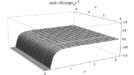
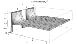
Figure 2: Low order correction to the vectorial cross section (space-like case) for different directions of the background vector: $(\theta_{v}=0,\varphi_{v}=0)$ and $(\theta_{v}=\pi/2,\varphi_{v}=0)$, respectively.

In the above result, we note the dependence of the cross section with respect to the azimuthal angle $\varphi$. For the fixed background ${\bf v}$ perpendicular to the beam collision $(\theta_{v}=\pi/2)$, this effect is maximal and it is characterized by a set of periodic sharp peaks, as illustrated in Fig.2. For the Compton scattering with the LV term in the kinetic sector a similar result was reported MSchreck .

To conclude this section, we will determine upper bounds for the products of the parameters $(gv^{\mu})$ in the cases evaluated above. Our choice to study Bhabha scattering was motivated, in addition to the questions outlined in the introduction, by practical reasons, i.e, the experimental data on precision tests for this kind of scattering in QED are readily available in Ref. MDerrick1986 . In the experiment reported in that paper, the measurements of the differential cross sections for $e^{+}e^{-}\rightarrow e^{+}e^{-}$ and $e^{+}e^{-}\rightarrow\gamma\gamma$ scatterings were evaluated at a center-of-mass energy of 29 GeV and in the polar-angular region $\left|\cos\theta\right|<0.55$. For Bhabha scattering, small deviations on the magnitude of the QED tree results may be expressed in the form:

$$\Bigg{|}\left.\left(\frac{d\sigma}{d\Omega}\right)\right/\left(\frac{d\sigma}{d\Omega}\right)_{QED}-1\Bigg{|}\approx\left(\frac{3s}{\Lambda^{2}}\right),$$ (13)

where $s=E_{cm}^{2}$ and $\Lambda$ is a small parameter representing possible experimental departures from the theoretical predictions (see Table XIV of Ref. MDerrick1986 ).

Considering the leading corrections for small ($gv^{\mu}$) in (10) and (12), we can show that the magnitude of these corrections are of order $g^{2}v^{2}s/e^{2}$, and therefore when compared with (13) may not be larger than $3s/\Lambda^{2}$. Thus, we obtain the upper bound

$$(gv^{\mu})\leq 10^{-12}(\mbox{eV})^{-1},$$ (14)

for $\Lambda=200$ GeV.

In the above calculations we provided a way to obtain bounds to LV from the analyses of the Bhabha scattering experiment using only QED interactions. The inclusion of QCD effects would improve the value of $\Lambda$ (consequently the bound) and should allow a better comparison with the results encountered for atomic clocks or torsion balances.

III Bhabha scattering: axial-like nonminimal coupling

We turn our attention now to the nonminimal coupling of chiral character, defined as

$$D_{\mu}=\partial_{\mu}+ieA_{\mu}+ig_{5}\gamma^{5}b^{\nu}F_{\mu\nu}^{\ast},$$ (15)

which was also examined in Refs. Belich2005 ; Belich2006 .

The calculation of the unpolarized cross section may be worked out similarly as in the previous section. Note that the expression for $i\mathcal{M}_{2}$ differ from (LABEL:eq:M2) just for the insertion of the $\gamma_{5}$ matrix in each matrix element, whereas for $i\mathcal{M}_{1}$ we have the mixture of the vertices:

$$i\mathcal{M}_{1} = \frac{eg_{5}b^{\nu}(p_{1}-p_{2})^{\theta}\epsilon_{\mu\nu\theta\rho}}{(p_{1}-p_{2})^{2}}\left[u(p_{2})\gamma^{\rho}u(p_{1})\overline{v}(q_{1})\gamma^{\mu}\gamma^{5}v(q_{2})\right.$$ (16)

$$\left.-\overline{u}(p_{2})\gamma^{\text{$\mu$}}\gamma^{5}u(p_{1})\overline{v}(q_{1})\gamma^{\text{$\rho$}}v(q_{2})\right]$$

$$+\frac{eg_{5}b^{\nu}(p_{1}+q_{1})^{\theta}\epsilon_{\mu\nu\theta\rho}}{(p_{1}+q_{1})^{2}}\left[\overline{u}(p_{2})\gamma^{\text{$\rho$}}v(q_{2})\overline{v}(q_{1})\gamma^{\text{$\mu$}}\gamma^{5}u(p_{1})\right.$$

$$\left.-\overline{u}(p_{2})\gamma^{\text{$\mu$}}\gamma^{5}v(q_{2})\overline{v}(q_{1})\gamma^{\text{$\rho$}}u(p_{1})\right].$$

In the high energy limit and the center of mass frame the differential cross section for the case $b^{\mu}=(b_{0},0)$ is given by

$$\frac{d\sigma}{d\Omega}_{cm} = \frac{e^{4}(\cos 2\theta+7)^{2}}{256\pi^{2}E_{cm}^{2}(\cos\theta-1)^{2}}$$ (17)

$$- \frac{b_{0}^{2}g_{5}^{2}e^{2}\sin^{4}\frac{\theta}{2}(8\cos\theta+\cos 2\theta+23)}{64\pi^{2}(\cos\theta-1)^{2}}$$

$$+ \frac{b_{0}^{4}g_{5}^{4}E_{cm}^{2}\sin^{4}\frac{\theta}{2}(-4\cos\theta+\cos 2\theta+11)}{128\pi^{2}(\cos\theta-1)^{2}}.$$

Similarly to the time-like case evaluated in the previous section, the above result contains only even terms in $(g_{5}b_{0})$. However, the asymptotic behavior is quite different and the leading-order contribution is finite in the limit $\theta\rightarrow 0$, as shown by the dotted line in Fig.1.

For the case $b^{\mu}=(0,{\bf b})$, the differential cross section becomes

$$\frac{d\sigma}{d\Omega}_{cm} = \frac{e^{4}(\cos 2\theta+7)^{2}}{256\pi^{2}E_{cm}^{2}(\cos\theta-1)^{2}}$$ (18)

$$+ \frac{e^{3}g_{5}\text{b}\sin^{2}\theta(\cos\theta+1)(\cos\theta_{5}+\cos\Psi_{5})}{16\pi^{2}E_{cm}(\cos\theta-1)^{2}}$$

$$+ \frac{e^{2}g_{5}^{2}\text{b}^{2}}{512\pi^{2}(\cos\theta-1)^{2}}\left[8(7\cos\theta-6\cos 2\theta+\cos 3\theta+14)\cos\Psi_{5}\cos\theta_{5}\right.$$

$$+ (-\cos\theta+26\cos 2\theta+\cos 3\theta-90)(\cos^{2}\theta_{5}+\cos^{2}\Psi_{5})$$

$$+ \left.6\sin^{2}\theta(-24\cos\theta+\cos 2\theta+31)\right]$$

$$+ \frac{eg_{5}^{3}\text{b}^{3}E_{cm}\sin^{2}\theta}{32\pi^{2}(\cos\theta-1)^{2}}\left[3(\cos\theta-1)+(\cos\Psi_{5}-\cos\theta_{5}){}^{2}\right](\cos\theta_{5}+\cos\Psi_{5})$$

$$+ \frac{g_{5}^{4}\text{b}^{4}E_{cm}^{2}}{1024\pi^{2}(\cos\theta-1)^{2}}\left[-4(8\cos\theta+\cos 2\theta+7)\cos^{3}\Psi_{5}\cos\theta_{5}\right.$$

$$+ 2(12\cos\theta+7\cos 2\theta+29)\cos^{2}\Psi_{5}\cos^{2}\theta_{5}$$

$$+ 4\cos\Psi_{5}\cos\theta_{5}\left(4\sin^{2}\theta(3\cos\theta+2)-(8\cos\theta+\cos 2\theta+7)\cos^{2}\theta_{5}\right)$$

$$- 2\sin^{2}\theta(3\cos\theta+7)\left(\cos 2\theta_{5}+\cos 2\Psi_{5}+2\right)$$

$$+ (4\cos\theta+\cos 2\theta+11)\cos^{4}\theta_{5}+(4\cos\theta+\cos 2\theta+11)\cos^{4}\Psi_{5}$$

$$+ \left.8\sin^{4}\frac{\theta}{2}(24\cos\theta+7\cos 2\theta+25)\right],$$

where the presence of odd-order corrections in $(g_{5}\mbox{b})$, absent in the previous vectorial cases is to be noticed. Furthermore, the effect of anisotropy in the cross-section is highlighted, as indicated in Fig. 3.

Now, an analyses similar to the previous section allows to set up an upper bound to the breaking parameter $(g_{5}b^{\mu})$. Taking into account the magnitude of the leading-order corrections for the time-like and space-like cases given respectively by $4g_{5}^{2}b_{0}^{2}s/e^{2}$ and $16g_{5}\mbox{b}\sqrt{s}/e$ and assuming that $s=29$ GeV and $\Lambda_{\pm}=200$ GeV, we find

$$g_{5}b_{0}\leq 10^{-12}(\mbox{eV})^{-1}\ \ \ \ \mbox{and}\ \ \ \ g_{5}\mbox{b}\leq 10^{-14}\mbox{(eV)}^{-1}.$$ (19)

IV Conclusion

In this paper, the implications of Lorentz symmetry breaking on Bhabha scattering have been studied. The LV background terms were introduced by nonminimal couplings between the fermion and gauge fields. We calculated the differential cross sections for the vector and axial couplings and determined upper bounds on the magnitude of the corresponding LV coefficients, by making use of accurate experimental data, available in the literature. In particular, when we consider the vector backgrounds, $v^{\mu},b^{\mu}$, as being purely spatial, the cross section acquires a nontrivial dependence on the direction of these vectors.Finally, we hope that these results may be usefull as a guide in the investigation of the Lorentz violation phenomena in high energy scattering processes.

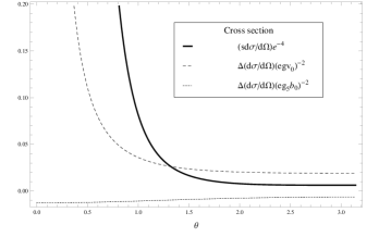
Figure 1: Angular dependence of the differential cross section for Bhabha scattering to the time-like Lorentz violation: QED prediction (solid line), vectorial (dashed line) and axial-like (dotted line) nonminimal couplings.

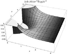
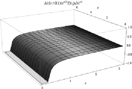
Figure 3: Low order correction to the axial-like cross section (space-like case) for different directions of the background vector: $(\theta_{5}=0,\varphi_{5}=0)$, $(\theta_{5}=\pi/2,\varphi_{5}=0)$ and $(\theta_{5}=\pi,\varphi_{5}=0)$, respectively.

References

• (1) S. M. Carroll, G. B. Field and R. Jackiw, Phys. Rev. D 41, 1231 (1990).
• (2) D. Colladay and V. A. Kostelecky , Phys. Rev. D 55, 6760 (1997).
• (3) D. Colladay and V. A. Kostelecky , Phys. Rev. D 58, 116002 (1998).
• (4) V. A. Kostelecky and R. Lehnert, Phys. Rev. D 63, 065008 (2001).
• (5) M. S. Berger and V. A. Kostelecky , Phys. Rev. D 65, 091701 (2002).
• (6) C. E. Carlson, C. D. Carone and R. F. Lebed, Phys. Lett. B 549, 337 (2002).
• (7) S. M. Carroll, J. A. Harvey, V. A. Kostelecky , C. D. Lane, and T. Okamoto, Phys. Rev. Lett. 87, 141601 (2001).
• (8) C. Csaki, J. Erlich and C. Grojean, Nucl. Phys. B 604, 312 (2001).
• (9) V. A. Kostelecky , Phys. Rev. D 69, 105009 (2004).
• (10) J. Collins, A. Perez, D. Sudarsky, L. Urrutia and H. Vucetich, Phys. Rev. Lett. 93, 191301 (2004).
• (11) B. Li, D. F. Mota and J. D. Barrow, Phys. Rev. D 77, 024032 (2008).
• (12) M. Gomes, J. R. Nascimento, A. Y. .Petrov and A. J. da Silva, Phys. Rev. D 81, 045018 (2010).
• (13) T. Mariz, J. R. Nascimento and A. Y. .Petrov, Phys. Rev. D 85, 125003 (2012).
• (14) P. R. S. Gomes and M. Gomes, Phys. Rev. D 85, 085018 (2012).
• (15) W. F. Chen and G. Kunstatter, Phys. Rev. D 62, 105029 (2000).
• (16) C. D. Carone, M. Sher and M. Vanderhaeghen, Phys. Rev. D 74, 077901 (2006).
• (17) B. Charneski, M. Gomes, T. Mariz, J. R. Nascimento and A. J. da Silva, Phys. Rev. D 81, 105025 (2010).
• (18) B. Charneski, M. Gomes, T. Mariz, J. R. Nascimento and A. J. da Silva, Phys. Rev. D 82, 105029 (2010).
• (19) D. Colladay and V. A. Kostelecky , Phys. Lett. B 511, 209 (2001).
• (20) B. Altschul, Phys. Rev. D 70, 056005 (2004).
• (21) H. Belich, T. Costa-Soares, M.M. Ferreira, Jr. and J.A. Helayel-Neto, Eur. Phys. J. C 41, 421 (2005).
• (22) H. Belich, T. Costa-Soares, M. M. Ferreira, Jr., J. A. Helayel-Neto and F. M. O. Mouchereck, Phys. Rev. D 74, 065009 (2006).
• (23) B. Charneski, M. Gomes, T. Mariz, J. R. Nascimento and A. J. da Silva, Phys. Rev. D 79, 065007 (2009).
• (24) D. Mattingly, “Modern Tests of Lorentz Invariance”, Living Rev. Relativity 8, 5 (2005).
• (25) J. M. Brown, S. J. Smullin, T. W. Kornack and M. V. Romalis, Phys. Rev. Lett. 105, 151604 (2010).
• (26) M. Schreck, “Analysis of the consistency of parity-odd nonbirefringent modified Maxwell theory,” [arXiv:1111.4182v1[hep-th]].
• (27) VENUS Collaboration, K. Abe et al., J. Phys. Soc. Jpn. 56, 3767 (1987).
• (28) TOPAZ Collaboration, I. Adachi et al., Phys. Lett. B 200, 391 (1988); AMY Collaboration, S. K. Kim et al., ibid. 223, 476 (1989).
• (29) P. B. Renton, in 17th International Symposium on Lepton-Photon Interactions, edited by Z.-P. Zheng and H.-S. Chen (World Scientific, Singapore, 1996), p. 35.
• (30) M. Derrick et al, Phys. Rev. D 34, 3286 (1986).
• (31) T. Arima et al, Phys. Rev. D 55, 19–39 (1997).
• (32) R. Mertig, M. Bohm, and A. Denner, Comput. Phys. Commun. 64, 345 (1991).
Refer to caption