Bat Algorithm for Multi-objective Optimisation

Abstract

Engineering optimization is typically multiobjective and multidisciplinary with complex constraints, and the solution of such complex problems requires efficient optimization algorithms. Recently, Xin-She Yang proposed a bat-inspired algorithm for solving nonlinear, global optimisation problems. In this paper, we extend this algorithm to solve multiobjective optimisation problems. The proposed multiobjective bat algorithm (MOBA) is first validated against a subset of test functions, and then applied to solve multiobjective design problems such as welded beam design. Simulation results suggest that the proposed algorithm works efficiently.

Keywords: Bat algorithm; cuckoo search; firefly algorithm; optimisation; multiobjective optimisation.

Reference to this paper should be made as follows:

Yang, X. S., (2011), Bat Algorithm for Multiobjective Optimization, Int. J. Bio-Inspired Computation, Vol. 3, No. 5, pp.267-274.

1 Introduction

Design optimisation in engineering often concerns multiple design objectives under complex, highly nonlinear constraints. Different objectives often conflict each other, and sometimes, truly optimal solutions do not exist, and some tradeoff and approximations are often needed. Further to this complexity, a design problem is subjected to various design constraints, limited by design codes or standards, material properties and choice of available resources and costs (Deb, 2001; Farina et al., 2004). Even for global optimisation problems with a single objective, if the design functions are highly nonlinear, global optimality is not easy to reach. Metaheuristic algorithms are very powerful in dealing with this kind of optimization, and there are many review articles and excellent textbooks (Coello, 1999; Deb, 2001; Isasi and Hernandez, 2004; Yang, 2008; Talbi, 2009; Yang, 2010c).

In contrast with single objective optimization, multiobjective problems are much difficult and complex (Coello, 1999; Floudas et al., 1999; Gong et al., 2009; Yang and Koziel, 2010). Firstly, no single unique solution is the best; instead, a set of non-dominated solutions should be found in order to get a good approximation to the true Pareto front. Secondly, even if an algorithm can find solution points on the Pareto front, there is no guarantee that multiple Pareto points will distribute along the front uniformly, often they do not. Thirdly, algorithms work well for single objective optimization usually do not directly work for multiobjective problems, unless under special circumstances such as combining multiobjectives into a single objective using some weighted sum methods. Substantial modifications are often needed. In addition to these difficulties, a further challenge is how to generate solutions with enough diversity so that new solutions can sample the search space efficiently (Talbi, 2009; Erfani and Utyuzhnikov, 2011; Yang and Koziel, 2011).

Furthermore, real-world optimization problems always involve certain degree of uncertainty or noise. For example, materials properties for a design product may vary significantly, an optimal design should be robust enough to allow such inhomogeneity and also provides good choice for decision-makers or designers. Despite these challenges, multiobjective optimization has many powerful algorithms with many successful applications (Abbass and Sarker, 2002; Banks et al., 2008; Deb, 2001, Farina et al., 2004; Konak et al., 2006; Rangaiah, 2008; Marler and Arora, 2004).

In addition, metaheuristic algorithms start to emerge as a major player for multiobjective global optimization, they often mimic the successful characteristics in nature, especially biological systems (Kennedy and Eberhart, 1995; Yang, 2005; Yang, 2010a; Yang, 2010b). Many new algorithms are emerging with many important applications (Kennedy and Eberhart, 1995; Luna et al., 2007; Osyczka and Kundu, 1995; Reyes-Sierra and Coello, 2006; Tabli, 2009; Cui and Cai, 2009; Yang, 2010c; Zhang and Li, 2007; Yang and Deb, 2010b, Yang et al., 2011). For example, a new cuckoo search algorithm was developed by Xin-She Yang and Suash Deb (2009) and more detailed studies by the same authors (Yang and Deb, 2010a) suggested that it is very efficient for solving nonlinear engineering design problems. For a recent review of popular metaheuristics, please refer to Yang (2011).

Recently, a new metaheuristic search algorithm, called bat algorithm (BA), has been developed by Xin-She Yang (2010a). Preliminary studies show that it is very promising and could outperform existing algorithms. In this paper, we will extend BA to solve multiobjective problems and formulate a multiobjective bat algorithm (MOBA). We will first validate it against a subset of multiobjective test functions. Then, we will apply it to solve design optimization problems in engineering, such as bi-objective beam design. Finally, we will discuss the unique features of the proposed algorithm as well as topics for further studies.

2 Bat Behaviour and Bat Algorithm

In order to extend the bat-inspired algorithm for single optimization to solve multiobjective problems, let us briefly review the basics of the bat algorithm for single objective optimization. Then, we will outline the basic ideas and steps of the proposed algorithm.

2.1 Echolocation of Microbats

Bats are fascinating animals. They are the only mammals with wings and they also have advanced capability of echolocation. It is estimated that there are about 996 different species which account for up to 20% of all mammal species (Altringham, 1996; Colin, 2000). Their size ranges from the tiny bumblebee bat (of about 1.5 to 2g) to the giant bats with wingspan of about 2 m and weight up to about 1 kg. Microbats typically have forearm length of about 2.2 to 11cm. Most bats uses echolocation to a certain degree; among all the species, microbats are a famous example as microbats use echolocation extensively while megabats do not (Richardson, 2008).

Microbats use a type of sonar, called, echolocation, to detect prey, avoid obstacles, and locate their roosting crevices in the dark. These bats emit a very loud sound pulse and listen for the echo that bounces back from the surrounding objects. Their pulses vary in properties and can be correlated with their hunting strategies, depending on the species. Most bats use short, frequency-modulated signals to sweep through about an octave, while others more often use constant-frequency signals for echolocation. Their signal bandwidth varies depends on the species, and often increased by using more harmonics.

Though each pulse only lasts a few thousandths of a second (up to about 8 to 10 ms), however, it has a constant frequency which is usually in the region of 25kHz to 150 kHz. The typical range of frequencies for most bat species are in the region between 25kHz and 100kHz, though some species can emit higher frequencies up to 150 kHz. Each ultrasonic burst may last typically 5 to 20 ms, and microbats emit about 10 to 20 such sound bursts every second. When hunting for prey, the rate of pulse emission can be sped up to about 200 pulses per second when they fly near their prey. Such short sound bursts imply the fantastic ability of the signal processing power of bats. In fact, studies shows the integration time of the bat ear is typically about 300 to 400 $\mu$s. As the speed of sound in air is typically $v=340$ m/s, the wavelength $\lambda$ of the ultrasonic sound bursts with a constant frequency $f$ is given by $\lambda=v/f$, which is in the range of 2mm to 14mm for the typical frequency range from 25kHz to 150 kHz. Such wavelengths are in the same order of their prey sizes.

Studies show that microbats use the time delay from the emission and detection of the echo, the time difference between their two ears, and the loudness variations of the echoes to build up three dimensional scenario of the surrounding. They can detect the distance and orientation of the target, the type of prey, and even the moving speed of the prey such as small insects (Altringham, 1996). Obviously, some bats have good eyesight, and most bats also have very sensitive smell sense. In reality, they will use all the senses as a combination to maximize the efficient detection of prey and smooth navigation. However, here we are only interested in the echolocation and the associated behaviour. Such echolocation behaviour of microbats can be formulated in such a way that it can be associated with the objective function to be optimized, and this makes it possible to formulate new optimization algorithms.

2.2 Bat Algorithm

If we idealize some of the echolocation characteristics of microbats, we can develop various bat-inspired algorithms or bat algorithms. In the basic bat algorithm developed by Xin-She Yang (2010a), the following approximate or idealized rules were used.

• All bats use echolocation to sense distance, and they also ‘know’ the difference between food/prey and background barriers in some magical way;

• Bats fly randomly with velocity ${\mbox{\boldmath$v$}}_{i}$ at position ${\mbox{\boldmath$x$}}_{i}$ with a frequency $f_{\min}$, varying wavelength $\lambda$ and loudness $A_{0}$ to search for prey. They can automatically adjust the wavelength (or frequency) of their emitted pulses and adjust the rate of pulse emission $r\in[0,1]$, depending on the proximity of their target;

• Although the loudness can vary in many ways, we assume that the loudness varies from a large (positive) $A_{0}$ to a minimum constant value $A_{\min}$.

Another obvious simplification is that no ray tracing is used in estimating the time delay and three dimensional topography. Though this might be a good feature for the application in computational geometry, however, we will not use this feature, as it is more computationally extensive in multidimensional cases.

In addition to these simplified assumptions, we also use the following approximations, for simplicity. In general the frequency $f$ in a range $[f_{\min},f_{\max}]$ corresponds to a range of wavelengths $[\lambda_{\min},\lambda_{\max}]$. For example a frequency range of [$20$kHz, $500$kHz] corresponds to a range of wavelengths from $0.7$mm to $17$mm in reality. Obviously, we can choose the ranges freely to suit different applications.

2.3 Bat Motion

For the bats in simulations, we have to define the rules how their positions ${\mbox{\boldmath$x$}}_{i}$ and velocities ${\mbox{\boldmath$v$}}_{i}$ in a $d$-dimensional search space are updated. The new solutions ${\mbox{\boldmath$x$}}_{i}^{t}$ and velocities ${\mbox{\boldmath$v$}}_{i}^{t}$ at time step $t$ are given by

$$f_{i}=f_{\min}+(f_{\max}-f_{\min})\beta,$$ (1)

$${\mbox{\boldmath$v$}}_{i}^{t+1}={\mbox{\boldmath$v$}}_{i}^{t}+({\mbox{\boldmath$x$}}_{i}^{t}-{\mbox{\boldmath$x$}}_{*})f_{i},$$ (2)

$${\mbox{\boldmath$x$}}_{i}^{t+1}={\mbox{\boldmath$x$}}_{i}^{t}+{\mbox{\boldmath$v$}}_{i}^{t},$$ (3)

where $\beta\in[0,1]$ is a random vector drawn from a uniform distribution. Here ${\mbox{\boldmath$x$}}_{*}$ is the current global best location (solution) which is located after comparing all the solutions among all the $n$ bats at each iteration $t$. As the product $\lambda_{i}f_{i}$ is the velocity increment, we can use $f_{i}$ (or $\lambda_{i}$ ) to adjust the velocity change while fixing the other factor $\lambda_{i}$ (or $f_{i}$), depending on the type of the problem of interest. In our implementation, we will use $f_{\min}=0$ and $f_{\max}=O(1)$, depending on the domain size of the problem of interest. Initially, each bat is randomly assigned a frequency which is drawn uniformly from $[f_{\min},f_{\max}]$.

For the local search part, once a solution is selected among the current best solutions, a new solution for each bat is generated locally using random walk

$${\mbox{\boldmath$x$}}_{\rm new}={\mbox{\boldmath$x$}}_{\rm old}+{\mbox{\boldmath$\epsilon$}}\;A^{t},$$ (4)

where $\epsilon$ is a random number vector drawn from $[-1,1]$, while $A^{t}=<\!\!A_{i}^{t}\!>$ is the average loudness of all the bats at this time step.

The update of the velocities and positions of bats have some similarity to the procedure in the standard particle swarm optimization, as $f_{i}$ essentially controls the pace and range of the movement of the swarming particles. To a degree, BA can be considered as a balanced combination of the standard particle swarm optimization and the intensive local search controlled by the loudness and pulse rate.

2.4 Loudness and Pulse Emission

Furthermore, the loudness $A_{i}$ and the rate $r_{i}$ of pulse emission have to be updated accordingly as the iterations proceed. As the loudness usually decreases once a bat has found its prey, while the rate of pulse emission increases, the loudness can be chosen as any value of convenience. For example, we can use $A_{0}=100$ and $A_{\min}=1$. For simplicity, we can also use $A_{0}=1$ and $A_{\min}=0$, assuming $A_{\min}=0$ means that a bat has just found the prey and temporarily stop emitting any sound. Now we have

$$A_{i}^{t+1}=\alpha A_{i}^{t},\;\;\;\;\;r_{i}^{t}=r_{i}^{0}[1-\exp(-\gamma t)],$$ (5)

where $\alpha$ and $\gamma$ are constants. In fact, $\alpha$ is similar to the cooling factor of a cooling schedule in the simulated annealing (Kirkpatrick et al., 1983). For any $0<\alpha<1$ and $\gamma>0$, we have

$$A_{i}^{t}\rightarrow 0,\;\;\;r_{i}^{t}\rightarrow r_{i}^{0},\;\;\textrm{as}\;\;t\rightarrow\infty.$$ (6)

In the simplest case, we can use $\alpha=\gamma$, and we have used $\alpha=\gamma=0.9$ in our simulations.

Preliminary studies by Yang (2010a) suggested that bat algorithm is very promising for solving nonlinear global optimization problems. Now we extend it to solve multiobjective optimization problems.

3 Multiobjective Bat Algorithm

Multiobjective optimization problems are more complicated than single objective optimization, and we have to find and/or approximate the optimality fronts. In addition, algorithms have to be modified to accommodate multiobjectives properly.

3.1 Pareto Optimality

A solution vector ${\mbox{\boldmath$u$}}=(u_{1},..,u_{n})^{T}\in{\cal F}$, is said to dominate another vector ${\mbox{\boldmath$v$}}=(v_{1},...,v_{n})^{T}$ if and only if $u_{i}\leq v_{i}$ for $\forall i\in\{1,...,n\}$ and $\exists i\in\{1,...,n\}:u_{i}<v_{i}.$ In other words, no component of $u$ is larger than the corresponding component of $v$, and at least one component is smaller. Similarly, we can define another dominance relationship $\preceq$ by

$${\mbox{\boldmath$u$}}\preceq{\mbox{\boldmath$v$}}\Longleftrightarrow{\mbox{\boldmath$u$}}\prec{\mbox{\boldmath$v$}}\vee{\mbox{\boldmath$u$}}={\mbox{\boldmath$v$}}.$$ (7)

It is worth pointing out that for maximization problems, the dominance can be defined by replacing $\prec$ with $\succ$. Therefore, a point ${\mbox{\boldmath$x$}}_{*}\in{\cal F}$ is called a non-dominated solution if no solution can be found that dominates it (Coello, 1999).

The Pareto front $PF$ of a multiobjective can be defined as the set of non-dominated solutions so that

$$PF=\{{\mbox{\boldmath$s$}}\in{\cal S}\Big{|}\exists/\;{\mbox{\boldmath$s^{\prime}$}}\in{\cal S}:{\mbox{\boldmath$s^{\prime}$}}\prec{\mbox{\boldmath$s$}}\},$$ (8)

or in term of the Pareto optimal set in the search space

$$PF^{*}=\{{\mbox{\boldmath$x$}}\in{\cal F}\Big{|}\exists/\;{\mbox{\boldmath$x^{\prime}$}}\in{\cal F}:{\mbox{\boldmath$f(x^{\prime})$}}\prec{\mbox{\boldmath$f(x)$}}\},$$ (9)

where ${\mbox{\boldmath$f$}}=(f_{1},...,f_{K})^{T}$. To obtain a good approximation to Pareto front, a diverse range of solutions should be generated using efficient techniques (Gujarathi and Babu, 2009; Konak et al., 2006).

3.2 MOBA Algorithm

Based on these approximations and idealization, the basic steps of the multiobjective bat algorithm (MOBA) can be summarized as the pseudo code shown in Fig. 1.

  Objective functions $f_{1}({\mbox{\boldmath$x$}}),...,f_{K}({\mbox{\boldmath$x$}})$, ${\mbox{\boldmath$x$}}=(x_{1},...,x_{d})^{T}$

Initialize the bat population ${\mbox{\boldmath$x$}}_{i}\;(i=1,2,...,n)$ and ${\mbox{\boldmath$v$}}_{i}$
for $j=1$ to $N$ (points on Pareto fronts)
 Generate $K$ weights $w_{k}\geq 0$ so that $\sum_{k=1}^{K}w_{k}=1$
 Form a single objective $f=\sum_{k=1}^{K}w_{k}f_{k}$
 while ($t<$Max number of iterations)
  Generate new solutions and update by (1) to (3)
  if (rand $>r_{i}$)
   Random walk around a selected best solution
  end if
  Generate a new solution by flying randomly
  if (rand $<A_{i}\;\;\&\;\;f({\mbox{\boldmath$x$}}_{i})<f({\mbox{\boldmath$x$}}_{*})$)
   Accept the new solutions,
   and increase $r_{i}$ & reduce $A_{i}$
  end if
  Rank the bats and find the current best ${\mbox{\boldmath$x$}}_{*}$
 end while
 Record ${\mbox{\boldmath$x$}}_{*}$ as a non-dominated solution
end
Postprocess results and visualization  

Figure 1: Multiobjective bat algorithm (MOBA).

For simplicity here, we use a weighted sum to combine all objectives $f_{k}$ into a single objective

$$f=\sum_{k=1}^{K}w_{k}f_{k},\quad\sum_{k=1}^{K}w_{k}=1.$$ (10)

As the weights are generated randomly from a uniform distribution, it is possible to vary the weights with sufficient diversity so that the Pareto front can be approximated correctly.

In our simulations, we have carried out parametric studies, and we have used $\alpha=\gamma=0.9$ for all simulations. The choice of parameters requires some experimenting. Initially, each bat should have different values of loudness and pulse emission rate, and this can be achieved by randomization. For example, the initial loudness $A_{i}^{0}$ can typically be $[1,2]$, while the initial emission rate $r_{i}^{0}$ can be around zero, or any value $r_{i}^{0}\in[0,1]$ if using (5). Their loudness and emission rates will be updated only if the new solutions are improved, which means that these bats are moving towards the optimal solution.

4 Numerical Results

4.1 Parametric Studies

The proposed multiobjective bat algorithm (MOBA) is implemented in Matlab, and computing time is within a few seconds to less than a minute, depending on the problem of interest. We have tested it using a different range of parameters such as population size ($n$), loudness reduction $\alpha$, and pulse reduction rate $\gamma$. By varying $n=5,10,15,20,30,50$ to $50,100,150$, $200,250,300,400,500$, $\alpha=0.5,0.6,0.7$, $0.8,0.9,0.95,1$ and $\gamma=0.5,0.6,0.7$, $0.8,0.9,0.95,1,0$, we found that the best parameters for most applications are: $n=25$ to $50$, $\alpha=0.7$ to $0.9$ and $\gamma=0.7$ to $0.9$.

The stopping criterion can be defined in many ways. We can either use a given tolerance or a fixed number of iterations. From the implementation point of view, a fixed number of iterations is not only easy to implement, but also suitable to compare the closeness of Pareto front of different functions. So we have set the fixed number iterations as 5000, which is sufficient for most problems. If necessary, we can also increase it to a larger number.

In order to generate more optimal points on the Pareto front, we can do it in two ways: increase the population size $n$ or run the program a few more times. Through simulations, we found that to increase of $n$ typically leads to a longer computing time than to re-run the program a few times. This may be due to the fact that manipulations of large matrices or longer vectors usually take longer. Another possibility is that simple restart can increase the diversity of solutions than more intensive search for longer iterations. So to generate 200 points using a population size $n=50$ requires to run the program 4 times, which is easily done within a few minutes. Therefore, in all our simulations, we will use the fixed parameters: $n=50$, $\alpha=\gamma=0.9$.

4.2 Multiobjective Test Functions

There are many different test functions for multobjective optimization (Schaffer, 1985; Zhang et al., 2003; Zhang et al, 2009; Zitzler and Thiele, 1999; Zitzler et al., 2000), but a subset of a few widely used functions provides a wide range of diverse properties in terms Pareto front and Pareto optimal set. To validate the proposed MOBA, we have selected a subset of these functions with convex, non-convex and discontinuous Pareto fronts. We also include functions with more complex Pareto sets. To be more specific in this paper, we have tested the following four functions:

ZDT1 function with a convex front (Zitzler and Thiele 1999; Zitzler et al. 2000)

$$f_{1}(x)=x_{1},\quad f_{2}(x)=g(1-\sqrt{f_{1}/g}),$$

$$g=1+\frac{9\sum_{i=2}^{d}x_{i}}{d-1},\quad x_{i}\in[0,1],\;i=1,...,30,$$ (11)

where $d$ is the number of dimensions. The Pareto-optimality is reached when $g=1$.

ZDT2 function with a non-convex front

$$f_{1}(x)=x_{1},\quad f_{2}(x)=g(1-\frac{f_{1}}{g})^{2},$$

ZDT3 function with a discontinuous front

$$f_{1}(x)=x_{1},\quad f_{2}(x)=g\Big{[}1-\sqrt{\frac{f_{1}}{g}}-\frac{f_{1}}{g}\sin(10\pi f_{1})\Big{]},$$

where $g$ in functions ZDT2 and ZDT3 is the same as in function ZDT1. In the ZDT3 function, $f_{1}$ varies from $0$ to $0.852$ and $f_{2}$ from $-0.773$ to $1$.

LZ4 function (Li and Zhang, 2009; Zhang and Li, 2007)

$$f_{1}=x_{1}+\frac{2}{|J_{1}|}\sum_{j\in J_{1}}h(u_{j})$$

$$f_{2}=1-x_{1}^{2}+\frac{2}{|J_{2}|}\sum_{j\in J_{2}}h(u_{j}),$$ (12)

where $J_{1}=\{j|j$ is odd and $2\leq j\leq d\}$ and $J_{2}=\{j|j$ is even and $2\leq j\leq d\}$.

$$u_{j}=x_{j}-\sin(6\pi x_{1}+\frac{j\pi}{d}),$$

$$x_{1}\in[0,1],\;x_{j}\in[-2,2],\;j=2,...,d,$$

and

$$h(v)=\frac{|v|}{1+e^{2|v|}}.$$ (13)

This function has a Pareto front $f_{2}=1-f_{1}^{2}$ for $0\leq f_{1}\leq 1$ with a Pareto set

$$x_{j}=\sin(6\pi x_{1}+\frac{j\pi}{d}),\quad j=2,3,...,d,\quad x_{1}\in[0,1].$$ (14)

After generating 200 Pareto points by MOBA, the Pareto front generated by MOBA is compared with the true front $f_{2}=1-\sqrt{f_{1}}$ of ZDT1 (see Fig. 2). In all the rest of the figures, the vertical axis is for $f_{2}$ while the horizontal axis is for $f_{1}$.

Table 1: Summary of results.

Functions	Errort=2000	Errort=5000
ZDT1	3.7E-4	4.5E-17
ZDT2	2.4E-4	3.2E-19
ZDT3	5.2E-5	1.7E-15
LZ4	2.9E-4	1.2E-16

Let us define the distance or error between the estimate Pareto front $PF^{e}$ to its correspond true front $PF^{t}$ as

$$E_{f}=||PF^{e}-PF^{t}||^{2}=\sum_{j=1}^{N}(PF_{j}^{e}-PF_{t})^{2},$$ (15)

where $N$ is the number of points. The convergence property can be viewed by following the iterations. Figs. 3 and 4 show the exponential-like decrease of $E_{f}$ as the iterations proceed. The least-square distance from the estimated front to the true front of ZDT1 for the first 1000 iterations (Fig. 3) and the logarithmic scale for 5000 iterations (Fig. 4).

We can see clearly that our MOBA algorithm indeed converges almost exponentially. The results for all the functions are summarized in Table 1. We can see that exponential convergence can be achieved in all cases.

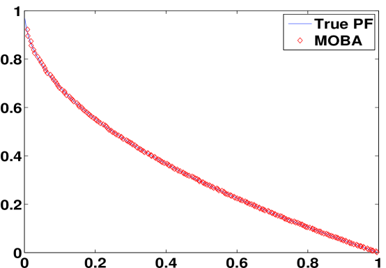
Figure 2: Estimated front and true front for ZDT1.

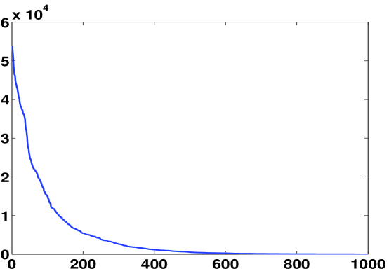
Figure 3: Convergence of the MOBA.

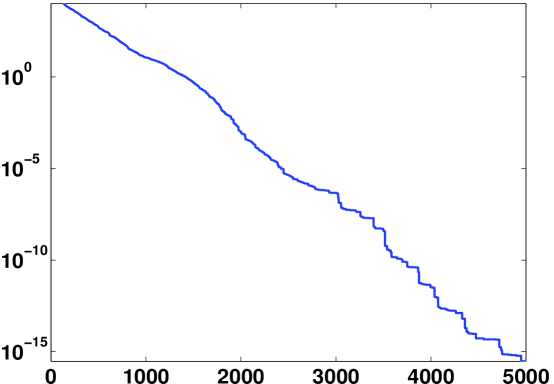
Figure 4: Exponential convergence of the MOBA.

5 Engineering Optimization

Design optimization, especially design of structures, has many applications in engineering and industry. As a result, there are many different benchmarks with detailed studies in the literature (Pham and Ghanbarzadeh, 2007; Ray and Liew, 2002; Rangaiah, 2008). Among the widely used benchmarks, the welded beam design is a well-known design problem. In the rest of this paper, we will solve this design benchmark using MOBA.

Multiobjective design of a welded beam is a classical benchmark which has been solved by many researchers (Deb, 1999; Gong et al., 2009; Ray and Liew, 2002). The problem has four design variables: the width $w$ and length $L$ of the welded area, the depth $d$ and thickness $h$ of the main beam. The objectives are to minimize both the overall fabrication cost and the end deflection $\delta$.

The problem can be written as

$$\textrm{minimise }\;f_{1}({\mbox{\boldmath$x$}})=1.10471w^{2}L+0.04811dh(14.0+L),$$

$$\textrm{ minimize }\;f_{2}=\delta,$$ (16)

subject to

$$\begin{array}[]{lll}g_{1}({\mbox{\boldmath$x$}})=w-h\leq 0,\vspace{2pt}\\ \vspace{3pt}g_{2}({\mbox{\boldmath$x$}})=\delta({\mbox{\boldmath$x$}})-0.25\leq 0,\\ \vspace{3pt}g_{3}({\mbox{\boldmath$x$}})=\tau({\mbox{\boldmath$x$}})-13,600\leq 0,\\ \vspace{3pt}g_{4}({\mbox{\boldmath$x$}})=\sigma({\mbox{\boldmath$x$}})-30,000\leq 0,\\ \vspace{3pt}g_{5}({\mbox{\boldmath$x$}})=0.10471w^{2}+0.04811hd(14+L)-5.0\leq 0,\\ \vspace{3pt}g_{6}({\mbox{\boldmath$x$}})=0.125-w\leq 0,\\ \vspace{3pt}g_{7}({\mbox{\boldmath$x$}})=6000-P({\mbox{\boldmath$x$}})\leq 0,\end{array}$$ (17)

where

$$\begin{array}[]{ll}\sigma({\mbox{\boldmath$x$}})=\frac{504,000}{hd^{2}},&Q=6000(14+\frac{L}{2}),\\ \\ D=\frac{1}{2}\sqrt{L^{2}+(w+d)^{2}},&J=\sqrt{2}\;wL[\frac{L^{2}}{6}+\frac{(w+d)^{2}}{2}],\\ \\ \delta=\frac{65,856}{30,000hd^{3}},&\beta=\frac{QD}{J},\\ \\ \alpha=\frac{6000}{\sqrt{2}wL},&\tau({\mbox{\boldmath$x$}})=\sqrt{\alpha^{2}+\frac{\alpha\beta L}{D}+\beta^{2}},\end{array}$$ (18)

$$P=0.61423\times 10^{6}\;\frac{dh^{3}}{6}(1-\frac{d\sqrt{30/48}}{28}).$$ (19)

The simple limits or bounds are $0.1\leq L,d\leq 10$ and $0.125\leq w,h\leq 2.0$.

By using the MOBA, we have solved this design problem. The approximate Pareto front generated by the 50 non-dominated solutions after 1000 iterations are shown in Fig. 5. This is consistent with the results obtained by others (Ray and Liew, 2002; Pham and Ghanbarzadeh, 2007). In addition, the results are more smooth with fewer iterations.

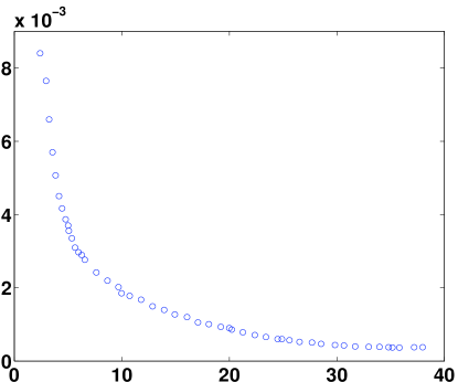
Figure 5: Pareto front for the bi-objective beam design.

The simulations for these benchmarks and functions suggest that MOBA is a very efficient algorithm for multiobjective optimization. It can deal with highly nonlinear problems with complex constraints and diverse Pareto optimal sets.

6 Conclusions

Multiobjective optimization problems are typically very difficult to solve. In this paper, we have successfully formulated a new algorithm for multiobjective optimization, namely, multiobjective bat algorithm, based on the recently developed bat algorithm. The proposed MOBA has been tested against a subset of well-chosen test functions, and then been applied to solve design optimization benchmarks in structural engineering. Results suggest that MOBA is an efficient multiojective optimizer.

Additional tests and comparison of the proposed are highly needed. In the future work, we will focus on the parametric studies for a wider range of test problems, including discrete and mixed type of optimization problems. We will try to test the diversity of the Pareto front it can generate so as to identify the ways to improve this algorithm to suit a diverse range of problems. There are a few efficient techniques to generate diverse Pareto fronts (Erfani and Utyuzhnikov 2011), and some combination with these techniques may improve MOBA even further.

Further research can also emphasize the performance comparison of this algorithm with other popular methods for multiobjective optimization. In addition, hybridization with other algorithms may also prove to be fruitful.

References

- [1]
- [2] bbass H. A. and Sarker R., (2002). The Pareto diffential evolution algorithm, Int. J. Artificial Intelligence Tools, 11(4), 531-552 (2002).
- [3] ltringham, J. D.: Bats: Biology and Behaviour, Oxford Univesity Press, (1996).
- [4] anks A., Vincent J. and Anyakoha C., (2008). A review of particle swarm optimization. Part II: hydridisation, combinatorial, multicriteria and constrained optimization, and indicative applications, Natural Computing, 109-124 (2008).
- [5] oello C. A. C., (1999). An updated survey of evolutionary multiobjective optimization techniques: state of the art and future trends, in: Proc. of 1999 Congress on Evolutionary Computation, CEC99, DOI 10.1109/CEC.1999.781901
- [6] olin, T.: The Varienty of Life. Oxford University Press, (2000).
- [7] ui Z. H., and Cai X. J. (2009) ‘Integral particle swarm optimisation with dispersed accelerator information’, Fundam. Inform., Vol. 95, 427–447.
- [8] eb K., (1999). Evolutionary algorithms for multi-criterion optimization in engieering design, in: Evolutionary Aglorithms in Engineering and Computer Science, Wiley, pp. 135-161.
- [9] eb K., (2001). Multi-Objective optimization using evolutionary algorithms, John Wiley & Sons, New York.
- [10] rfani T. and Utyuzhnikov S., (2011). Directed search domain: a method for even generation of Pareto frontier in multiobjective optimization, Engineering Optimization, (in press)
- [11] arina M., Deb K. and Amota P., (2004). Dynamic multiobjective optimization problems: test cases, approximations, and applications, IEEE Trans. Evol. Comp., 8, 425-442.
- [12] loudas C. A., Pardalos P. M., Adjiman C. S., Esposito W. R., Gumus Z. H., Harding S. T., Klepeis J. L., Meyer C. A., Scheiger C. A., (1999). Handbook of Test Problems in Local and Global Optimization, Springer.
- [13] ong W. Y., Cai Z. H., Zhu L., An effective multiobjective differential evolution algorithm for engineering design, Struct. Multidisc. Optimization, 38, 137-157 (2009).
- [14] ujarathi A. M. and Babu B. V., (2009). Improved Strategies of Multi-objective Differential Evolution (MODE) for Multi-objective Optimization, in: Proc. of 4th Indian International Conference on Artificial Intelligence (IICAI-09), December 16-18, 2009.
- [15] sasi P., and Hernandez J. C., (2004). Introduction to the Applications of Evolutionary Computation in Computer Security, Computational Intelligence, 20(3), 445-449
- [16] ennedy J. and Eberhart R. C., (1995). Particle swarm optimization. Proc. of IEEE International Conference on Neural Networks, Piscataway, NJ. pp. 1942-1948.
- [17] irkpatrick S., Gellat C. D. and Vecchi M. P., Optimization by simulated annealing, Science, 220, 670-680 (1983).
- [18] onak A., Coit D. W. and Smith A. E., (2006). Multiobjective optimization using genetic algorithms: a tutorial, Reliability Engineering and System Safety, 91, 992-1007.
- [19] i H. and Zhang Q. F., (2009). Multiobjective optimization problems with complicated Paroto sets, MOEA/D and NSGA-II, IEEE Trans. Evol. Comput., 13, 284-302.
- [20] una F., Alba E., Nebro A. J. and Pedraza S., (2007). Evolutionary algorithms for real-world instances of the automatic frequency planning problem in GSM networks, Proc. 7th Euro. Conf. Evol. Comput. Combin. Optim. (EvoCOP’07), Springer-Verlag, (2007).
- [21] arler R. T. and Arora J. S., (2004). Survey of multi-objective optimization methods for engineering, Struct. Multidisc. Optim., 26, 369-395.
- [22] syczka A. and Kundu S., (1995). A genetic algorithm-based multicriteria optimization method, Proc. 1st World Congr. Struct. Multidisc. Optim., Elsevier Sciencce, pp. 909-914.
- [23] ham D. T. and Ghanbarzadeh A., (2007). Multi-Objective Optimisation using the Bees Algorithm, in: 3rd International Virtual Conference on Intelligent Production Machines and Systems (IPROMS 2007): Whittles, Dunbeath, Scotland, 2007
- [24] angaiah G., Multi-objective Optimization: Techniques and Applications in Chemical Engineering, World Scientific Publishing, (2008).
- [25] ay L. and Liew K. M., (2002). A swarm metaphor for multiobjective design optimization, Eng. Opt., 34(2), 141-153.
- [26] eyes-Sierra M. and Coello C. A. C., (2006). Multi-objective particle swarm optimizers: A survey of the state-of-the-art, Int. J. Comput. Intelligence Res., 2(3), 287-308.
- [27] ichardson, P.: Bats. Natural History Museum, London, (2008). Also, Richardson, P.: The secrete life of bats. http://www.nhm.ac.uk
- [28] chaffer J.D., (1985). Multiple objective optimization with vector evaluated genetic algorithms, in: Proc. 1st Int. Conf. Genetic Aglorithms, pp. 93-100.
- [29] albi E.-G., (2009). Metaheuristics: From Design to Implementation, John Wiley and Sons, 624 pp.
- [30] ang X. S., (2005). Engineering optimization via nature-inspired virtual bee algorithms, in: Artificial Intelligence and Knowledge Engineering Applications: A Bioinspired Approach, Lecture Notes in Computer Science, 3562, pp. 317-323.
- [31] ang X. S., (2008) Introduction to Computational Mathematics, World Scientific Publishing.
- [32] ang X. S. and Deb S. (2009) Cuckoo search via Lévy flights, in: Proc. of World Congress on Nature & Biologically Inspired Computing (NaBic 2009), IEEE Publications, USA, pp. 210-214.
- [33] ang, X. S. (2010a). A new metaheuristic bat-inspired algorithm, in: Nature Inspired Cooperative Strategies for Optimization (NICSO 2010) (Eds. J. R. Gonzalez et al.), Springer, SCI Vol. 284, 65-74.
- [34] ang X. S., (2010b). Nature-Inspired Metaheuristic Algorithms, 2nd Edition, Luniver Press, UK.
- [35] ang X. S., (2010c). Engineering Optimisation: An Introduction with Metaheuristic Applications, John Wiley and Sons.
- [36] ang X. S. and Deb S. (2010a) Engineering optimisation by cuckoo search, Int. J. Math. Modelling & Num. Optimisation, Vol. 1, 330-343.
- [37] ang X. S. and Deb S., (2010b). Eagle strategy using Lévy walk and firefly algorithms for stochastic optimization, in: Nature-Inspiref Cooperative Strategies for Optimization (NICSO 2010), Studies in Computational Intelligence, 284, pp. 101-111.
- [38] ang X. S., Deb S., and Fong S., (2011). Accelerated particle swarm optimization and support vector machine for business optimization and applications, in: NDT 2011, Communications in Computer and Information Science, 136, pp. 53-66.
- [39] ang X. S., Review of metaheuristics and generalized evolutionary walk algorithm, Int. J. Bio-Inspired Compuation, 3(2), 77-84 (2011).
- [40] ang X. S. and Koziel S., Computational optimization, modelling and simulation – a paradigm shift, Procedia in Computer Science, 1, 1291-1294 (2010).
- [41] ang X. S. and Koziel S., Computational Optimization and Applications in Engineering and Industry, Springer, (2011).
- [42] hang L. B., Zhou C. G., Liu X. H., Ma Z. Q., Liang Y. C. (2003), Solving multi objective optimization problems using particle swarm optimization. In: Proceedings of the 2003 congress on evolutionary computation (CEC 2003), vol 4. IEEE Press, Canberra, Australia, pp. 2400 2405, December 2003
- [43] hang Q. F., Zhou A. M., Zhao S. Z., Suganthan P. N., Liu W., Tiwari S., (2009). Multiobjective optimization test instances for the CEC 2009 special session and competition, Technical Report CES-487, University of Essex, Nanyang Technological University, and Clemson University, April 2009.
- [44] hang Q. F. and Li H., (2007). MOEA/D: a multiobjective evolutionary algorithm based on decomposition, IEEE Trans. Evol. Comput., 11, 712-731 (2007).
- [45] itzler E. and Thiele L., (1999). Multiobjective evolutonary algorithms: A comparative case study and the strength pareto approach, IEEE Evol. Comp., 3, 257-271.
- [46] itzler E., Deb K., and Thiele L., (2000). Comparison of multiobjective evolutionary algorithms: Empirical results, Evol. Comput., 8, pp. 173 195