The dynamics of inner dead-zone boundaries in protoplanetary disks

Abstract

In protoplanetary disks, the inner radial boundary between the MRI turbulent (‘active’) and MRI quiescent (‘dead’) zones plays an important role in models of the disk evolution and in some planet formation scenarios. In reality, this boundary is not well-defined: thermal heating from the star in a passive disk yields a transition radius close to the star ($<0.1$ au), whereas if the disk is already MRI active, it can self-consistently maintain the requisite temperatures out to a transition radius of roughly 1 au. Moreover, the interface may not be static; it may be highly fluctuating or else unstable. In this paper, we study a reduced model of the dynamics of the active/dead zone interface that mimics several important aspects of a real disk system. We find that MRI-transition fronts propagate inward (a ‘dead front’ suppressing the MRI) if they are initially at the larger transition radius, or propagate outward (an ‘active front’ igniting the MRI) if starting from the smaller transition radius. In both cases, the front stalls at a well-defined intermediate radius, where it remains in a quasi-static equilibrium. We propose that it is this new, intermediate stalling radius that functions as the true boundary between the active and dead zones in protoplanetary disks. These dynamics are likely implicated in observations of variable accretion, such as FU Ori outbursts, as well as in those planet formation theories that require the accumulation of solid material at the dead/active interface.

1 Introduction

Protostellar disks, unlike the classic archetypes associated with dwarf novae and X-ray binaries, are enormous, cold, and poorly ionised. In fact, significant regions within these disks are so weakly coupled to the magnetic field that MRI turbulence fails to develop (Balbus and Hawley 1991, Blaes and Balbus 1994, Gammie 1996, Igea and Glassgold 1999, Sano et al. 2000). Current models of protoplanetary disk structure consist of a turbulent envelope of plasma (the ‘active zone’) encasing an extensive body of quiescent gas (the ‘dead zone’) (Gammie 1996, Armitage 2011). In particular, these models posit a critical inner radius within which the disk is fully turbulent, and beyond which the disk exhibits a characteristic layered structure for some range of radii.

In general, it is unlikely that such a configuration supports steady accretion onto the protostar (Gammie 1996, but see also Terquem 2008). In fact, observations of YSOs show a rich assortment of time-variable accretion, the most striking of which are the outbursts associated with FU Ori and EX Lupi disks (Hartmann and Kenyon 1996, Herbig 2008). In addition, measurements of disk outflows reveal quasi-periodic variability on the order of years to hundreds of years that may arise from fluctuating accretion in the inner disk, precisely at those radii where we might expect the inner dead/active zone boundary (Lopez-Martin et al. 2003, Raga et al. 2011, Agra-Amboage et al. 2011).

Theoretical models that describe FU Ori behaviour attribute an important role to the dynamics of this critical inner interface. In particular, many models interpret outburst events as the abrupt ignition of the dead-zone in turbulence, and hence the temporary dissolution of the critical boundary (Gammie 1996, Armitage et al. 2002, Zhu et al. 2009, 2010). On the other hand, local numerical simulations of the MRI near marginality — the relevant regime at the interface — also exhibit strong variability in the form of violent intermittency (channel flows) (Miller and Stone 2000, Sano and Inutsuka 2001, Latter et al. 2009, 2010) and oscillatory behaviour (Simon et al. 2011). The simulations demonstrate that the MRI will not smoothly ‘die away’ as one crosses into the dead zone through the transition layer. Despite these considerations, the interface is assumed to be effectively static in a number of planet formation scenarios (Varniére and Tagger 2006, Kretke et al. 2009, Dzyurkevich et al. 2010). The fate of these theories is unclear if indeed the interface is the site of the regular and violent dynamics suggested by observations and simulations.

Our paper is concerned with the location, radial morphology, and dynamics of this important disk feature. We concentrate on an under-appreciated ambiguity in the location of the interface, one that can potentially have consequences for the observations and processes discussed above. Gas at the midplane is thermally ionised by the central star to sufficient levels for the MRI to operate, but only out to a critical radius $R_{c}^{\text{rad}}$ very close to the star ($<0.1$ au). Beyond this radius lies a broader region in which stellar radiation fails but ionisation by turbulent heating succeeds. However, this requires there to be enough ionisation in the first place to get the MRI turbulence initiated. If the gas in this region starts off cold and poorly ionised it will remain so; conversely, if it begins hot and turbulent it can sustain this turbulent state via its own waste heat. In other words, the gas is ‘bistable’: it can fall into one of two quasi-steady states, active or dead. Finally, beyond a second critical radius $R_{c}^{\text{turb}}$ ($\sim 1$ au) neither stellar nor turbulent heating is sufficient and the disk requires non-thermal sources to ionise the midplane. Usually this second critical radius is taken to be the actual inner edge of the dead zone. This need not be the case. The interface could in principle fall within the bistable region at smaller radii, and it need not be well-defined nor time-steady.

In order to study this physics we develop a reduced MHD model that describes the interpenetration of the turbulence and the thermodynamics. It generalises the evolution equations of Lesaffre et al. (2009), which couple the thermal energy with the turbulent energy, and installs a spatial (radial) degree of freedom. The gross disk dynamics are hence represented by two coupled reaction-diffusion equations. The main prediction of this model is that the dead/active interface, though well-defined, is not always stationary. It tends to travel radially inward or outward depending on conditions at its present radial location. Ultimately the interface comes to a halt at a special radius, some 65% of the second critical radius $R_{c}^{\text{turb}}$. Moreover the interface is relatively broad, with the temperature transition layer extending over roughly 1 au. Numerical simulations should be able to check these predictions, while also assessing the prevalence and importance of turbulent intermittency.

The organisation of this paper as follows. In Section 2, we develop the concept that gas in the inner zone of protostellar disks is bistable. In Section 3, we present a reduced model that displays the fundamental behaviour of the dynamical system. This behaviour is more fully elucidated in Sections 4 and 5, in which the model is explored and its predictions presented. Next, the theory is applied, in Section 6, to what we argue is a more realistic model for the inner region of protostellar disks. Finally, in Section 7 we summarize our findings and draw our conclusions.

2 The inner regions of a protoplanetary disk: a bistable system

This section develops the idea that gas in the inner disk can fall into one of two states: a hot turbulent state, and a cooler quiescent state. We obtain a criterion for the instigation of MRI turbulence and show at which radii in the disk this is satisfied if we consider (a) radiation from the central star, in the absence of turbulence, and (b) thermal ionisation from turbulent dissipation, in the absence of stellar radiation. The latter radius can be significantly greater than the former, opening up a liminal region whose properties we discuss. For clarity, we focus on gas at the midplane only, but our calculations can be generalised to include the vertical structure of the disk.

2.1 Criterion for the onset of MRI

The MRI only functions when there is adequate coupling between the gas and the magnetic field. An estimate of the critical ionisation fraction necessary for this coupling can be obtained within the bounds of resistive MHD. Hall effects are of comparable importance in certain regions of the disk (Wardle 1999, Balbus and Terquem 2001, Wardle and Salmeron 2012), but for the sake of clarity they will be neglected; we expect no qualitative change in our calculation.

The shortest MRI-active mode works on the resistive scale: $l_{\eta}=\eta/v_{A}$, where $\eta$ is the Ohmic resistivity and $v_{A}$ is the Alfvén speed. This lengthscale cannot be larger than the disk scale height $H$. So we have marginal MRI when $l_{\eta}=H$ which gives

$$\mathcal{L}\equiv v_{A}H/\eta=1,$$ (1)

where $\mathcal{L}$ is the Lundquist number. To turn this into a critical ionisation fraction we take $H\approx 0.1R$ and the following expression for resistivity

$$\eta=234\,x_{e}^{-1}T^{1/2}\,\text{cm}^{2}\,\text{s}^{-1},$$ (2)

where $x_{e}$ is electron fraction and $T$ is temperature (Blaes and Balbus 1994). Combining these equations gives the critical ionisation level:

$$(x_{e})_{\text{crit}}=1.89\times 10^{-14}\,\beta^{1/2}\,R_{\text{AU}}^{-1},$$ (3)

where $\beta$ is the plasma beta and $R_{\text{AU}}$ is disk radius in units of au (see also Balbus 2011). At 1 au and $\beta=10^{2}-10^{3}$ we have the fiducial limit of $x_{e}\sim 10^{-13}$.

Ionisation in a protoplanetary disk can be caused by non-thermal sources, such as cosmic rays, stellar X-rays, radionuclides, and energetic stellar protons (Stepinski 1992, Gammie 1996, Igea and Glassgold 1999, Turner and Drake 2009), in addition to direct heating from either the central star or turbulent dissipation. Each source gives rise to a spatial ionisation structure in the disk. In the case of thermal ionisation, this structure follows directly from the disk’s temperature profile, and hence we can associate a critical temperature $T_{\text{MRI}}$ with the critical ionisation fraction $(x_{e})_{\text{crit}}$. The critical temperature may be computed with the aid of an appropriate form of Saha’s equation, noting that the ionisation is controlled by the low ionisation-potential alkali metals (Pneuman and Mitchell 1965, Umebayashi and Nakano 1988). A straightforward calculation (e.g. Stone et al. 2000 or Balbus 2011) shows that Eq. (3) translates into

$$T_{\text{MRI}}=800\,-\,1000\,\text{K}.$$ (4)

Throughout the paper we take $T_{\text{MRI}}=900$ K as our reference.

2.2 Ionisation from turbulent heating

MRI turbulence, if instigated, can thermally ionise the gas with some of its waste heat. The MRI can thus positively reinforce the unstable state from which it springs. In the complete absence of radiation, the MRI produces enough heat to keep the gas sufficiently ionised out to the critical radius $R_{c}^{\text{turb}}$ (Kretke et al. 2009, Balbus 2011). Essentially, the turbulence thermalises the free energy locked up in the background orbital shear. However, the available free energy declines with radius, and beyond $R_{c}^{\text{turb}}$ there is not enough to keep things sufficiently hot if thermalised (given realistic disk opacities).

The critical radius $R_{c}^{\text{turb}}$ can be calculated via an alpha disk model, which supplies a monotonically decreasing radial temperature structure for the disk. The radius at which point $T=T_{\text{MRI}}$ corresponds to $R_{c}^{\text{turb}}$. Of course, beyond $R_{c}^{\text{turb}}$ the alpha model is no longer consistent, because accretion via the MRI no longer functions in this region at every vertical level, but as a first approximation the approach is adequate. Kretke et al. (2009) summarised their numerical results by the following analytic estimate:

$$R_{c}^{\text{turb}}\approx 0.52\,\dot{M}_{-7}^{4/9}\,M_{*}^{1/3}\,\left(\frac{\alpha}{10^{-2}}\right)^{-1/5}\,\left(\frac{\kappa}{\text{cm}^{2}\,\text{g}^{-1}}\right)^{1/4}\,\text{au},$$ (5)

where $\dot{M}_{-7}$ is the mass accretion rate scaled by $10^{-7}$ solar masses per year, the stellar mass $M_{*}$ is scaled by solar mass, and $\kappa$ is the Rosseland mean opacity. With the positive correlation between $\dot{M}$ and $M_{*}$, the more massive the star the greater $R_{c}^{\text{turb}}$ (Kretke et al. 2009). In summary, the critical radius associated with MRI turbulence falls between about 0.1 and 3 au.

2.3 Ionisation from stellar radiation

Consider now a passive disk, in which there is no turbulence or accretion. It is irradiated by the central star and, potentially, cosmic rays. Though non-thermal sources, such as stellar X-rays and cosmic rays, are dominant in the surface layers of such a disk at small radii (and throughout the disk at large radii), midplane gas at $R<1$ au is well shielded and ionisation rates are vanishingly small. As a consequence, the associated $x_{e}$ is tiny (given standard dust-grain chemistry) and the MRI is unable to work (Igea and Glassgold 1999, Sano et al. 2000, Ilgner and Nelson 2006, Wardle 2007, Turner and Sano 2008, Turner and Drake 2009). More important to midplane gas at these radii is stellar thermal radiation.

A number of sophisticated radiative transfer studies have calculated the temperature structure of a passive disk irradiated by a realistic stellar source (see Pinte et al. 2009 for references). These calculations omit turbulent transport in the active surface layers, but in any case the simulations of Hirose and Turner (2011) show that vertical turbulent transport of heat is negligible. The disk is usually truncated at a defined inner radius and the midplane temperature calculated as a function of distance from this inner edge. As discussed by Dullemond and Monnier (2010), at first the temperature structure is controlled by the dust sublimation threshold. However, once the sublimation temperature is reached, and dust can survive, $T$ drops rapidly with radius. The temperature profiles calculated by Pinte et al. (2009) suggest that the midplane gas falls below $T_{\text{MRI}}$ when it is more than 0.01 au from the inner edge. This result is remarkably robust across a range of normal optical depths ($10-10^{6}$) and different extant codes. This finding is reinforced by the more detailed calculation of Woitke et al. (2009) which includes a self-consistent account of the disk vertical structure and a great deal more radiative physics. These calculations imply that $R_{c}^{\text{rad}}$ may plausibly lie between $0.01$ and $0.1$ au, if the disk indeed has an inner edge. But if the disk physically connects to the central star, then $R_{c}^{\text{rad}}$ may be less. Given these uncertainties, we set a (crude) upper bound on $R_{c}^{\text{rad}}$ to be 0.1 au.

2.4 The bistable region

The ordering $R_{c}^{\text{rad}}<R_{c}^{\text{turb}}$ invites us to split the inner region of a protostellar disk into three zones as sketched out in Fig. 1. At very small radii $R<R_{c}^{\text{rad}}$, the disk will always be sufficiently irradiated by the star to ionisation levels that sustain the MRI. Similarly, the surface layers will also be unstable. Heat dissipated from turbulence is not required in these regions. At larger radii $R>R_{c}^{\text{turb}}$, however, the miplane gas will always be too cold and poorly ionised to sustain the MRI. On one hand, it is adequately shielded from the star’s radiation field. On the other, even if we managed somehow to kickstart the MRI at these radii, it would eventually die out because its waste heat is insufficient to sustain the necessary temperatures.

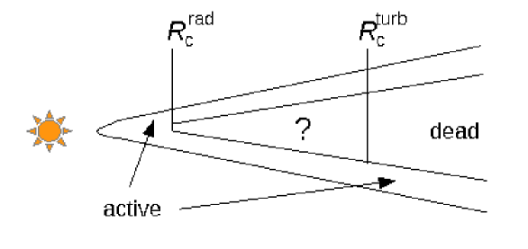
Figure 1: Cartoon of a three zone disk. The very inner radii $R<R_{c}^{\text{rad}}\approx 0.1$ au (and also surface layers) are sufficiently ionised by the star to always support MRI. The outer radii $R>R_{c}^{\text{turb}}\approx 1$ au are always too cold to support the MRI — the turbulence cannot heat the gas sufficiently in this region and it is well shielded from the star. The middle region, sandwiched between the other two could go either way — turbulent or quiescent. It is ‘bistable’. Note that at sufficiently large radii $R\gtrsim 10$ au (not included in the cartoon) the disk may again be fully MRI unstable.

This picture leaves an ambivalent region $R_{c}^{\text{rad}}<R<R_{c}^{\text{turb}}$ sandwiched between the other two. Here the gas can be either quiescent or turbulent. It is bistable. If the gas starts off cold and quiescent it will remain cold and quiescent: the star’s radiation cannot instigate the MRI in this region on its own. But if the gas starts off hot and turbulent it will remain hot and turbulent: the MRI will dissipate heat and this heat will be sufficient to maintain temperatures above the critical limit. The gas can only transfer from one state to the other via a sufficiently large (nonlinear) perturbation.

This is a non-trivial point with potentially important ramifications. It leaves ambiguous the actual location of the dead/active zone boundary, and moreover implies that there may not be a well-defined interface at all. For instance, the gas here may oscillate between the two limits, or exhibit a range of interesting dynamical phenomenon, by analogy with other bistable systems (Zeldovich and McNeill 1985, Murray 2002). More generally, nonsteady behaviour in this region could explain some of the low amplitude accretion variability observed, and will probably be implicated in the dynamics of outburst events, if they are indeed caused by the aperiodic dissolution of the dead-zone (Gammie 1996).

3 A reduced model for the turbulent/thermal dynamics

Our goal is to describe the dynamics in the bistable region of the disk, in particular the interplay between the thermal/ionisation dynamics and the turbulent dynamics. To that end we construct a mean-field model that captures this qualitative behaviour correctly. Our reduced model is rather crude, especially in its treatment of the turbulence, yet it illustrates in a clean way some basic ideas that should govern more advanced models and simulations.

We the define the turbulent amplitude of the disk gas to be

$$K=\tfrac{1}{2}\langle\rho\mathbf{v}^{2}+\mathbf{b}^{2}/(8\pi)\rangle,$$ (6)

where $\mathbf{v}$ and $\mathbf{b}$ are fluctuations in velocity and magnetic field, $\rho$ is density, and the angle brackets denote an azimuthal and vertical average over the disk, as well as an average over short radial scales (see Appendix A). Both $K$ and the gas temperature $T$ are intertwined in the bistable zone: the magnitude of the turbulent amplitude will determine the temperature via turbulent dissipation, but the magnitude of the temperature will determine the ionisation fraction and consequently whether turbulence is present or not. These relationships make up the ‘reaction terms’ in our dynamical model, and have been investigated on their own previously by Balbus and Lesaffre (2008) and Lesaffre et al. (2009). In addition, we add the influence of turbulent diffusion, treating $T$ and $K$ as reactive scalars in a turbulent flow field which both transports and is reacted upon by $T$ and $K$.

In effect, we construct a turbulent closure model with a novel dynamical connection to the thermodynamics. Analogous models have been used in various terrestrial contexts with some success, such as the $k-\epsilon$ turbulence model (for example, Davidson 2000), the multi-scale fluid models (see Frisch 1995 for references), and in mean-field plasma turbulence (for example, Gruzinov and Diamond 1994). Of course, the closest cousin of the model we present is the alpha disk itself, as interpreted by Balbus and Papaloizou (1999), and its more complicated variants (Armitage et al. 2002, Wunsch et al. 2005, 2006, Zhu et al. 2009, 2010). The detailed derivation of our governing equations we give in Appendix A; in the main body of the paper we motivate their main features heuristically. We begin their exposition with a summary of the closely related system in Lesaffre et al. (2009).

3.1 Homogeneous dynamics

Lesaffre et al. (2009) argue that the full equations of viscous and resistive MHD in a shearing box can be effectively modelled by the following simple dynamical system:

$$\frac{dK}{dt} =Q(K,T),$$ (7)

$$\frac{dT}{dt} =\Gamma(K)-\Lambda(T),$$ (8)

where $K$ is the box-averaged turbulent kinetic and magnetic energy, and $T$ is the box-averaged temperature. The evolution of these quantities is controlled by three functions: $Q$, which summarises the growth and saturation of the MRI, $\Gamma$ which represents turbulent heating, and $\Lambda$ which represents radiative cooling. Though these functions can be written as complicated averages over the fluctuating quantities, they may be more simply modelled by physically motivated algebraic expressions. When quantitatively compared to full MHD simulations, this simple system does remarkably well in describing the principle dynamics (Lesaffre et al. 2009), which inspires confidence in its utility.

3.1.1 Parametrising the MRI

To describe the onset and saturation of the MRI via the term $Q$ a simple Landau operator is invoked for a single mode amplitude, which yields

$$Q\approx s\,K-a\,K^{2},$$ (9)

where $s$ is the MRI linear growth rate and $a$ is a parameter associated with its saturation. The temperature influences the linear forcing term, the growth rate, via

$$s=s_{0}[1-\overline{\eta}(T)],$$ (10)

where $s_{0}$ is the ideal MHD growth rate, and $\overline{\eta}$ is the magnetic diffusivity scaled by a constant reference diffusivity. Lesaffre et al. use the Spitzer prescription for $\eta$ but in weakly ionised protoplanetary disks one based on an appropriate Saha equation is required (outlined in Appendix A).

3.1.2 Turbulent heating

The turbulence taps energy stored in the background differential rotation. Turbulent stresses can transform this energy into fluctuations that tumble down a cascade (or pseudo-cascade) into the arms of the dissipation scales where it is degraded into heat. The rate of energy injection into the system is hence proportional to the quadratic correlation $\langle v_{R}v_{\phi}-b_{R}b_{\phi}/(4\pi\rho)\rangle$. Lesaffre et al. approximate this correlation by the turbulent magnitude $K$ (itself a quadratic quantity in the fluctuations) and write

$$\Gamma=w\,K,$$ (11)

where $w$ measures the local shear rate. The greater the local shear the more energy the turbulence can extract. We hence expect $w$ to be a decreasing function of radius, though in most applications we will leave it as a constant.

3.1.3 Radiative cooling

Finally, if we assume that the disk surfaces radiate like a blackbody, the cooling function $\Lambda$ may take the following profile

$$\Lambda=b\,(T^{4}-T^{4}_{\text{eq}}),$$ (12)

where $T_{\text{eq}}$ is the temperature at radiative equilibrium and $b$ is some free parameter associated with the opacity of the gas. It controls, in basic terms, the speed at which radiative equilibrium is enforced. The cooling time is hence $\sim 1/(bT^{3})$, which we expect to be generally much longer than an orbit in the bistable region. A small optical thickness corresponds to a large $b$ and a large optical thickness corresponds to a small $b$. Consequently, $b$ may be a function of $R$ in general. Note that in Lesaffre et al. (2009) a simpler linear cooling was employed.

3.2 Turbulent transport

Equations (7)-(8) describe the average dynamics at a fixed radius in the disk, however our goal is to capture the disk evolution over a significant range of radii and when subject to turbulent transport. Certainly, MRI turbulence effectively moves angular momentum outward, but it will also transport heat, though perhaps less efficiently. The MRI will also tend to spread kinetic and magnetic energy: the more aggressive turbulent fluctuations in higher intensity regions will travel into less turbulently intense regions. The latter transport is analogous to the spreading of kinetic energy away from a region of localised forcing and into unforced quiescent gas. The disordered motions decay as they spread, but these residual motions still have energy distributed over a range of scales which ultimately dissipates.

The simplest way to model the transport of $T$ and $K$ is as a diffusive process. We may then permit $T$ and $K$ to vary with radius $R$, in addition to time, and subsequently erect Fickian diffusion (or ‘eddy viscosity’) terms in both equations (7) and (8). This augmented model would then resemble

$$\frac{\partial K}{\partial t} =Q+\frac{1}{R}\frac{\partial}{\partial R}\left(R\,D_{K}\,\frac{\partial K}{\partial R}\right),$$ (13)

$$\frac{\partial T}{\partial t} =\Gamma-\Lambda+\frac{1}{R}\frac{\partial}{\partial R}\left(R\,D_{T}\,\frac{\partial T}{\partial R}\right),$$ (14)

in which we have introduced diffusion coefficients $D_{K}$ and $D_{T}$. Note that the latter coefficient not only incorporates transport by turbulent eddies but also by radiation. Both $D_{K}$ and $D_{T}$ should be (increasing) functions of the turbulent intensity $K$, and $D_{T}$ may depend on temperature as well. However, for simplicity, we will assume that they are constant.

3.3 Dimensionless equations

The number of free parameters in the system can be reduced by choosing suitable dimensions. We scale time by $1/s_{0}$ which is of order an orbit, and we scale turbulent amplitude $K$ and temperature $T$ by reference values $K_{\text{eq}}$ and $T_{\text{eq}}$. We denote by $K_{\text{eq}}$ the turbulent amplitude in the absence of resistivity (recall that $T_{\text{eq}}$ is the temperature in the absence of turbulence). The quantities $s_{0}$, $T_{\text{eq}}$, and to some extent $K_{\text{eq}}$, may be associated with a prescribed disk radius lying within the bistable region, between 0.1 and 1 au. Next we set the diffusivities

$$D_{T}=L_{T}^{2}\,s_{0}\,\qquad D_{K}=L_{K}^{2}\,s_{0}$$

where $L_{K}$ and $L_{T}$ are the associated diffusion lengths at the prescribed radius. We next scale the unit of length in our equations by $L_{T}$. Together these transformations yield the simpler set of reaction-diffusion equations:

$$\frac{\partial K}{\partial t} =\overline{s}K-K^{2}+P_{r}\,\frac{1}{R}\frac{\partial}{\partial R}\left(R\,\frac{\partial K}{\partial R}\right),$$ (15)

$$\frac{\partial T}{\partial t} =\overline{w}\,K-\overline{b}(T^{4}-1)+\frac{1}{R}\frac{\partial}{\partial R}\left(R\,\frac{\partial T}{\partial R}\right).$$ (16)

Here

$$\overline{w}=\frac{w\,K_{\text{eq}}}{s_{0}\,T_{\text{eq}}},\qquad\overline{b}=\frac{bT_{\text{eq}}^{3}}{s_{0}},$$

and we have defined the Prandtl type number $P_{r}=L_{K}^{2}/L_{T}^{2}$. From Appendix A, we have a growth rate prescription approximating the influence of the Saha ionisation law

$$\overline{s}=\text{tanh}\left[6(T-T_{\text{MRI}})\right].$$ (17)

This means that near the temperature $T_{\text{MRI}}$ the ionisation fraction jumps rapidly to a value sufficient to instigate the MRI. If, in physical units, $T_{\text{eq}}\approx 250$K (associated perhaps with $R=0.5$ au), we have $T_{\text{MRI}}\approx 3.6$. There are now three parameters $\overline{w}$, $\overline{b}$, and $P_{r}$. For notational ease the overlines over $\overline{s}$, $\overline{w}$, and $\overline{b}$ will be suppressed in the following. Finally, we adopt $P_{r}=1$, not only for simplicity but also because we have no numerical estimates for the relative efficiency of turbulent $K$ and $T$ mixing. Thus $L_{T}=L_{K}$. The model offers no detailed quantitative constraints on the two remaining parameters $w$ and $b$, but their meanings are relatively transparent, measuring shear rate and inverse optical thickness, respectively. Because the injection of energy via turbulence proceeds on a time scale longer than an orbit, we take $w<1$. Similarly, the cooling time $1/(bT^{3})$ must be longer than the orbital time. With $T=T_{\text{MRI}}$, this yields $b<0.01$.

3.4 A further simplification: slavery

It is possible to reduce the system (15)-(16) even further if we assume that (a) the time-scale of the MRI saturation is much faster than the thermal timescale, and (b) that the diffusion of $K$ is slow compared to the diffusion of $T$, i.e. $P_{r}\ll 1$. Neither assumption may be strictly true, but the simpler system is particularly convenient to analyse, allowing us an insight into how the more general system works.

These assumptions mean that $K$ is always in equilibrium on the long thermal times that concern us. In other words the turbulent $K$ dynamics are ‘slaved’ to the thermal $T$ dynamics. For long times we have

$$K=\begin{cases}0&\text{if}\quad T\leq T_{\text{MRI}}\\ s&\text{if}\quad T>T_{\text{MRI}}\,.\end{cases}$$ (18)

Now we need only solve one evolution equation, which we write as

$$\frac{\partial T}{\partial t}=\Gamma-\Lambda+\frac{1}{R}\frac{\partial}{\partial R}\left(R\,\frac{\partial T}{\partial R}\right),$$ (19)

where as before the cooling rate is $\Lambda=b(T^{4}-1)$ and now the heating rate is the continuous piecewise function:

$$\Gamma=\begin{cases}0&\text{if}\quad T\leq T_{\text{MRI}}\\ w\,s&\text{if}\quad T>T_{\text{MRI}}\,.\end{cases}$$ (20)

3.5 Caveats

Before applying the model we should stress a few points regarding some of its weaknesses, especially with respect to its simplistic treatment of the turbulence. As is made clear in Appendix A, the validity of the model rests on the soundness of averaging over the small-scale disordered motions of the MRI turbulence, in addition to the vertical thickness of the disk. In particular, it demands a clean separation between large scales of at least $H$, upon which global disk properties manifest, and the short MRI turbulent scales. Stratified simulations of the MRI suggest this is only marginally true at best (Davis et al. 2010, for example), while near criticality the fastest growing mode varies on approximately $H$. We believe this problem will not derail the qualitative results.

In addition, for the small scale averages to make sense, the fluctuations need to be well-behaved — they cannot be subject to intermittent and volatile outbursts or other critical behaviour. Yet that is what we might expect from the marginal MRI! The best we can hope for is that this bad behaviour does not invalidate the predictions of the mean-field model — that, in fact, the model indeed does a decent job of describing the mean dynamics, even if the fluctuations around that mean are a little wild at times.

One should also add that the eddy viscosity description of turbulent flow has long been known to be at best a crude, and sometimes misleading, approximation. In reality the stress exerted by such flows are non-Newtonian, sometimes exhibiting a nontrivial dependence on the shear rate, effects associated with their finite relaxation time, and even negative transport (see, for example, Frisch 1995, Davidson 2000). That all said, we are interested only in the basic dynamics, which we believe are independent of the particulars of the turbulence itself.

A final issue is the vertical averaging: in doing this, we are discarding any information about how the disk thickness responds to local changes in either the turbulence or temperature. It is implicitly assumed that $H$ varies passively with changes in $T$. For example, a transition between the hot MRI active region and a cold quiescent region will be characterised by a drop in $H$, meaning the inner turbulent radii of a protostellar disk may bulge. Any interesting stability problems, or other dynamics, that might arise from this configuration cannot be captured by the model.

4 Analysis of homogeneous states

4.1 Local states

Our first task is to compute homogeneous steady states — i.e. equilibrium states with no radial structure, which describe either dead or active zones. As in a shearing box, such equilibria we expect to hold locally in a protoplanetary disk. Because the diffusion terms take no part in these calculations, we need only solve a coupled pair of ODEs.

The steady-state equations to be solved are:

$$sK-K^{2}=0,\qquad w\,K-b(T^{4}-1)=0,$$ (21)

which arise directly from Eqs (15)-(16). The first equation matches the linear forcing by the MRI to its saturation through the quadratic term. The second equation matches the first turbulent heating term with the second radiative cooling term.

This system admits the cold quiescent (dead) state

$$K=0,\qquad T=1.$$

Turbulence is absent and the gas falls into radiative equilibrium. The system also potentially admits turbulent states $K>0$, with $K=(b/w)(T^{4}-1)$ and with the temperature determined from the nonlinear algebraic equation

$$w\,s=b(T^{4}-1),$$ (22)

with $s$ given by Eq. (17). Here the heating rate $\Gamma=w\,s$ is on the left and the cooling rate $\Lambda=b(T^{4}-1)$ on the right. Naturally, the linear growth rate $s$ must be positive for this to work or else there is no turbulent heating at all. Note also that the equilibrium depends on a single parameter, the ratio $b/w$.

Equation (22) must be solved numerically. But if we plot the heating and cooling as functions of $T$ we can get a good idea of how the balances work. Examples are given in Fig. 2 for three representative values of $b/w$. The points at which the two curves cross correspond to turbulent/thermal equilibria. Note that, depending on the ratio $b/w$, we can achieve one solution (the cold quiescent state), two solutions, or three solutions. In the figure we plot these three different cases. The critical $b/w$ value above which turbulence vanishes, and for which there is only the dead state, is approximately $0.0042$. When $b/w>0.0042$ the cooling rate is too efficient, and/or the amount of free energy insufficient, for the requisite MRI temperatures to be maintained. Naturally we associate the cold quiescent state with a dead zone, and the hotter of the two turbulent state with the active zone. The intermediate state we show later is unstable and will not be observed, though it is important in policing the boundary between the other equilibria.

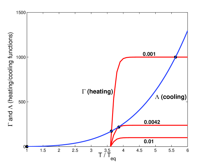
Figure 2: Heating and cooling as functions of temperature $T$ for different ratios of $b/w=0.001,\,0.0042,0.01$. Crossings correspond to thermal equilibria and are marked with black dots. These comprise the cold quiescent state $T=1$, and up to two turbulent states: $T_{I}$ (which we term the ‘intermediate state’) and $T_{A}$ (which we call the ‘active state’). The former is unstable and the latter is stable.

Another way to characterise the equilibria is to rewrite Eq. (22) as

$$T=\left[1+(w/b)s\right]^{1/4}.$$

Because $s$ is essentially a step-function in $T$, and the upper turbulent solution always occurs when resistivity has been virtually ‘switched-off’, we can approximate the upper state $T_{A}$ by

$$T_{A}\approx(1+w/b)^{1/4},\qquad K_{A}\approx 1.$$ (23)

Therefore, the greater the parameter combination $w/b$ the greater the active zone temperature $T_{A}$. This makes sense because $w/b$ measures the amount of heat stored in the gas. Recall $b$ represents the ability of the gas to hold heat (optically thick gas takes smaller $b$) while $w$ controls the amount of heat generated via turbulence ($w$ is larger when more energy is available to be dissipated). Optically thicker gas at smaller radii is hotter, whereas optically thinner gas at larger radii is colder.

4.2 Linear stability

Next we briefly inspect the stability of the three possible steady states. We find that the quiescent state $K_{Q}=0$, $T_{Q}=1$ is always stable on account of its cooling law (heating is absent around this state). The upper turbulent state $K_{A}\approx 1$, $T_{A}\approx(1+w/b)^{1/4}$ is also stable. This is easy to see from the heating and cooling functions in Fig. 2. If the temperature increases from the hotter active state the cooling function will be greater than the heating function: the excess temperature will be removed and the system will return to equilibrium. On the other hand, if the temperature decreases then heating will dominate cooling and the gas will also return to equilibrium. It is quite the opposite for the intermediate equilibrium: a small positive deviation in temperature means that heating will dominate cooling and so the gas will continue heating up. Similarly a small negative deviation means that cooling will dominate.

This heuristic reasoning can be confirmed with a detailed linear stability analysis, which we present in Appendix B. The linear dispersion relation that ensues gives the following stability criterion

$$\frac{d\Lambda}{dT}>\frac{d\Gamma}{dT},$$ (24)

which puts in mathematical terms the graphical argument presented earlier. Direct substitution of $\Gamma=wK$ and $\Lambda=b(T^{4}-1)$ shows that the quiescent state and the upper active state are always stable, while the intermediate state is not. It is, in fact, a saddle point with one stable and one unstable mode (manifold).

4.3 Nonlinear homogeneous dynamics

Lastly, we describe the nonlinear dynamics of the homogeneous equations. This situation might mimic conditions in a localised patch, as approximated by a shearing box (cf. Lesaffre et al. 2009). The full dynamical system here is:

$$\frac{dK}{dt} =s\,K-K^{2},$$ (25)

$$\frac{dT}{dt} =w\,K-b(T^{4}-1),$$ (26)

two nonlinear ODEs in time, which we solve numerically using a Runge-Kutta method. In Fig. 3 a number of numerical solutions to this system are plotted alongside the vector ‘reaction’ field $\mathbf{R}$ which controls the solution trajectories:

$$\mathbf{R}=[s\,K-K^{2},\,w\,K-b(T^{4}-1)].$$ (27)

The three equilibrium points are represented by black spots.

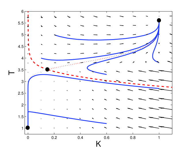
Figure 3: Phase portrait of the homogeneous problem. Some solutions of Eqs (25) and (26) are plotted in blue along with the reaction vector field in black. The three equilibrium solutions are represented by black dots. In addition, the stable and unstable manifolds of the intermediate state are plotted as dashed and dotted lines respectively. Trajectories which begin above the dashed line (the stable manifold) end up at the turbulent state, and trajectories which begin below the dashed line end up in the dead state. The average time it takes to reach either state is limited by the cooling time. A trajectory settles on the hot turbulent state in some 10 orbits, whereas one approaches the quiescent state in over 100 orbits. Parameters are $w=1$, $b=0.001$.

As is clear, trajectories eventually end up on one of the stable states. The speed at which the system moves to one or the other state is limited by the cooling rate $\sim bT^{3}$. Most trajectories are first attracted to the unstable saddle point, guided along its stable manifold (the red dashed curve), but are finally repelled along the stable manifold (the dotted curve). Which state they terminate upon depends on where in the phase space they begin and, more specifically, in which basin of attraction they initially fall.

The phase space can be divided into two regions, the basin of attraction of the quiescent dead state, and that of the active turbulent state. The boundary between the two is given by the stable manifold of the intermediate state (the dashed curve). As the parameters change, this boundary also changes, with the basins of attraction growing or shrinking relatively. In particular, as $b/w$ decreases the intermediate state approaches the low state, thus diminishing the basin of attraction of the low state.

5 MRI-fronts

We have dealt with the homogeneous dynamics of our reduced model, first detailing the equilibrium states the system admits, their linear stability, and the ensuing nonlinear dynamics. The analysis has been limited to gas at a particular radius, allowing the gas to settle on either an active or dead state. But, as we vary the radius in the disk, the gas presumably transitions from one state to the other at some sort of interface. In this section we attempt to compute ‘fronts’ connecting these two stable homogeneous equilibria. We hence must reinstate the spatial element of the nonlinear problem.

5.1 Equations in a semi-local model

In order to best study a nonlinear front solutions we concentrate on a small finite region at a certain radius $R_{0}$ in the disk. We assume that any kind of front structure will be much shorter than the local radius. We hence drop the term arising from the cylindrical geometry in Eqs (15)-(16). We also introduce an intermediate radial variable $X$ so that

$$X=R-R_{0}.$$

The equations are now

$$\frac{\partial K}{\partial t} =s\,K-K^{2}+\frac{\partial^{2}K}{\partial X^{2}},$$ (28)

$$\frac{\partial T}{\partial t} =w\,K-b(T^{4}-1)+\frac{\partial^{2}T}{\partial X^{2}}.$$ (29)

Next we make the following ansatz: there exists a front with a radial profile that is steady and which moves radially at a constant speed $c$. This front connects the stable quiescent equilibrium state $(K_{Q},\,T_{Q})$ and the stable turbulent state $(K_{A},\,T_{A})$. Because of radial disk structure, the assumptions of constant $c$ and steady profiles only hold approximately in our small region near $R_{0}$. However, they permit us to directly compute the fronts and to clearly examine their properties. We relax these assumptions later in numerical simulations.

To make progress we move into a frame comoving with the front, and introduce the comoving spatial variable

$$\xi=X-c\,t.$$ (30)

In this frame the front profile is stationary and thus $K=K(\xi)$ and $T=T(\xi)$. The partial differential equations (28)–(29) become the coupled ordinary differential equations

$$\frac{d^{2}K}{d\xi^{2}}+c\frac{dK}{d\xi}+s\,K-K^{2}=0,$$ (31)

$$\quad\frac{d^{2}T}{d\xi^{2}}+c\frac{dT}{d\xi}+w\,K-b(T^{4}-1)=0.$$ (32)

The boundary conditions for these equations come from the requirement that the front must connect $(K_{Q},\,T_{Q})$ with $(K_{A},\,T_{A})$. Formally at least, this may be written as

$$K\to K_{Q},\quad T\to T_{Q}\quad\text{as}\quad\xi\to\infty,$$ (33)

$$K\to K_{A},\quad T\to T_{A}\quad\text{as}\quad\xi\to-\infty.$$ (34)

A more compact vector form for the equations (31) and (32) is

$$\frac{d^{2}\mathbf{z}}{d\xi^{2}}+c\frac{d\mathbf{z}}{d\xi}+\mathbf{R}=0$$ (35)

where we haved introduced the solution vector $\mathbf{z}=[K,\,T]$. Recall that $\mathbf{R}$ is the reaction field introduced in (27). It corresponds to the trajectory arrows in Fig. 3.

Equations (31)-(34) describe a one-dimensional nonlinear eigenvalue problem for $K$ and $T$ with eigenvalue $c$. These equations must be solved numerically. We give the results of such computations in a following subsection. But first we prove some results concerning the direction of front propagation.

5.2 Direction of front propagation

The hypothetical front solution may not be static. But in which direction will it move and at what speed? If it connects a quiescent state to a turbulent state, will it move into the turbulent state $(c<0)$ or will it move into the quiet state $(c>0)$? Later, it is shown numerically that either case is possible. In this section we try and provide some arguments for why this is so and offer some analytic predictions for what sign $c$ will take.

The main ideas can be best illustrated using the simple ‘slaved’ system introduced in Section 3.4. Upon imposing the assumptions of the previous subsection, the governing equation (19) becomes

$$\frac{d^{2}T}{d\xi^{2}}+c\frac{dT}{d\xi}+\Gamma-\Lambda=0,$$ (36)

Multiplying by $dT/dz$ and integrating, one gets

$$c=-\frac{\int_{-\infty}^{\infty}(\Gamma-\Lambda)\partial_{\xi}T\,d\xi}{\int_{-\infty}^{\infty}|\partial_{\xi}\,T|^{2}d\xi}.$$ (37)

and so

$$\text{sgn}(c)=\text{sgn}\int_{T_{Q}}^{T_{A}}(\Gamma-\Lambda)\,dT.$$ (38)

This tells us that the sign of $c$ depends on the ‘area’ (in $T$-space) that lies beneath the combined heating and cooling rates.

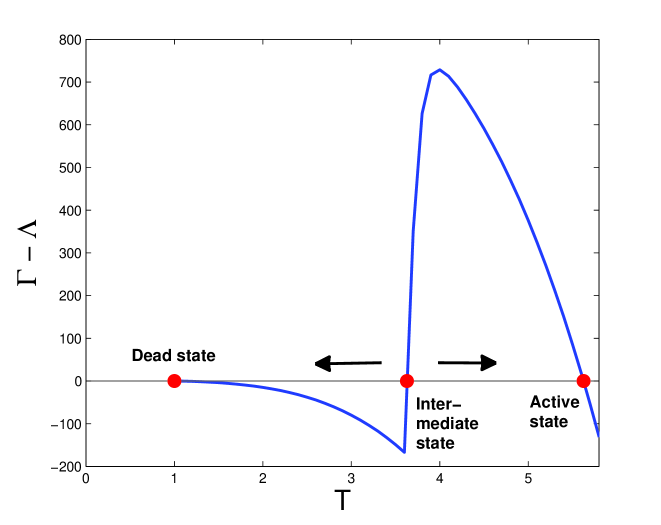
Figure 4: The combined heating and cooling rate as a function of temperature for the slaved model. Arrows indicate the direction in which gas will tend to move if subject to the thermal dynamics. We can easily see the two basins of attractions of $T_{Q}=1$ and $T_{A}$, with the intermediate state acting as the boundary between them.

The combined heating and cooling $(\Gamma-\Lambda)$ is plotted in Fig. 4. Quite generally there will be two opposing contributions to the area under this curve (the integral in (38)). There will be a positive contribution from the portion of the front lying near $T_{A}$, in the active state’s basin of attraction. And there will be a negative contribution from the portion of the front near the lower quiet state, in its basin of attraction. Because the slaved model is only 1D, these two basins are easy to see. Gas that is a little hotter than the intermediate state is drawn to the upper turbulent state, while gas a little colder is drawn to the lower state: this is represented in Fig. 4 by the horizontal arrows. For the parameters chosen here the contribution from the active state’s basin dominates and $c>0$.

Even if the integral in Eq. (38) were intractable, we can at least say that the relative sizes of the two basins of attraction help determine the sign of $c$. For example, if the parameter $b/w$ is very small then $T_{A}=(1+w/b)^{1/4}$ will be large, and consequently the basin of attraction of the upper active state will also be large. We would then expect the integral (38) to be dominated by this region and for $c$ to be positive. On the other hand, if $b/w$ is continuously decreased so that $T_{A}$ approaches the intermediate state, then its basin of attraction will also decrease. At a second critical $b/w$ one would expect the sign of $c$ to change from positive to negative.

These heuristic arguments can be worked through in some detail because (38) is integrable once we treat the heating $\Gamma$ as essentially a step function (cf. Section 4.1). We find

$$\int_{1}^{T_{A}}(\Gamma-\Lambda)dT\approx\tfrac{1}{5}\,b\,T_{A}^{5}-(b+w)T_{A}+w\,T_{\text{MRI}}+\tfrac{4}{5}\,b,$$

in which $T_{A}\approx(1+w/b)^{1/4}$. This equation permits us to calculate the critical value of $b/w$ at which point $c=0$, as a function of $T_{\text{MRI}}$. The equation corresponding to $c=0$ is

$$(1+w/b)^{5/4}-\tfrac{5}{4}(w/b)\,T_{\text{MRI}}-1=0,$$ (39)

which must be solved numerically. However, because $b/w$ is small, a reasonable approximation can be obtained by expanding the first bracketed term. This gives

$$(b/w)_{\text{cr}}\approx(5\,T_{\text{MRI}}/4)^{-4}\approx 0.0025.$$

It is easy to see that the system admits two families of MRI-fronts. When $(b/w)<0.0025$ we have an outward moving front, $c>0$. When $0.0042>(b/w)>0.0025$ we have an inward moving front, $c<0$. And when $(b/w)>0.0042$, there is no front at all (because there is no active state available, cf. Section 4.1). Later we discuss how this parameter configuration $b/w$ depends on disk radius and, consequently, how an MRI-front changes as it propagates through the disk. The fact that there is a value for $b/w$ for which $c=0$ means that there is likely a special radius at which $c=0$, and hence an attracting radius towards which all fronts migrate.

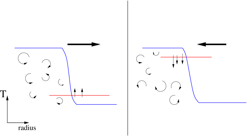
Figure 5: Simple cartoon of the temperature profile of two fronts. The red line overlaying them indicates the critical temperature separating the two basins of attraction of the hot/turbulent and cold/quiescent states.

Finally, we may obtain a better physical understanding on the sign of $c$ through the following argument. In Fig. 5 we plot two hypothetical MRI-front profiles for the temperature $T$. Overlying these profiles is a red line which corresponds to the critical temperature $T_{I}$ separating the basins of attraction of the quiet and the active states. In the first picture the majority of the gas lies within the active zone’s basin. Quiescent fluid heavily perturbed by the neighbouring front will find itself more likely to be pushed over this critical threshold than fully turbulent fluid: the hot turbulent fluid will have to cool off much more than the cold fluid has to heat up. As this fluid heats up and becomes turbulent the front moves forward ‘gobbling’ up this gas, and hence moves further into the quiescent state — the large black arrow. In the second picture the situation is reversed and the MRI-front ‘retreats’ into the turbulent gas.

5.3 Numerical examples of MRI-fronts

Having listed some analytic results in certain limits which help us understand the nature of the dead-zone/active-zone interface, we now compute these solutions explicitly from Eqs (31)-(34) using a numerical scheme. The problem is a 4th order nonlinear eigenvalue problem in one variable $\xi$, and we expect the system to be quite stiff: the profiles will not change much over most of the domain except near the transition front where they will vary rapidly. As a consequence, we employ a relaxation method, whereby an initial guess to the front profile and an initial guess for $c$ are gradually ‘evolved’, via Newton’s method, to a numerical approximation of the correct solution (Press et al. 2007).

5.3.1 MRI-front profiles

We show results for which $b=0.001$ and $w$ varies. MRI-fronts travelling either inward or outward are supported by the equations. Two examples are plotted in Figs 6 and 7. In both cases the front joins the active and dead-zones smoothly over a characteristic lengthscale. For most outward propagating fronts, the radial scale of the transition region for both $K$ and $T$ is roughly $3L_{\text{T}}$. However, slower moving fronts (in either direction) or stationary fronts exhibit a temperature transition with a long ‘tail’ that extends tens of $L_{\text{T}}$ into the dead-zone.

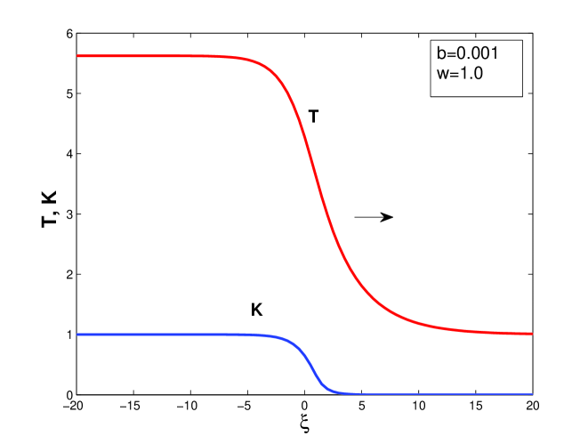
Figure 6: MRI-front profile with $P_{r}=1$, $b=0.001$, $w=1$. The front speed is $c=0.28L_{T}\Omega$, so the front travels into the dead-zone, i.e. outward.

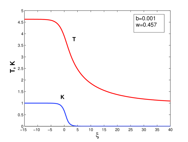
Figure 7: MRI-front profile with $P_{r}=1$, $b=0.001$, $w=0.457$. The front speed is almost zero $c=9.3\times 10^{-4}L_{T}\Omega$. Note the extended morphology of the temperature transition in comparison to $K$.

5.3.2 Front velocities

Whether the front travels inward or outward its speed $c$ is bounded according to $|c|<L_{T}\Omega<H\Omega$, and is thus controlled by the largest turbulent eddies; naturally, the front cannot travel faster than one diffusion length per orbit. The fastest fronts are those with larger $w$, i.e. originating deeper in the active zone at small radii. These may travel outward as fast as a disk scale height $H$ per orbit: roughly 1 au in less than 10 years. However, $c$ will vary as the front travels because of the dependence of the parameters ($w$ especially) on radius, as well as the physical scales $\Omega$ and $H$.

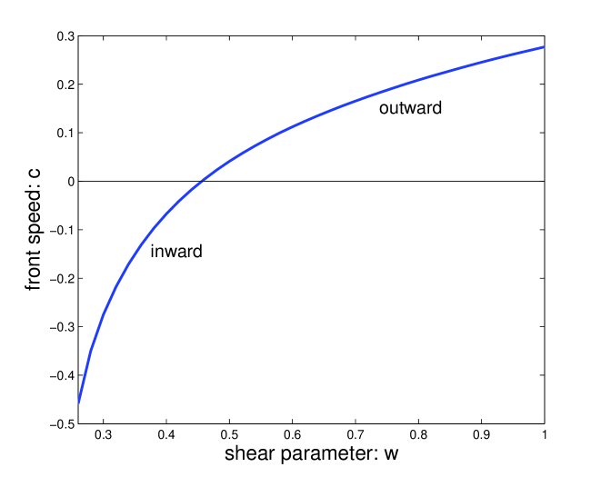
Figure 8: Front speed $c$ as a function of the parameter $w$. Other parameters are held constant, namely $b=0.001$. As $w$ decreases so does $c$ until at a critical point $c=0$, after which $c$ is negative and the front propagates inward. The critical $w$ is approximately $w=0.4563$.

In Fig. 8, we show how the front speed $c$ changes as we vary the shear parameter $w$, keeping $b$ fixed. As $w$ decreases so does $c$ until at a critical point $c=0$ after which $c$ is negative and the front propagates inward. At a second value of $w$ the front ceases to exist: the upper turbulent state vanishes and the gas is no longer bistable. This behaviour adheres to our expectations given the simple slaved system of Section 5.2. There the critical value of $b/w$ is 0.0025, at which point $c=0$. The more general system here yields a value closer to 0.0022, which is in fair agreement.

We associate smaller $w$ values with larger radii (less shear) and larger $w$ with smaller radii (greater shear). It is expected then that fronts originating at larger radii propagate inwards and fronts coming from smaller radii propagate outwards. In between there is a critical radius $R_{\text{att}}$ at which point $c=0$ and the front stays put. It follows that all MRI-fronts are attracted to this special radius. And this radius by necessity lies within the bistable region: $R_{c}^{\text{rad}}<R_{\text{att}}<R_{c}^{\text{turb}}$. Consider a front that begins near the inner edge of the bistable zone $R_{c}^{\text{rad}}$. It will travel outward at some initial speed, but as it approaches $R_{\text{att}}$ it will decelerate; eventually it will slow to a crawl and come effectively to a halt near this radius. On the other hand, a front that begins near the outer boundary of the bistable zone $R_{c}^{\text{turb}}$ will propagate inwards until it too approaches $R_{\text{att}}$, at which point it slows down and eventually stops.

6 Travelling fronts in global disk models

In this section the physics explored in the previous sections are tested in simulations of the full equations (15)–(16) in a simple global disk model. As we have argued, an MRI-front usually does not linger in one place; it will by its nature move away to radii where the properties of the gas are going to be different to where it started, and consequently where its profile and speed will change. How this works in detail can only be captured by a calculation that take into account the radial structure of the disk.

The geometric cylindrical terms are reinstated in (15)–(16) and the disk’s radial structure is encoded through the dependence of the cooling and shear parameters $b$ and $w$ on radius $R$. By setting $w\propto\Omega$ and recognising that the cooling time decreases with radius, we suggest the following model

$$w=w_{0}\left(\frac{R}{R_{c}^{\text{turb}}}\right)^{-3/2},\qquad b=b_{0}\left(\frac{R}{R_{c}^{\text{turb}}}\right)^{p},$$ (40)

where the constants $w_{0}$ and $b_{0}$ correspond to the critical values for which there are no active states, and at which point $R=R_{c}^{\text{turb}}$. Recall from Section 3, that this occurs when $b_{0}/w_{0}=0.0042$. The power $p\geq 0$ we are free to set, but given the uncertainties in the opacity in the inner disk we set $p=0$ in most applications. In addition, we should let $T_{\text{eq}}$ also be a function of $R$ because of heating from the central star. This aspect of the problem is neglected mainly for ease, and also because appreciable change in $T_{\text{eq}}$ should be limited to near the inner disk edge.

The equations (15)–(16) are simulated with a finite-difference scheme and explicit first order time-stepping over a radial domain extending from 0.1 au to 5 au. Space units are chosen so that $R_{c}^{\text{turb}}=2$ au and $L_{T}=0.1$ au. Time is scaled by the orbital period at $R_{c}^{\text{turb}}$. Various initial conditions were trialed, including simple tanh profiles. But all yielded the same long term equilibrium.

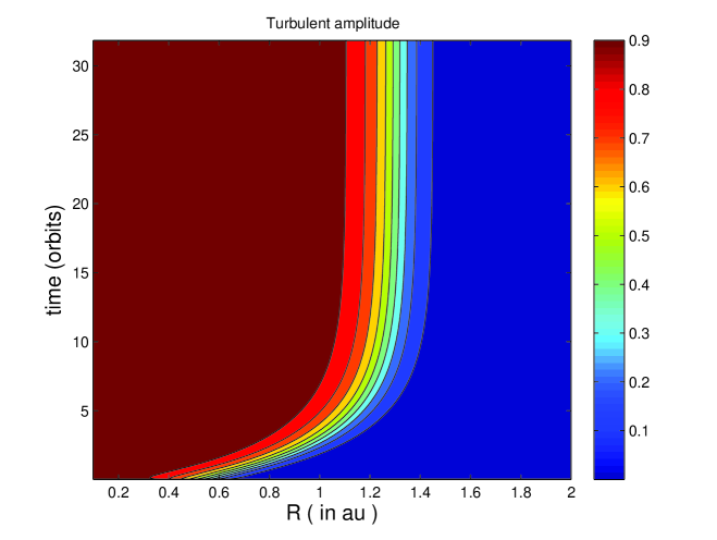
Figure 9: Space-time diagram of the evolution of the turbulent amplitude $K$ in a global model of a protoplanetary disk. The front propagates from near the inner edge and settles near the radius $R_{\text{att}}$, which is some 65 % of $R_{c}^{\text{turb}}=2$ au.

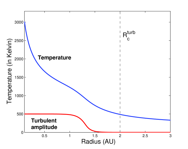
Figure 10: Long time equilibrium of the temperature field in a global model of a protoplanetary disk. Superimposed on the figure is the turbulent amplitude rescaled by a factor 500 so as to be visible.

In Fig. 9 we plot a typical space-time diagram of the turbulent amplitude $K$. The front is released at a small radius, near the inner edge, from where it propagates outward rapidly, covering 0.6 au in less than 5 orbits. It then slows down as it approaches the critical radius $R_{\text{att}}$ and eventually comes effectively to a halt. In Fig. 10 we plot a snapshot of the long time temperature profile, obtained after 200 orbits. The front is completely stationary at this point. Note that, unlike the turbulent amplitude, the temperature $T$ varies with radius even far from the location of the front. This is because the turbulent equilibrium state $T_{A}$ is a function of radius through $w$. Thus at smaller radius the turbulent heating is greater, as is $T_{A}$ (cf. (23)). Note that the model appears to overestimate $T$ at these small radii in comparison with alpha models (see e.g. Terquem 2008). Superimposed upon the figure is the turbulent amplitude, scaled appropriately.

In these figures, and more generally, the final location of the front $R_{\text{att}}$ is roughly 65% of $R_{c}^{\text{turb}}$. This could be pre-empted from Eq. (40), once we recognise that $b/w=0.0022$ at this radius. Then we have the estimate

$$\left(\frac{R_{\text{att}}}{R_{c}^{\text{turb}}}\right)=\left(\frac{0.0022}{0.0042}\right)^{2/(3+2p)},$$ (41)

which gives $\approx 0.65$ when $p=0$. For $p>0$ the attracting radius is greater.

Finally, the front profiles we have simulated appear to be stable even when they slow to a static equilibrium. The simulations show no evidence of secondary instability and a subsequent dissolution into more disordered time-varying dynamics as witnessed in, for example, flame fronts (Zeldovich and McNeill 1985). Neither is there any sign of the instability uncovered by Wunsch et al. (2005, 2006). If such instabilities exist in real protoplanetary disks, our model is too simple to capture them, omitting, for example, accretion. But there is also the question of consistency. Our model, and the related alpha disk models, have been derived via averaging over small-scale fluctuations, and have thus assumed that these fluctuations are well-behaved and bounded. The issue of front instability and more complicated time-dependent behaviour must be settled by direct numerical simulations of the MRI itself.

7 Summary and discussion

We now summarise the contents of the paper and bring out its most important points. In Section 2, we made the case that in most protostellar disk systems, midplane gas at inner radii (less than about 1 au) finds itself bistable: it can be either quiescent or MRI-turbulent. As a consequence, the location of the dead/active zone boundary may be difficult to pin down and, moreover, the boundary profile itself not particularly defined. Estimates on the critical radii which bound this gas are not well constrained; but we expect the inner radius $R_{c}^{\text{rad}}$ to be (much) less than 0.1 au, and the outer radius $R_{c}^{\text{turb}}$ to be roughly 1 au, with its exact value dependent on stellar mass and accretion rate.

In order to understand this region, a reduced model was introduced (Section 3) which describes the mutual coupling of the turbulent and thermal dynamics of the gas in the bistable region. The turbulence is modelled in a mean-field fashion, which assumes that its fluctuations are well behaved: large amplitude intermittent behaviour (which might be quite important) is smoothed out. The governing equations take the form of two reaction-diffusion equations for temperature and turbulent amplitude. After a suitable rescaling, the remaining free parameters have relatively transparent meanings: $b$ represents the local gas opacity, and $w$ represents the local shear.

In Section 4, we set this model to work computing homogeneous equlibrium states, in particular showing that in the bistable zone of a disk there should be three equilibria: the dead-zone state and the active turbulent state (both stable as expected) in addition to an intermediate state that is unstable and which polices the boundary between these two outcomes.

In Section 5 we compute what we call ‘MRI-fronts’, which are travelling transitions connecting the active zone to the dead zone. We can prove a number of properties about these fronts. Of greatest importance is the sign of the front speed: we show that fronts beginning at the inner edge of the bistable zone propagate outward, while fronts beginning at the outer edge of the same zone travel inwards. There then exists a critical radius $R_{\text{att}}$ at which point the MRI-front velocities are precisely zero and it is towards this radius that all fronts must go and finally anchor themselves. This is the true effective boundary between active and dead zones. Numerical simulations of the equations in a global model of a protoplanetary disk are given in Section 6 and these confirm this expectation. They also show that the front solutions are stable to secondary perturbations, at least within the confines of our model assumptions.

So where does this leave us? Our simple system predicts that the interface between MRI-active and inactive regions is in fact a robust and coherent feature that relaxes into a steady profile. Large deviations from this steady equilibrium will decay and the MRI-front will ultimately return to its halting radius $R_{\text{att}}$. This critical radius can be somewhat less than existing estimates, but the idea that there exists a well-defined boundary still applies. The picture that we have developed is certainly favourable to planet formation scenarios that rely on a stable and quasi-static dead/active zone interface. If the interface is as robust as suggested by the model, its associated pressure inhomogeneity may be equally robust and long-lived: precisely what is required for the accumulation and eventual agglomeration of solid material.

However, the model has neglected (in fact, ‘averaged away’) the highly intermittent turbulent fluctuations that we expect such an MRI-front to suffer. The smooth profiles that we have generated (Figs 6 and 7) represent an average; in reality, an MRI front will most likely be a disordered structure subject to potentially large amplitude perturbations. Moreover, it is not quite clear what lengthscales this disorder encompasses – it will probably be on a scales of order the transition scale itself – some fraction of $H$. If the transition region is indeed volatile and fairly broad then it may inhibit the development of the pressure inhomogeneity required by planet formation theories. Moreover, additional physics (accretion, for example) and realistic vertical structure may stimulate instability and associated secondary fluctuations. A sensible way to check some of these effects is to better describe the turbulent dynamics and move on from the diffusive approximation. MHD simulations of the MRI with a temperature dependent resistivity are needed. These might be undertaken in cylindrical geometry, which is sufficient to capture the key global effects (with shear rate declining with radius), while allowing acceptable resolution, given modern computational constraints. Such simulations are planned and will be presented in later work.

Appendix A Derivation of the mean-field model

Though the mean-field model used throughout the main paper can be motivated by physical heuristic arguments, its general lineaments can formally be derived through a separation of scales analysis. In this appendix we briefly sketch out the procedure.

A.1 Governing equations

We begin with the full equations of resistive and viscous MHD

$$D_{t}\rho=-\rho\,\nabla\cdot\mathbf{u},$$ (42)

$$D_{t}\mathbf{u}=-\nabla\Phi-\frac{1}{\rho}\left(P+\frac{B^{2}}{8\pi}\right)+\frac{1}{4\pi\rho}\mathbf{B}\cdot\nabla\mathbf{B}+\frac{1}{\rho}\nabla\cdot\mathbf{\Pi},$$ (43)

$$D_{t}\mathbf{B}=\mathbf{B}\cdot\nabla\mathbf{u}-\mathbf{B}\,\nabla\cdot\mathbf{u}+\eta\nabla^{2}\mathbf{B},$$ (44)

$$E\,D_{t}S=\rho(\psi_{\text{dis}}+\psi_{\text{ext}})-\nabla\cdot\mathbf{F},$$ (45)

where $\rho$ is volumetric mass density, $\mathbf{u}$ is velocity, $\Phi$ is the gravitational potential of the star, $P$ is pressure, $\mathbf{B}$ is magnetic field, $\mathbf{\Pi}$ is the (molecular) viscous stress tensor, $\eta$ is the resistivity, $E$ is the internal energy density, $S=\ln P\rho^{-\gamma}$ is the entropy function and $\gamma$ the ratio of specific heats, $\rho\psi_{\text{dis}}$ comprises viscous and resistive heating, and $\rho\psi_{\text{ext}}$ represents external heating from the star. Finally, the radiative flux is denoted by $\mathbf{F}$. We also have denoted the total derivative by $D_{t}=\partial_{t}+\mathbf{u}\cdot\nabla$. In writing the above we have assumed an ideal gas equation

$$P=\frac{\mathcal{R}}{\mu}\,\rho\,T$$ (46)

where $\mathcal{R}$ is the gas constant and $\mu$ is mean molecular weight. It follows that $E=P/(\gamma-1)$. We set the resistivity to be a function of temperature $\eta=\eta(T)$ via an appropriate form of Saha’s equation (see Stone et al. 2000 and Balbus 2011). This means that we are considering thermal ionisation explicitly. We neglect non-thermal ionisation.

A.2 Fluctuations

We assume that equations (42)-(45) admit a laminar equilibrium state characterised by (near) Keplerian rotation:

$$\mathbf{u}=\mathbf{u}_{0}(R)=R\Omega(R)\,\mathbf{e}_{\phi}$$

where $R$ is cylindrical radius (the tiny radial drift arising from molecular viscous torques we omit). There will also be some radial and vertical structure in the variables $\rho$ and $P$, which won’t be listed. Finally, we assume that there is a weak magnetic field $\mathbf{B}_{0}$ that does not influence the equilibrium balances significantly but which plays the defining role in the disk’s stability by catalysing the MRI.

In a given region of this disk the MRI will occur if the local resistivity is sufficiently low. We next assume that in such an unstable region turbulence will ensue, giving rise to both magnetic and velocity fluctuations which we denote by $\mathbf{v}$ and $\mathbf{b}$. Because MRI turbulence is mainly subsonic, associated density fluctuations are considered to be small and are neglected.

The velocity fluctuations are small compared to the Keplerian motion $|\mathbf{v}|\ll|R\Omega|$ and inhabit a well-defined range of lengthscales, the upper bound of which we denote by $l$, understood as either the main energy injection scale of the MRI, or the scale of the largest turbulent eddies. We then posit the following hierarchy $l\ll H\ll R,$ where $H$ is the disk semithickness. The first scaling is marginally true at best, and in fact we can only probably say $l<H$, but the stronger form is necessary for the mathematical argument to go through. This motivates the introduction of the small parameter $\epsilon=l/H.$

A.3 Fluctuation equations

The magnitude of the fluctuations is defined through

$$k=\tfrac{1}{2}[\rho\mathbf{v}^{2}+\mathbf{b}^{2}/(8\pi)]$$

which we term the ‘turbulent amplitude’ or ‘intensity’. One can derive an evolution equation for $k$ from Eqs (42)-(45). This can take multiple forms (see for example Balbus and Hawley 1998). We use the following:

$$\partial_{t}k+\nabla\cdot\left(\mathbf{v}\,k\right)=q,$$ (47)

where the source term $q$ is rather ungainly. It can be written as

$$q =\mathbf{v}\cdot(\nabla\cdot\mathbf{\Pi})-\mathbf{v}\cdot\nabla P-\nabla\cdot\left(\mathbf{u}_{0}\,k\right)$$

$$\hskip 56.9055pt+\frac{1}{4\pi}\left[\eta\mathbf{b}\cdot\nabla^{2}\mathbf{b}+\mathbf{v}\cdot(\mathbf{v}\cdot\nabla\mathbf{u}_{0})\right.$$

$$\left.+\mathbf{b}\cdot(\mathbf{b}\cdot\nabla\mathbf{u}_{0})+(\mathbf{b}+\mathbf{B}_{0})\cdot\nabla(\mathbf{b}\cdot\mathbf{v})-\mathbf{v}\cdot\nabla(\mathbf{B}_{0}\cdot\mathbf{b})\right].$$ (48)

This $q$ term is obviously an exceedingly complicated function of $k$. It both controls the emergence of the MRI and its nonlinear saturation through turbulence. Note that it also depends explicitly on temperature through $\eta$, and to a lesser extent $P$.

In addition, we can derive an equation for fluctuations in internal energy or temperature. It is more convenient, however, to deal with the total temperature $T$. It is

$$\partial_{t}T +\nabla\cdot\left(\mathbf{v}\,T\right)=-\nabla\cdot(\mathbf{u}_{0}\,T)+(2-\gamma)T\nabla\cdot\mathbf{u}$$

$$\hskip 19.91684pt+\frac{(\gamma-1)}{\mathcal{R}/\mu}\left[\psi_{\text{dis}}+\psi_{\text{ext}}-\frac{1}{\rho}\nabla\cdot\mathbf{F}\right].$$ (49)

In both Eqs (47) and (49) the left hand flux term comprises only the advection from the turbulent velocity field.

A.4 Small scales and averages

We wish to examine the dynamics on scales longer than the fluctuations, though shorter than the radial scale of the entire disk. Basically, we want to look at stuff happening in the bistable region which has a radial size on an intermediate scale $\lesssim 1$ au. We hence introduce a spatial average over (a) azimuth, (b) the vertical extent of the disk, and (c) over the short radial scales of order $l$. This procedure effectively smooths out turbulent fluctuations and reduces them eventually to a turbulent flux, a violation of some of the complexities of the flow, but a procedure that furnishes relatively simple evolution equations for the two quantities of interest $k$ and $T$. Note that, after averaging, these quantities depend only on $t$ and $R$, where the latter coordinate describes radial scales longer than the turbulent eddy size $l$.

In order to define proper averages over the turbulent fluctuation scale $l$ at a given point in the disk, a short radial coordinate is necessary. This we denote by $x$ and define through

$$R=R_{0}+\epsilon\,x$$

where $R_{0}$ is the radius in the disk in which we are interested. We may now regard any fluctuating quantity (such as $\mathbf{v}$ and $\mathbf{b}$) as depending on both $x$ and $R_{0}$ (in addition to $\phi$, $Z$, and $t$). The $R$ derivatives of these functions must then be replaced by $R_{0}$ and $x$ derivatives:

$$\frac{\partial}{\partial R}\to\frac{\partial}{\partial R_{0}}+\frac{1}{\epsilon}\,\frac{\partial}{\partial x}.$$

A multiple spatial average is introduced. For a quantity $f=f(x,R_{0},\phi,Z,t)$ we have

$$\langle f\rangle=\left(\frac{1}{2^{3}\,\pi\,H\,L}\right)\int_{0}^{2\pi}d\phi\,\int_{-H}^{H}dZ\,\int_{-L}^{L}dx\,f\,,$$ (50)

where $L$ is an intermediate scale of order $H$ upon which we wish to investigate the thermal/turbulent dynamics. It follows then that the averaged quantity $\langle f\rangle$ depends on only $R_{0}$ and $t$.

A.5 Mean field equations

We first attack the evolution equation for $k$, i.e. Eq.(47), using the average defined in the previous subsection. The most problematic term is the flux $\langle\nabla\cdot(\mathbf{v}\,k)\rangle$. We first note the following

$$\int_{0}^{2\pi}\partial_{\phi}(v_{\phi}\,k)d\phi=[v_{\phi}\,k]^{2\pi}_{0}=0$$

$$\int_{-H}^{H}\partial_{z}(v_{z}\,m)dz=[v_{z}\,m]^{H}_{-H}=0,$$

where the first equality holds due to periodicity in $\phi$, and the second holds providing that velocity fluctuations go to zero at the disk’s upper and lower surfaces. This leaves the $R$ derivative term,

$$\int_{-L}^{L}\partial_{R}(R\,v_{R}\,k)dx=\frac{\partial}{\partial R_{0}}\int_{-L}^{L}Rv_{R}kdx+\epsilon^{-1}[Rv_{R}\,k]^{L}_{-L}.$$

Recognising that $l\ll L$, the velocity fluctuations $v_{R}$ are uncorrelated at $x=\pm L$. Also $L\ll R$ so that $R\approx R_{0}$. This means that the second ‘surface’ term is merely a source of ‘white noise’ to leading order and thus contributes no systematic bias over intermediate and long times. Formally it can be averaged out by an additional temporal average over short times. Here we just let it equal zero.

In summary,

$$\langle\nabla\cdot(\mathbf{v}k)\rangle\approx\frac{1}{R_{0}}\frac{\partial}{\partial R_{0}}\left(R_{0}\langle v_{R}\,k\rangle\right),$$ (51)

and so the averaged turbulent amplitude equation becomes

$$\frac{\partial}{\partial t}\langle k\rangle+\frac{1}{R_{0}}\frac{\partial}{\partial R_{0}}\left(R_{0}\langle v_{R}\,k\rangle\right)=Q,$$ (52)

where $Q=\langle q\rangle$. This is an evolution equation for the averaged turbulent amplitude $\langle k\rangle$, which we now relabel $K$.

An analogous procedure gives an equation for the average temperature,

$$\frac{\partial}{\partial t}\langle T\rangle+\frac{1}{R_{0}}\frac{\partial}{\partial R_{0}}\left[R_{0}\,\left(\langle v_{R}\,T\rangle+\Theta\right)\right]=\Gamma-\Lambda,$$ (53)

where the radial radiative flux $\Theta$ is given by

$$\Theta=\frac{(\gamma-1)}{\langle\rho\rangle\mathcal{R}/\mu}\langle F_{R}\rangle,$$ (54)

the ‘turbulent heating’ function is

$$\Gamma=\frac{(\gamma-1)}{\mathcal{R}/\mu}\langle\psi_{\text{dis}}\rangle-(2-\gamma)\langle T\nabla\cdot\mathbf{v}\rangle$$ (55)

and

$$\Lambda=\frac{(\gamma-1)}{\mathcal{R}/\mu}\left[\langle\psi_{\text{ext}}\rangle+\frac{1}{2^{3}HL\pi}\int_{0}^{2\pi}\int_{-L}^{L}[F_{z}]^{H}_{-H}/\langle\rho\rangle\,d\phi dx\right],$$ (56)

is a ‘cooling’ function comprising the external source and radiative losses from the disk surfaces. Unfortunately, in order, to get the radiative flux and cooling term in this form, it is necessary to treat the $1/\rho$ factor of $\nabla\cdot\mathbf{F}$ in (49) as $\langle 1/\rho\rangle$, i.e. to use a ‘pre-averaged’ value for the density, instead of properly taking account of its variation in the full integral. It is doubtful, however, that this introduces any appreciable change to the cooling function $\Lambda$ itself. Henceforth we suppress the angle brackets on $\langle T\rangle$.

In order to make any progress with Equations (52) and (53) we need to know how the functions $Q$, $\Gamma$, and $\Lambda$, and the fluxes $\Theta$, $\langle v_{R}\,T\rangle$, and $\langle v_{R}\,k\rangle$ behave as $K$ and $T$ vary. Until we know this, we cannot proceed. This is the closure problem. We prescribe the form of these functions from simple but physically plausible assumptions. In Section 3.1 some of these choices are discussed, we expand on this in the following subsections.

A.6 Fluxes: the diffusion approximation

Because the disk is optically thick at the radii in which we are interested ($\sim 1$ au) we are permitted to employ the diffusion approximation for the radiative flux of energy. That is to say that energy radiates preferentially down a temperature gradient. Consequently,

$$\Theta\approx-D_{T}^{\text{rad}}\,\frac{\partial T}{\partial R_{0}},$$ (57)

where the diffusion coefficient is a function of temperature.

The turbulent fluxes are naturally more difficult. We employ the simplest turbulent closure in this instance — that of the eddy viscosity model — in which turbulence simply transports gas quantities down gradients in those quantities. If both $T$ and $k$ were proper passive scalars then this assumption could be made more strongly using an additional multiscale method (see Frisch 1989), or a Lagrangian type argument (see Balbus 2011). Unfortunately they are active scalars and interact with and vary along the eddies that convect them. We believe however that this model suffices to get a handle on the basic qualitative behaviour in which we’re interested. We take the following:

$$\langle v_{R}\,T\rangle\approx-D_{T}^{\text{turb}}\,\frac{\partial T}{\partial R_{0}},\quad\langle v_{R}\,k\rangle\approx-D_{K}\,\frac{\partial K}{\partial R_{0}},$$ (58)

where the diffusion coefficents $D_{T}^{\text{turb}}$ and $D_{K}$ are functions of the local (averaged) turbulent magnitude $K$. Theoretical issues with this approach are raised and discussed in Section 3.5.

Lastly we examine the relative magnitudes of turbulent and radiative diffusion of heat. Though MRI turbulence will certainly mix heat and will spread its turbulent motions, these transport processes have not been studied in any depth (see, however Hirose and Turner 2011 for an examination of the optically thin upper layers of a disk). Numerical work has focused mainly on the transport of angular momentum and small particles. For instance, Carballido et al. (2005) measure the diffusion of a passive scalar in MRI turbulence simulations and find the diffusion coefficient to be $\sim 10^{-2}H^{2}\Omega$. This quantity, however, depends on the magnetic field geometry and strength and can take larger values (Johansen et al. 2006). Adopting a minimum mass solar nebula, we estimate the turbulent diffusion coefficients to be

$$D_{K}\sim D_{T}^{\text{turb}}\sim\alpha_{\text{th}}H^{2}\Omega\sim\alpha_{\text{th}}10^{16}\text{cm}^{2}\,\text{s}^{-1},$$

at 1 au, where $\alpha_{\text{th}}$ is the ‘turbulent alpha’ for thermal transport $<10^{-2}$. These coefficients drop to zero, of course, in the quiescent state.

Radiative diffusion, on the other hand, is easier to constrain. We have

$$D_{T}^{\text{rad}} \sim\frac{16(\gamma-1)\sigma_{\text{SB}}\,T^{4}}{3\kappa\rho P}$$

$$\sim 2.39\times 10^{12}\,\left(\frac{T}{100\,\text{K}}\right)^{3}\left(\frac{\text{cm}^{2}\,\text{s}^{-1}}{\kappa}\right)\text{cm}^{2}\,\text{s}^{-1},$$

in which we have set $\rho\sim 10^{-9}$ g cm^-3. The Stefan-Boltzmann constant is $\sigma_{\text{SB}}$. It follows that in a hot turbulent state ($\sim 1000$ K), radiative diffusion is comparable to turbulent diffusion. In the quiescent state, however, radiative diffusion dominates, as then $D_{T}^{\text{turb}}$ goes to zero. Note that beyond the dust sublimation temperature $\gtrsim 1600$ K the opacity will vary steeply and, as a consequence, radiative diffusion will certainly dominate. However, it is expected that turbulent heating sustains such temperatures at very small radii ($\lesssim 0.1$ au; see Terquem 2008, for example). In the present work we do not attempt to model the complexities of the transition from one regime to the other and instead treat the diffusion coefficients as constants.

A.7 Reaction terms

We address $\Lambda$ first, which determines radiative equilibrium: the temperature balance in the absence of turbulent dissipation. Radiative losses on the disk surfaces can be approximated by

$$\frac{1}{2^{3}HL\pi}\int_{0}^{2\pi}\int_{-L}^{L}[F_{z}]^{H}_{-H}\,d\phi dx\approx 2\sigma_{\text{SB}}T^{4}_{\text{surf}},$$

where $T_{\text{surf}}$ is a radially and azimuthally averaged effective surface temperature. We relate $T_{\text{surf}}$ to the midplane temperature $T_{c}$ through $T_{\text{surf}}^{4}=4\,T_{c}^{4}/(3\,\tau_{c})$, as is customary, where $\tau_{c}$ is half the total optical thickness. The central temperature $T_{c}$ is then assumed to be proportional to the vertically averaged temperature $T$. Putting this into (56) and rearranging gives

$$\Lambda=b\,(T^{4}-T^{4}_{\text{eq}}),$$ (59)

where $T_{\text{eq}}$ is the temperature at radiative equilibrium and $b$ is some free parameter associated with the opacity of the gas. It controls, in basic terms, the speed at which radiative equilibrium is enforced.

The MRI terms are represented by the Landau operator $Q=sK-aK^{2}$, where $s$ is the linear growth rate of the MRI. It is assumed that temperature variations only intrude on the model via this linear forcing term. Smaller temperatures mean greater resistivities, and hence lower (or zero) growth rates. From consideration of the linear dispersion relation of the resistive MRI, Lesaffre et al. (2009) accounted for this via $s=s_{0}[1-\overline{\eta}(T)]$ where $s_{0}$ is the ideal MHD growth rate, $\overline{\eta}$ is the non-dimensionalised resistivity. From the Saha equation a plausible form for $\eta$ might be

$$\eta\propto\,T^{-1/4}\,\text{exp}(T^{*}/T),$$ (60)

for $T^{*}$ a constant. However, the extreme gradients, and massive decay rates that can ensue, mean that the prescription (60) has terrible numerical properties. A more convenient model for $\eta$ is

$$\eta\propto 1-\text{tanh}[6(T-T_{\text{MRI}})/T_{\text{eq}}],$$ (61)

at least in the context of our reduced system. The tanh function captures the ‘switch’-like behaviour of the Saha equation at $T_{\text{MRI}}$ but does not exhibit a negative and divergent $s$ when $T$ is low. The choice of coefficient $6$ gives the best comparison with (60) in the regimes of interest. For instance, the maximum relative error that emerges in $s$ is some 6%.

Appendix B Linear stability of homogeneous states

We investigate purely homogeneous perturbations so that

$$K=K_{0}+K_{1}(t),\qquad T=T_{0}+T_{1}(t)$$

where $K_{0}$ and $T_{0}$ is the equilibrium in question and $K_{1}$ and $T_{1}$ are small perturbations. The linearised equations of (15) and (16) are

$$\sigma\,K_{1} =s_{0}\,K_{1}-s^{\prime}_{0}\,K_{0}\,T_{1}-2\,K_{0}\,K_{1},$$ (62)

$$\sigma\,T_{1} =w\,K_{1}-4b\,T_{0}^{3}\,T_{1},$$ (63)

in which we have decomposed $T_{1}$ and $K_{1}$ into Fourier modes $\propto e^{\sigma t}$, where $\sigma$ is a linear growth rate (not to be confused with the MRI growth rate $s$). Also $s_{0}$ and $s_{0}^{\prime}$ correspond to $s$ and $ds/dT$ evaluated at $T=T_{0}$. The following second order dispersion relation ensues:

$$\sigma^{2}+(K_{0}^{2}+4b\,T_{0}^{3})\sigma+(4b\,T_{0}^{3}-ws_{0}^{\prime})K_{0}=0.$$ (64)

Linear stability of the state $(K_{0},\,T_{0})$ is assured if both the coefficient of $\sigma$ and the last term are positive. The first condition is always satisfied, which leaves us with the main stability criterion:

$$4\,b\,T_{0}^{3}-w\,s_{0}^{\prime}>0.$$ (65)

This can be rewritten into a more illuminating form by using the cooling function $\Lambda$ and the heating function at equilibrium

$$\Gamma(T)=wK=w\,s.$$

Then the stability criterion becomes

$$\frac{d\Lambda}{dT}>\frac{d\Gamma}{dT},$$ (66)

which says that the cooling rate must outstrip the heating rate if the state is to be stable, in accord with the intuitive argument given in Section 4.2.

References

- (1) Agra-Amboage, V., Dougados, C., Cabrit, S., Reunanen, J., 2011. A&A, 532, 59.
- (2) Armitage, P. J., 2011. ARAA, 49, 195.
- (3) Armitage, P. J., Livio, M., Pringle, J. E., 2002. MNRAS, 324, 705.
- (4) Balbus, S. A., 2011. In: Physical Processes in Circumstellar Disks Around Young Stars, ed. Garcia, P., University of Chicago Press: Chicago, p237.
- (5) Balbus, S. A., Hawley, J. F., 1991. ApJ, 376, 214.
- (6) Balbus, S. A., Hawley, J. F., 1998. RvMP, 70, 1.
- (7) Balbus, S. A., Papaloizou, J. C. B., 1999. ApJ, 521, 650.
- (8) Balbus, S. A., Lesaffre, P., 2008. NewAR, 51, 814.
- (9) Balbus, S. A., Terquem, C., 2001. ApJ, 552, 235.
- (10) Blaes, O. M., Balbus, S. A., 1994. ApJ, 421, 163.
- (11) Carballido, A., Stone, J. M., Pringle, J. E., 2005. MNRAS, 358, 1055.
- (12) Davidson, P. A., 2000. Turbulence: an introduction for scientists and engineers, Oxford University Press: Oxford.
- (13) Davis, S.,W., Stone, J.,M., Pessah, M.,E., 2010. ApJ, 713, 52.
- (14) Dullemond, C. P., Monnier, J. D., 2010. ARAA, 48, 205.
- (15) Dzyurkevich, N., Flock, M., Turner, N. J., Klahr, H., Henning, Th., 2010. A&A, 515, 70.
- (16) Frisch, U., 1989. In: Lecture Notes on Turbulence, NCAR-GTP Summer School June 1987, eds Herring, J.,R., McWilliams, J. C., World Scientific: Singapore.
- (17) Frisch, U., 1995. Turbulence, Cambridge University Press: Cambridge.
- (18) Gammie, C. F., 1996. ApJ, 553, 174.
- (19) Gruzinov, A. V., Diamond, P. H., 1994. PRL, 72, 165.
- (20) Hartmann, L., Kenyon, S. J., 1996. ARAA, 34, 207.
- (21) Herbig, G. H., 2008. AJ, 135, 637.
- (22) Hirose, S., Turner, N. J., 2011. ApJ, 732, L30.
- (23) Igea, J., Glassgold, A. E., 1999. ApJ, 518, 848.
- (24) Ilgner, M., Nelson, R. P., 2006. A&A, 445, 205.
- (25) Johansen, A., Klahr, H., Mee, A. J., 2006. MNRAS, 370, L71.
- (26) Kretke, K. A., Lin, D. N. C., Garaud, P., Turner, N. J., 2009. ApJ, 690, 407.
- (27) Latter, H. N., Lesaffre, P., Balbus, S. A., 2009. MNRAS, 394, 715.
- (28) Latter, H. N., Fromang, S., Gressel, O., 2010. MNRAS, 406, 848.
- (29) Lesaffre, P., Balbus, S. A., Latter, H. N., 2009. MNRAS, 396, 779.
- (30) Lopez-Martin, L., Cabrit, S., Dougados, C., 2003. A&A, 405, 1.
- (31) Miller, K. A., Stone, J. M., 2000. ApJ, 534 398.
- (32) Murray, J. D., 2002. Mathematical Biology, I. An Introduction, Springer-Verlag: London.
- (33) Pinte, C., Harries, T. J., Min, M., Watson, A. M., Dullemond, C. P., Woitke, P., Menard, F., Duran-Rojas, M. C., 2009. A&A, 498, 967.
- (34) Pneuman, G. W., Mitchell, T. P., 1965. Icarus, 4, 494.
- (35) Press, w. H., Teukolsky, S. A., Vetterling, W. T., Flannery, B. P., 2007. Numerical Recipes: The Art of Scientific Computing, Cambridge University Press, Cambridge.
- (36) Raga, A. C., Noriega-Crespo, A., Lora, V., Stapelfeldt, K. R., Carey, S. J., 2011. ApJ, 730, 17.
- (37) Sano, T., Inutsuka, S., 2001. ApJ, 561, 179.
- (38) Sano, T., Miyama, S. M., Umebayashi, T., Nakano, T., 2000. ApJ, 543, 486.
- (39) Simon, J. B., Hawley, J. F., Beckwith, K., 2011. ApJ, 730, 94.
- (40) Stepinski, T. F., 1992. Icarus, 97, 130.
- (41) Stone, J. M., Gammie, C. F., Balbus, S. A., Hawley, J. F., 2000, In: Protostars and Planets IV, Mannings, V., Boss, A. P., Russell, S.S., eds. University of Arizona Press, Tucson, p. 589.
- (42) Terquem, C. E. J. M. L. J., 2008. ApJ, 689, 532.
- (43) Turner, N. J., Sano T., 2008. ApJ, 679, L131.
- (44) Turner, N. J., Drake, J. F., 2009. ApJ, 703, 2152.
- (45) Umebayashi, T., Nakano, T., 1988. Prog. Theor. Phys. Suppl. 96, 151
- (46) Varniére, P., Tagger, M., 2006. A&A, 446, 13.
- (47) Wardle, M., 1999. MNRAS, 307, 849.
- (48) Wardle, M., 2007. Ap&SS, 311, 35.
- (49) Wardle, M., Salmeron, R., 2012, MNRAS, 422, 2737.
- (50) Woitke, P., Kamp, I., Thi, W.-F., 2009. A&A, 501, 383.
- (51) Wunsch, R., Klahr, H., Rozycka, M., 2005. MNRAS, 362, 361.
- (52) Wunsch, R., Gawryszczak, A., Klahr, H., Rozyczka, M., 2006. MNRAS, 367, 773.
- (53) Zeldovich, Ya., B., McNeill, H., 1985. The Mathematical Theory of Combustion and Explosions, Kluwer: Dordrecht.
- (54) Zhu, Z, Hartmann, L., Gammie, C., McKinney, J. C., 2009. ApJ, 701, 62.
- (55) Zhu, Z., Hartmann, L., Gammie, C. F., Book, L. G., Simon, J. B., Engelhard, E., 2010. ApJ, 713, 1134.