Energy spectrum, dissipation and spatial structures in reduced Hall magnetohydrodynamic

Abstract

We analyze the effect of the Hall term in the magnetohydrodynamic turbulence under a strong externally supported magnetic field, seeing how this changes the energy cascade, the characteristic scales of the flow and the dynamics of global magnitudes, with particular interest in the dissipation.

Numerical simulations of freely evolving three-dimensional reduced magnetohydrodynamics (RHMHD) are performed, for different values of the Hall parameter (the ratio of the ion skin depth to the macroscopic scale of the turbulence) controlling the impact of the Hall term. The Hall effect modifies the transfer of energy across scales, slowing down the transfer of energy from the large scales up to the Hall scale (ion skin depth) and carrying faster the energy from the Hall scale to smaller scales. The final outcome is an effective shift of the dissipation scale to larger scales but also a development of smaller scales. Current sheets (fundamental structures for energy dissipation) are affected in two ways by increasing the Hall effect, with a widening but at the same time generating an internal structure within them. In the case where the Hall term is sufficiently intense, the current sheet is fully delocalized. The effect appears to reduce impulsive effects in the flow, making it less intermittent.

I Introduction

Among various kinetic corrections to magnetohydrodinamics models (MHD), the Hall effect lib1 ; lib2 has been considered of particular importance in numerous studies: magnetic reconnection Birn ; Wang ; Mo ; Smi ; Mor , dynamo mechanisms Min , accretion disksAc1 ; Ac2 and physics of turbulent regimes Dm ; Min2 ; Gal ; Dm2 are some of the main examples. In this paper we want to study the general effect of the Hall term in magnetohydrodynamic turbulence in plasmas embedded in a strong uniform magnetic field, through numerical simulations. We studied the effect of this term on the dynamics of global magnitudes, the cascade of energy, the characteristic scales and the intermittency of the flow.

The MHD models (one-fluid models) are important frameworks for the understanding of the large scale dynamics of a plasma. However, these models fail to describe plasma phenomena with characteristic length scales smaller than the ion skin depth $\rho_{ii}=c/\omega_{pi}$ (with $\omega_{pi}$ the ion plasma frequency and $c$ speed of light). At this level, the Hall effect, which takes into account the separation between electrons and ions, becomes relevant. To describe this regime is common to use the Hall MHD approximation, wich considers two-fluid effects through a generalized Ohm’s law which includes the Hall current. In presence of a strong external magnetic field a new reduced model has been proposed, the RHMHD modelDm3 ; a ; D3 ). In this approximation, the fast compressional Alfvén mode is eliminated, while the shear Alfvén and the slow magnetosonic modes are retained Za . This new model (RHMHD) is an extension (including the Hall effect) of the previously known reduced MHD (RMHD) model. The RMHD equations have been used to investigate a variety of problems such as current sheet formation i12 ; i13 , non-stationary reconnection i14 ; i15 , the dynamics of coronal loops i16 ; i17 , and the development of turbulence i18 . The self-consistency of the RMHD approximation has been analyzed in ref. i19 . Moreover, numerical simulations have studied the validity of the RMHD equations by directly comparing its predictions with the compressible MHD equations in a turbulent regime i20 . In the same way it has been studied the validity of the RHMHD model a .

The control parameter (the Hall parameter) in this regime is $\epsilon=\rho_{ii}/L$, the ratio of the ion skin depth $\rho_{ii}$ to the characteristic (large) scale of the turbulence $L$. The influence of the Hall term can then be studied by increasing the Hall parameter in different simulations.

The organization of the paper is as follows: Section II describes the sets of equations used, and the codes to numerically integrate these equations. In Section III we present the numerical results: first a comparison between simulations with different Hall parameter is performed for some global magnitudes, second we study the energy spectra, and then we use different techniques to see the evolution of the characteristic structures of the flow. Finally, in Section IV we list our conclusions.

II Equations and Numerical Simulations

The compressible Hall MHD equations (dimensionless version) are

$$\frac{\partial{\bm{V}}}{\partial t}=\bm{V}\times\bm{\omega}+\frac{1}{M_{A}^{2}}\frac{\bm{J}\times\bm{B}}{\rho}-\nabla\left(\frac{\bm{V}^{2}}{2}+\frac{\rho^{\gamma-1}}{M_{S}^{2}(\gamma-1)}\right)$$

$$+\nu\frac{\nabla^{2}{\bm{V}}}{\rho}+(\zeta+\frac{1}{3}\nu)\frac{\nabla({\nabla\cdot\bm{V}})}{\rho},$$ (1)

$$\frac{\partial{\rho}}{\partial t}=-\nabla\cdot(\rho\bm{V}),$$ (2)

$$\frac{\partial{\bm{A}}}{\partial t}={\bm{V}}\times\bm{B}-\epsilon\frac{\bm{J}\times\bm{B}}{\rho}-\nabla\phi+\eta\nabla^{2}\bm{A},$$ (3)

$$\nabla\cdot\bm{A}=0$$ (4)

where $\bm{V}$ is the velocity field, $\bm{\omega}$ is the vorticity, $\bm{J}$ is the current, $\bm{B}$ the magnetic field, $\rho$ is the density of plasma, $\bm{A}$ and $\phi$ are the magnetic and electric potential. As indicated in Eq. (II) we used the barotropic law for the fluid, $p=cte.\rho^{\gamma}$ (here $p$ is the pressure), in our case we consider $\gamma=5/3$. $M_{S}$ is the sonic Mach number, $M_{A}$ is the Alfven Mach number, $\nu$ and $\zeta$ are the viscosities , $\eta$ is the resistivity and $\epsilon=\rho_{ii}/L$ ($\rho_{ii}$ is the ion skin depth and $L$ the characteristic scale of the turbulence) the Hall coefficient. All these numbers are control parameters in the numerical simulations. The Hall parameter $\epsilon$ appears in front of the Hall term in the dimensionless equations, expressing the fact that the Hall term becomes important at scales smaller than the ion skin depth $\rho_{ii}$.

II.1 RHMHD model

The RHMHD model derived in the work by Gomez $et$ $al$ Dm3 and numerically tested by Martin $et$ $al$ a is a description of the two-fluid plasma dynamics in a strong external magnetic field. The model assumes that the normalized (and dimensionless) magnetic field is of the form (the external field is along $\bm{\widehat{e}_{z}}$)

$$\bm{B}=\bm{\widehat{e}_{z}}+\delta\bm{B},\qquad\mid\delta\bm{B}\mid\approx\alpha\ll 1,$$ (5)

where $\alpha$ represents the typical tilt of magnetic field lines with respect to the $\bm{\widehat{e}_{z}}$ direction, thus one expects

$$\nabla_{\perp}\approx 1,\qquad\partial_{z}\approx\alpha\ll 1.$$ (6)

To ensure that the magnetic field $\bm{B}$ remains divergence free, it is assumed that

$$\bm{B}=\bm{\widehat{e}_{z}}+\nabla\times(a\bm{\widehat{e}_{z}}+g\bm{\widehat{e}_{x})}.$$ (7)

The velocity field, in the more general case, can be decomposed as a superposition of a solenoidal part (incompressible flow) plus the gradient of a scalar field (irrotational flow), i.e.

$$\bm{V}=\nabla\times(\varphi\bm{\widehat{e}_{z}}+f\bm{\widehat{e}_{x})}+\nabla\psi,$$ (8)

where the potentials $a(\bm{r},t)$, $g(\bm{r},t)$, $\varphi(\bm{r},t)$ and $f(\bm{r},t)$ are all assumed of order $\alpha\ll 1$ and $\psi(\bm{r},t)$ is of order $\alpha^{2}$ expressing the possibility a slight compressibility (see details in a ; Dm3 ; D3 ). Introducing the expressions (7) and (8) in the compressible set of equations (II)-(4) and taking the terms up to first and second order in $\alpha$ the RHMHD model is obtained:

$$\frac{\partial\omega}{\partial t}=\frac{\partial j}{\partial z}+[j,a]-[\omega,\varphi]+\nu\nabla^{2}\omega,$$ (9)

$$\frac{\partial a}{\partial t}=\frac{\partial(\varphi-\epsilon b)}{\partial z}+[\varphi,a]-\epsilon[b,a]+\eta\nabla^{2}a,$$ (10)

$$\frac{\partial b}{\partial t}=\beta_{p}\frac{\partial(u-\epsilon j)}{\partial z}+[\varphi,b]+\beta_{p}[u,a]+$$

$$-\epsilon\beta_{p}[j,a]+\beta_{p}\eta\nabla^{2}b,$$ (11)

$$\frac{\partial u}{\partial t}=\frac{\partial b}{\partial z}+[\varphi,u]-[a,b]+\nu\nabla^{2}u,$$ (12)

where

$$\omega=-\nabla^{2}_{\perp}\varphi,$$ (13)

$$j=-\nabla^{2}_{\perp}a,$$ (14)

$$b=-\partial_{y}g,$$ (15)

$$u=-\partial_{y}f,$$ (16)

and the notation $[A,B]=\partial_{x}A\partial_{y}B-\partial_{x}B\partial_{y}A$ is employed. $\beta_{p}=\beta\gamma/(1+\beta\gamma)$ is a function of the plasma “$beta$”.

We use this set of equations to study how the Hall effect modifies the dynamics of magnetohydrodynamic turbulence under a strong magnetic field.

II.2 Numerical codes

We use a pseudospectral code to solve the set of equations (9)-(12). Periodic boundary conditions are assumed in all directions of a cube of side $2\pi L$ (where $L\sim 1$ is the initial correlation length of the fluctuations, defined as the length unit). In the codes, Fourier components of the fluctuations are evolved in time, starting from a specified set of Fourier modes (see section III for the specific initial conditions), with given total energy and random phases.

The same resolution is used in all simulations, $512^{2}$ in the perpendicular directions to the external magnetic field and $32$ in the parallel direction (this is possible because the structures that require high resolution only take place in the directions perpendicular to the field), allowing four different runs to be done with four different Hall coeficients. The kinetic and magnetic Reynolds numbers are defined as $R=1/\nu$, $R_{m}=1/\eta$, based on unit initial rms velocity fluctuation, unit length and non-dimensional values for the viscosity and diffusivity. Here we used $R=R_{m}=1600$ ($\nu=\zeta=1/1600$, $\eta=1/1600$) in all runs. We also considered a Mach number $M_{S}=1/4$, Alfven number $M_{A}=1$, and the Hall coeficients $\epsilon$$=$$0$,  $1/32$,  $1/16$, and $1/8$ in all runs.

A second-order Runge-Kutta time integration is performed, the nonlinear terms are evaluated using the standard pseudospectral procedure seudo . The runs are freely evolved for $10$ time units (the initial eddy turnover time is defined in terms of the initial rms velocity fluctuation and unit length). The magnetic field fluctuations were less than ten percent of the external magnetic field value, so we are in the range of validity of the RHMHD model.

III Results and discussion

We performed simulations for four different Hall coeficients, $\epsilon$$=$$0$,  $1/32$,  $1/16$, and $1/8$.

To generate the initial conditions, we consider initial Fourier modes (for magnetic and velocity field fluctuations) in a shell in k-space $1\leq k\leq 2$ at low wavenumbers, with constant amplitude and random phases. Only plane-polarized fluctuations (transverse to the mean magnetic field) are included, so these are (low- to high-frequency) Alfvén mode fluctuations and not magnetosonic modes.

The runs performed throughout this paper do not contain any magnetic or velocity stirring terms, so the RHMHD system evolves freely.

We study the influence of the Hall term in global quantities associated with the dissipation. Figures 1 and 2 show the mean square current density $<J^{2}>$ and mean square vorticity $<\omega^{2}>$ as function of time for $\epsilon$$=$$0$,  $1/32$,  $1/16$,  $1/8$. Both $<J^{2}>$ and $<\omega^{2}>$ show that as the Hall parameter is increased the dissipation decreases (in the case of mean square vorticity this effect is considerably larger). Another remarkable effect is the shift in the peaks of these functions: $<J^{2}>$ and $<\omega^{2}>$ take longer to reach its maximum with increasing $\epsilon$. The time of the peak indicates the time where all spatial scales were developed (and therefore turbulence is fully developed).

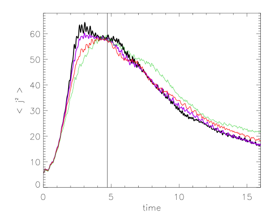
Figure 1: Current density, $<J^{2}>$, as function of time for $\epsilon=0$, $1/32$, $1/16$ and $1/8$. The color of these curves are, black, violet, red and green respectively (color online). The thickness of the lines decreases proportionally to the value of $\epsilon$, thus, the thicker line corresponds to $\epsilon=0$ and the finest line to $\epsilon=1/8$. The vertical straight line indicates a particular time where all the scales have been developed in all runs. Besides, in this time the value of $<J^{2}>$ is approximately the same for all runs. This particular time will be used to study the different structures in the flows.

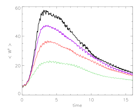
Figure 2: Vorticity, $<\omega^{2}>$, as function of time for $\epsilon=0$, $1/32$, $1/16$ and $1/8$. We are using the same convention of color/thickness than in figure 1

Figure 3 shows $<J^{2}+\omega^{2}>$ as function of time, the difference between the peaks is more clear in this case. Here we see two effects that occur simultaneously as the Hall coefficient is increased: The decrease in the dissipation and the delay in reaching the maximum point (and hence the time that it takes to develop all the scales). The first effect will have a direct impact on the dissipation scale of the respective flows while the second shows how the Hall term modifies its characteristic times.

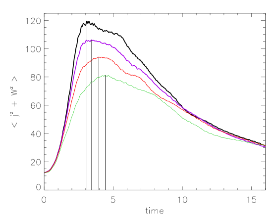
Figure 3: $<J^{2}+\omega^{2}>$ as function of time for $\epsilon=0$, $1/32$, $1/16$ and $1/8$. We are using the same convention of color/thickness than in figure 1. The vertical straight lines indicate the maximum value for each curve.

It is relevant to note that the dissipation scale ($1/K_{diss}$) is related to the number of scales that develop in the flow. It is common to consider that the decrease in the dissipation scale increases the range of developed scales in the flow (usually increases the size of the inertial range). In the same manner, the increase in the scale of dissipation leads to a decrease in the number of scales developed in the flow. However, it is not always this case. The results that we will show below indicate that the Hall term affects the total width of the dissipation range decreasing mildly the $K_{diss}$ (and therefore mildly increasing the dissipation scale) with the increase of the $\epsilon$, at the same time the delays suffered by the dissipation peaks is due to the development of a greater number of scales in the dissipative range due to a major accumulation of energy in these scales.

To quantify the dissipation scale (in Fourier space) of the different flows we use the conventional criteria bisk given by the equation (17).

$$K_{diss}=\left(\frac{<\bm{\omega}^{2}>+<\bm{J}^{2}>}{\nu^{2}}\right)^{1/4}$$ (17)

In Table 1 the Hall scale is shown along with the dissipation scale for each one of the flows. Here we see the decrease of the $K_{diss}$ in quantitative form with the increase of the Hall coefficient. Note that $K_{diss}<K_{max}=N/3=170$ means that the runs are marginally resolved (see Wan et al 2010 wan for more demanding requirements if higher order statistic is performed)

Table 1: Hall and dissipation scales for the different runs.

Run	$\epsilon$	$K_{Hall}$	$K_{diss}$
1	0		132.25
2	1/32	32	125.40
3	1/16	16	124.58
4	1/8	8	120.08

The decrease of the global dissipation with the Hall parameter and the increase in the time of the peak development can not be understood by looking only at the temporal evolution of the global magnitudes. These effects could be due to a change in the characteristic time of the energy flow or to the development of small scale structures.

To better understand these issues we study the energy spectra and the size and shape of the structures generated in the four runs. This help us to see whether or not the Hall effect produces the development of small scales and also to understand this dynamic in terms of the energy distribution.

Looking at the spectra we can see the distribution of the energy through different scales. Figure 4 compares the energy spectra for all runs and Figure 5 shows a zoom around of the Hall scales used.

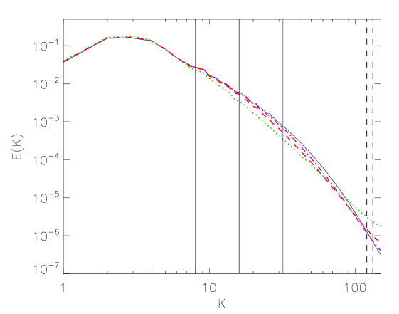
Figure 4: Energy spectra for $\epsilon=0$ (solid line), $\epsilon=1/32$ (dash-dotted), $\epsilon=1/16$ (dash) and $\epsilon=1/8$ (dotted). The vertical straight lines indicate the differents values of $K_{Hall}=1/\epsilon$ for $\epsilon=1/32,1/16,1/8$. The vertical straight dashed lines show the minimun and the maximum values of the $K_{diss}$ ($\epsilon=1/8$ and $\epsilon=0$), through them we can see the effect of the Hall term on the dissipation scale.

As the Hall parameter is increased the energy spectrum is steeper at intermediate scales preceeding the dissipation range. At the same time there is an increase in the energy on scales smaller (larger $k$) than the dissipation scale (see Figs. 4 and 5). The effect of the Hall term is then twofold: first there is a slow down of the energy transfer up to the Hall scale, resulting in a steeper spectrum, and then there seems to be a driving of energy from the Hall scale up to the small scales (see Min3 for a study of how the Hall term affects the transfer of energy at different scales). A shift of the effective dissipation scale to larger scales is then to be expected (as indicated by the values of $K_{diss}$ given before) as well as a decrease in the global dissipation values. At the same time, since the Hall term increases the number of effective scales on which the dynamics occurs (as evindenced by the extended spectra at small scales) a longer time to reach the peak of dissipation is expected, as previously shown.

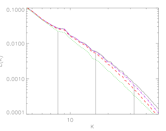
Figure 5: Enlarged view of a section of the energy spectra (limited $k$). The vertical straight lines indicate the different values of $K_{Hall}=1/\epsilon$ for $\epsilon=1/32,1/16,1/8$, these lines intersect each of the corresponding curves.

We study the characteristic structures of the flow and the effect of the Hall term by looking at the current density field. Figures 6-9 show the parallel component of the current density in a perpendicular plane to the external magnetic field at a given time for the different runs. The time was chosen in which all scales have been developed for all the flows (this time is indicated in Figure 1). Also, for this particular time, the value of $<J^{2}>$ is approximately the same for all the runs.

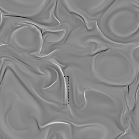
Figure 6: Parallel component of the current density in a perpendicular plane to the external magnetic field in the case with $\epsilon=0$ .Tones indicate out of plane current, with light tones=positive and dark tones=negative.

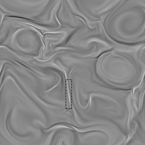
Figure 7: Parallel component of the current density in a perpendicular plane to the external magnetic field in the case with $\epsilon=1/32$ .Tones indicate out of plane current, with light tones=positive and dark tones=negative.

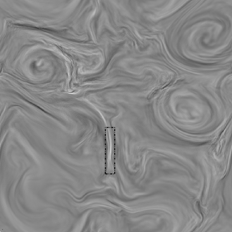
Figure 8: Parallel component of the current density in a perpendicular plane to the external magnetic field in the case with $\epsilon=1/16$ .Tones indicate out of plane current, with light tones=positive and dark tones=negative.

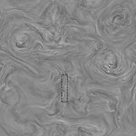
Figure 9: Parallel component of the current density in a perpendicular plane to the external magnetic field in the case with $\epsilon=1/8$ .Tones indicate out of plane current, with light tones=positive and dark tones=negative.

In Figure 6 ($\epsilon=0$) we can clearly distinguish the current sheets that form in the flow. We have highlighted one of the current sheets with a rectangle with dashed lines. This structure is localized and well defined. Looking at the change of this structure with the value of Hall parameter we can see two effects: first, a widening of the sheet and secondly an internal filamentation. The widening is very clear from Figure 6 with $\epsilon=0$ to Figure 7 with $\epsilon=1/32$ and the internal filamentation starts to be seen in the Figure 8, with $\epsilon=1/16$, where also the thickness has increased. In the case with higher $\epsilon=1/8$ the current sheet is completely filamentated, and is hard to distinguish a clear structure at all.

These results are complementary to the results observed in the spectra and global magnitudes and corroborate the idea that the Hall effect results in an effective shift of the dissipation scale (current sheet thickness getting larger) but also an increase in the dynamical scale range (increase of filamentation).

To better quantify the effect we have just observed, we plot the profile of the current density in the direction perpendicular to the current sheet seen in the figures 6-9. These profiles are shown in Figure 10.

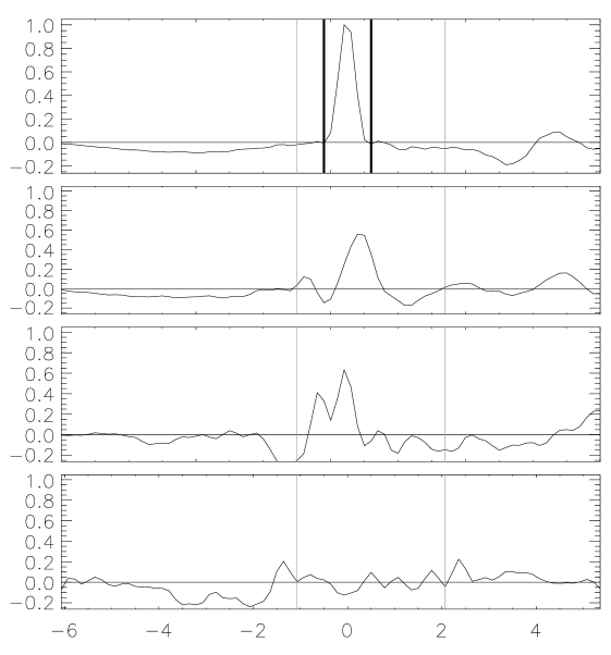
Figure 10: Current density profile of the current sheets studied. From top to bottom are the cases with $\epsilon=0$, $\epsilon=1/32$, $\epsilon=1/16$, and $\epsilon=1/8$. The net flow of current (the absolute value) is the same within the clear lines (vertical outside lines), and the dark lines mark the original position of the current sheet when $\epsilon=0$.

The net flow of current (the absolute value) is the same within the clear lines (vertical outside lines). When $\epsilon=0$ the current sheet is perfectly located (the dark lines mark the original position of the current sheet when $\epsilon=0$) and it is homogeneous (in the sense that we have a single well defined peak). When $\epsilon=1/32$ the original sheet expands and two sheets or filaments appear in their place (there are now two peaks). For $\epsilon=1/16$ the width of the main sheet is greater and there is now a clear internal structure. In this case the ambiguity that arises is whether we have one or more sheets of current (compare Figure 10 with 8) and hence the ambiguity of whether we have a wider sheet or two thin sheets. When $\epsilon=1/8$ there is no trace of the current sheet.

At this point we should make an important observation about the evolution of current sheets as a function of the Hall parameter. As we saw there are two effects acting simultaneously, the widening of what could be considered the overall structure of the sheet and the internal filamentation that this suffers. In this way it could be interpreted that the Hall effect widens the current sheets (if we see the entire structure like the sheet) or on the other hand the Hall effect produces finer sheets (considering that the small filaments are the sheets). To remove the ambiguity (in semantics), we propose to speak in terms of dissipation, so if the global structure dissipates less energy as we increase the Hall parameter we will say that the sheet is being widened, otherwise, if more energy is dissipated we will say that the relation between size and intensity of internal filaments allow us to identify new current sheets. Our results agree with the first frame of mind: as a function of dissipation the current sheets are widening and even more when $\epsilon=1/8$ there is no trace of any structure that could be identified as a current sheet.

IV Conclusions

We performed numerical simulations of magnetohydrodynamic turbulence in strong magnetic fields, including the Hall effect, and varying the Hall parameter.

We found that the Hall term affects the scales that are situated between the Hall scale and the dissipation scale, resulting in a decrease in the accumulation of energy in this scale range. The result is an effective shift of the dissipation scale but also a transfer of energy to smaller scales. When the separation between the Hall scale and the dissipation scale is larger an increasingly sharp steepening of the energy spectrum occurs at this range of scales. The final outcome is the generation of smaller scales when the Hall scale increases.

Localized structures are destroyed by this effect, suffering a gradual filamentation with the increase of the Hall scale. The latter effect is manifested, for example, in the widening of the current sheets and the formation of internal structures within the sheets. At the same time a decrease of the total energy dissipated is observed.

The results presented here suggest that the Hall effect reduces the intermittency, however a more detailed study of this property should be performed. We defer this to further work.

- (1) N. A. Krall and A. W. Trivelpiece, in Principles of Plasma Physics (McGraw-Hill, New York, 1973), p. 89.
- (2) L. Turner, IEEE Trans. Plasma Sci. PS14, 849 (1986).
- (3) J. Birn, J. F. Drake, M. A. Shay et al., J. Geophys. Res. 106, 3715 (2001).
- (4) X. Wang, A. Bhattacharjee, and Z. W. Ma, Phys. Rev. Lett. 87, 265003 (2001).
- (5) F. Mozer, S. Bale, and T. D. Phan, Phys. Rev. Letter. 89, 015002 (2002).
- (6) D. Smith, S. Ghosh, P. Dmitruk, and W. H. Matthaeus. Geophys. Res Lett. 31, L02805 (2004).
- (7) L. F. Morales, S. Dasso, and D. O. Gomez, J. Geophys. Res. 110, A04204 (2005).
- (8) P. D. Mininni, D. O. Gomez, and S. M. Mahajan, Astrophys. J. 584, 1120 (2003).
- (9) M. Wardle, Mon. Not. R. Astron. Soc. 303, 239 (1999).
- (10) S. A. Balbus and C. Terquem, Astrophys. J. 552, 235 (2001).
- (11) W. H. Matthaeus, P. Dmitruk, D. Smith, S. Ghosh, and S. Oughton, Geophys. Res. Lett. 30, 2104 (2003).
- (12) P. D. Mininni, D. O. Gomez, and S. M. Mahajan, Astrophys. J. 619, 1019 (2005).
- (13) S. Galtier, J. Plasma Phys. 72, 721 (2006).
- (14) P. Dmitruk and W. H. Matthaeus, Phys. Plasmas 13, 042307 (2006).
- (15) L. N. Martin, P. Dmitruk, Phys. Plasma 17, 112304 (2010).
- (16) D. O. Gomez, S. M. Mahajan, and P. Dmitruk, Phys. Plasma 15, 102303 (2008).
- (17) N. H. Bian and D. Tsiklauri, Phys. Plasma 16, 064503 (2009).
- (18) G. P. Zank and W. H. Matthaeus, J. Plasma Phys. 48, 85 (1992).
- (19) A. A. van Ballegooijen, Astrophys. J. 311, 1001 (1986).
- (20) D. W. Longcope, and R. N. Sudan, Astrophys. J. 437, 491 (1994).
- (21) D. L. Hendrix and G. van Hoven, Astrophys. J. 467, 887 (1996).
- (22) L. Milano, P. Dmitruk, C. H. Mandrini, D. O. Gómez, and P. Demoulin, Astrophys. J. 521, 889 (1999).
- (23) D. O. Gómez, and C. Ferro Fontán, Astrophys. J. 394, 662 (1992).
- (24) P. Dmitruk and D. O. Gómez, Astrophys. J. Lett. 527, L63 (1999).
- (25) P. Dmitruk, D. O. Gómez, and W. H. Matthaeus, Phys. Plasmas 10, 3584 (2003).
- (26) S. Oughton, P. Dmitruk, and W. H. Matthaeus, Phys. Plasmas 11, 2214 (2004).
- (27) P. Dmitruk, W. H. Matthaeus, and S. Oughton, Phys. Plasmas 12, 112304 (2005).
- (28) S. Ghosh, m. Hossain, and W. H. Matthaeus, Comput: Phys. Commun. 74, 18 (1993).
- (29) D. Biskamp, Magnetohydrodynamic Turbulence (Cambridge University Press, Cambridge, England, 2003).
- (30) P. D. Mininni, A. Alexakis, and A. Pouquet, J. Plasma Phys.
- (31) M. Wan, S. Oughton, S. Servidio, and W. H. Matthaeus, Phys. Plasma 17, 082308 (2010). 73, 377 (2007).