General Analysis Tool Box for
Controlled Perturbation

Abstract

The implementation of reliable and efficient geometric algorithms is a challenging task. The reason is the following conflict: On the one hand, computing with rounded arithmetic may question the reliability of programs while, on the other hand, computing with exact arithmetic may be too expensive and hence inefficient. One solution is the implementation of controlled perturbation algorithms which combine the speed of floating-point arithmetic with a protection mechanism that guarantees reliability, nonetheless.

This paper is concerned with the performance analysis of controlled perturbation algorithms in theory. We answer this question with the presentation of a general analysis tool box for controlled perturbation algorithms. This tool box is separated into independent components which are presented individually with their interfaces. This way, the tool box supports alternative approaches for the derivation of the most crucial bounds. We present three approaches for this task. Furthermore, we have thoroughly reworked the concept of controlled perturbation in order to include rational function based predicates into the theory; polynomial based predicates are included anyway. Even more we introduce object-preserving perturbations. Moreover, the tool box is designed such that it reflects the actual behavior of the controlled perturbation algorithm at hand without any simplifying assumptions.

1 Introduction

1.1 Robust Geometric Computing

It is a notoriously difficult task to cope with rounding errors in computing [22, 13]. In computational geometry, predicates are decided on the sign of mathematical expressions. If rounding errors cause a wrong decision of the predicate, geometric algorithms may fail in various ways: inconsistency of the data (e.g., contradictory topology), loops that do not terminate or loops that terminate unexpectedly [38]. In addition, the thoughtful processing of degenerate cases makes the implementation of geometric algorithms laborious [4]. The meaning of degeneracy always depends on the context (e.g., three points on a line, four points on a circle). There are several ways to overcome the numerical robustness issues and to deal with degenerate inputs.

The exact computation paradigm [36, 37, 43, 23, 58, 44] suggests an implementation of an exact arithmetic. This is established by a number representation of variable precision (i.e., variable bit length) or the use of symbolic values which are not evaluated (e.g., roots of integers). There are several implementations of such number types [10, 42, 49, 48, 44]. Each program must be developed carefully such that it can deal with all possible degenerate cases. The software libraries Leda and Cgal follow the exact computation paradigm [44, 39, 18]. The paradigm was also taken as a basis in [3, 53, 27].

As opposed to that, the topology oriented approach [54, 34, 55] is based on an arithmetic of finite precision. To avoid numerical robustness issues, the main guideline is the maintenance of the topology. This objective requires individual alterations of the algorithm at hand and it seems that it cannot be turned into an easy-to-use general framework. Furthermore, this approach must also cope with degenerate inputs. However, the speed of floating-point arithmetic may be worth the trouble; in addition with other accelerations, Held [31] has implemented a very fast computation of the Voronoi diagram of line segments.

There are also problem-oriented solutions. In computational geometry, the sign of determinants decides an interesting class of predicates. For example, the side-of-line or the in-circle predicate in the plane belong to this class and are used in the computation of Delaunay diagrams. Some publications attack the numerical issues in the evaluation of determinants directly [2, 5].

The previous approaches have in common that they primarily focus on the numerical issues. Other approaches are originated from the degeneracy issue. A slight perturbation of the input seems to solve this problem. There are different approaches which are based on perturbation. The symbolic perturbation, see for example [14, 57, 56, 15, 16, 52, 47], provides a general way to distort inputs such that degeneracies do not occur. This definitely provides a shorter route for the presentation of geometric algorithms. Practically this approach requires exact arithmetic to avoid robustness issues. Therefore the pitfall in this approach is that, if the concept requires very small perturbations, it implicates a high precision and possibly a slow implementation.

In this paper we focus on controlled perturbation. This variant was introduced by Halperin et al. [30] for the computation of spherical arrangements. There a perturbed input is a random point in the neighborhood of the initial input. It is unlikely, but not impossible, that the input is degenerate. Therefore the algorithm has a repeating perturbation process with two objectives: Finding an input that does not contain degeneracies and that leads to numerically robust floating-point evaluations. Halperin et al. have presented mechanisms to respond to inappropriate perturbations. Moreover, they have argued formally under which conditions there is a chance for a successful termination of their algorithm. Controlled perturbation leads to numerically robust implementations of algorithms which use non-exact arithmetic and which do not need to process degenerate cases.

This idea of controlled perturbation was applied to further geometric problems afterwards: The arrangement of polyhedral surfaces [29], the arrangement of circles  [28], Voronoi diagrams and Delaunay triangulations [40, 25]. However, the presentation of each specific algorithm has required a specific analysis of its performance. This broaches the subject of a general method to analyze controlled perturbation algorithms.

We remark that controlled perturbation has also a shady side: Although it solves the problem for the perturbed input exactly, it does not solve it for the initial input. Furthermore, it is non-obvious how to receive a solution for the initial input in general. In case the input is highly degenerated, the running time of the algorithm may increase significantly after the permutation [8, 1]. In this case, the specialized treatment of degeneracies may be much faster.

1.2 Our contribution

The study of a general method to analyze controlled perturbation algorithms is a joint work with Kurt Mehlhorn and Michael Sagraloff. We have firstly presented the idea in [45]. Then Caroli [9] studied the applicability of the method for predicates which are used for the computation of arrangements of circles (according to [28]) and the computation of Voronoi diagrams of line segments (according to [6, 51]). Our significantly improved journal article contains, furthermore, a detailed discussion of the analysis of multivariate polynomials [46].

Independent of former publications, the author has redeveloped the topic from scratch to design a sophisticated tool box for the analysis of controlled perturbation algorithms. The tool box is valid for floating-point arithmetic, guides step by step through the analysis and allows alternative components. Furthermore, the solutions of two open problems are integrated into the theory. We briefly present our achievements below.

We present a general tool box to analyze algorithms and their predicates. The tool box is subdivided into independent components and their interfaces. Step-by-step instructions for the analysis are associated with each component. Interfaces represent bounds that are used in the analysis. The result is a precision function or a probability function. Furthermore, necessary conditions for the analysis are derived from the interfaces (e.g., the notion of criticality differs from former publications).

We present alternative approaches to derive necessary bounds. Because we have subdivided the tool box into independent components and their interfaces, it is possible to make alternative components available in the most crucial step of the analysis. The direct approach is based on the geometric meaning of predicates, the bottom-up approach is based on the composition of functions, and the top-down approach is a coordinate-wise analysis of functions. Similar direct and top-down approaches are presented in [45, 46]. This is the first time that a bottom-up approach is presented for this task.

The result of the analysis is valid for floating-point arithmetic. A random floating-point number generator that guarantees a uniform distribution was introduced in [46]. But, so far, the result of the analysis was never proven to be valid for the finite set of floating-point numbers since the Lebesgue measure cannot take sets of measure zero into account. To overcome this issue, we define a specialized perturbation generator and pay attention to the finiteness in the analysis, namely, in the success probability, in the (non-)exclusion of points and in the usage of the Lebesgue measure.

We present an alternative analysis of multivariate polynomials. An analysis of multivariate polynomials, which resembles the top-down approach, is presented in [46]. Here we present an alternative analysis which makes use of the bottom-up approach.

We solve the open problem of analyzing rational functions. We include poles of rational functions into the theory and describe the treatment of floating-point range errors in the analysis. We suggest a general way to guard rational functions in practice and we show how to analyze the behavior of these guards in theory.

We solve the open problem of object-preserving perturbations. We introduce a perturbation generator that makes it possible to perturb the location of input objects without deforming the objects itself. To achieve this goal, we have designed the perturbation such that the relative floating-point input specifications of the objects are preserved despite of the usage of rounded arithmetic.

We suggest an implementation that is in accordance with the analysis tool box. We define a fixed-precision perturbation generator and extend it to be object-preserving. We explain the particularities in the practical treatment of range errors that occur especially in the case of rational functions. Finally, we show how to realize guards for rational functions.

1.3 Content

In this paper we present a tool box for a general analysis of controlled perturbation algorithms. In Section 2, we present the basic design principles of controlled perturbation from a practical point of view. Fundamental quantities and definitions of the analysis are introduced in Section 3. The general analysis tool box and all of its components are briefly introduced in Section 4. Its detailed presentation is structured in two parts: The function analysis and the algorithm analysis.

Geometric algorithms base their decisions on geometric predicates which are decided by signs of real-valued functions. Therefore the analysis of algorithms requires a general analysis of such functions. The function analysis is visualized in Figure 7 on Page 7. Since the analysis is performed with real arithmetic, we must also prove its validation for actual floating-point inputs. This validation is anchored in Section 5. The function analysis itself works in two stages. The required bounds form the interface between the stages and are presented in Section 6. The method of quantified relations represents the actual analysis in the second stage and is introduced in Section 7. The derivation of the bounds in the first stage uses the direct approach of Section 8, the bottom-up approach of Section 9, or the top-down approach of Section 10, together with an error analysis which is introduced in Section 11. In Section 12 we extend the analysis and the implementation such that both properly deal with floating-point range errors. As examples, we present the analysis of multivariate polynomials in Section 9 and the analysis of rational functions in Section 13.

The algorithm analysis is visualized in Figure 25 on Page 25. The algorithm analysis works also in two stages. In the first stage, we perform the function analyses and derive some algorithm specific bounds. The analysis itself in the second stage is represented by the method of distributed probability. The algorithm analysis is entirely presented in Section 14.

Furthermore, we present a general way to implement controlled perturbation algorithms in Section 15 such that our analysis tool box can be applied to them. Even more, we suggest a way to implement object-preserving perturbations in Section 16.

A quick reference to the most important definitions of this paper can be found in the appendix in Section 17.

2 Controlled Perturbation Algorithms

This section contains an introduction to the basic principles for controlled perturbation algorithms. We have already mentioned that implementations of geometric algorithms must address degeneracy issues and numerical robustness issues. We review floating-point arithmetic in Section 2.1 and present the basic design principles of controlled perturbation algorithms in Section 2.2.

2.1 Floating-point Arithmetic

Variable precision arithmetic is necessary for a general implementation of controlled perturbation algorithms. We explain this statement with the following thought experiment that can be skipped during first reading: Assume we compute an arrangement of $n$ circles incrementally with a fixed precision arithmetic. Let us further assume that there is an upper bound on the radius of the circles. Then, because of the fixed precision, the number of distinguishable intersections per circle must be limited. Hence the computation of a dense arrangement gets stuck after a certain amount of insertions unless we allow circles to be moved (perturbed) further away from their initial location. Asymptotically, this policy transforms a very dense arrangement into an arrangement of almost uniformly distributed circles. Therefore we demand that the precision of the arithmetic can be chosen arbitrarily large.

A floating-point number is given by a sign, a mantissa, a radix and a signed exponent. In the regular case, its value is defined as

value $$:= \text{sign}\cdot\text{mantissa}\cdot\text{radix}^{\text{exponent}}.$$

Without loss of generality, we assume the radix to be 2. The bit length of the mantissa is called precision $L$. We denote the bit length of the exponent by $K$. The discrete set of regular floating-point numbers is a subset of the rational numbers. Furthermore, this set is finite for fixed $L$ and $K$.

A floating-point arithmetic defines the number representation (the radix, $L$ and $K$), the operations, the rounding policy and the exception handling for floating-point numbers (see Goldberg [26]). A technical standard for fixed precision floating-point arithmetic is IEEE 754-2008 (see [33]). Nowadays, the built-in types single, double and quadruple precision are usual for radix 2.

There are several software libraries that offer variable precision floating-point arithmetic. Cgal provides the multi-precision floating-point number type MP_Float (see the Cgal manual [10]). Core provides the variable precision floating-point number type CORE::BigFloat (see [42]). And Leda provides the variable precision floating-point number type leda_bigfloat (see the Leda book [44]). Be aware that the rounding policy and exception handling of certain libraries may differ from the IEEE standard. Since our analysis partially presumes this standard, we must ensure that the arithmetic in use is appropriate. The Gnu Multiple Precision Floating-Point Reliable Library, for example, “provides the four rounding modes from the IEEE 754-1985 standard, plus away-from-zero, as well as for basic operations as for other mathematical functions” (see the Gnu Mpfr manual [49]). Moreover, Gnu Mpfr is used for the multiple precision interval arithmetic which is provided by the Multiple Precision Floating-point Interval library (see the Gnu Mpfi manual [48]).

Variable precision arithmetic is more expensive than built-in fixed precision arithmetic. We remark that, in practice, we try to solve the problem at hand with built-in arithmetic first and, in addition, try to make use of floating-point filters. Throughout the paper we use the following notations.

Definition 1 (floating-point)

Let $L,K\in\mathbb{N}$. By ${\mathbb{F}_{L,K}}$ we denote:
1. The set of floating-point numbers with radix 2, precision $L$ and $K$-bit exponent.
2. The floating-point arithmetic that is induced by the set characterized in 1.
Furthermore, we define the suffix $\!|_{\mathbb{F}}$ for sets and expressions:
1. Let $k\in\mathbb{N}$ and let $X\subset\mathbb{R}^{k}$. Then $X\!|_{\mathbb{F}}:=X\cap\mathbb{F}^{k}$.
2. $f(x)\!|_{\mathbb{F}}$ denotes the floating-point value of $f(x)$ evaluated with arithmetic $\mathbb{F}$.

That means, by $X\!|_{\mathbb{F}}$ we denote the restriction of $X$ to its subset that can be represented with floating-point numbers in $\mathbb{F}$. To simplify the notation we omit the indices $L$ or $K$ of ${\mathbb{F}_{L,K}}$ whenever they are given by the context. For the same reason we have already skipped the dimension $k$ in the suffix $\!|_{\mathbb{F}}$.

2.2 Basic Controlled Perturbation Implementations

Rounding errors of floating-point arithmetic may influence the result of predicate evaluations. Wrong predicate evaluations may cause erroneous results of the algorithm and even lead to non-robust implementations (see Kettner et al. [38]). In order to get correct and robust implementations, we introduce guards which testify the reliability of predicate evaluations (see [24, 7, 46]).

Definition 2 (guard)

Let $\mathbb{F}$ be a floating-point arithmetic and let $f:X\to\mathbb{R}$ be a function with $X\subset\mathbb{R}^{k}$. We call a predicate ${\cal G}_{f}:X\to\text{\{true, false\}}$ a guard for $f\!$ on $X$ if

$${\cal G}_{f}(x) \Rightarrow \quad\text{\rm sign}(f(x)\!|_{\mathbb{F}})=\text{\rm sign}(f(x))$$ is true

for all $x\in X\!|_{\mathbb{F}}$. Presumed that there is such a predicate ${\cal G}_{f}$, we say that an input $x\in X\!|_{\mathbb{F}}$ is guarded if ${\cal G}_{f}(x)$ is true and unguarded if ${\cal G}_{f}(x)$ is false.

That means, guards testify the sign of function evaluations. A design of guards is presented in Section 11. By means of guards we can implement geometric algorithms such that they can either verify or disprove their result.

Definition 3 (guarded algorithm)

We call an algorithm ${\cal A}_{\text{\rm G}}$ a guarded algorithm if there is a guard for each predicate evaluation and if the algorithm halts either with the correct combinatorial result or with the information that a guard has failed. If ${\cal A}_{\text{\rm G}}$ halts with the correct result, we also say that ${\cal A}_{\text{\rm G}}$ is successful, and we say that ${\cal A}_{\text{\rm G}}$ has failed if a guard has failed.

Let $\bar{y}$ be an input of ${\cal A}_{\text{\rm G}}$. In case ${\cal A}_{\text{\rm G}}(\bar{y})$ is successful, we obtain the desired result for input $\bar{y}$. Of course, the situation is unsatisfying if ${\cal A}_{\text{\rm G}}$ fails. Therefore we introduce controlled perturbation (see Halperin et al. [28]): We execute ${\cal A}_{\text{\rm G}}$ for randomly perturbed inputs $y$ (i.e., random points in the neighborhood of $\bar{y}$) until ${\cal A}_{\text{\rm G}}$ terminates successfully. Furthermore, we increase the precision $L$ of the floating-point arithmetic $\mathbb{F}$ after each failure in the hope to improve the chance to succeed. (It is the task of the analysis to give evidence.) We summarize this idea in the provisional controlled perturbation algorithm $\text{\rm basic-}{\cal A}_{\text{\rm CP}}$ which is shown in Algorithm 1. The general controlled perturbation algorithm is presented on page 2 in Section 14.

Algorithm 1 : $\text{\rm basic-}{\cal A}_{\text{\rm CP}}({\cal A}_{\text{\rm G}},\bar{y},{\cal U}_{\delta})$

  /* initialization */

  $L\leftarrow$ precision of built-in floating-point arithmetic

  repeat

     /* run guarded algorithm */

     $y\leftarrow$ random point in ${\overline{\cal U}}_{\delta}(\bar{y})\!|_{\mathbb{F}_{L}}$

     $\omega\leftarrow{\cal A}_{\text{\rm G}}(y,{\mathbb{F}_{L}})$

     /* adjust parameters */

     if ${\cal A}_{\text{\rm G}}$ failed then

        $L\leftarrow 2L$

     end if

  until ${\cal A}_{\text{\rm G}}$ succeeded

  /* return perturbed input $y$ and result $\omega$ */

  return  $(y,\omega)$

We see that there is an implementation of $\text{\rm basic-}{\cal A}_{\text{\rm CP}}({\cal A}_{\text{\rm G}})$ for every guarded algorithm ${\cal A}_{\text{\rm G}}$, or to say it in other words, for every algorithm that is only based on geometric predicates that can be guarded. It is important to note that this does not necessarily imply that $\text{\rm basic-}{\cal A}_{\text{\rm CP}}$ performs well. It is the main objective of this paper to develop a general method to analyze the performance of controlled perturbation algorithms ${\cal A}_{\text{\rm CP}}$.

3 Fundamental Quantities and Definitions

Our main aim is the derivation of a general method to analyze controlled perturbation algorithms. In order to achieve this, we introduce fundamental quantities first. In Section 3.1 we define the quantities that describe the situation which we want to analyze. We encounter and discuss many issues during the definition of the success probability in Section 3.2. This is the first presentation of a detailed modelling of the floating-point success probability. Controlled perturbation specific quantities are introduced in Section 3.3. (Further analysis specific bounds are defined in the presentation of the analysis later on.) The overview in Section 3.4 summarizes the classification of inputs in practice and in the analysis. In Section 3.5 we present conditions under which we may apply controlled perturbation to a predicate in practice and under which we can actually justify its application in theory.

3.1 Perturbation, Predicate, Function

Here we define the quantities that are needed to describe the initial situation: the original input, the perturbation area, the perturbation parameter, the perturbed input, the input value bound, functions that realize geometric predicates, and predicate descriptions.

In the analysis we assume that the original input $\bar{y}$ of a controlled-perturbation algorithm ${\cal A}_{\text{\rm CP}}$ consists of $n$ floating-point numbers, that means, $\bar{y}\in\mathbb{F}^{n}$ or, as we prefer to say, $\bar{y}\in\mathbb{R}^{n}\!|_{\mathbb{F}}$. At this point we do not care for a geometrical interpretation of the input of ${\cal A}_{\text{\rm CP}}$. We remark that this is no restriction: a complex number can be represented by two numbers; a vector can be represented by the sequence of its components; geometric objects can be represented by their coordinates and measures; and so on. A circle in the plain, for example, can be represented by a 6-tuple (the coordinates of three distinct points in the circle) or a 3-tuple (the coordinates of the center and the radius). And, to carry the example on, an input of $m$ circles can be interpreted as a tuple $\bar{y}\in\mathbb{R}^{n}\!|_{\mathbb{F}}$ with $n:=6m$ if we choose the first variant.

We define the perturbation of $\bar{y}$ as a random additive distortion of its components. We call ${\cal U}_{\delta}(\bar{y})\subset\mathbb{R}^{n}$ a perturbation area with perturbation parameter $\delta$ if

1. $\delta\in\mathbb{R}_{>0}^{n}$,
2. $y\in{\cal U}_{\delta}(\bar{y})$ implies $|y_{i}-\bar{y}_{i}|\leq\delta_{i}$ for $1\leq i\leq n$ and
3. ${\cal U}_{\delta}(\bar{y})$ contains an (open) neighborhood of $\bar{y}$.

Note that ${\cal U}_{\delta}(\bar{y})$ is not a discrete set whereas ${\cal U}_{\delta}(\bar{y})\!|_{\mathbb{F}}$ is finite. In our example, if we allow a circular perturbation of the $3m$ points which define the $m$ input circles, the perturbation area is the Cartesian product of $3m$ planar discs. We make the observation that even if we consider the input as a plain sequence of numbers, the perturbation area may look very special—we cannot neglect the geometrical interpretation here! In this context, we define an axis-parallel perturbation area $U_{\delta}(\bar{y})$ as a box which is centered in $\bar{y}$ and has edge length $2\delta_{i}$ parallel to the $i$-th main axis (and always denote it by the latin letter $U$ instead of ${\cal U}$). This definition significantly simplifies the shape of the perturbation area.

Naturally, the perturbed input must also be a vector of floating-point numbers. For now, we denote the perturbed input by $y\in{\cal U}(\bar{y})\!|_{\mathbb{F}}$. (We remark that we refine this definition on page 3).

The analysis of ${\cal A}_{\text{\rm CP}}$ depends on the analysis of ${\cal A}_{\text{\rm G}}$ and its predicates (see Section 14). We remember that a geometric predicate, which is true or false, is decided by the sign of a real-valued function $f$. Therefore we introduce further quantities to describe such functions. We assume that $f$ is a $k$-ary real-valued function and that $k\ll n$. We further assume that we evaluate $f$ at $k$ distinct perturbed input values, that means, we evaluate $f(y_{\sigma(1)},\ldots,y_{\sigma(k)})$ where $\sigma:\{1,\ldots,k\}\to\{1,\ldots,n\}$ is injective. The mapping $\sigma$ is injective to guarantee that the variables in the formula of $f$ are independent of each other. To not get the indices mixed up in the analysis, we rename the argument list of $f$ into $x_{i}:=y_{\sigma(i)}$ for $1\leq i\leq k$. In the same way we also rename the affected input values $\bar{x}_{i}:=\bar{y}_{\sigma(i)}$. We denote the set of valid arguments for $f$ by $A$.

In the analysis, ${e_{\text{\rm max}}}$ implicitly describes an upper-bound on the absolute value of perturbed input values in the way

$${e_{\text{\rm max}}} := \min\left\{e^{\prime}\in\mathbb{N}\,:\,\text{$|\bar{y}_{i}|+\delta_{i}\leq 2^{e^{\prime}}$ for all $1\leq i\leq n$}\right\}.$$ (1)

We call ${e_{\text{\rm max}}}$ the input value parameter. Be aware that this is just a bound on the arguments of $f$ and not a bound on the absolute value of $f$. At the moment we assume that the absolute value of $f$ is bounded on $A$ and that the size $K$ of the exponent of the floating-point arithmetic ${\mathbb{F}_{L,K}}$ is sufficiently large to avoid overflow errors during the evaluation of $f$. In Section 12, we drop this assumption and discuss the treatment of range issues.

Below we summarize the basic quantities which are needed for the analysis of a function $f$.

Definition 4

We call ${(f,k,A,\delta,{e_{\text{\rm max}}})}$ a predicate description if:

1. $k\in\mathbb{N}$,
2. $A\subset\mathbb{R}^{k}$,
3. $\delta\in\mathbb{R}_{>0}^{k}$,
4. ${e_{\text{\rm max}}}$ is as it is defined in Formula (1),
5. $\bar{U}_{\delta}(A)\subset[-2^{{e_{\text{\rm max}}}},2^{{e_{\text{\rm max}}}}]^{k}$ and
6. $f:\bar{U}_{\delta}(A)\to\mathbb{R}$.

Predicate descriptions are used on and on. We extend the notion in Definition 9 on page 9 and in Definition 12 on page 12.

3.2 Success Probability, Grid Points

The controlled-perturbation algorithm ${\cal A}_{\text{\rm CP}}$ terminates eventually if there is a positive probability that ${\cal A}_{\text{\rm G}}$ terminates successfully. The latter condition is fulfilled if $f$ has the property: The probability of a successful evaluation of $f$ gets arbitrarily close to the certain event just by increasing the precision $L$. We call this property applicability and specify it in Section 3.5.

In this section we derive a definition for the success probability that is appropriate for the analysis and that is valid for floating-point evaluations. We begin with the question: What is the least probability that a guarded evaluation of $f$ is successful in a run of ${\cal A}_{\text{\rm G}}$ under the arithmetic $\mathbb{F}$? We assume that each random point is chosen with the same probability. Then the answer is

$$\text{\rm pr}(f\!|_{\mathbb{F}}) := \min_{\bar{x}\in A}\;\frac{{\left|\,\left\{x\in\bar{U}_{\delta}(\bar{x})\!|_{\mathbb{F}}\,:\,\text{${\cal G}(x)$ is true}\right\}\,\right|}}{{\left|\,\bar{U}_{\delta}(\bar{x})\!|_{\mathbb{F}}\,\right|}}.$$

The definition really reflects the actual behavior of $f$. The probability is the number of guarded (floating-point) inputs divided by the total number of inputs and considers the worst-case for all perturbation areas.

Issue 1: Floating-point arithmetic is hard to be analyzed directly

Because floating-point arithmetic and its rounding policy can hardly be analyzed directly, we aim at deriving a corresponding formula for real arithmetic. In real space, we use the Lebesgue measure $\mu$ to determine the volume of areas. Therefore we are looking for a formula like

$$\text{\rm pr}(\text{$f$}) := \min_{\bar{x}\in A}\;\frac{\mu\left(\left\{x\in\bar{U}_{\delta}(\bar{x})\,:\,\text{${\cal G}^{\prime}(x)$ is true}\right\}\right)}{\mu({\bar{U}_{\delta}(\bar{x})})}$$ (2)

where the predicate ${\cal G}^{\prime}:\bar{U}_{\delta}(A)\to\text{\{true, false\}}$ equals ${\cal G}$ at arguments with floating-point representation.

Issue 2: The set of floating-point numbers has measure zero

It is well-known that the set $\bar{U}_{\delta}(\bar{x})\!|_{\mathbb{F}}$ is finite and that its superset $\bar{U}_{\delta}(\bar{x})\!|_{\mathbb{Q}}$ is a set of measure zero. Be aware that the fraction in Formula (2) does not change if we redefine $f$ on a set of measure zero. This implies some bizarre situations. For example, let ${f_{\text{false}}}:\bar{U}_{\delta}(A)\to\mathbb{R}$ be

$${f_{\text{false}}}(x) := \left\{\begin{array}[]{r@{\quad:\quad}l}f(x)&x\not\in\bar{U}_{\delta}(A)\!|_{\mathbb{Q}}\\ 0&otherwise\end{array}\right.$$

and let ${f_{\text{true}}}:\bar{U}_{\delta}(A)\to\mathbb{R}$ be

$${f_{\text{true}}}(x) := \left\{\begin{array}[]{r@{\quad:\quad}l}f(x)&x\not\in\bar{U}_{\delta}(A)\!|_{\mathbb{Q}}\\ B&otherwise\end{array}\right.$$

where $B\in\mathbb{R}_{>0}$ is large enough to guarantee that the guard ${\cal G}$ evaluates to true in the latter case. Be aware that $\text{\rm pr}(\text{${f_{\text{false}}}$})=\text{\rm pr}(\text{${f_{\text{true}}}$})$ due to Formula (2) whereas both implementations “${\cal A}_{\text{\rm G}}$ with ${f_{\text{true}}}$” and “${\cal A}_{\text{\rm G}}$ with ${f_{\text{false}}}$” behave most conflictive: The former is always successful whereas the latter never succeeds. We remark that the assumption “$f$ is (upper) continuous almost everywhere” does not solve the issue because “almost everywhere” means “with the exception of a set of measure zero.” We have to introduce several restrictions to get able to deal with situations like that.

Issue 3: There is no general relation between $\text{\rm pr}(f\!|_{\mathbb{F}})$ and $\text{\rm pr}(f)$

This problem gets already visible in the 1-dimensional case.

Example 1

Let $\mathbb{F}=\mathbb{F}_{2,3}$ be the floating-point arithmetic with $L=2$ and $K=3$. In addition let $U=[0,2]$, $R_{1}=[0,1]$ and $R_{2}=[1,2]$ be intervals. The situation is depicted in Figure 1.

Figure 1: Distribution of the discrete set $\mathbb{F}_{2,3}$ within the interval $[0,2]$.

What is the probability that a randomly chosen point $x\in U$ lies inside of $R_{1}$, respectively $R_{2}$, for points in $U$ or $U\!|_{\mathbb{F}}$? Note that $R_{1}$ and $R_{2}$ have the same length. For $R_{1}=[0,1]$ we have

$$\text{\rm pr}(R_{1})=\frac{1}{2}\quad{<}\quad\text{\rm pr}(R_{1}\!|_{\mathbb{F}})=\frac{17}{21},$$

that means, the probability is higher for floating-point arithmetic. On the other hand, for $R_{2}=[1,2]$ we have

$$\text{\rm pr}(R_{2})=\frac{1}{2}\quad{>}\quad\text{\rm pr}(R_{2}\!|_{\mathbb{F}})=\frac{5}{21},$$

that means, the probability is higher for real arithmetic. $\bigcirc$

We derive from Example 1 that there is no general relation between $\text{\rm pr}(f\!|_{\mathbb{F}})$ and $\text{\rm pr}(f)$ because of the distribution of $\mathbb{F}$.

Issue 4: Distribution of $\mathbb{F}$ is non-uniform

Because the discrete set of floating-point numbers is non-uniformly distributed in general, we smartly alter the perturbation policy: We restrict the random choice of floating-point numbers to selected numbers that lie on a regular grid.

Definition 5 (grid)

Let ${e_{\text{\rm max}}}$ be as it is defined in Formula (1) and let ${\mathbb{F}_{L,K}}$ be a floating-point arithmetic (with ${e_{\text{\rm max}}}\ll 2^{K-1}$). We define

$$\tau := 2^{{e_{\text{\rm max}}}-L-1}.$$ (5)

We call

$${\mathbb{G}_{L,K,{e_{\text{\rm max}}}}} := \left\{\lambda\tau\,:\,\text{$\lambda\in\mathbb{Z}$ and $\lambda\tau\in[-2^{e_{\text{\rm max}}},2^{e_{\text{\rm max}}}]$}\right\}$$ (6)

the grid points induced by ${e_{\text{\rm max}}}$ with respect to ${\mathbb{F}_{L,K}}$ and we call $\tau$ the grid unit of ${\mathbb{G}_{L,K,{e_{\text{\rm max}}}}}$. Furthermore, we denote the grid points $\mathbb{G}$ inside of a set $X\subset\mathbb{R}^{k}$ by

$$X\!|_{\mathbb{G}} := X\cap\mathbb{G}^{k}.$$

Again we omit the indices whenever they do not deserve special attention. We observe that the grid unit $\tau$ is the maximum distance between two adjacent points in $\mathbb{F}\cap[-2^{e_{\text{\rm max}}},2^{e_{\text{\rm max}}}]$. We observe further that the grid points $\mathbb{G}$ form a subset of $\mathbb{F}$. Be aware that the symbol $\mathbb{F}$ represents a set or an arithmetic whereas the symbol $\mathbb{G}$ always represents a set. It is important to see that the underlying arithmetic is still $\mathbb{F}$. We have introduced $\mathbb{G}$ only to change the definition of the original perturbation area into ${\overline{\cal U}}_{\delta}(\bar{y})\!|_{\mathbb{G}}$. This leads to the final version of the success probability of $f$: The least probability that a guarded evaluation of $f$ is successful for inputs in $\mathbb{G}$ under the arithmetic $\mathbb{F}$ is

$$\text{\rm pr}(f\!|_{\mathbb{G}}) := \min_{\bar{x}\in A}\;\frac{{\left|\,\left\{x\in\bar{U}_{\delta}(\bar{x})\!|_{\mathbb{G}}\,:\,\text{${\cal G}(x)$ is true}\right\}\,\right|}}{{\left|\,\bar{U}_{\delta}(\bar{x})\!|_{\mathbb{G}}\,\right|}}.$$ (7)

Before we continue this consideration, we add a remark on the implementation of the perturbation area ${\overline{\cal U}}_{\delta}(\bar{y})\!|_{\mathbb{G}}$.

Remark 1

Because the points in $\mathbb{G}$ are uniformly distributed, the implementation of the perturbation is significantly simplified to the random choice of integer $\lambda$ in Formula (6). This functionality is made available by basically all higher programming languages. Apart from that we generate floating-point numbers with the largest possible number of trailing zeros. This possibly reduces the rounding error in practice.

Issue 5: Projection of ${\overline{\cal U}}_{\delta}(\bar{y})\!|_{\mathbb{G}}$ is non-uniform

The original perturbation area ${\overline{\cal U}}_{\delta}(\bar{y})\!|_{\mathbb{G}}$ is a discrete set of uniformly distributed points of which every point is chosen with the same probability. As a consequence, the predicate perturbation area $\bar{U}_{\delta}(\bar{x})\!|_{\mathbb{G}}$ is also uniformly distributed. But it is important to see that this does not imply that all points in the projected grid appear with the same probability! We illustrate, explain and solve this issue in Section 14. For now we continue our consideration under the assumption that all points in $\bar{U}_{\delta}(\bar{x})\!|_{\mathbb{G}}$ are uniformly distributed and randomly chosen with the same probability.

Issue 6: Analyses for various perturbation areas may differ

In the determination of $\text{\rm pr}(f\!|_{\mathbb{G}})$ in Formula (7), we encounter the difficulty to find the minimum ratio between the guarded and all possible inputs for all possible perturbation areas, that means, for all $\bar{x}\in A$. We can address this problem with a simple worst-case consideration if we cannot gain (or do not want to gain) further insight into the behavior of $f$: We just expect that, whatever could negatively affect the analysis of $f$ within the total predicate perturbation area $\bar{U}_{\delta}(A)$, affects the perturbation area $\bar{U}_{\delta}(\bar{x})$ under consideration. This way, we safely obtain a lower bound on the minimum.

Issue 7: There is no general relation between $\text{\rm pr}(f\!|_{\mathbb{G}})$ and $\text{\rm pr}(f)$

Example 2

We continue Example 1. In addition let $R_{3}=[\frac{1}{10},\frac{9}{10}]$ be an interval. Because $U\subseteq[-2^{1},2^{1}]$, we have ${e_{\text{\rm max}}}=1$ and $\tau=2^{{e_{\text{\rm max}}}-L-1}=\frac{1}{4}$. The situation is depicted in Figure 2.

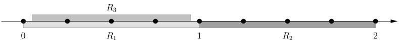
Figure 2: The distribution of the grid points $\mathbb{G}_{2,3,1}$ within the interval $[0,2]$.

Again we compare the continuous and the discrete case: What is the probability that a randomly chosen point $x\in U$ lies inside of $R_{1}$ ($R_{2}$ or $R_{3}$, respectively)? The probability is now higher for $R_{1}$ and $R_{2}$ in the discrete case

$$\text{\rm pr}(R_{1})=\text{\rm pr}(R_{2})=\frac{1}{2}\quad<\quad\text{\rm pr}(R_{1}\!|_{\mathbb{G}})=\text{\rm pr}(R_{2}\!|_{\mathbb{G}})=\frac{5}{9},$$

and higher for $R_{3}$

$$\text{\rm pr}(R_{3})=\frac{2}{5}\quad>\quad\text{\rm pr}(R_{3}\!|_{\mathbb{G}})=\frac{1}{3}$$

in the real case. $\bigcirc$

We make the observation that the restriction to points in $\mathbb{G}$ does not entirely solve the initial problem: We still cannot relate the probability $\text{\rm pr}(f)$ with $\text{\rm pr}(f\!|_{\mathbb{G}})$ in general. To improve the estimate, we need another trick that we indicate in Example 3: If we make the interval slightly larger, we can safely determine the inequality.

Example 3

Let $\tau$ be the grid unit of $\mathbb{G}$. We define three intervals $R\subset R_{\text{\rm aug}}\subset U$. Let $U\subset\mathbb{R}$ be a closed interval of length $\lambda_{0}\tau$ with $\lambda_{0}\in\mathbb{N}$. Let $R_{\text{\rm aug}}\subset U$ be an interval of length at least $\tau$ that has the limits $R_{\text{\rm aug}}:=[a-\frac{\tau}{2},b+\frac{\tau}{2}]$ for $a,b\in\mathbb{R}$. Finally, we define $R:=[a,b]$. In addition let $\lambda\in\mathbb{N}$ be such that

$$\lambda\tau\;\;\leq\;\;\mu(R_{\text{\rm aug}})\;\;<\;\;(\lambda+1)\tau.$$

We observe that the number of grid points in $R\!|_{\mathbb{G}}$ and $R_{\text{\rm aug}}\!|_{\mathbb{G}}$ is bounded by

$$\lambda-1\;\;\leq\;\;{\left|\,R\!|_{\mathbb{G}}\,\right|}\;\;\leq\;\;\lambda\;\;\leq\;\;{\left|\,R_{\text{\rm aug}}\!|_{\mathbb{G}}\,\right|}\;\;\leq\;\;\lambda+1.$$

Moreover, we make the important observation that

$$\frac{{\left|\,R\!|_{\mathbb{G}}\,\right|}}{{\left|\,U\!|_{\mathbb{G}}\,\right|}}\;\;\leq\;\;\frac{\lambda}{\lambda_{0}+1}\;\;\leq\;\;\frac{\lambda}{\lambda_{0}}\;\;=\;\;\frac{\lambda\tau}{\lambda_{0}\tau}\;\;\leq\;\;\frac{\mu(R_{\text{\rm aug}})}{\mu(U)}.$$

That means, it is more likely that a random point in $U$ lies inside of $R_{\text{\rm aug}}$ than a random point in $U\!|_{\mathbb{G}}$ lies inside of $R\!|_{\mathbb{G}}$. The inequality

$$\text{\rm pr}(R\!|_{\mathbb{G}}) \leq \text{\rm pr}(R_{\text{\rm aug}})$$

is valid independently of the actual choice or location of $R$. $\bigcirc$

Issue 8: There is still no general relation between $\text{\rm pr}(f\!|_{\mathbb{G}})$ and $\text{\rm pr}(f)$

The probability $\text{\rm pr}(f)$ is defined as the ratio of volumes. The definition is, in particular, independent of the location and shape of the involved sets. As an example, we consider the three different (shaded) regions in Figure 3 which all have the same volume.

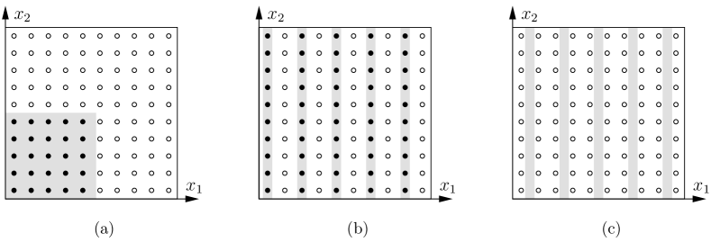
Figure 3: The volume of the shaded region $R$ is the same in the three pictures. Depending on the shape and location of $R$, it covers various fractions of the discrete set $\mathbb{G}$. For example: (a) a quarter, (b) a half, (c) nothing.

We make the important observation that the shape and location matter if we derive the induced ratio for points in $\mathbb{G}$. The discrepancy between the ratios is caused by the implicit assumption that the grid unit $\tau$ is sufficiently small. (Asymptotically, the ratios approach the same limit in the three illustrated examples for $\tau\to 0$.) Be aware that making this assumption explicit leads to a second constraint on the precision $L$ which we call the grid unit condition. To solve this issue, we need a way to adjust the grid unit $\tau$ to the shape of $R$. We address this issue in general in Section 5.1. For now we continue our consideration under the assumption that this problem is solved.

Summary and validation of $\text{\rm pr}(f\!|_{\mathbb{G}})$

We summarize our considerations so far. The analysis of a guarded algorithm must reflect its actual behavior. (What would be the meaning of the analysis, otherwise?) Therefore we have defined the success probability of a floating-point evaluation of $f$ in Formula (7) such that it is based on the behavior of guards. Furthermore, we have studied the interrelationship between the success probability for floating-point and real arithmetic to prepare the analysis in real space. Be aware that we have introduced a specialized perturbation on a regular grid $\mathbb{G}$ (in practice and in analysis) which is necessary for the derivation of the interrelationship. Moreover, we now make this relationship explicit for a single interval. (The general relationship is formulated in Section 5.1.)

Example 4

(Continuation of Example 3.) Let $f:U\to\mathbb{R}$. We assume the following property of $R$: If $x\in U\!|_{\mathbb{G}}$ lies outside of $R$ then the guard ${\cal G}(x)$ is true. Then we have

$$\text{\rm pr}(f\!|_{\mathbb{G}}) = \frac{{\left|\,\left\{x\in U\!|_{\mathbb{G}}\,:\,\text{${\cal G}(x)$ is true}\right\}\,\right|}}{{\left|\,U\!|_{\mathbb{G}}\,\right|}}$$

$$\geq 1\,-\,\frac{{\left|\,R\!|_{\mathbb{G}}\,\right|}}{{\left|\,U\!|_{\mathbb{G}}\,\right|}}$$

$$\geq 1\,-\,\frac{\mu(R_{\text{\rm aug}})}{\mu(U)}.$$

We conclude: If we prove by means of abstract mathematics that

$$1\,-\,\frac{\mu(R_{\text{\rm aug}})}{\mu(U)} \geq p$$

for a probability $p\in(0,1)$, we have implicitly proven that

$$\text{\rm pr}(f\!|_{\mathbb{G}}) \geq p$$

for a randomly chosen grid point in $\mathbb{G}$. Be aware that $\text{\rm pr}(f\!|_{\mathbb{G}})$ is defined only by discrete quantities. $\bigcirc$

Warning: processing exceptional points

We explain in this paragraph why it is absolutely non-obvious how to process exceptional points in general. Assume that we want to exclude the set $D\subset A$ from the analysis. This changes our success probability from Formula (7) into

$$\text{\rm pr}(f\!|_{\mathbb{G}}) = \min_{\bar{x}\in A}\;\frac{{\left|\,\left\{x\in\bar{U}_{\delta}(\bar{x})\!|_{\mathbb{G}}\,:\,\text{${\cal G}(x)$ is true}\right\}\setminus D\,\right|}}{{\left|\,\bar{U}_{\delta}(\bar{x})\!|_{\mathbb{G}}\,\right|}}$$

$$\geq \min_{\bar{x}\in A}\;\frac{\max\left\{0,\;{\left|\left\{x\in\bar{U}_{\delta}(\bar{x})\!|_{\mathbb{G}}\,:\,\text{${\cal G}(x)$ is true}\right\}\right|}-{|D|}\right\}}{{\left|\,\bar{U}_{\delta}(\bar{x})\!|_{\mathbb{G}}\,\right|}}.$$

To obtain a practicable solution, it is reasonable to assume that $D$ is finite and, moreover, that $|D|\ll{\left|\,\bar{U}_{\delta}(\bar{x})\!|_{\mathbb{G}}\,\right|}$. This changes the relation in Example 4 into:

$$\text{\rm pr}(f\!|_{\mathbb{G}}) \geq \max\left\{0,\;1-\frac{\mu(R_{\text{\rm aug}})}{\mu(U)}-\frac{|D|}{{\left|\,\bar{U}_{\delta}(\bar{x})\!|_{\mathbb{G}}\,\right|}}\right\}.$$

It is important to see that this estimate still contains two quantities that depend on the floating-point arithmetic. But our plan was to get rid of this dependency. In spite of the simplifying assumptions it is non-obvious how to perform the analysis in real space in general. Our suggested solution to this issue is to avoid exceptional points. Alternatively we declare them critical (see next section) which triggers an exclusion of their environment.

3.3 Fp-safety Bound, Critical Set, Region of Uncertainty

The fp-safety bound

We introduce a predicate that can certify the correct sign of floating-point evaluations. The essential part of this predicate is the fp-safety bound. We show in Section 11 that there are fp-safety bounds for a wide class of functions.

Definition 6 (lower fp-safety bound)

Let ${(f,k,A,\delta,{e_{\text{\rm max}}})}$ be a predicate description. Let $S_{\inf f}:\mathbb{N}\to\mathbb{R}_{\geq 0}$ be a monotonically decreasing function that maps a precision $L$ to a non-negative value. We call $S_{\inf f}$ a (lower) fp-safety bound for $f\!$ on $A$ if the statement

$$|f(x)|>S_{\inf f}(L)\quad \Rightarrow \quad\text{\rm sign}(f(x)\!|_{\mathbb{F}_{L}})=\text{\rm sign}(f(x))$$ (8)

is true for every precision $L\in\mathbb{N}$ and for all $x\in\bar{U}_{\delta}(A)\!|_{\mathbb{F}_{L}}$.

For the time being, we consider $K$ to be a constant. We drop this assumption in Section 12 where we introduce upper fp-safety bounds. Until then we only consider lower fp-safety bounds.

The critical set

Next we introduce a classification of the points in $\bar{U}_{\delta}(A)$ in dependence on their neighborhood. (We refine the definition on Page 20.)

Definition 7 (critical)

Let ${(f,k,A,\delta,{e_{\text{\rm max}}})}$ be a predicate description. We call a point $c\in\bar{U}_{\delta}(\bar{x})$ critical if

$$\inf_{x\in U_{\varepsilon}(c)\setminus\{c\}}\;\left|f(x)\right| = 0$$ (9)

on a neighborhood $U_{\varepsilon}(c)$ for infinitesimal small $\varepsilon>0$. Furthermore, we call zeros of $f$ that are not critical less-critical. Points that are neither critical nor less-critical are called non-critical. We define the critical set $C_{f,\delta}$ of $f$ at $\bar{x}\in A$ with respect to $\delta$ as the union of critical and less-critical points within $\bar{U}_{\delta}(\bar{x})$.

In other words, we call $c$ critical if there is a Cauchy sequence $(a_{i})_{i\in\mathbb{N}}$ in $\bar{U}_{\delta}(\bar{x})\setminus\{c\}$ where $\lim_{i\to\infty}a_{i}=c$ and $\lim_{i\to\infty}f(a_{i})=0$. We remember that the metric space $\mathbb{R}^{k}$ is complete, that means, the limit of the sequence $(a_{i})$ lies inside of the closure $\bar{U}_{\delta}(\bar{x})$. Sometimes we omit the indices of the critical set $C$ if they are given by the context.

Example 5

We consider the three functions that are depicted in Figure (4). Let $f_{1}(x)=x^{2}$. Let $f_{2}(x)=x^{2}$ for $x\neq 0$ and $f_{2}(0)=2$. Let $f_{3}(x)=x^{2}+1$ for $x\not\in\{-2,1\}$ and $f_{3}(-2)=0$ and $f_{3}(1)=0.2$.

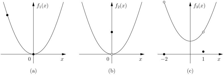
Figure 4: Examples of critical, less-critical and non-critical points.

The point $x=0$ in Picture (a) is a zero and a critical point for $f_{1}$. In (a), every argument $x\neq 0$ is non-critical for $f_{1}$. In (b), $f_{2}$ is non-zero at $x=0$, but $x=0$ is a critical point for $f_{2}$. In (c), the argument $x=-2$ is less-critical for $f_{3}$ and the argument $x=1$ is non-critical for $f_{3}$. $\bigcirc$

What is the difference of critical and less-critical points? We observe that the point $c$ is excluded from its neighborhood in Formula (9). Zeros of $f$ would trivially be critical otherwise. Furthermore, we observe that zeros of continuous functions are always critical. For our purpose it is important to see that the infimum of $|f|$ is positive if we exclude the less-critical points itself and neighborhoods of critical points. Be aware that we technically could treat both kinds differently in the analysis and still ensure that the result of the analysis is valid for floating-point arithmetic. Only for simplicity we deal with them in the same way by adding these points to the critical set. Only for simplicity we also add exceptional points to the critical set.

The region of uncertainty

The next construction is a certain environment of the critical set.

Definition 8 (region of uncertainty)

Let ${(f,k,A,\delta,{e_{\text{\rm max}}})}$ be a predicate description. In addition let $\gamma\in\mathbb{R}_{>0}^{k}$. We call

$$R_{f,\gamma}(\bar{x}) := \bar{U}_{\delta}(\bar{x})\;\cap\;\left(\bigcup_{c\in C_{f,\delta}(\bar{x})}U_{\gamma}(c)\right)$$ (10)

the region of uncertainty for $f$ induced by $\gamma$ with respect to $\bar{x}$.

In our presentation we use the axis-parallel boxes $U_{\gamma}(c)$ to define the specific $\gamma$-neighborhood of $C$; other shapes require adjustments, see Section 5.1. The sets $U_{\gamma}(c)$ are open and the complement of $R_{f,\gamma}(\bar{x})$ in $\bar{U}_{\delta}(\bar{x})$ is closed. We omit the indices of the region of uncertainty $R$ if they are given by the context.

The vector $\gamma$ defines the tuple of componentwise distances to $c$. The presentation requires a formal definition of the set of all admissible $\gamma$. This set is either a box or a line. Let $\hat{\gamma}\in\mathbb{R}_{>0}^{k}$. Then we define the unique open axis-parallel box with vertices $0$ and $\hat{\gamma}$ as

$${\Gamma\text{\rm-box\,}_{\hat{\gamma}}} := \left\{\gamma^{\prime}=(\gamma^{\prime}_{1},\ldots,\gamma^{\prime}_{k}):\text{$\gamma^{\prime}_{i}\in(0,\hat{\gamma}_{i})$ for all $i\in I$}\right\}$$

and the open diagonal from 0 to $\hat{\gamma}$ inside of ${\Gamma\text{\rm-box\,}_{\hat{\gamma}}}$ as

$${\Gamma\text{\rm-line\,}_{\hat{\gamma}}} := \left\{\gamma:\text{$\gamma=\lambda\hat{\gamma}$ with $\lambda\in(0,1)$}\right\}.$$

It is important that the $\gamma_{i}$ can be chosen arbitrarily small whereas the upper bounds $\hat{\gamma}_{i}$ are only introduced for technical reasons; we assume that $\hat{\gamma}$ is “sufficiently” small. Occasionally we omit $\hat{\gamma}$.

We have already seen that there is need to augment the region of uncertainty (see Issue 7 and 8 in Section 3.2). This task is accomplished by the mapping $\gamma\mapsto{\text{\rm aug}}(\gamma):=\frac{\gamma}{t}$ for $t\in(0,1)$. For technical reasons we remark that $\gamma\in{\Gamma\text{\rm-box\,}_{\hat{\gamma}}}$ if ${\text{\rm aug}}(\gamma)\in{\Gamma\text{\rm-box\,}_{\hat{\gamma}}}$, and $\gamma\in{\Gamma\text{\rm-line\,}_{\hat{\gamma}}}$ if ${\text{\rm aug}}(\gamma)\in{\Gamma\text{\rm-line\,}_{\hat{\gamma}}}$. We call $R_{f,{\text{\rm aug}}(\gamma)}$ the augmented region of uncertainty for $f$ under ${\text{\rm aug}}(\gamma)$. By $\Gamma$ we denote the set of valid augmented $\gamma$ and include it in the predicate description.

Definition 9

We extend Definition 4 and call ${(f,k,A,\delta,{e_{\text{\rm max}}},\Gamma)}$ a predicate description if: 7. $\Gamma={\Gamma\text{\rm-line\,}_{\hat{\gamma}}}$ or $\Gamma={\Gamma\text{\rm-box\,}_{\hat{\gamma}}}$ for a sufficiently small $\hat{\gamma}\in\mathbb{R}_{>0}^{k}$.

3.4 Overview: Classification of the Input

In practice and in the analysis we deal with real-valued functions whose signs decide predicates. The arguments of these functions belong to the perturbation area. In this section we give an overview of the various characteristics for function arguments that we have introduced so far. We strictly distinguish between terms of practice and terms of the analysis.

The diagram of the practice-oriented terms is shown in Figure 5. We consider the discrete perturbation area $U_{\!\delta}\,\!|_{\mathbb{G}}$. Controlled perturbation algorithms ${\cal A}_{\text{\rm CP}}$ are designed with intent to avoid the implementation of degenerate cases and to compute the combinatorial correct solution. Therefore the guards in the embedded algorithm ${\cal A}_{\text{\rm G}}$ must fail for the zero set and for arguments whose evaluations lead to wrong signs. The guard is designed such that the evaluation is definitely fp-safe if the guard does not fail (light shaded region). Unfortunately there is no convenient way to count (or bound) the number of arguments in $U_{\!\delta}\,\!|_{\mathbb{G}}$ for which the guard fails. That is the reason why we perform the analysis with real arithmetic and introduce further terms.

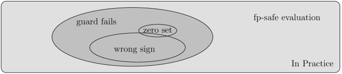
Figure 5: The diagram of the practice-oriented terms.

The diagram of the analysis-oriented terms is shown in Figure 6. We consider the real perturbation area $U_{\!\delta}$. Instead of the zero set, we consider the critical set (see Definition 7). The critical set is a superset of the zero set. Then we choose the region of uncertainty as a neighborhood of the critical set (see Definition 8). We augment the region of uncertainty to obtain a result that is also valid for floating-point evaluations. We intent to prove fp-safety outside of the augmented region of uncertainty (i.e. on the light shaded region). Therefore we design a fp-safety bound that is true outside of the region. This way we can guarantee that the evaluation of a guard (in practice) only fails on a subset of the augmented region (in the analysis).

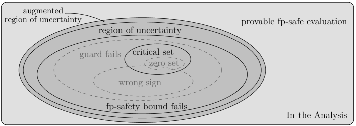
Figure 6: The diagram of the analysis-oriented terms (shown in black).

3.5 Applicability and Verifiability of Functions

We study the circumstances under which we may apply controlled perturbation to a predicate in practice and under which we can actually verify its application in theory. We stress that we talk about a qualitative analysis here; the desired quantitative analysis is derived in the following sections.

Furthermore, we want to remark that verifiability is not necessary for the presentation of the analysis tool box. However, the distinction between applicability, verifiability and analyzability was important for the author during the development of the topic. We keep it in the presentation because it may also be helpful to the reader. Anyway, skipping this section is possible and even assuming equality between verifiability and analyzability will do no harm.

In practice

We specify the function property that the probability of a successful evaluation of $f$ gets arbitrarily close to the certain event by increasing the precision.

Definition 10 (applicable)

Let ${(f,k,A,\delta,{e_{\text{\rm max}}})}$ be a predicate description. We call $f$ applicable if for every $p\in(0,1)$ there is $L_{p}\in\mathbb{N}$ such that the guarded evaluation of $f$ is successful at a randomly perturbed input $x\in\bar{U}_{\delta}(\bar{x})\!|_{\mathbb{G}_{L}}$ with probability at least $p$ for every precision $L\in\mathbb{N}$ with $L\geq L_{p}$ and every $\bar{x}\in A$.

Applicable functions can safely be used in guarded algorithms: Since the precision $L$ is increased (without limit) after a predicate has failed, the success probability gets arbitrarily close to 1 for each predicate evaluation. As a consequence, the success probability of ${\cal A}_{\text{\rm G}}$ gets arbitrarily close to 1, too.

In the qualitative analysis

Unfortunately we cannot check directly if $f$ is applicable. Therefore we introduce two properties that imply applicability.

Definition 11

Let ${(f,k,A,\delta,{e_{\text{\rm max}}},{\Gamma\text{\rm-line}},t)}$ be a predicate description.

• (region-condition). For every $p\in(0,1)$ there is $\gamma\in\mathbb{R}_{>0}^{k}$ such that the geometric failure probability is bounded in the way

  $$\frac{\mu(R_{\gamma}(\bar{x}))}{\mu(U_{\delta}(\bar{x}))} \leq (1-p)$$ (11)

  for all $\bar{x}\in A$. We call this condition the region-condition.

• (safety-condition). There is a fp-safety bound $S_{\inf f}:\mathbb{N}\to\mathbb{R}_{>0}$ on $\bar{U}_{\delta}(A)$ with

  $$\lim_{L\to\infty}S_{\inf f}(L) = 0.$$ (12)

  We call this condition the safety-condition.

• (verifiable). We call $f$ verifiable on $\bar{U}_{\delta}(A)$ for controlled perturbation if $f$ fulfills the region- and safety-condition.

The region-condition guarantees the adjustability of the volume of the region of uncertainty. Note that the region-condition is actually a condition on the critical set. It states that the critical set is sufficiently “sparse”.

The safety-condition guarantees the adjustability of the fp-safety bound. It states that for every $\varphi>0$ there is a precision ${L_{\text{\rm safe}}}\in\mathbb{N}$ with the property that

$$S_{\inf f}(L)\leq\varphi$$ (13)

for all $L\in\mathbb{N}$ with $L\geq{L_{\text{\rm safe}}}$. We give an example of a verifiable function.

Example 6

Let $A\subset\mathbb{R}$ be an interval, let $\delta\in\mathbb{R}_{>0}$ and let $f:\bar{U}_{\delta}(A)\to\mathbb{R}$ be a univariate polynomial of degree $d$ with real coefficients, i.e.,

$$f(x) = a_{d}\cdot x^{d}+a_{d-1}\cdot x^{d-1}+\ldots+a_{1}\cdot x+a_{0}.$$

We show that $f$ is verifiable. Part 1 (region-condition). Because of the fundamental theorem of algebra (e.g., see Lamprecht [41]), $f$ has at most $d$ real roots. Therefore the size of the critical set $C_{f}$ is bounded by $d$ and the volume of the region of uncertainty $R_{\gamma}(\bar{x})$ is upper-bounded by $2d\gamma$. For a given $p\in(0,1)$ we then choose

$$\gamma := \frac{(1-p)\delta}{d}$$

which fulfills the region-condition because of

$$\frac{\mu(R_{\gamma}(\bar{x}))}{\mu(U_{\delta}(\bar{x}))} \leq \frac{2\gamma d}{2\delta}\;\;=\;\;1-p.$$

Part 2 (safety-condition). Corollary 3 on page 3 provides the fp-safety bound

$$S_{\inf f}(L) := (d+2)\,\max_{1\leq i\leq d}|a_{i}|\;\,2^{{e_{\text{\rm max}}}(d+1)+1-L}$$

for univariate polynomials. Since $S_{\inf f}(L)$ converges to zero as $L$ approaches infinity, the safety-condition is fulfilled. Therefore $f$ is verifiable. $\bigcirc$

We show that, if a function is verifiable, it has a positive lower bound on its absolute value outside of its region of uncertainty.

Lemma 1

Let ${(f,k,A,\delta,{e_{\text{\rm max}}},{\Gamma\text{\rm-line}},t)}$ be a predicate description and let $f$ be verifiable. Then for every $\gamma\in\mathbb{R}_{>0}^{k}$, there is $\varphi\in\mathbb{R}_{>0}$ with

$$\varphi\leq|f(x)|$$ (14)

for all $x\in\bar{U}_{\delta}(\bar{x})\setminus R_{\gamma}(\bar{x})$ and for all $\bar{x}\in A$.

Proof

We assume the opposite. That means, in particular, for every $i\in\mathbb{N}$ there is $a_{i}\in\bar{U}_{\delta}(\bar{x})\setminus R_{\gamma}(\bar{x})$ such that $|f(a_{i})|<\frac{1}{i}$. Then $(a_{i})_{i\in\mathbb{N}}$ is a bounded sequence with accumulation points in $\bar{U}_{\delta}(\bar{x})\setminus R_{\gamma}(\bar{x})$. Those points must be critical and hence belong to $R_{\gamma}(\bar{x})$. This is a contradiction. ∎

Finally we prove that verifiability of functions implies applicability.

Lemma 2

Let ${(f,k,A,\delta,{e_{\text{\rm max}}},{\Gamma\text{\rm-line}},t)}$ be a predicate description and let $f$ be verifiable. Then $f$ is applicable.

Proof

Let $p\in(0,1)$. Then the geometric success probability is bounded by $p$. Therefore there must be an upper bound on the volume of the region of uncertainty (see Definition 11). In addition there is a precision ${L_{\text{\rm grid}}}$ such that we may interpret this region as an augmented region $R_{{\text{\rm aug}}(\gamma)}$ (see Theorem 5.1). Furthermore, there must be a positive lower bound on $|f|$ outside of $R_{\gamma}$ (see Lemma 1). Moreover, there must be a precision ${L_{\text{\rm safe}}}$ for which the fp-safety bound is smaller than the bound on $|f|$. Be aware that this implies that the guarded evaluation of $f$ is successful at a randomly perturbed input with probability at least $p$ for every precision $L\geq\max\{{L_{\text{\rm safe}}},{L_{\text{\rm grid}}}\}$. That means, $f$ is applicable (see Definition 10). ∎

4 General Analysis Tool Box

The general analysis tool box to analyze controlled perturbation algorithms is presented in the remainder of the paper. We call the presentation a tool box because its components are strictly separated from each other and sometimes allow alternative derivations. In particular, we present three ways to analyze functions. Here we briefly introduce the tool box and refer to the detailed presentation of its components in the subsequent sections. The decomposition of the analysis into well-separated components and their precise description is an innovation of this presentation.

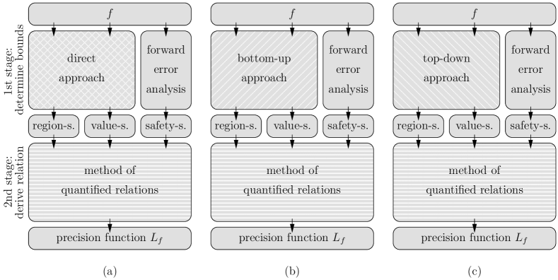
Figure 7: Illustration of the various ways to analyze functions.

The tool box is subdivided into components. At first we explain the analysis of functions. The diagram in Figure 7 illustrates three ways to analyze functions. We subdivide the function analysis in two stages. The analysis itself in the second stage requires three necessary bounds, also known as the interface, which are defined in Section 6: region-suitability, value-suitability and safety-suitability. In Section 7 we introduce the method of quantified relations which represents the actual analysis in the second stage. In the first stage, we pay special attention to the derivation of two bounds of the interface and suggest three different ways to solve the task. We show in Section 8 how the bounds can be derived in a direct approach from geometric measures. Furthermore, we show how to build-up the bounds for the desired function from simpler functions in a bottom-up approach in Section 9. Moreover, we present a derivation of the bounds by means of a “sequence of bounds” in a top-down approach in Section 10. Finally, we show how we can derive the third necessary bound of the interface with an error analysis in Section 11

We deal with the analysis of algorithms in Section 14. The idea is illustrated in Figure 25 on page 25. Again we subdivide the analysis in two stages. The actual analysis of algorithms is the method of distributed probability which represents the second stage and is explained in Section 14.3. The interface between the stages is subdivided in two groups. Firstly, there are algorithm prerequisites (to the left of the dashed line in the figure). These bounds are defined and derived in Section 14.1: evaluation-suitability, predicate-suitability and perturbation-suitability. Secondly, there are predicate prerequisites (to the right of the dashed line in the figure). These are determined by means of function analyses.

5 Justification of Analyses in Real Space

This section addresses the problem to derive the success probability for floating-point evaluations from the success probability which we determine in real space. Analyses in real space are without meaning for controlled perturbation implementations (which use floating-point arithmetic), unless we determine a reliable relation between floating-point and real arithmetic. To achieve this goal, we introduce an additional constraint on the precision in Section 5.1 and summarize our efforts in the determination of the success probability in Section 5.2. This is the first presentation that adjusts the precision of the floating-point arithmetic to the shape of the region of uncertainty.

5.1 The Grid Unit Condition

Here we adjust the distance of grid points (i.e., the grid unit $\tau$) to the “width” of the region of uncertainty $\gamma$. As we have seen in Issue 8 in Section 3.2, the grid unit $\tau$ must be sufficiently small (i.e., $L$ must be sufficiently large) to derive a reliable probability $\text{\rm pr}(f\!|_{\mathbb{G}})$ from $\text{\rm pr}(f)$. The problem is illustrated in Figure 3 on page 3. We call this additional constraint on $L$ the grid unit condition

$$L \geq {L_{\text{\rm grid}}}$$ (15)

for a certain ${L_{\text{\rm grid}}}\in\mathbb{N}$. Informally, we demand that $\tau\ll\gamma$. Here we show how to derive the threshold ${L_{\text{\rm grid}}}$ formally. We refine the concept of the augmented region of uncertainty which we have mentioned briefly in Section 3.2. The discussion of Issue 7 suggests an additive augmentation $\gamma={\text{\rm aug}}(\gamma^{\prime})$ that fulfills

$$\tau_{0} \stackrel{{\scriptstyle(I)}}{{\leq}} \gamma^{\prime}_{i}\;\;\stackrel{{\scriptstyle(II)}}{{\leq}}\;\;\gamma_{i}-\tau_{0}$$

for all $1\leq i\leq k$ where $\tau_{0}$ is an upper bound on the grid unit. However, in the analysis it is easier to handle a multiplicative augmentation

$$\gamma \stackrel{{\scriptstyle(III)}}{{:=}} \frac{\gamma^{\prime}}{t}$$

for a factor $t\in(0,1)$, that means, we define ${\text{\rm aug}}(\gamma^{\prime}):=\frac{\gamma^{\prime}}{t}$. We call $\frac{1}{t}$ the augmentation factor for the region of uncertainty. Together this leads to the implications

$$(I) (III) \Rightarrow \quad\tau_{0}\;\;\leq\;\;t\cdot\min_{1\leq i\leq k}\gamma_{i}$$ and

$$(II) (III) \Rightarrow \quad\tau_{0}\;\;\leq\;\;(1-t)\cdot\min_{1\leq i\leq k}\gamma_{i}$$ and

and consequently $$\Rightarrow \quad\tau_{0}\;\;\stackrel{{\scriptstyle(IV)}}{{\leq}}\;\;\min\left\{t,1-t\right\}\cdot\min_{1\leq i\leq k}\gamma_{i}$$

Furthermore, we demand that $\tau_{0}$ is a power of $2$ which turns $(IV)$ into the equality

$$\tau_{0} \stackrel{{\scriptstyle(V)}}{{=}} 2^{\left\lfloor\log_{2}\left(\min\left\{t,1-t\right\}\cdot\min_{1\leq i\leq k}\gamma_{i}\right)\right\rfloor}.$$

Due to Formula (5) in Definition 5 we also know that

$$\tau_{0} \stackrel{{\scriptstyle(VI)}}{{=}} 2^{{e_{\text{\rm max}}}-{L_{\text{\rm grid}}}-1}.$$

Therefore we can deduce ${L_{\text{\rm grid}}}$ from $(V)$ and $(VI)$ as

$${L_{\text{\rm grid}}}(\gamma) := {e_{\text{\rm max}}}-1-\left\lfloor\log_{2}\left(\min\left\{t,1-t\right\}\cdot\min_{1\leq i\leq k}\gamma_{i}\right)\right\rfloor.$$ (16)

As an example, for $t=\frac{1}{2}$ we obtain ${L_{\text{\rm grid}}}(\gamma)={e_{\text{\rm max}}}-\lfloor\log_{2}\min_{1\leq i\leq k}\gamma_{i}\rfloor$. We refine the notion of a predicate description.

Definition 12

We extend Definition 9 and call ${(f,k,A,\delta,{e_{\text{\rm max}}},\Gamma,t)}$ a predicate description if: 8. $t\in(0,1)$.

Now we are able to summarize the construction above.

Theorem 5.1

Let ${(f,k,A,\delta,{e_{\text{\rm max}}},\Gamma,t)}$ be a predicate description. Then

$$\frac{\mu\left(R_{\gamma}(\bar{x})\right)}{\mu\left(U_{\delta}(\bar{x})\right)}\geq\frac{{\left|\,R_{t\gamma}(\bar{x})\!|_{\mathbb{G}_{L}}\,\right|}}{{\left|\,U_{\delta}(\bar{x})\!|_{\mathbb{G}_{L}}\,\right|}}$$ (17)

for all precisions $L\geq{L_{\text{\rm grid}}}(\gamma)$ where ${L_{\text{\rm grid}}}$ is defined in Formula (16).

Remark 2

We add some remarks on the grid unit condition.

1. Unequation (17) guarantees that the success probability for grid points is at least the success probability that is derived from the volumes of areas. This justifies the analysis in real space at last.

2. Be aware that the grid unit condition is a fundamental constraint: It does not depend on the function that realize the predicate, the dimension of the (projected or full) perturbation area, the perturbation parameter or the critical set. The threshold ${L_{\text{\rm grid}}}$ mainly depends on the augmentation factor $\frac{1}{t}$ and $\gamma$. In particular we observe that an additional bit of the precision is sufficient to fulfill the grid unit condition for $\frac{\gamma}{2}$, i.e.

$${L_{\text{\rm grid}}}\left(\frac{\gamma}{2}\right) = {L_{\text{\rm grid}}}(\gamma)+1.$$

3. We have defined the region of uncertainty $R_{f}$ by means of axis-parallel boxes $U_{\gamma}(c)$ for $c\in C_{f}$ in Definition 8. If $R_{f}$ is defined in a different way, we must appropriately adjust the derivation of ${L_{\text{\rm grid}}}$ in this section.

4. We observe that the grid unit condition solves Issue 8 from Section 3.2. Now we reconsider the example in Figure 3 on page 3. We observe that the grid unit in Picture (a) fulfills the grid unit condition whereas the condition fails in Pictures (b) and (c). Obviously, $\tau\gg\gamma$ in the latter cases. $\bigcirc$

5.2 Overview: Prerequisites of the Validation

It is important to see that the analysis must reflect the behavior of the underlying floating-point implementation of a controlled perturbation algorithms to gain a meaningful result. Only for the purpose to achieve this goal, we have introduced some principles that we summarize below. The items are meant to be reminders, not explanations.

• We guarantee that the perturbed input lies on the grid $\mathbb{G}$.

• We analyze an augmented region of uncertainty.

• The region of uncertainty is a union of axis-parallel boxes and, especially, intervals in the 1-dimensional case. There are lower bounds on the measures of the box.

• The grid unit condition is fulfilled.

• We do not exclude isolated points, unless we can prove that their exclusion does not change the floating-point probability. It is always safe to exclude environments of points.

• We analyze $\eta$ runs of ${\cal A}_{\text{\rm G}}$ at a time (see Section 14.3).

With this principles at hand we are able to derive a valid analysis in real space.

6 Necessary Conditions for the Analysis of Functions

The method of quantified relations, which is introduced in the next section, actually performs the analysis of real-valued functions. Here we prepare its applicability. In Section 6.1 we present three necessary conditions: the region-, value- and safety-suitability. Together these conditions are also sufficient to apply the method. Because these conditions are deduced in the first stage of the function analysis (see Section 8–11) and are used in the second stage (see Section 7), we also refer to them as the interface between the two stages (see Figure 8). This is the first time that we precisely define the prerequisites of the function analysis. The definitions are followed by an example. In Section 6.2 we summarize all function properties.

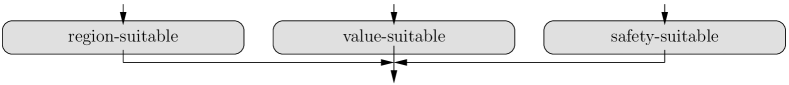
Figure 8: The interface between the two stages of the analysis of functions.

6.1 Analyzability of Functions

Here we define and explain the three function properties that are necessary for the analysis. Their associated bounding functions constitute the interface between the two stages. Informally, the properties have the following meanings:

• We can reduce the volume of the region of uncertainty to any arbitrarily small value (region-suitability).

• There are positive and finite limits on the absolute value of $f$ outside of the region of uncertainty (value-suitability).

• We can reduce the rounding error in the floating-point evaluation of $f$ to any arbitrarily small value (safety-suitability).

The region-suitability

The region-suitability is a geometric condition on the neighborhood of the critical set. We demand that we can adjust the volume of the region of uncertainty to any arbitrarily small value. For technical reasons we need an invertible bound.

Definition 13 (region-suitable)

Let ${(f,k,A,\delta,{e_{\text{\rm max}}},{\Gamma\text{\rm-line}},t)}$ be a predicate description. We call $f$ region-suitable if the critical set of $f$ is either empty or if there is an invertible upper-bounding function

$$\nu_{f}:{\Gamma\text{\rm-line}}\to\mathbb{R}_{>0}$$

on the volume of the region of uncertainty that has the property: For every $p\in(0,1)$ there is $\gamma\in{\Gamma\text{\rm-line}}$ such that

$$\frac{\mu(R_{\gamma}(\bar{x}))}{\mu(U_{\delta}(\bar{x}))} \leq \frac{\nu_{f}(\gamma)}{\mu(U_{\delta}(\bar{x}))}\;\;\leq\;\;(1-p)$$ (18)

for all $\bar{x}\in A$.

Remark 3

We add several remarks on the definition above.

1. Region-suitability is related to the region-condition in the following way: The criterion for region-suitability results from the replacement of $\mu(R_{\gamma}(\bar{x}))$ in Formula (11) with a function $\nu_{f}$. This changes the region-condition in Definition 11 into a quantitative bound.

2. Of course, controlled perturbation cannot work if the region of uncertainty covers the entire perturbation area of $\bar{x}$. We have said that we consider $\gamma\in{\Gamma\text{\rm-line\,}_{\hat{\gamma}}}$ for a “sufficiently” small $\hat{\gamma}\in\mathbb{R}_{>0}^{k}$. That means formally, we postulate $\nu(\hat{\gamma})\ll\mu(U_{\delta}(\bar{x}))$. To keep the notation as plain as possible, we are aware of this fact and do not make this condition explicit in our statements.

3. The invertibility of the bonding function $\nu_{f}$ is essential for the method of quantified relations as we see in the proof of Theorem 7.1. There it is used to deduce the parameter $\gamma$ from the volume of the region of uncertainty—with the exception of an empty critical set which does not imply any restriction on $\gamma$.

4a. The function $\nu_{f}$ provides an upper bound on the volume of the region of uncertainty within the perturbation area of $\bar{x}$. Sometimes it is more convenient to consider its complement

$$\chi_{f}(\gamma) := \mu\left(U_{\delta}(\bar{x})\right)\,-\,\nu_{f}(\gamma).$$ (19)

The function $\chi_{f}(\gamma)$ provides a lower bound on the volume of the region of provable fp-safe inputs.

4b. The special case $\nu_{f}\equiv 0$ corresponds to the special case $\chi_{f}\equiv\mu\left(U_{\delta}(\bar{x})\right)$. Then the critical set is empty and there is no region of uncertainty. This implies that $\varphi_{f}(\gamma)$ can also be chosen as a constant function (see the value-suitability below).

4c. Based on Formula (19), we can demand the existence of an invertible function $\chi_{f}:{\Gamma\text{\rm-line}}\to\mathbb{R}_{>0}$ instead of $\nu_{f}$ in the definition of region-suitability. That means, either $\chi_{f}\equiv\mu\left(U_{\delta}(\bar{x})\right)$ or $\chi_{f}:{\Gamma\text{\rm-line}}\to\mathbb{R}_{>0}$ in an invertible function.

5. We make the following observations about region-suitability: (a) If the critical set is finite, $f$ is region-suitable. (b) If the critical set contains an open set, $f$ cannot be region-suitable. (c) If the critical set is a set of measure zero, it does not imply that $f$ is region-suitable. Be aware that these properties are not equivalent: If $f$ is region-suitable, the critical set is a set of measure zero. But a critical set of measure zero does not necessarily imply that $f$ is region-suitable: In topology we learn that $\mathbb{Q}$ is dense in $\mathbb{R}$; hence any open $\varepsilon$-neighborhood of $\mathbb{Q}$ equals $\mathbb{R}$. In set theory we learn that $|\mathbb{Q}|=\aleph_{0}<2^{\aleph_{0}}=|\mathbb{R}|$; hence $f$ cannot be region-suitable if the critical set is (locally) “too dense.” $\bigcirc$

The inf-value-suitability

The inf-value-suitability is a condition on the behavior of the function $f$. We demand that there is a positive lower bound on the absolute value of $f$ outside of the region of uncertainty.

Definition 14 (inf-value-suitable)

Let ${(f,k,A,\delta,{e_{\text{\rm max}}},{\Gamma\text{\rm-line}},t)}$ be a predicate description. We call $f$ (inf-)value-suitable if there is a lower-bounding function

$$\varphi_{\inf f}:{\Gamma\text{\rm-line}}\to\mathbb{R}_{>0}$$

on the absolute value of $f$ that has the property: For every $\gamma\in{\Gamma\text{\rm-line}}$, we have

$$\varphi_{\inf f}(\gamma) \leq |f(x)|$$ (20)

for all $x\in\bar{U}_{\delta}(\bar{x})\setminus R_{\gamma}(\bar{x})$ and for all $\bar{x}\in A$.

We extend this definition by an upper bound on the absolute value of $f$ in Section 12 and call this property sup-value-suitability; until then we call the inf-value-suitability simply the value-suitability and also write $\varphi_{f}$ instead of $\varphi_{\inf f}$. The criterion for value-suitability results from the replacement of the constant $\varphi$ in Formula (14) with the bounding function $\varphi_{f}$. This changes the existence statement of Lemma 1 into a quantitative bound.

The inf-safety-suitability

The inf-safety-suitability is a condition on the error analysis of the floating-point evaluation of $f$. We demand that we can adjust the rounding error in the evaluation of $f$ to any arbitrarily small value. For technical reasons we demand an invertible bound.

Definition 15 (inf-safety-suitable)

Let ${(f,k,A,\delta,{e_{\text{\rm max}}})}$ be a predicate description. We call $f$ (inf-)safety-suitable if there is an injective fp-safety bound $S_{\inf f}(L):\mathbb{N}\to\mathbb{R}_{>0}$ that fulfills the safety-condition in Formula (12) and if

$$S_{\inf f}^{-1}:(0,S_{\inf f}(1)]\to\mathbb{R}_{>0}.$$

is a strictly monotonically decreasing real continuation of its inverse.

We extend the definition by sup-safety-suitability in Section 12; until then we call the inf-safety-suitability simply the safety-suitability.

The analyzability

Based on the definitions above, we next define analyzability, relate it to verifiability and give an example for the definitions.

Definition 16 (analyzable)

We call $f$ analyzable if it is region-, value- and safety-suitable.

Lemma 3

Let $f$ be analyzable. Then $f$ is verifiable.

Proof

If $f$ is analyzable, $f$ is especially region-suitable. Then the region-condition in Definition 11 is fulfilled because of the bounding function $\nu_{f}$. In addition $f$ must also be safety-suitable. Then the safety-condition in Definition 11 is fulfilled because of the bounding function $S_{\inf f}$. Together both conditions imply that $f$ is verifiable. ∎

We support the definitions above with the example of univariate polynomials. Because we refer to this example later on, we formulate it as a lemma.

Lemma 4

Let $f$ be the univariate polynomial

$$f(x) = a_{d}\cdot x^{d}+a_{d-1}\cdot x^{d-1}+\ldots+a_{1}\cdot x+a_{0}$$ (21)

of degree $d$ and let ${(f,k,A,\delta,{e_{\text{\rm max}}},{\Gamma\text{\rm-line}},t)}$ be a predicate description for $f$. Then $f$ is analyzable on $\bar{U}_{\delta}(A)$ with the following bounding functions

$$\nu_{f}(\gamma) := 2d\gamma$$ (22)

$$\varphi_{f}(\gamma) := |a_{d}|\cdot\gamma^{d}$$ (23)

$$S_{\inf f}(L) := (d+2)\,\max_{1\leq i\leq d}|a_{i}|\;\,2^{{e_{\text{\rm max}}}(d+1)+1-L}.$$

Proof

For a moment we consider the complex continuation of the polynomial, i.e. $f\in\mathbb{C}[z]$. Because of the fundamental theorem of algebra (e.g., see Lamprecht [41]), we can factorize $f$ in the way

$$f(z) = a_{d}\cdot\prod_{i=1}^{d}(z-\zeta_{i})$$

since $f$ has $d$ (not necessarily distinct) roots $\zeta_{i}\in\mathbb{C}$. Now let $\gamma\in\mathbb{R}_{>0}$. Then we can lower bound the absolute value of $f$ by

$$|f(z)| \geq |a_{d}|\cdot\gamma^{d}$$

for all $z\in\mathbb{C}$ whose distance to every (complex) root of $f(z)$ is at least $\gamma$. Naturally, the last estimate is especially true for real arguments $x$ whose distance to the orthogonal projection of the complex roots $\zeta_{i}$ onto the real axis is at least $\gamma$. So we set the critical set to $C_{f}(\bar{x}):=\{\text{\rm Re}(\zeta_{i}):1\leq i\leq d\}\cap\bar{U}_{\delta}(\bar{x})$. This validates the bound $\varphi_{f}$ and implies that $f$ is value-suitable.

Furthermore, the size of $C_{f}$ is upper-bounded by $d$ for all $\bar{x}\in A$. This validates the bound $\nu_{f}$. Because $\nu_{f}$ is invertible, $f$ is region-suitable.

The bounding function $S_{\inf f}(L)$ is proven in Corollary 3 in Section 11. Because $S_{\inf f}(L)$ is invertible, $f$ is also safety-suitable. As a consequence, $f$ is analyzable with the given bounds. ∎

We admit that we have chosen a quite simple example. But a more complex example would have been a waste of energy since we present three general approaches to derive the bounding functions for the region- and value-suitability in Sections 8, 9 and 10. That means, for more complex examples we use more convenient tools. A well-known approach to derive the bounding function for the safety-bound is given in Section 11.

6.2 Overview: Function Properties

At this point, we have introduced all properties that are necessary to precisely characterize functions in the context of the analysis. So let us take a short break to see what we have defined and related so far. We have summarized the most important implications in Figure 9.

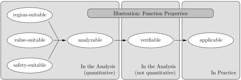
Figure 9: The illustration summarizes the implications of the various function properties that we have defined in this paper. A function that is region-, value- and safety-suitable at the same time is also analyzable (see Definition 16). An analyzable function is also verifiable (see Lemma 3). And a verifiable function is also applicable (see Lemma 2).

Controlled perturbation is applicable to a certain class of functions. But only for a subset of those functions, we can actually verify that controlled perturbation works in practice—without the necessity, or even ability, to analyze their performance. We remember that no condition on the absolute value is needed for verifiability because it is not a quantitative property. A subset of the verifiable functions represents the set of analyzable functions in a quantitative sense. For those functions there are suitable bounds on the maximum volume of the region of uncertainty, on the minimum absolute value outside of this region and on the maximum rounding error. In the remaining part of the paper, we are only interested in the class of analyzable functions.

7 The Method of Quantified Relations

The method of quantified relations actually performs the function analysis in the second stage. The component and its interface are illustrated in Figure 10. We introduce the method in Section 7.1. Its input consists of three bounding functions that are associated with the three suitability properties from the last section. The applicability does not depend on any other condition. The method provides general instructions to relate the three given bounds. The prime objective is to derive a relation between the probability of a successful floating-point evaluation and the precision of the floating-point arithmetic. More precisely, the method provides a precision function $L(p)$ or a probability function $p(L)$. This is the first presentation of step-by-step instructions for the second stage of the function analysis. An example of its application follows in Section 7.2.

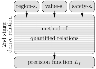
Figure 10: The method of quantified relations and its interface.

7.1 Presentation

There are no further prerequisites than the three necessary suitability properties from the last section. Therefore we can immediately state the main theorem of this section whose proof contains the method of quantified relations.

Theorem 7.1 (quantified relations)

Let ${(f,k,A,\delta,{e_{\text{\rm max}}},{\Gamma\text{\rm-line}},t)}$ be a predicate description and let $f$ be analyzable. Then there is a method to determine a precision function $L_{f}:(0,1)\to\mathbb{N}$ such that the guarded evaluation of $f$ at a randomly perturbed input is successful with probability at least $p\in(0,1)$ for every precision $L\in\mathbb{N}$ with $L\geq L_{f}(p)$.

Proof

We show in six steps how we can determine a precision function $L_{f}(p)$ which has the property: If we use a floating-point arithmetic with precision $L_{f}(p)$ for a given $p\in(0,1)$, the evaluation of $f(x)\!|_{\mathbb{G}}$ is guarded with success probability of at least $p$ for a randomly chosen $x\in\bar{U}_{\delta}(\bar{x})\!|_{\mathbb{G}}$ and for any $\bar{x}\in A$. An overview of the steps is given in Table 1. Usually we begin with Step 1. However, there is an exception: In the special case that $\nu_{f}\equiv 0$, we know that the bounding function $\varphi$ is constant, see Remark 3.4 for details. Then we just skip the first four steps and begin with Step 5.

Step 1: relate probability with volume of region of uncertainty (define ${\varepsilon_{\nu}}$) Step 2: relate volume of region of uncertainty with distances (define $\gamma$) Step 3: relate distances with floating-point grid (choose $t$) Step 4: relate new distances with minimum absolute value (define $\varphi$) Step 5: relate minimum absolute value with precision (define ${L_{\text{\rm safe}}}$) Step 6: relate ${L_{\text{\rm safe}}}$ with ${L_{\text{\rm grid}}}$ (define ${L_{\text{\rm grid}}}$ and $L_{f}$)

Table 1: Instructions for performing the method of quantified relations.

Step 1 (define ${\varepsilon_{\nu}}$). We derive an upper bounding function ${\varepsilon_{\nu}(p)}$ on the volume of the augmented region of uncertainty from the success probability $p$ in the way

$${\varepsilon_{\nu}(p)} := (1-p)\cdot\mu(U_{\delta})$$

$$= (1-p)\cdot\prod_{i=1}^{k}(2\delta_{i}).$$

That means, a randomly chosen point $x\in U_{\delta}(\bar{x})$ lies inside of a given region of volume $\varepsilon_{\nu}(p)$ with probability at least $p$. Be aware that we argue about the real space in this step.

Step 2 (define $\gamma$). We know that there is $\gamma\in\mathbb{R}_{>0}^{k}$ that fulfills the region-condition in Definition 11 because $f$ is verifiable. Since $f$ is even region-suitable, we can also determine such $\gamma\in{\Gamma\text{\rm-line}}$ by means of the inverse of the bounding function $\nu_{f}$. The existence and invertibility of $\nu_{f}$ is guaranteed by Definition 13. Hence we define the function

$$\gamma(p) := \nu_{f}^{-1}({\varepsilon_{\nu}(p)})\in{\Gamma\text{\rm-line}}.$$ (25)

We remember that there is an alternative definition of the region-suitability which we have mentioned in Remark 3.4. Surely it is also possible to use the bounding function $\chi_{f}$ instead of $\nu_{f}$ in the method of quantified relations directly; the alternative Steps $1^{\prime}$ and $2^{\prime}$ are introduced in Remark 4.2.

Step 3 (choose $t$). We aim at a result that is valid for floating-point arithmetic although we base the analysis on real arithmetic (see Section 5). We choose $t\in(0,1)$ and define $R_{t\gamma}$ as the normal sized region of uncertainty. Due to Theorem 5.1, the probability that a random point $x\in U_{\delta}(\bar{x})\!|_{\mathbb{G}}$ lies inside of $R_{t\gamma}(\bar{x})\!|_{\mathbb{G}}$ is smaller than the probability that a random point $x\in U_{\delta}(\bar{x})$ lies inside of $R_{\gamma}(\bar{x})$. Consequently, if a randomly chosen point lies outside of the augmented region of uncertainty with probability $p$, it lies outside of the normal sized region of uncertainty with probability at least $p$. Our next objective is to guarantee a floating-point safe evaluation outside of the normal sized region of uncertainty.

Step 4 (define $\varphi$). Now we want to determine the minimum absolute value outside of the region of uncertainty $R_{t\gamma}(\bar{x})$. We have proven in Lemma 1 that a positive minimum exists. Because $f$ is value-suitable, we can use the bounding function $\varphi_{f}$ for its determination (see Definition 14). That means, we consider

$$\varphi(p) := \varphi_{f}(t\cdot\gamma(p)).$$

Step 5 (define ${L_{\text{\rm safe}}}$). So far we have fixed the region of uncertainty and have determined the minimum absolute value outside of this region. Now we can use the safety-condition from Definition 11 to determine a precision ${L_{\text{\rm safe}}}$ which implies fp-safe evaluations outside of $R_{t\gamma}$. That means, we want that Formula (13) is valid for every $L\in\mathbb{N}$ with $L\geq{L_{\text{\rm safe}}}$. Again we use the property that $f$ is analyzable and use the inverse of the fp-safety bound $S_{\inf f}^{-1}$ in Definition 15 to deduce the precision from the minimum absolute value $\varphi(p)$ as

$${L_{\text{\rm safe}}}(p) = \left\lceil S_{\inf f}^{-1}\left(\varphi_{f}\left(t\cdot\nu_{f}^{-1}\left({\varepsilon_{\nu}\left(p\right)}\right)\right)\right)\right\rceil.$$ (26)

Step 6 (define ${L_{\text{\rm grid}}}$ and $L_{f}$). We numerate the component functions of $\nu_{f}^{-1}$ in the way $\nu_{f}^{-1}(\varepsilon)=(\nu_{1}^{-1}(\varepsilon),\ldots,\nu_{k}^{-1}(\varepsilon))$. Then we deduce the bound ${L_{\text{\rm grid}}}$ from Formula (16) and Formula (25) in the way

$${L_{\text{\rm grid}}}(p) := {e_{\text{\rm max}}}-1-\left\lfloor\log_{2}\left(\min\left\{t,1-t\right\}\cdot\min_{1\leq i\leq k}\nu_{i}^{-1}(\varepsilon_{\nu}(p))\right)\right\rfloor.$$ (27)

Finally we define the precision function $L_{f}(p)$ pointwise as

$$L_{f}(p) := \max\left\{{L_{\text{\rm safe}}}(p),{L_{\text{\rm grid}}}(p)\right\}.$$ (28)

Due to the used estimates, any precision $L\in\mathbb{N}$ with $L\geq L_{f}(p)$ is a solution. ∎

Remark 4

We add some remarks on the theorem above.

1. It is important to see that ${L_{\text{\rm safe}}}$ is derived from the volume of $R_{f}$ and is based on the region- and safety condition in Definition 11 whereas ${L_{\text{\rm grid}}}$ is derived from the narrowest width of $R_{f}$ and is based on the grid unit condition in Section 5.1. Of course, $L_{f}(p)$ must be large enough to fulfill both constraints.

2. As we have seen, we can also use the function $\chi_{f}$ to define the region-suitability in Definition 13. Therefore we can modify the first two steps of the method of quantified relations as follows:
Step $1^{\prime}$ (define $\varepsilon_{\chi}$). Instead of Step 1, we define a bounding function ${\varepsilon_{\chi}(p)}$ on the volume of the complement of $R_{f}$ from the given success probability $p$. That means, we replace Formula (7.1) with

$${\varepsilon_{\chi}(p)} := p\cdot\mu(U_{\delta})$$

$$= p\cdot\prod_{i=1}^{k}\left(2\delta_{i}\right).$$

Step $2^{\prime}$ (define $\gamma$). Then we can determine $\gamma(p)$ with the inverse of the bounding function $\chi_{f}$. That means, we replace Formula (25) with

$$\gamma(p) := \chi_{f}^{-1}({\varepsilon_{\chi}(p)})\in{\Gamma\text{\rm-line}}$$

which finally changes Formula (26) into

$${L_{\text{\rm safe}}}(p) = \left\lceil S_{\inf f}^{-1}\left(\varphi_{f}\left(t\cdot\chi_{f}^{-1}\left({\varepsilon_{\chi}\left(p\right)}\right)\right)\right)\right\rceil.$$

We make the observation that these changes do not affect the correctness of the method of quantified relations.

3. It is important to see that the method of quantified relations is absolutely independent of the derivation of the bounding functions which are associated with the necessary suitability properties. Especially in Step 2, $\gamma$ is determined solely by means of the function $\nu^{-1}$. We illustrate this generality with the examples in Figure 11.

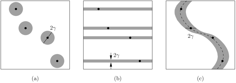
Figure 11: Visualization of $\nu^{-1}(\varepsilon_{\nu})$ in Step 2 of the method of quantified relations.

The three pictures show different regions of uncertainty for the same critical set and the same volume $\varepsilon_{\nu}$. This is because the region of uncertainties result from different functions $\nu^{-1}$. We could say that the function $\nu^{-1}$ “knows” how to distribute the region of uncertainty around the critical set because of its definition in the first stage of the analysis. For example: (a) as local neighborhoods, (b) as axis-parallel stripes, or (c) as neighborhoods of local minima of $f$ (the dashed line). (We remark that case (c) presumes that $f$ is continuous.) Naturally, different functions $\nu^{-1}$ lead to different values of $\gamma$ as is illustrated in the pictures. Be aware that the method of quantified relations itself is absolutely independent of the derivation of $\nu$ and especially independent of the approach by which $\nu$ is derived. (We present three different approaches soon.)

4. If $f$ is analyzable and $\varphi_{f}$ invertible, we can also derive the success probability $p$ from a precision $L$. We observe that the function $\varepsilon_{\nu}$ in Formula (7.1) is always invertible. Therefore we can transform Formula (26) and (27) into

$${p_{\text{\rm inf}}}(L) := \varepsilon_{\nu}^{-1}\left(\nu_{f}\left(\frac{1}{t}\cdot\varphi_{f}^{-1}\left(S_{\inf f}(L)\right)\right)\right)$$

$${p_{\text{\rm grid}}}(L) := \varepsilon_{\nu}^{-1}\left(\nu_{*}\left(\frac{2^{-L+{e_{\text{\rm max}}}-1}}{\min\{t,1-t\}}\right)\right),$$

respectively, where $\nu_{*}^{-1}$ is the least growing component function of $\nu_{f}^{-1}$ and $\nu_{*}$ is the inversion of $\nu_{*}^{-1}$. This leads to the (preliminary) probability function $p_{f}:\mathbb{N}\to(0,1)$,

$$p_{f}(L) := \min\left\{{p_{\text{\rm inf}}}(L),{p_{\text{\rm grid}}}(L)\right\}$$

for parameter $t\in(0,1)$. We develop the final version of the probability function in Section 12.2. Self-evidently we can also derive appropriate bounding functions for $\chi$ instead of $\nu$ (see Remark 2). $\bigcirc$

7.2 Example

To get familiar with the usage of the method of quantified relations, we give a detailed application in the proof of the following lemma.

Lemma 5

Let $f$ be a univariate polynomial of degree $d$ as shown in Formula (21) and let ${(f,k,A,\delta,{e_{\text{\rm max}}},{\Gamma\text{\rm-line}},t)}$ be a predicate description. Then we obtain for $f$:

$${L_{\text{\rm safe}}}(p) := \left\lceil-d\log_{2}(1-p)\;+\;{c_{\text{\rm u}}}\right\rceil$$ (29)

where

$${c_{\text{\rm u}}} := \log_{2}\frac{(d+2)\cdot\max_{1\leq i\leq d}|a_{i}|\cdot 2^{{e_{\text{\rm max}}}(d+1)+1}}{|a_{d}|\cdot(t\delta/d)^{d}}.$$

Proof

The polynomial $f$ is analyzable because of Lemma 4. Therefore we can determine ${L_{\text{\rm safe}}}$ with the first 5 steps of the method of quantified relations (see Theorem 7.1).
Step 1: Since the perturbation area $U_{\delta}(\bar{x})$ is an interval of length $2\delta$, the region of uncertainty has a volume of at most

$${\varepsilon_{\nu}(p)} := 2\delta(1-p).$$

Step 2: Next we deduce $\gamma$ from the inverse of the function in Formula (22), that means, from $\nu_{f}^{-1}(\varepsilon)=\frac{\varepsilon}{2d}$. We obtain

$$\gamma(p) := \nu^{-1}_{f}({\varepsilon_{\nu}(p)})\;\;=\;\;\frac{{\varepsilon_{\nu}(p)}}{2d}\;\;=\;\;\frac{\delta(1-p)}{d}.$$

Step 3: We choose $t\in(0,1)$.
Step 4: Due to Formula (23), the absolute value of $f$ outside of the region of uncertainty is lower-bounded by the function

$$\varphi(p) := |a_{d}|\cdot(t\cdot\gamma(p))^{d}$$

$$= |a_{d}|\cdot\left(\frac{t\delta(1-p)}{d}\right)^{d}.$$

Step 5: A fp-safety bound $S_{\inf f}$ is provided by Corollary 3 in Formula (59). The inverse of this function at $\varphi(p)$ is

$$S_{\inf f}^{-1}(\varphi(p)) = \log_{2}\frac{(d+2)\cdot\max_{1\leq i\leq d}|a_{i}|\cdot 2^{{e_{\text{\rm max}}}(d+1)+1}}{\varphi(p)}.$$

Due to Formula (26), this leads to

$${L_{\text{\rm safe}}}(p) := \left\lceil S_{\inf f}^{-1}(\varphi(p))\right\rceil$$

$$= \left\lceil\log_{2}\frac{(d+2)\cdot\max_{1\leq i\leq d}|a_{i}|\cdot 2^{{e_{\text{\rm max}}}(d+1)+1}}{|a_{d}|\cdot(t\delta(1-p)/d)^{d}}\right\rceil$$

$$= \left\lceil-d\log_{2}(1-p)\;+\;\log_{2}\frac{(d+2)\cdot\max_{1\leq i\leq d}|a_{i}|\cdot 2^{{e_{\text{\rm max}}}(d+1)+1}}{|a_{d}|\cdot(t\delta/d)^{d}}\right\rceil$$

as was claimed in the lemma. ∎

Since the formula for ${L_{\text{\rm safe}}}(p)$ in the lemma above looks rather complicated, we interpret it here. We observe that $c_{u}$ is a constant because it is defined only by constants: The degree $d$ and the coefficients $a_{i}$ are defined by $f$, and the parameters ${e_{\text{\rm max}}}$ and $\delta$ are given by the input. We make the asymptotic behavior ${L_{\text{\rm safe}}}(p)=O\left(-d\log_{2}(1-p)\right)$ for $p\to 1$ explicit in the following corollary: We show that $d$ additional bits of the precision are sufficient to halve the failure probability.

Corollary 1

Let $f$ be a univariate polynomial of degree $d$ and let ${L_{\text{\rm safe}}}:(0,1)\to\mathbb{N}$ be the precision function in Formula (29). Then

$${L_{\text{\rm safe}}}\left(\frac{1+p}{2}\right) = {L_{\text{\rm safe}}}(p)+d.$$

Proof

Due to Formula (29) we have:

$${L_{\text{\rm safe}}}\left(\frac{1+p}{2}\right) = \left\lceil-d\log_{2}\left(1-\left(\frac{1+p}{2}\right)\right)+c_{u}\right\rceil$$

$$= \left\lceil-d\log_{2}\left(\frac{1-p}{2}\right)+c_{u}\right\rceil$$

$$= \left\lceil-d\left(\log_{2}(1-p)-\log_{2}(2)\right)+c_{u}\right\rceil$$

$$= \left\lceil-d\log_{2}(1-p)+d+c_{u}\right\rceil$$

$$= \left\lceil-d\log_{2}(1-p)+c_{u}\right\rceil+d$$

$$= {L_{\text{\rm safe}}}(p)+d$$

Because $d$ is a natural number, we can pull it out of the brackets. ∎

8 The Direct Approach Using Estimates

This approach derives the bounding functions which are associated with region- and value-suitability in the first stage of the analysis (see Figure 12). It is partially based on the geometric interpretation of the function $f$ at hand. More precisely, it presumes that the critical set of $f$ is embedded in geometric objects for which we know simple mathematical descriptions (e.g., lines, circles, etc.). The derivation of bounds from geometric interpretations is also presented in [45, 46]. In Section 8.1 we explain the derivation of the bounds. In Section 8.2 we show some examples.

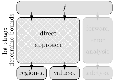
Figure 12: The direct approach and its interface.

8.1 Presentation

The steps of the direct approach are summarized in Table 2. To facilitate the presentation of the geometric interpretation, we assume that the function $f$ is continuous everywhere and that we do not allow any exceptional points. Then the critical set of $f$ equals the zero set of $f$. Hence the region of uncertainty is an environment of the zero set in this case. We define the region of uncertainty $R_{\gamma}$ as it is defined in Formula (10). In the first step, we choose ${\Gamma\text{\rm-line}}$ which is the domain of $\gamma$. Or in other words, we choose $\hat{\gamma}$. Sometimes, certain choices of ${\Gamma\text{\rm-line}}$ may be more useful than others, e.g., cubic environments where $\hat{\gamma}_{i}=\hat{\gamma}_{j}$ for all $1\leq i,j\leq k$.

Now assume that we have chosen ${\Gamma\text{\rm-line}}$. In the second step, we estimate (an upper bound on) the volume of the region of uncertainty $R_{\gamma}$ by a function $\nu_{f}(\gamma)$ for $\gamma\in{\Gamma\text{\rm-line}}$. In the direct approach, we hope that a geometric interpretation of the zero set supports the estimation. For that purpose it would be helpful if the region of uncertainty is embedded in a line, a circle, or any other geometric structure that we can easily describe mathematically.

Assume further that we have fixed the bound $\nu_{f}$. In the third step, we need to determine a function $\varphi_{f}(\gamma)$ on the minimum absolute value of $f$ outside of $R_{\gamma}$. This is the most difficult step in the direct approach: Although geometric interpretation may be helpful in the second step, mathematical considerations are necessary to derive $\varphi_{f}$. Therefore we hope that $\varphi_{f}$ is “obvious” enough to get guessed. If there is no chance to guess $\varphi_{f}$, we need to try one of the alternative approaches of the next sections, that means, the bottom-up approach or the top-down approach.

Step 1: choose the set ${\Gamma\text{\rm-line}}$ (define $\hat{\gamma}$) Step 2: estimate $\nu_{f}(\gamma)$ in dependence on ${\Gamma\text{\rm-line}}$ (define $\nu_{f}$) Step 3: estimate $\varphi_{f}(\gamma)$ in dependence on $\nu_{f}(\gamma)$ (define $\varphi_{f}$)

Table 2: Instructions for performing the direct approach.

8.2 Examples

We present two examples that use the direct approach to derive the bounds for the region-value-suitability.

Example 7

We consider the in_box predicate in the plane. Let $u$ and $v$ be two opposite vertices of the box and let $q$ be the query point. Then $\text{\rm in\_box}(u,v,q)$ is decided by the sign of the function

$$f(u,v,q) = f({u_{x}},{u_{y}},{v_{x}},{v_{y}},{q_{x}},{q_{y}})$$ (30)

$$:= \max\left\{\left({q_{x}}-{u_{x}}\right)\left({q_{x}}-{v_{x}}\right),\;\left({q_{y}}-{u_{y}}\right)\left({q_{y}}-{v_{y}}\right)\right\}.$$

The function is negative if $x$ lies inside of the box, it is zero if $x$ lies in the boundary, and it is positive if $x$ lies outside of the box.

Step 1: We choose an arbitrary $\hat{\gamma}=(\hat{\gamma}_{u_{x}},\hat{\gamma}_{u_{y}},\hat{\gamma}_{v_{x}},\hat{\gamma}_{v_{y}},\hat{\gamma}_{q_{x}},\hat{\gamma}_{q_{y}})\in\mathbb{R}_{>0}^{6}$.

Step 2: The box is defined by $u$ and $v$. This fact is true independent of the choices for $\gamma_{u_{x}}$, $\gamma_{u_{y}}$, $\gamma_{v_{x}}$ and $\gamma_{v_{y}}$. We observe that the largest box inside of the perturbation area $U_{\delta}$ is the boundary of $U_{\delta}$ itself. This observation leads to the upper bound

$$\nu_{f}(\gamma) = \nu_{f}(\gamma_{u_{x}},\gamma_{u_{y}},\gamma_{v_{x}},\gamma_{v_{y}},\gamma_{q_{x}},\gamma_{q_{y}})$$

$$:= 4\left(\gamma_{q_{x}}\delta_{y}\;+\;\gamma_{q_{y}}\delta_{x}\right)$$

on the volume of the region of uncertainty if we take the horizontal distance $\gamma_{q_{x}}$ and the vertical distance $\gamma_{q_{y}}$ from the boundary of the box into account. That means, $\nu_{f}$ depends on the distances $\gamma_{q_{x}}$ and $\gamma_{q_{y}}$ of the query point $q$ from the zero set.

Step 3: The evaluation of Formula (30) at query points where ${q_{x}}$ has distance $\gamma_{q_{x}}$ from ${u_{x}}$ or ${v_{x}}$, and ${q_{y}}$ has distance $\gamma_{q_{y}}$ from ${u_{y}}$ or ${v_{y}}$, leads to

$$\varphi_{f}(\gamma) := \min\left\{\left|\gamma^{2}_{q_{x}}-\gamma_{q_{x}}\cdot|{v_{x}}-{u_{x}}|\right|,\;\left|\gamma^{2}_{q_{y}}-\gamma_{q_{y}}\cdot|{v_{y}}-{u_{y}}|\right|\right\}.$$

The derived bounds fulfill the desired properties. $\bigcirc$

Example 8

We consider the in_circle predicate in the plane. Let $c$ be the center of the circle, let $r>0$ be its radius, and let $q$ be the query point. Then $\text{\rm in\_circle}(c,r,q)$ is decided by the sign of the function

$$f(c,r,q) = f({c_{x}},{c_{y}},r,{q_{x}},{q_{y}})$$ (31)

$$:= \left({q_{x}}-{c_{x}}\right)^{2}\;+\;\left({q_{y}}-{c_{y}}\right)^{2}\;-\;r^{2}$$

The function is negative if $x$ lies inside of the circle, it is zero if $x$ lies on the circle, and it is positive if $x$ lies outside of the circle.

Step 1: We choose $\hat{\gamma}=(\hat{\gamma}_{c_{x}},\hat{\gamma}_{c_{y}},\hat{\gamma}_{r},\hat{\gamma}_{q_{x}},\hat{\gamma}_{q_{y}})\in\mathbb{R}_{>0}^{5}$ where $\hat{\gamma}_{q_{x}}=\hat{\gamma}_{q_{y}}$. In addition, we choose $\hat{\gamma}_{r}<r$ for simplicity.

Step 2: The largest circle that fits into the perturbation area $U_{\delta}$ has radius $\min\left\{\delta_{x},\delta_{y}\right\}$. If we intersect any larger circle with $U_{\delta}$, the total length of the circular arcs inside of $U_{\delta}$ cannot be larger than $2\pi\cdot\min\left\{\delta_{x},\delta_{y}\right\}$. This bounds the total length of the zero set.

Now we define the region of uncertainty by spherical environments: The region of uncertainty is the union of open discs of radius $\gamma_{q_{x}}$ which are located at the zeros. Then the width of the region of uncertainty is given by the diameter of the discs, i.e., by $2\gamma_{q_{x}}$. As a consequence,

$$\nu_{f}(\gamma) = \nu_{f}(\gamma_{c_{x}},\gamma_{c_{y}},\gamma_{r},\gamma_{q_{x}},\gamma_{q_{y}})$$

$$:= 4\pi\gamma_{q_{x}}\cdot\min\left\{\delta_{x},\delta_{y}\right\}$$

is an upper bound on the volume of $R_{\delta}$. That means, $\nu_{f}$ depends on the distance $\gamma_{q_{x}}$ of the query point $q$ from the zero set.

Step 3: The absolute value of Formula (31) is minimal if the query point $q$ lies inside of the circle and has distance $\gamma_{q_{x}}$ from it. This leads to

$$\varphi_{f}(\gamma) := \left|\left(r\;-\;\gamma_{q_{x}}\right)^{2}\;-\;r^{2}\right|$$

$$= \gamma_{q_{x}}\left(\gamma_{q_{x}}-2r\right).$$

The derived bounds fulfill the desired properties. $\bigcirc$

9 The Bottom-up Approach Using Calculation Rules

In the first stage of the analysis, this approach derives the bounding functions which are associated with the region- and value-suitability (see Figure 13). We can apply this approach to certain composed functions. That means, if $f$ is composed by $g$ and $h$, we can derive the bounds for $f$ from the bounds for $g$ and $h$ under certain conditions. We present some mathematical constructs which preserve the region- and value-suitability and introduce useful calculation rules for their bounds. Namely we introduce the lower-bounding rule in Section 9.1, the product rule in Section 9.2 and the min rule and max rule in Section 9.3. We point to a general way to formulate rules in Section 9.4. The list of rules is by far not complete. Nevertheless, they are already sufficient to derive the bounding functions for multivariate polynomials as we show in Section 9.5. With the bottom-up approach we present an entirely new approach to derive the bounding functions for the region-suitability and value-suitability. Furthermore we present a new way to analyze multivariate polynomials.

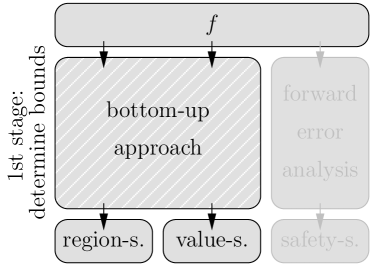
Figure 13: The bottom-up approach and its interface.

9.1 Lower-bounding Rule

Our first rule states that every function is region-value-suitable if there is a lower bounding function which is region-value-suitable. Note that there are no further restrictions on $f$.

Theorem 9.1 (lower bound)

Let ${(f,k,A,\delta,{e_{\text{\rm max}}},{\Gamma\text{\rm-line}},t)}$ be a predicate description. If there is a region-value-suitable function $g:\bar{U}_{\delta}(A)\to\mathbb{R}$ and $c\in\mathbb{R}_{>0}$ where

$$|f(x)| \geq c\,|g(x)|,$$ (32)

then $f$ is also region-value-suitable with the following bounding functions:

$$\nu_{f}(\gamma) := \nu_{g}(\gamma)$$

$$\varphi_{f}(\gamma) := c\varphi_{g}(\gamma).$$

If $f$ is in addition safety-suitable, $f$ is analyzable.

Proof

Part 1 (region-suitable). Let $(a_{i})_{i\in\mathbb{N}}$ be a sequence in the set $U_{\delta}(\bar{x})$ with $\lim_{i\to\infty}f(a_{i})=0$. Then Formula (32) implies that $\lim_{i\to\infty}g(a_{i})=0$. That means, critical points of $f$ are critical points of $g$. Therefore we set $C_{f}(\bar{x}):=C_{g}(\bar{x})$. As a consequence the region bound $\nu_{f}(\gamma):=\nu_{g}(\gamma)$ is sufficient for the region-suitability of $f$.

Part 2 (value-suitable). Because we set $C_{f}(\bar{x})=C_{g}(\bar{x})$, we have $R_{f}(\bar{x})=R_{g}(\bar{x})$. Due to Formula (32), the minimum absolute value of $f$ outside of the region of uncertainty $R_{f}(\bar{x})$ is bounded by the minimum absolute value of $g$ outside of the (same) region of uncertainty $R_{g}(\bar{x})$. Hence the bound $\varphi_{f}(\gamma)=c\varphi_{g}(\gamma)$ is sufficient for the value-suitability of $f$.

Part 3 (analyzable). Trivial. ∎

9.2 Product Rule

The next rule states that the product of region-value-suitable functions is also region-value-suitable. Furthermore, we show how to derive appropriate bounds.

Theorem 9.2 (product)

Let $(f,k,A_{g}\times A_{gh}\times A_{h},\delta,{e_{\text{\rm max}}},{\Gamma\text{\rm-line}},t)$ be a predicate description where $A_{g}\subset\mathbb{R}^{j}$, $A_{gh}\subset\mathbb{R}^{\ell-j}$ and $A_{h}\subset\mathbb{R}^{k-\ell}$ for $j\in\mathbb{N}_{0}$ and $\ell,k\in\mathbb{N}$ with $j\leq\ell\leq k$. If there are two region-value-suitable functions

$$g : \bar{U}_{(\delta_{1},\ldots,\delta_{\ell})}(A_{g}\times A_{gh})\to\mathbb{R}$$

$$h : \bar{U}_{(\delta_{j+1},\ldots,\delta_{k})}(A_{gh}\times A_{h})\to\mathbb{R}$$

such that

$$f(x_{1},\ldots,x_{k}) = g(x_{1},\ldots,x_{\ell})\cdot h(x_{j+1},\ldots,x_{k}),$$

then $f$ is also region-value-suitable with the following bounding functions:

$$\varphi_{f}(\gamma) := \varphi_{g}(\gamma_{1},\ldots,\gamma_{\ell})\cdot\varphi_{h}(\gamma_{j+1},\ldots,\gamma_{k})$$ (33)

$$\nu_{f}(\gamma) := \min\left\{\prod_{i=1}^{k}(2\delta_{i}),\right.$$ (34)

$$\qquad\left.\nu_{g}(\gamma_{1},\ldots,\gamma_{\ell})\!\!\!\prod_{i=\ell+1}^{k}\!\!\!(2\delta_{i})\,+\,\nu_{h}(\gamma_{j+1},\ldots,\gamma_{k})\prod_{i=1}^{j}(2\delta_{i})\right\}.$$

Furthermore, if $j=\ell$, we can replace the last equation by the tighter bound

$$\chi_{f}(\gamma) := \chi_{g}(\gamma_{1},\ldots,\gamma_{j})\cdot\chi_{h}(\gamma_{j+1},\ldots,\gamma_{k}).$$ (35)

If $f$ is in addition safety-suitable, $f$ is analyzable (independent of $j=\ell$).

Proof

Part 1 (value-suitable). Let $x\in U_{\delta}(\bar{x})$ such that $(x_{1},\ldots,x_{\ell})$ does not lie in the region of uncertainty of $g$, that means

$$(x_{1},\ldots,x_{\ell})\not\in R_{g,(\gamma_{1},\ldots,\gamma_{\ell})}(\bar{x}_{1},\ldots,\bar{x}_{\ell}),$$ (36)

and that $(x_{j+1},\ldots,x_{k})$ does not lie in the region of uncertainty of $h$, that means

$$(x_{j+1},\ldots,x_{k})\not\in R_{h,(\gamma_{j+1},\ldots,\gamma_{k})}(\bar{x}_{j+1},\ldots,\bar{x}_{k}).$$ (37)

Because $g$ and $h$ are value-suitable, we obtain:

$$|f(x)| = |g(x_{1},\ldots,x_{\ell})|\cdot|h(x_{j+1},\ldots,x_{k})|$$

$$\geq \varphi_{g}(\gamma_{1},\ldots,\gamma_{\ell})\cdot\varphi_{h}(\gamma_{j+1},\ldots,\gamma_{k})$$

$$= \varphi_{f}(\gamma)$$

on the absolute value of $f$.

Part 2 (region-suitable). Because of the argumentation above, we must construct the region of uncertainty $R_{f}$ such that $x\in\mathbb{R}^{k}$ lies outside of $R_{f}$ only if the conditions in Formula (36) and (37) are fulfilled.

Case $j=\ell$. Then the arguments of $g$ and $h$ are disjoint. This case is illustrated in Figure 14.

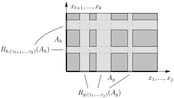
Figure 14: Case $j=\ell$: The (dark shaded) complement of $R_{f}$ is the Cartesian product of the complement of $R_{g}$ and the complement of $R_{h}$.

We observe that for each point $(x_{1},\ldots,x_{j})$ outside of $R_{g}$ and each point $(x_{\ell+1},\ldots,x_{k})$ outside of $R_{h}$ their concatenation $x$ lies outside of $R_{f}$. Therefore we determine the volume of the complement of $R_{f}$ inside of the perturbation area as

$$\mu\left(U_{f,\delta}(\bar{x})\setminus R_{f,\gamma}(\bar{x})\right) = \mu\left(U_{g,(\delta_{1},\ldots,\delta_{j})}(\bar{x}_{1},\ldots,\bar{x}_{j})\right.$$

$$\qquad\qquad\left.\setminus R_{g,(\gamma_{1},\ldots,\gamma_{j})}(\bar{x}_{1},\ldots,x_{j})\right)$$

$$\cdot\;\mu\left(U_{h,(\delta_{\ell+1},\ldots,\delta_{k})}(\bar{x}_{\ell+1},\ldots,\bar{x}_{k})\right.$$

$$\qquad\qquad\left.\setminus R_{h,(\gamma_{\ell+1},\ldots,\gamma_{k})}(\bar{x}_{\ell+1},\ldots,x_{k})\right).$$

As a consequence Formula (35) is true.

Case $j<\ell$. In contrast to the discussion above, $g$ and $h$ share the arguments $x_{j+1},\ldots,x_{\ell}$. This case is illustrated in Figure 15.

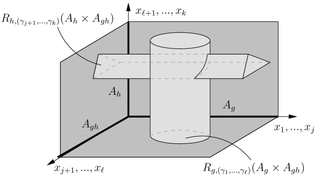
Figure 15: Case $j<\ell$: The (light shaded) region of uncertainty $R_{f}$ is the union of two Cartesian products.

We denote the projection of the first $j$ (respectively, the last $k-\ell$) coordinates by $\pi_{\leq j}$ (respectively, $\pi_{>\ell}$). In this case, Formula (35) does not have to be true. That is why we define $R_{f}$ as

$$R_{f,\gamma}(\bar{x}) := R_{g,(\gamma_{1},\ldots,\gamma_{\ell})}(\bar{x}_{1},\ldots,\bar{x}_{\ell})\times\pi_{>\ell}(\bar{U}_{\delta}(\bar{x}))$$

$$\cup\;\pi_{\leq j}(\bar{U}_{\delta}(\bar{x}))\times R_{h,(\gamma_{j+1},\ldots,\gamma_{k})}(\bar{x}_{j+1},\ldots,\bar{x}_{k}).$$

Now we can upper-bound the volume of $R_{f}$ by means of $\nu_{g}$ and $\nu_{h}$ which leads immediately to the sum in the last line of Formula (34). Of course, the volume of the region of uncertainty is bounded by the volume of the perturbation area which justifies the first line of Formula (34). This finishes the proof. ∎

9.3 Min Rule, Max Rule

The next two rules state that the minimum and maximum of finitely many region-value-suitable functions are also region-value-suitable. Furthermore, we show how to derive appropriate bounds.

Theorem 9.3 (min, max)

Let $g$ and $h$ be two region-value-suitable functions as defined in Theorem 9.2. Then the functions

$$f_{\text{\rm min}},f_{\text{\rm max}} : \bar{U}_{\delta}(A_{g}\times A_{gh}\times A_{h})\to\mathbb{R},$$

$$f_{\text{\rm min}}(x_{1},\ldots,x_{k}) := \min\{g(x_{1},\ldots,x_{\ell}),h(x_{j+1},\ldots,x_{k})\}$$

$$f_{\text{\rm max}}(x_{1},\ldots,x_{k}) := \max\{g(x_{1},\ldots,x_{\ell}),h(x_{j+1},\ldots,x_{k})\}$$

are region-value-suitable with bounds $\varphi_{f_{\text{\rm min}}}$ and $\nu_{f_{\text{\rm min}}}$ for $f_{\text{\rm min}}$ and bounds $\varphi_{f_{\text{\rm max}}}$ and $\nu_{f_{\text{\rm max}}}$ for $f_{\text{\rm max}}$ where

$$\varphi_{f_{\text{\rm min}}}(\gamma) := \min\{\varphi_{g}(\gamma_{1},\ldots,\gamma_{\ell}),\varphi_{h}(\gamma_{j+1},\ldots,\gamma_{k})\}$$

$$\varphi_{f_{\text{\rm max}}}(\gamma) := \max\{\varphi_{g}(\gamma_{1},\ldots,\gamma_{\ell}),\varphi_{h}(\gamma_{j+1},\ldots,\gamma_{k})\}$$ (38)

$$\nu_{f_{\text{\rm min}}}(\gamma):=\nu_{f_{\text{\rm max}}}(\gamma) := \nu_{f}(\gamma)\text{ (see Formula\leavevmode\nobreak\ (\ref{for-nug-plus-nuh}))}.$$

Furthermore, if $j=\ell$, we can replace $\nu_{f_{\text{\rm min}}}(\gamma)$ and $\nu_{f_{\text{\rm max}}}(\gamma)$ by the tighter bounds

$$\chi_{f_{\text{\rm min}}}(\gamma):=\chi_{f_{\text{\rm max}}}(\gamma) := \chi_{g}(\gamma_{1},\ldots,\gamma_{j})\cdot\chi_{h}(\gamma_{j+1},\ldots,\gamma_{k}).$$

If $f_{\text{\rm min}}$ (respectively $f_{\text{\rm max}}$) is in addition safety-suitable, it is also analyzable (independent of $j=\ell$).

Proof

The line of argumentation follows exactly the proof of Theorem 9.2. ∎

9.4 General Rule

We do not claim that the list of rules is complete. On the contrary, we suggest that the approach may be extended by further rules. We emphasize that the bottom-up approach is constructive: We build new region-value-suitable functions from already proven region-value-suitable functions. The argumentation always follows the proof of the product rule, that means, the compound of $g$ and $h$ inherits the desired property from $g$ and $h$: (a) outside of the union of the regions of uncertainty for shared arguments, and (b) inside of the Cartesian product of the complement of the regions of uncertainty for disjoint arguments (see Figure 14).

We remark that, if we want to derive the bounds for a specific function $f$, we first need to determine the parse tree of $f$ according to the known rules; this may be a non-obvious task in general. The instructions of the bottom-up approach are summed up in the following table.

Step 1: determine parse tree according to the rules Step 2: determine bounds bottom-up according to the parse tree

Table 3: Instructions for performing the bottom-up approach.

9.5 Example: Multivariate Polynomials

It is important to see that the rules lead to a generic approach to construct entire classes of region-value-suitable functions. In the following we use this approach to analyze multivariate polynomials. (A different way to analyze multivariate polynomials was presented before in [46].) So far we know that univariate polynomials are region-value-suitable. Now we show how we transfer the region-value-suitability property of $(k-1)$-variate polynomials to $k$-variate polynomials by means of the product rule and the lower bound rule. Moreover, we completely analyze $k$-variate polynomials afterwards.

Preparation

We prepare the analysis of multivariate polynomials with further definitions. Let $k\in\mathbb{N}$. For $\beta\in\mathbb{N}_{0}^{k}$ and $x\in\mathbb{R}^{k}$ we define $x^{\beta}$ as the term $x^{\beta}:=x_{1}^{\beta_{1}}\cdot\ldots\cdot x_{k}^{\beta_{k}}$.

Next we define the reverse lexicographic order on $k$-tuples. Let $\alpha,\beta\in\mathbb{N}_{0}^{k}$. Then we define $\alpha\,{\prec}\,\beta$ if and only if there is $\ell\in\{1,\ldots,k\}$ such that $\alpha_{j}=\beta_{j}$ for all $\ell<j\leq k$ and $\alpha_{\ell}<\beta_{\ell}$.

In addition we denote by ${\cal P}(k)$ the set of bijective functions $\sigma:\{1,\ldots,k\}\to\{1,\ldots,k\}$. In other words, ${\cal P}(k)$ is the set of permutations of $\{1,\ldots,k\}$.

Now let $\alpha,\beta\in\mathbb{N}_{0}^{k}$ and let $\sigma\in{\cal P}(k)$. We define the permutation $\sigma$ of a tuple $\alpha=(\alpha_{1},\ldots,\alpha_{k})$ by $\sigma(\alpha):=\left(\alpha_{\sigma^{-1}(1)},\ldots,\alpha_{\sigma^{-1}(k)}\right)$. Further we define the reverse lexicographic order after the permutation $\sigma$ as

$$\alpha\,{\prec}_{\sigma}\,\beta\quad :\Longleftrightarrow \quad\sigma(\alpha)\,{\prec}\,\sigma(\beta).$$

Let ${\cal I}\subset\mathbb{N}_{0}^{k}$ be finite. We denote the set of largest elements in ${\cal I}$ by

$${{\cal I}_{\rm max}} := \left\{\beta\in{\cal I}\,:\,\text{there is }\sigma\in{\cal P}(k)\text{ such that }\alpha{\prec}_{\sigma}\beta\text{ for all }\alpha\in{\cal I},\alpha\neq\beta\right\}.$$

We observe that there may be $\beta\in{\cal I}$ which do not belong to ${{\cal I}_{\rm max}}$. We observe further that different permutations may lead to the same local maximum. For each $\beta\in{{\cal I}_{\rm max}}$ we collect these permutations in the set

$${\cal P}_{\beta}(k) := \left\{\sigma\in{\cal P}(k)\,:\,\beta=\max\nolimits_{{\prec}_{\sigma}}{\cal I}\right\}.$$

The region- and value-suitability

We prove that all multivariate polynomials are region-value-suitable.

Lemma 6

Let ${(f,k,A,\delta,{e_{\text{\rm max}}},{\Gamma\text{\rm-line}},t)}$ be a predicate description for the $k$-variate polynomial ($k\geq 2$)

$$f(x):=\sum_{\iota\in{\cal I}}a_{\iota}x^{\iota}$$

where ${\cal I}\subset\mathbb{N}_{0}^{k}$ is finite and $a_{\iota}\in\mathbb{R}_{\neq 0}$ for all $\iota\in{\cal I}$. Then $f$ is region-value-suitable. There are bounding functions for every $\beta\in{{\cal I}_{\rm max}}$:

$$\varphi_{f}(\gamma) := |a_{\beta}|\cdot\gamma^{\beta}$$

$$\chi_{f}(\gamma) := \prod_{i=1}^{k}2\left(\delta_{i}-\beta_{i}\gamma_{i}\right).$$

Proof

Preparing consideration. Let $\beta\in{{\cal I}_{\rm max}}$ and let $\sigma\in{\cal P}_{\beta}(k)$. Once chosen, $\beta$ and $\sigma$ are fixed in this proof. Because of the reverse lexicographic order, the maximal exponent of $x_{\sigma(k)}$ in $f(x)$ is $\beta_{\sigma(k)}$. Therefore we can write $f$ as

$$f(x)=b_{\beta_{\sigma(k)}}\cdot x_{\sigma(k)}^{\beta_{\sigma(k)}}+b_{\beta_{\sigma(k)}-1}\cdot x_{\sigma(k)}^{\beta_{\sigma(k)}-1}+\ldots+b_{1}\cdot x_{\sigma(k)}+b_{0}$$

where the $b_{i}(x_{\sigma(1)},\ldots,x_{\sigma(k-1}))$ are $(k-1)$-variate polynomials for $0\leq i\leq\beta_{\sigma(k)}$. For a moment we consider the complex continuation of the polynomial $f$, i.e. $f\in\mathbb{C}[z]$. Furthermore we assume that the value of $b_{\beta_{\sigma(k)}}$ is not zero. Then there are $\beta_{\sigma(k)}$ (not necessarily distinct) functions $\zeta_{i}:\mathbb{C}^{k-1}\to\mathbb{C}$ such that we can write $f$ in the way

$$f(z) = b_{\beta_{\sigma(k)}}(z_{\sigma(1)},\ldots,z_{\sigma(k-1)})\cdot\prod_{i=1}^{\beta_{\sigma(k)}}(z_{\sigma(k)}-\zeta_{i}(z_{\sigma(1)},\ldots,z_{\sigma(k-1)})).$$

We remark that if we consider $f$ as a polynomial in $z_{\sigma(k)}$ with parameterized coefficients $b_{i}$, then the functions $\zeta_{i}$ define the parameterized roots. Even if the location of the roots is variable, the total number of the roots is definitely bounded by $\beta_{\sigma(k)}$. In case that $z_{\sigma(k)}$ has a distance of at least $\gamma_{\sigma(k)}$ to the values $\zeta_{i}$, we can lower bound the absolute value of $f$ by

$$|f(z)| \geq {\left|b_{\beta_{\sigma(k)}}\left(z_{\sigma(1)},\ldots,z_{\sigma(k-1)}\right)\right|}\cdot{\gamma_{\sigma(k)}^{\beta_{\sigma(k)}}}$$ (39)

Therefore this bound is especially true for real arguments. Before we end the consideration in the complex space, we add a remark. Sagraloff et al. [50, 46] suggested a way to improve this estimate: While preserving the total region-bound $\varphi_{f}$, it is possible to redistribute the region of uncertainty around the zeros of $f$ in a way where the amount of the individual region-contribution per zero may differ; they have shown that a certain redistribution improves the estimate in Formula (39). Next we use mathematical induction to prove that $f$ is region-value-suitable.

Part 1 (basis). Let $j=1$. Due to Lemma 4 univariate polynomials are region-value-suitable.

Part 2 (inductive step). Let $1<j\leq k$. We define the function $g_{j}$ as

$$g_{j}\left(z_{\sigma(1)},\ldots,z_{\sigma(j-1)}\right) := {b_{\beta_{\sigma(j)}}\left(z_{\sigma(1)},\ldots,z_{\sigma(j-1)}\right)}.$$

Since $g_{j}$ is a polynomial in $j-1$ variables, $g_{j}$ is region-value-suitable by induction. Because of Theorem 9.1, the function $|g_{j}|$ is region-value-suitable with the same bounds. Furthermore, we define the functions

$$h_{j}(z_{\sigma(j)}) := {\gamma_{\sigma(j)}^{\beta_{\sigma(j)}}}$$

$$\varphi_{h_{j}}(\gamma_{\sigma(j)}) := \gamma_{\sigma(j)}^{\beta_{\sigma(j)}}$$

$$\nu_{h_{j}}(\gamma_{\sigma(j)}) := 2\beta_{\sigma(j)}\gamma_{\sigma(j)}.$$

Obviously $h_{j}$ is region-value-suitable. We have $|f_{j}|\geq|g_{j}|\cdot h_{j}$. Then the product $|g_{j}|\cdot h_{j}$ is also region-value-suitable because of Theorem 9.2. Be aware that the construction of the estimate in Formula (39) is based on the assumption that the coefficient $b_{\beta_{\sigma(j)}}$ of $f_{j}$ is not zero. We observe that this is only guaranteed outside of the region of uncertainty of $g_{j}$. We observe further that the construction in the proof of Theorem 9.1 preserves the region of uncertainty, that means, $R_{g_{j}}\subset R_{f_{j}}$. Therefore the assumption is justified and we can conclude that $f_{j}$ is region-value-suitable. It remains to show that the claimed bounding functions $\varphi_{f}$ and $\nu_{f}$ are true.

Part 3 ($\varphi_{f}$). The basis $j=1$ follows from Lemma 4:

$$\varphi_{f_{1}}\left(\gamma_{\sigma(1)}\right) := \left|a_{\beta}\right|\cdot\gamma_{\sigma(1)}^{\beta_{\sigma(1)}}$$

(Be aware that the real coefficient $a_{\beta}$ is contained in every $g_{j}$ for $1<j\leq k$.) Now let $1<j\leq k$. For the induction step we need the following observation: Because of the reverse lexicographic order, the maximal exponent of $x_{\sigma(j-1)}$ in the parameterized coefficient $b_{\beta_{\sigma(j)}}(x_{\sigma(1)},\ldots,x_{\sigma(j-1)})$ is $\beta_{\sigma(j-1)}$. We have

$$\varphi_{f_{j}}\left(\gamma_{\sigma(1)},\ldots,\gamma_{\sigma(j)}\right) := \left|a_{\beta}\right|\cdot\prod_{\ell=1}^{j}\gamma_{\sigma(\ell)}^{\beta_{\sigma(\ell)}}$$

The case $j=k$ proves the claim.

Part 4 ($\chi_{f}$). The basis $j=1$ follows from Lemma 4:

$$\chi_{f_{1}}\left(\gamma_{\sigma(1)}\right) := 2\left(\delta_{\sigma(1)}-\beta_{\sigma(1)}\gamma_{\sigma(1)}\right).$$

Now let $1<j\leq k$. Because the argument list of $g_{j}$ and $h_{j}$ are disjoint, we apply Formula (35) and obtain

$$\chi_{f_{j}}\left(\gamma_{\sigma(1)},\ldots,\gamma_{\sigma(j)}\right) := \prod_{\ell=1}^{j}2\left(\delta_{\sigma(\ell)}-\beta_{\sigma(\ell)}\gamma_{\sigma(\ell)}\right).$$

The case $j=k$ proves the claim. ∎

The analysis

Now we prove the analyzability of multivariate polynomials and apply the approach of quantified relations to derive a precision function.

Theorem 9.4 (multivariate polynomial)

Let $f$ be a $k$-variate polynomial ($k\geq 2$) of total degree $d$ as defined in Lemma 6 and let ${(f,k,A,\delta,{e_{\text{\rm max}}},{\Gamma\text{\rm-line}},t)}$ be a predicate description for $f$ with cubical neighborhoods $\delta_{i}=\delta_{j}$ and $\gamma_{i}=\gamma_{j}$ for all $1\leq i,j\leq k$. Then $f$ is analyzable. Furthermore, we obtain the bounding function

$${L_{\text{\rm safe}}}(p) \geq \left\lceil-\beta^{*}\log_{2}\left(1-\sqrt[k]{p}\right)\;+\;{c_{\text{\rm m}}}(\beta)\right\rceil$$ (40)

where

$${c_{\text{\rm m}}}(\beta) := \log_{2}\frac{(d+1+\lceil\log_{2}|{\cal I}|\rceil)\cdot|{\cal I}|\cdot\max_{\iota\in{\cal I}}|a_{\iota}|\cdot 2^{{e_{\text{\rm max}}}d+{\beta^{*}}+1}\cdot\hat{\beta}^{\beta^{*}}}{|a_{\beta}|\cdot{(t\delta_{1})}^{\beta^{*}}}.$$

for $\beta\in{{\cal I}_{\rm max}}$ and $\hat{\beta}:=\max_{1\leq i\leq k}\beta_{i}$ and $\beta^{*}:=\sum_{1=i}^{k}\beta_{i}$.

We observe that $\hat{\beta}\leq d$ and $\beta^{*}\leq d$. Note that the choice of $\beta\in{{\cal I}_{\rm max}}$ is an optimization problem: We suggest to choose $\beta$ such that the constant $\beta^{*}$ in the asymptotic bound ${L_{\text{\rm safe}}}(p)=O\left(-\beta^{*}\log(1-\sqrt[k]{p})\right)$ for $p\to 1$ is small.

Proof

Part 1 (analyzable). Let $\beta\in{{\cal I}_{\rm max}}$. Due to Lemma 6, $f$ is region-value-suitable. In addition Corollary 4 provides a fp-safety bound $S_{\inf f}(L)$ for $k$-variate polynomials in Formula (60). The function $S_{\inf f}(L)$ converges to zero and is invertible. It follows that $f$ is safety-suitable and thus analyzable.

Part 2 (analysis). We apply the approach of quantified relations. Let $\delta_{1},\gamma_{1}\in\mathbb{R}_{>0}$ and $\delta_{1}=\delta_{i}$ and $\gamma_{1}=\gamma_{i}$ for all $1\leq i\leq k$. In addition let $\hat{\beta}:=\max_{1\leq i\leq k}\beta_{i}$. Step $1^{\prime}$: At first we derive an upper bound $\varepsilon_{\chi}$ on the volume of the complement of the region of uncertainty according to the precision $p$. Naturally we obtain

$${\varepsilon_{\chi}}(p) := p\prod_{i=1}^{k}2\delta_{i}\;\;=\;\;p\left(2\delta_{1}\right)^{k}.$$

Step $2^{\prime}$: Because of the cubical neighborhood we redefine

$$\chi_{f}(\gamma) := 2^{k}\left(\delta_{1}-\hat{\beta}\gamma_{1}\right)^{k}.$$

Then we use $\varepsilon_{\chi}$ and $\chi_{f}$ to determine $\gamma_{1}$:

$$\chi_{f}(\gamma) = {\varepsilon_{\chi}(p)}$$

$$\Leftrightarrow\makebox[85.35826pt]{\hfill$2^{k}\left(\delta_{1}-\hat{\beta}\gamma_{1}\right)^{k}$} = p\,2^{k}\,\delta_{1}^{k}$$

$$\Leftrightarrow\makebox[85.35826pt]{\hfill$\left(1-\frac{\hat{\beta}\gamma_{1}}{\delta_{1}}\right)^{k}$} = p$$

$$\Rightarrow\makebox[85.35826pt]{\hfill$1-\frac{\hat{\beta}\gamma_{1}}{\delta_{1}}$} = \sqrt[k]{p}$$

$$\Leftrightarrow\makebox[85.35826pt]{\hfill$\gamma_{1}(p)$} := \frac{\delta_{1}\left(1-\sqrt[k]{p}\right)}{\hat{\beta}}$$

Step 3: Since $\gamma$ represents the augmented region of uncertainty, the normal sized region is induced by $t\gamma$.
Step 4: Now we fix the bound $\varphi_{f}$ on the absolute value and set

$$\varphi(p) = \varphi_{f}(t\gamma(p))$$

$$= |a_{\beta}|\cdot\left(t\gamma(p)\right)^{\beta}$$

$$= |a_{\beta}|\cdot\prod_{i=1}^{k}\left(t\gamma_{i}(p)\right)^{\beta_{i}}$$

$$= |a_{\beta}|\cdot\left(t\gamma_{1}(p)\right)^{\beta^{*}}$$

$$= |a_{\beta}|\cdot\left(\frac{t\delta_{1}\left(1-\sqrt[k]{p}\right)}{\hat{\beta}}\right)^{\beta^{*}}$$

where $\beta^{*}:=\sum_{i=1}^{k}\beta_{i}$.
Step 5: To derive the bound on the precision, we consider the inverse of Formula (60) which is

$$S_{\inf f}^{-1}(\varphi(p)) = \log_{2}\frac{(d+1+\lceil\log_{2}|{\cal I}|\rceil)\cdot|{\cal I}|\cdot\max|a_{\iota}|\cdot 2^{{e_{\text{\rm max}}}d+1}}{\varphi(p)}$$

$$= \log_{2}\frac{(d+1+\lceil\log_{2}|{\cal I}|\rceil)\cdot|{\cal I}|\cdot\max|a_{\iota}|\cdot 2^{{e_{\text{\rm max}}}d+1}\cdot(2\hat{\beta})^{\beta^{*}}}{|a_{\beta}|\cdot({t\delta_{1}\left(1-\sqrt[k]{p}\right)})^{\beta^{*}}}$$

$$= -{\beta^{*}}\log_{2}{\left(1-\sqrt[k]{p}\right)}$$

$$+\log_{2}\frac{(d+1+\lceil\log_{2}|{\cal I}|\rceil)\cdot|{\cal I}|\cdot\max|a_{\iota}|\cdot 2^{{e_{\text{\rm max}}}d+1}\cdot(2\hat{\beta})^{\beta^{*}}}{|a_{\beta}|\cdot{(t\delta_{1})}^{\beta^{*}}}.$$

Finally the claim follows from ${L_{\text{\rm safe}}}(p):=\left\lceil S_{\inf f}^{-1}(\varphi(p))\right\rceil$. ∎

The formula for ${L_{\text{\rm safe}}}(p)$ in the lemma above looks rather complicated. Therefore we study the asymptotic behavior ${L_{\text{\rm safe}}}(p)=O\left(-d\log(1-\sqrt[k]{p})\right)$ for $p\to 1$ in the following corollary: We show that “slightly” more than $d$ additional bits of the precision are sufficient to halve the failure probability.

Corollary 2

Let $f$ be a $k$-variate polynomial ($k\geq 2$) of total degree $d$ and let ${L_{\text{\rm safe}}}:(0,1)\to\mathbb{N}$ be the precision function in Formula (40). Then

$${L_{\text{\rm safe}}}\left(\frac{1+p}{2}\right) \leq {L_{\text{\rm safe}}}(p)+\left\lceil\lambda\beta^{*}\right\rceil$$

where $\beta^{*}=\sum_{i=1}^{k}\beta_{i}\leq d$ and

$$\lambda := \log_{2}\left(\frac{1-\sqrt[k]{p}}{1-\sqrt[k]{\frac{1+p}{2}}}\right).$$

Proof

All quantities are as defined in Theorem 9.4. We obtain:

$${L_{\text{\rm safe}}}\left(\frac{1+p}{2}\right) = \left\lceil-\beta^{*}\log_{2}\left(1-\sqrt[k]{\frac{1+p}{2}}\right)\;+\;{c_{\text{\rm m}}}(\beta)\right\rceil$$

$$= \left\lceil-\beta^{*}\log_{2}\left(\left(1-\sqrt[k]{p}\right)\cdot\frac{1-\sqrt[k]{\frac{1+p}{2}}}{1-\sqrt[k]{p}}\right)\;+\;{c_{\text{\rm m}}}(\beta)\right\rceil$$

$$= \left\lceil-\beta^{*}\log_{2}\left(1-\sqrt[k]{p}\right)-\beta^{*}\log_{2}\left(\frac{1-\sqrt[k]{\frac{1+p}{2}}}{1-\sqrt[k]{p}}\right)\;+\;{c_{\text{\rm m}}}(\beta)\right\rceil$$

$$\leq {L_{\text{\rm safe}}}(p)+\left\lceil\beta^{*}\log_{2}\left(\frac{1-\sqrt[k]{p}}{1-\sqrt[k]{\frac{1+p}{2}}}\right)\right\rceil.$$

This proves the claim. ∎

10 The Top-down Approach Using Replacements

This approach derives the bounding functions which are associated with region- and value-suitability in the first stage of the analysis (see Figure 16). In the bottom-up approach we consider a sequence of functions which is incrementally built-up from simple functions and ends up at the function $f$ under consideration. In contrast to that we now construct a sequence of functions top-down that begins with $f$ and leads to a (different) sequence by dealing with the arguments of $f$ coordinatewise. However, the top-down approach works in two phases: In the first phase we just derive the auxiliary functions and in the second phase we determine the bounds for the region- and value-suitability bottom-up. That is why we call this approach also pseudo-top-down.

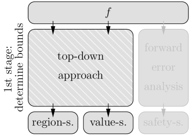
Figure 16: The top-down approach and its interface.

We remark that the idea of developing a top-down approach is not new: The idea was first introduced by Mehlhorn et al. [45] and their journal article appeared in [46]. As opposed to previous publications, our top-down approach is different for several reasons: It is designed to fit to the method of quantified relations and it is based on our general conditions to analyze functions (we do not need auxiliary constructions like exceptional points, continuity or a finite zero set).

New definitions are introduced in Section 10.1. We define the basic idea of a replacement in Section 10.2. Afterwards we show how we can apply a sequence of replacements to the function under consideration in Section 10.3. We present the top-down approach to derive the bounding functions in Section 10.4. Next we consider an example in Section 10.5. For clarity, we finally answer selected questions in Section 10.6.

10.1 Definitions

We prepare the presentation with various definitions and begin with a projection. Let $\ell,k\in\mathbb{N}$ with $\ell\leq k$, let $I:=\{1,\ldots,k\}$ and let

$$s:\{1,\ldots,\ell\}\to I$$

be an injective mapping. Then we define the projection

$$\pi_{s}(x) := \left(x_{s(1)},\ldots,x_{s(\ell)}\right).$$

In a natural way we extend the projection to sets $X\subset\mathbb{R}^{k}$ by

$$\pi_{s}(X) := \left\{\pi_{s}(x)\,:\,x\in X\right\}.$$

Since we often make use of the projection $\pi$ in the context of an index $i\in I$, we define the following abbreviations in their obvious meaning:

$${\pi_{i}}(x) := (x_{i}),$$

$${\pi_{<i}}(x) := (x_{1},\ldots,x_{i-1}),$$

$${\pi_{>i}}(x) := (x_{i+1},\ldots,x_{k}),$$

$${\pi_{\neq i}}(x) := (x_{1},\ldots,x_{i-1},x_{i+1},\ldots,x_{k}).$$

We remark on this contextual definitions that the greatest index $k$ is always given implicitly by the set $I$ of indices. The usage of such orthogonal projections leads to the following condition on the set $A$ of projected inputs: It is a necessary condition in the top-down analysis that $A$ as well as the perturbation area $\bar{U}_{\delta}(A)$ are closed axis-parallel boxes without holes.

We briefly motivate the next notation: Assume that the function $f$ has a $k$-ary argument. During the analysis of $f$, we often bind $k-1$ of these variables to values given in a $(k-1)$-tuple, say $\xi$. We do this to study the local behavior of $f$ in dependence on a single free argument, say $x_{i}$.

Definition 17 (free-variable star)

Let ${(f,k,A,\delta,{e_{\text{\rm max}}},{\Gamma\text{\rm-box}},t)}$ be a predicate description where $A$ is an axis-parallel box without holes. In addition let $I:=\{1,\ldots,k\}$ and let $i\in I$. For each $(k-1)$-tuple $\xi:=(\xi_{1},\ldots,\xi_{i-1},\xi_{i+1},\ldots,\xi_{k})\in{\pi_{\neq i}}(A)$ we define the function ${f^{*i}_{\xi}}(x_{i})$ as

$${f^{*i}_{\xi}}:{\pi_{i}}(A)\to\mathbb{R},$$

$$x_{i}\,\mapsto\,{f^{*i}_{\xi}}(x_{i})=f(x_{1},\ldots,x_{k})|_{x_{j}=\xi_{j}\;\forall j\in I\!,\;j\neq i}\,=\,f(\xi_{1},\ldots,\xi_{i-1},x_{i},\xi_{i+1},\ldots,\xi_{k}).$$

In other words, we consider ${f^{*i}_{\xi}}$ as the function $f$ where $x_{i}$ is a free variable and all remaining variables are bound to the tuple $\xi$. We illustrate the definition with an example and consider the function $f(x_{1},x_{2},x_{3}):=3x_{1}^{2}+2x_{2}^{3}-4x_{3}$. Then $f^{*2}_{(4,7)}$ is a function in $x_{2}$ and we have

$$f^{*2}_{(4,7)}(x_{2}) = f(x_{1},x_{2},x_{3})|_{x_{1}=4\,\wedge\,x_{3}=7}$$

$$= 3\cdot 4^{2}+2x_{2}^{3}-4\cdot 7=2x_{2}^{3}-20.$$

We sometimes do not attach the tuple $\xi$ to ${f^{*i}}$ to relieve the reading if $\xi$ is uniquely defined by the context.

Once we focus on the function ${f^{*i}_{\xi}}$ in one variable, say $x_{i}$, we are interested in its induced critical set. Surely this critical set depends on the choice of $\xi$. We have seen that the region-suitability is a necessary condition for the analyzability of the function. Therefore the next definition is used to mark those $\xi$ for which ${f^{*i}_{\xi}}$ is or is not region-suitable.

Definition 18 (region-regularity)

Let ${(f,k,A,\delta,{e_{\text{\rm max}}},{\Gamma\text{\rm-box}},t)}$ be a predicate description where $A$ is an axis-parallel box without holes. We call $\xi\in{\pi_{\neq i}}(A)$ region-regular if ${f^{*i}_{\xi}}$ is region-suitable on ${\pi_{i}}(A)$. Otherwise we call $\xi$ non-region-regular.

Finally we remark that the region-suitability of ${f^{*i}_{\xi}}$ implies that the functions $\nu_{{f^{*i}_{\xi}}}$ and $\chi_{{f^{*i}_{\xi}}}$ exist. If $i$ is fixed, there are families of functions ${f^{*i}_{\xi}}$ (and hence families of functions $\nu_{{f^{*i}_{\xi}}}$ and $\chi_{{f^{*i}_{\xi}}}$) that depend on the region-regular $\xi$. We examine these families in the next paragraph.

10.2 Single Replacement

From now on we consider the following setting: Let ${(f,k,A,\delta,{e_{\text{\rm max}}},{\Gamma\text{\rm-box}},t)}$ be a predicate description where $A$ is an axis-parallel box without holes and let $I:=\{1,\ldots,k\}$. In addition we denote the domain of $f$ by ${\rm dom}(f)$.

We develop the top-down approach step-by-step. For a given index $i\in I$, our first aim is to lower-bound the absolute value of $f$ by a function $g$ whose argument lists differ solely in the $i$-th position: While $f$ depends on $x_{i}\in{\pi_{i}}(U_{\delta}(A))$, the function $g$ depends on a new variable $\gamma_{i}\in{\pi_{i}}({\Gamma\text{\rm-box}})$. Hence we say that the construction of $g$ is motivated by the replacement of $x_{i}$ with $\gamma_{i}$ in the argument list of $f$.

Now we present the construction of the function $g$ for a fixed index $i\in I$. We focus on the functions ${f^{*i}_{\xi}}$ to study the local behavior of $f$ in its $i$-th argument. We are interested in tuples $\xi\in{\pi_{\neq i}}({\rm dom}(f))$ for which ${f^{*i}_{\xi}}$ is region-suitable. We collect these points in the set

$${X}_{f,i} := \left\{\xi\in{\pi_{\neq i}}({\rm dom}(f)):\text{$\xi$ is region-regular}\right\}.$$

To understand our interest in the set ${X}_{f,i}$, we remind ourselves about the following fact: For region-regular $\xi$, open neighborhoods of the critical set $C_{{f^{*i}_{\xi}}}$ are guaranteed to exist for any given (arbitrarily small) volume. This is not true for non-region-regular points which therefore must belong to the critical set of the objective function. Next we define the objective function $g$. Let

$$g:{\pi_{<i}}({\rm dom}(f))\times{\pi_{i}}({\Gamma\text{\rm-box}})\times{\pi_{>i}}({\rm dom}(f))\to\mathbb{R}_{\geq 0},$$

be the function with the pointwise definition

$$g(\xi_{1},\ldots,\xi_{i-1},\gamma_{i},\xi_{i+1}\ldots,\xi_{k}) := \left\{\begin{array}[]{l@{\quad:\quad}l}0&\text{$\xi\not\in X_{f,i}$}\\[2.15277pt] \inf\limits_{\text{(C1)}}\;\inf\limits_{\text{(C2)}}\;\left|{f^{*i}_{\xi}}(x_{i})\right|&\text{$\xi\in X_{f,i}$}\end{array}\right.$$ (43)

(C1) $$: {\bar{x}_{i}\in{\pi_{i}}(A)}$$

(C2) $$: {x_{i}\in\bar{U}_{{f^{*i}}\!,\delta_{i}}(\bar{x}_{i})\setminus R_{{f^{*i}}\!,\gamma_{i}}(\bar{x}_{i})}$$

for all $\xi\in{\pi_{\neq i}}({\rm dom}(f))$ and all $\gamma_{i}\in{\pi_{i}}({\Gamma\text{\rm-box}})$. The domains ${\rm dom}(f)$ and ${\rm dom}(g)$ only differ in the $i$-th coordinate. Whenever $\xi$ is non-region-regular, we set $g$ to zero. (We remark that this is essential for the sequence of replacements in Section 10.3 since this handling triggers the exclusion of an open neighborhood of $\xi$—and not just the exclusion of the point $\xi$ itself.) In case $\xi$ is region-regular, we set $g$ to the infimum of the absolute value of $f$ outside of the region of uncertainty for the various $\bar{x}_{i}$. Note that we must consider the infimum in the definition of $g$ in Formula (43) because $|{f^{*i}_{\xi}}|$ does not need to have a minimum. We do not assume that $f$ is continuous or semi-continuous.

Definition 19

We call the presented construction of the function $g$ the function resulting from the replacement of $f$’s argument $x_{i}$ with $\gamma_{i}$. We denote the replacement by ${\text{\rm rep}}(f,{x_{i}}\to\gamma_{i}).$

We summarize the steps during the replacement of an argument of $f$ and emphasize the relation between the quantities: Let $f$ be given. Then we begin with the consideration of the auxiliary function $f^{*i}_{\xi}$. We use it to determine the auxiliary set of region-regular points ${X}_{f,i}$. To determine the function $g$ afterwards, we examine $f^{*i}_{\xi}$ again, but now only for the points in ${X}_{f,i}$.

In the proof of the analysis in Section 10.4, we use the statement that the replacement ${\text{\rm rep}}(f,{x_{i}}\to\gamma_{i})$ results in a positive function that lower bounds the absolute value of $f$ in a certain sense. We formalize and prove this statement in the next lemma.

Lemma 7

Let ${(f,k,A,\delta,{e_{\text{\rm max}}},{\Gamma\text{\rm-box}},t)}$ be a predicate description where $A$ is an axis-parallel box without holes, let $I:=\{1,\ldots,k\}$ and let $i\in I$. Moreover, let $g:={\text{\rm rep}}(f,x_{i}\to\gamma_{i})$. Then we have

$$|f(\xi_{1},\ldots,\xi_{i-1},x_{i},\xi_{i+1}\ldots,\xi_{k})|\geq g(\xi_{1},\ldots,\xi_{i-1},\gamma_{i},\xi_{i+1}\ldots,\xi_{k})>0$$ (44)

for all region-regular points $\xi\in{X}_{f,i}$, for all $\gamma_{i}\in{\pi_{i}}({\Gamma\text{\rm-box}})$, for all ${\bar{x}_{i}\in{\pi_{i}}(A)}$ and for all ${x_{i}\in\bar{U}_{{f^{*i}}\!,\delta_{i}}(\bar{x}_{i})\setminus R_{{f^{*i}}\!,\gamma_{i}}(\bar{x}_{i})}$.

Proof

The left unequation in Formula (44) follows immediately from the construction of the function $g={\text{\rm rep}}(f,x_{i}\to\gamma_{i})$ because we only consider points lying outside of the region of uncertainty $R_{{f^{*i}},\gamma_{i}}(\bar{x}_{i})$.

To prove the right unequation in Formula (44), we assume that there is a region-regular $\xi\in{X}_{f,i}$ and $\gamma_{i}\in{\pi_{i}}({\Gamma\text{\rm-box}})$ such that the objective function $g(\xi_{1},\ldots,\xi_{i-1},\gamma_{i},\xi_{i+1}\ldots,\xi_{k})=0$. This implies, for $\bar{x}_{i}\in{\pi_{i}}(A)$, the existence of a sequence $(a_{j})_{j\in\mathbb{N}}$ in the area ${\bar{U}_{{f^{*i}}\!,\delta_{i}}(\bar{x}_{i})\setminus R_{{f^{*i}}\!,\gamma_{i}}(\bar{x}_{i})}$ for which $\lim_{j\to\infty}{f^{*i}_{\xi}}(a_{j})=0$. Consequently $a:=\lim_{j\to\infty}a_{j}$ must belong to the critical set. Since the region of uncertainty $R_{{f^{*i}}\!,\gamma_{i}}$ guarantees the exclusion of the open $\gamma_{i}$-neighborhood of the critical set—which includes the open $\gamma_{i}$-neighborhood of $a$—almost all points of the sequence $(a_{j})_{j\in\mathbb{N}}$ must also lie in $R_{{f^{*i}}\!,\gamma_{i}}$. This leads to a contradiction to the assumption and proves the claim. ∎

We add the remark that the right unequation in Formula (44) presumes that $\xi$ is region-regular as is stated in the lemma. We obtain $g\equiv 0$ if ${X}_{f,i}$ is the empty set. We continue with a simple example that illustrates the method to determine ${\text{\rm rep}}(f,x_{i}\to\gamma_{i})$.

Example 9

Let $f(x_{1},x_{2})=x_{1}^{2}+x_{2}^{2}$. Then $I=\{1,2\}$. In addition let $i=2$ and let $A$ be an axis-parallel rectangle that contains the origin $(0,0)$. We consider $f^{*2}_{\xi_{1}}(x_{2})=\xi_{1}^{2}+x_{2}^{2}$. Since $f^{*2}$ is region-suitable, this leads to ${X}_{f,2}=\pi_{\neq 2}(A)=\pi_{1}(A)$. We obtain

$$g(\xi_{1},\gamma_{2}) := \left\{\begin{array}[]{l@{\quad:\quad}l}\gamma_{2}^{2}&\xi_{1}=0\\[2.15277pt] \xi_{1}^{2}&\text{otherwise.}\end{array}\right.$$

The critical set of $g$ contains a single point in the case $\xi_{1}=0$ and is empty in the other case. $\bigcirc$

We end this subsection with two observations. Firstly, although $g(\xi_{1},\gamma_{2})>0$ in the example above, the limit

$$\inf_{\xi_{1}\in{X}_{f,2}\,\wedge\,\xi_{1}\neq 0}\;g(\xi_{1},\gamma_{2}) = 0.$$

Secondly, if the lower-bounding function $g$ is region-value-suitable, the function $f$ is also region-value-suitable because of Theorem 9.1. This observation is the driving force of the top-down approach.

10.3 Sequence of Replacements

So far we know how a variable $x_{i}$ of the argument list of the function $f$ under consideration can be replaced with a new variable $\gamma_{i}$. The advantage of the new variable $\gamma_{i}$ is that it reflects the distance to the critical set, somehow. We announce that, opposed to $x_{i}$, the variable $\gamma_{i}$ is appropriate for the analysis. A benefit of $\gamma_{i}$ is that it is not necessary to study the precise location of the critical set; the knowledge about the “width” of the critical set is sufficient.

The idea behind the top-down approach is to apply the replacement procedure $k$ times in a row to replace all original arguments $(x_{1},\ldots,x_{k})$ of $f$ by the new substitutes $(\gamma_{1},\ldots,\gamma_{k})\in{\Gamma\text{\rm-box}}$. To get the presentation as general as possible, we keep the order of the $k$ replacements variable. Let $\sigma:I\to I$ be a bijective function that defines the order in which we replace the arguments of $f$. We interpret $\sigma(i)=j$ as the replacement of $x_{j}$ with $\gamma_{j}$ in the $i$-th step.

Now we look for a recursive definition to derive the sequence $g_{1},\ldots,g_{k}$ of functions that result from these replacements. We define the basis of the recursion as $g_{0}:=f$ with $g_{0}:\bar{U}_{\delta}(A)\to\mathbb{R}$ and ${\rm dom}(g_{0})=\bar{U}_{\delta}(A)$. We set $g_{i}:={\text{\rm rep}}(g_{i-1},x_{\sigma(i)}\to\gamma_{\sigma(i)})$ for $i\in I$. In other words: We focus on the replacement of $x_{\sigma(i)}$ in step $i\in I$, that means, we assume that we have just derived the functions $g_{1},\ldots,g_{i-1}$. We then determine the set of region-regular points

$${X}_{g_{i-1},\sigma(i)} := \left\{\xi\in\pi_{\neq\sigma(i)}({\rm dom}(g_{i-1})):\text{$\xi$ is region-regular}\right\}\!,$$

that means, we check if the function

$$g_{i-1,\xi}^{*\sigma(i)}:\pi_{\sigma(i)}({\rm dom}(g_{i-1}))\to\mathbb{R}_{\geq 0},$$

$$g_{i-1,\xi}^{*\sigma(i)}\!\left(x_{\sigma(i)}\right)\mapsto g_{i-1}\!\left(\xi_{1},\ldots,\xi_{\sigma(i)-1},x_{\sigma(i)},\xi_{\sigma(i)+1},\ldots,\xi_{k}\right)$$

is region-suitable for a given $\xi$. Thereafter, we define the domain of the succeeding function $g_{i}$ as

$$g_{i}:\pi_{<\sigma(i)}({\rm dom}(g_{i-1}))\times\pi_{\sigma(i)}({\Gamma\text{\rm-box}})\times\pi_{>\sigma(i)}({\rm dom}(g_{i-1}))\to\mathbb{R}_{\geq 0}$$

and use ${X}_{g_{i-1},\sigma(i)}$ to define $g_{i}(\xi_{1},\ldots,\xi_{\sigma(i)-1},\gamma_{\sigma(i)},\xi_{\sigma(i)+1}\ldots,\xi_{k})$

$$:= \left\{\begin{array}[]{l@{\quad:\quad}l}0&\text{$\xi\not\in X_{g_{i-1},\sigma(i)}$}\\[2.15277pt] \inf\limits_{\text{(C1)}}\;\inf\limits_{\text{(C2)}}\;\left|g_{i-1}^{*\sigma(i)}(x_{\sigma(i)})\right|&\text{$\xi\in X_{g_{i-1},\sigma(i)}$}\end{array}\right.$$ (48)

(C1) $$: {\bar{x}_{\sigma(i)}\in\pi_{\sigma(i)}({\rm dom}(g_{i-1}))}$$

(C2) $$: {x_{\sigma(i)}\in\bar{U}_{g_{i-1}^{*\sigma(i)},\delta_{\sigma(i)}}(\bar{x}_{\sigma(i)})\setminus R_{g_{i-1}^{*\sigma(i)},\gamma_{\sigma(i)}}(\bar{x}_{\sigma(i)})}$$

for all $\xi\in{\pi_{\neq\sigma(i)}}({\rm dom}(g_{i-1}))$ and all $\gamma_{\sigma(i)}\in\pi_{\sigma(i)}({\Gamma\text{\rm-box}})$. We summarize the relation between the quantities during the $i$-th replacement in Figure 17. (The striped quantities are introduced later.)

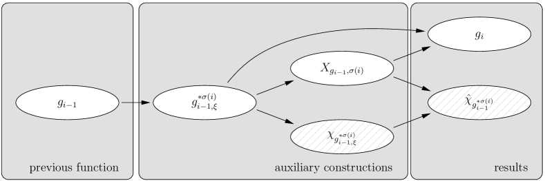
Figure 17: Illustration of the dependencies during the $i$-th replacement. The white-colored quantities are defined in Section 10.3 and the striped quantities in Section 10.4. Here “$\!A\to B$” means that $B$ is derived from $A$.

The definitions above are chosen such that the function $g_{i}$ exists. After the $k$-th step, the recursion ends with $g_{k}:{\Gamma\text{\rm-box}}\to\mathbb{R}_{\geq 0}$. We remark that, if we apply this mechanism to functions which are not admissible for controlled perturbation, the sequence of replacements will end-up with a function $g_{k}$ that fails the analysis from the next section.

Example 10

We get back to the 2-dimensional in_box-predicate. For this example it is sufficient to assume that the box is fixed somehow and that the only argument of the predicate is the query point $q=(x_{1},x_{2})$. This time we consider the various domains and critical sets of the functions $g_{i}$ that result from the sequence of replacements. (The order of the replacements is not important for this example.) The situation is illustrated in Figure 18. Picture (a) shows the domain (shaded region) of the function $f=g_{0}$ itself. We know that the critical set is the boundary of the query box.

After the replacement ${\text{\rm rep}}(g_{0},x_{1}\to\gamma_{1})$, the first argument belongs to the set $\pi_{1}({\Gamma\text{\rm-box}})$ resulting in an altered domain (see Picture (b)). We make two observations. Firstly, the critical set of $g_{1}$ is formed by two horizontal lines that are caused by the top and bottom part of the box $C_{g_{0}}$. What is the reason for that? If we consider the absolute value of $g_{0}$ while moving its argument along a horizontal line that passes through the top or bottom line segment of the box ($x_{2}$ is fixed then), it leads to a mapping that is zero on an open interval; in this case the mapping cannot be region-suitable. Secondly, there are no further contributions to the critical set of $g_{1}$. What is the reason? If we consider the absolute value of $g_{0}$ along a horizontal line that passes through the interior of the box, it leads to a mapping which is region-suitable.

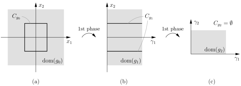
Figure 18: Illustration of the various domains and critical sets that result from the sequence of replacements for the 2-dimensional in_box-predicate.

Picture (c) shows the situation after the second replacement ${\text{\rm rep}}(g_{1},x_{2}\to\gamma_{2})$. The function $g_{2}$ is positive on its entire domain ${\Gamma\text{\rm-box}}$. The reason for this is that, if we consider the absolute value of $g_{1}$ along a vertical line ($\gamma_{1}$ is fixed then), it leads to a mapping which is region-suitable. $\bigcirc$

10.4 Derivation and Correctness of the Bounds

Although we have replaced each $x_{i}$ with $\gamma_{i}$ in the argument list of $f$ in a top-down manner, we are not able to determine the bounds $\nu_{f}$ and $\varphi_{f}$ in the same way. To achieve this goal, we need to go through the collected information bottom-up again. The reason is that, at the time we arrive at a function, say $g_{i-1}$, we cannot check directly if $g_{i-1}$ is region- and value-suitable. Instead of this, we want that these properties are inherited from the successor $g_{i}$ to the predecessor. We will see that, once we arrive at $g_{k}$, we can easily check if $g_{k}$ has the desired properties. This way we can possibly show that $g_{0}$, i.e. $f\!,$ is also region-value-suitable.

Therefore we divide the analysis in two phases. The first phase consists of the deduction of $g_{k}$ via the sequence of replacements and is already presented in the last section. The second phase consists of the deduction of the bounding functions $\varphi_{f}$ and $\chi_{f}$ and is the subject of this section. We begin with an auxiliary statement which claims that $g_{k}$ is non-decreasing in each argument under certain circumstances.

Lemma 8

Let ${(f,k,A,\delta,{e_{\text{\rm max}}},{\Gamma\text{\rm-box}},t)}$ be a predicate description where $A$ is an axis-parallel box without holes and let $I:=\{1,\ldots,k\}$. Let $\sigma:I\to I$ be bijective, i.e., an order on the elements of $I$. Finally, let $g_{0}:=f$ and $g_{j}:={\text{\rm rep}}(g_{j-1},x_{\sigma(j)}\to\gamma_{\sigma(j)})$ for all $1\leq j\leq k$, i.e., $g_{k}$ is the resulting function after the $k$ replacements. If the function $g_{k}$ is positive, it is non-decreasing in $\gamma_{i}$ on ${\pi_{i}}({\Gamma\text{\rm-box}})$ for all $i\in I$.

Proof

We refer to the explicit definition of $g_{i}$ in Formula (48) that reflects the replacement of the $i$-th argument: For growing $\gamma_{\sigma(i)}$ we shrink the domain for $x_{\sigma(i)}$ due to condition (C2). Formally, for $\gamma^{\prime},\gamma^{\prime\prime}\in\pi_{\sigma(i)}({\Gamma\text{\rm-box}})$ with $\gamma^{\prime}<\gamma^{\prime\prime}$ the corresponding regions of uncertainty are related in the way

$$R_{g_{i-1}^{*\sigma(i)},\gamma^{\prime}}(\bar{x}_{\sigma(i)})\;\subset\;R_{g_{i-1}^{*\sigma(i)},\gamma^{\prime\prime}}(\bar{x}_{\sigma(i)}).$$

Because the function value of $g_{i}$ is defined by the infimum absolute value, the function $g_{i}$ must be non-decreasing in its $i$-th argument $\gamma_{\sigma(i)}$ for region-regular $\xi$ by construction.

The same argumentation is true for each of the $k$ replacements and is independent of the actual sequence of replacements. This finishes the proof. ∎

The domain of the function $g_{k}$ is naturally ${\Gamma\text{\rm-box}}$. Even if ${\Gamma\text{\rm-box}}$ has the same cardinality than $\mathbb{R}$ for $k\geq 2$, it is non-obvious how to define an invertible function $\chi_{g_{k}}$ on ${\Gamma\text{\rm-box}}$. But such a bound is required to use the method of quantified relations. For that purpose we restrict the domain in the analysis to ${\Gamma\text{\rm-line}}$: It is true that the elements of $\gamma\in{\Gamma\text{\rm-line}}$ are now interlinked, but the important fact is that we can still choose them arbitrarily close to zero.

To further prepare the analysis, we have to focus on a peculiarity of the auxiliary function $g_{i-1,\xi}^{*\sigma(i)}$ for a given $i\in I$. Remember that $\nu_{g_{i-1,\xi}^{*\sigma(i)}}$ and $\chi_{g_{i-1,\xi}^{*\sigma(i)}}$ are families of functions with parameter $\xi\in{X}_{g_{i-1},\sigma(i)}$. Therefore we are facing the following issue: For a given $i\in I$, how can we deal with these two families of functions? The first solution that comes into mind is to replace each family with just one bounding function—so this is what we do. That means, we define the pointwise limits of these families as

$$\hat{\nu}_{g_{i-1}^{*\sigma(i)}}\left(\gamma_{\sigma(i)}\right) := \sup_{\xi\in{X}_{f,i}}\;\nu_{g_{i-1,\xi}^{*\sigma(i)}}\left(\gamma_{\sigma(i)}\right)$$

and

$$\hat{\chi}_{g_{i-1}^{*\sigma(i)}}\left(\gamma_{\sigma(i)}\right) := \inf_{\xi\in{X}_{f,i}}\;\chi_{g_{i-1,\xi}^{*\sigma(i)}}\left(\gamma_{\sigma(i)}\right)$$ (49)

for $\gamma\in{\Gamma\text{\rm-box}}$ and make use of these new bounds in the analysis. To illustrate this extra work in the analysis, we have added the two striped quantities in Figure 17.

Now we are ready to present the top-down approach to analyze real-valued functions. We claim and prove the results in the following theorem.

Theorem 10.1 (top-down approach)

Let ${(f,k,A,\delta,{e_{\text{\rm max}}},{\Gamma\text{\rm-box}},t)}$ be a predicate description where $A$ is an axis-parallel box without holes and let $I:=\{1,\ldots,k\}$. Let $\sigma:I\to I$ be bijective, i.e., an order on the elements of $I$. Finally, let $g_{0}:=f$ and $g_{j}:={\text{\rm rep}}(g_{j-1},x_{\sigma(j)}\to\gamma_{\sigma(j)})$ for all $1\leq j\leq k$. We define $\varphi_{f}$ and $\chi_{f}$ as

$$\varphi_{f}(\gamma) := g_{k}(\gamma)$$

$$\chi_{f}(\gamma) := \prod_{j=1}^{k}\,\hat{\chi}_{g_{j-1}^{*\sigma(j)}}\!\left(\gamma_{\sigma(j)}\right).$$

If $g_{k}$ is positive on $\,{\Gamma\text{\rm-box}}$ and $\chi_{f}$ is invertible on $\,{\Gamma\text{\rm-line}}$, then $f$ is region-value-suitable with the bounding functions $\varphi_{f}$ and $\chi_{f}$.

Proof

We prove the claim in three parts. First we show that there are certain bounding functions $\varphi_{g_{k}}$ and $\chi_{g_{k}}$ for which $g_{k}$ is region-value-suitable. Afterwards we prove that, if the function $g_{i}$ has such bounding functions, then $g_{i-1}$ has also appropriate bounding functions. And in the end we deduce the claim of the theorem.

Part 1 (basis). We assume that $g_{k}$ is positive on the open set $\,{\Gamma\text{\rm-box}}$, that means, we consider the function $g_{k}:{\Gamma\text{\rm-box}}\to\mathbb{R}_{>0}$. At first we decompose the domain in two parts (see Figure 19). Let $\gamma\in{\Gamma\text{\rm-line}}$. We define the unique open axis-parallel box with opposite vertices $\gamma$ and $\hat{\gamma}$ as

$${\Gamma\text{\rm-safe\,}_{\gamma}} := \left\{\gamma^{\prime}\in{\Gamma\text{\rm-box}}:\text{$\gamma_{i}\leq\gamma^{\prime}_{i}$ for all $i\in I$}\right\}\!.$$

We denote its complement within the ${\Gamma\text{\rm-box}}$ by

$${\Gamma\text{\rm-region\,}_{\gamma}} := {\Gamma\text{\rm-box}}\setminus{\Gamma\text{\rm-safe\,}_{\gamma}}.$$

We think of ${\Gamma\text{\rm-region\,}_{\gamma}}$ as the region of uncertainty and ${\Gamma\text{\rm-safe\,}_{\gamma}}$ as the region whose floating-point numbers are guaranteed to evaluate fp-safe.

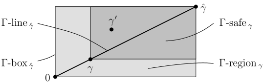
Figure 19: This is an exemplified 2-dimensional illustration of the decomposition of the ${\Gamma\text{\rm-box}}$ into the sets ${\Gamma\text{\rm-safe\,}_{\gamma}}$ and ${\Gamma\text{\rm-region\,}_{\gamma}}$ for $\gamma\in{\Gamma\text{\rm-line}}$.

We claim that $g_{k}$ is region-value-suitable on ${\Gamma\text{\rm-box}}$ in the following sense: We set the bounding functions to

$$\varphi_{g_{k}}(\gamma) := g_{k}(\gamma)$$

$$\chi_{g_{k}}(\gamma) := \prod_{j=1}^{k}\,\left(\hat{\gamma}_{j}-\gamma_{j}\right)$$

and claim that two statements are fulfilled for every $\gamma\in{\Gamma\text{\rm-line}}$:

1. The absolute value of $g_{k}(\gamma^{\prime})$ is at least $\varphi_{g_{k}}(\gamma)$ for all points $\gamma^{\prime}\in{\Gamma\text{\rm-safe\,}_{\gamma}}$.

2. The volume of ${\Gamma\text{\rm-safe\,}_{\gamma}}$ is $\chi_{g_{k}}(\gamma)$.

To prove the first statement, we consider the function value of $g_{k}$ along a path of $k$ axis-parallel line segments from $\gamma$ to $\gamma^{\prime}$. The path starts at $\gamma=(\gamma_{1},\ldots,\gamma_{k})$, connects the $(k-1)$ points $(\gamma^{\prime}_{1},\ldots,\gamma^{\prime}_{j},\gamma_{j+1}\ldots,\gamma_{k})$ with $1\leq j<k$ in ascending order of $j$ and ends at $\gamma^{\prime}=(\gamma^{\prime}_{1},\ldots,\gamma^{\prime}_{k})$. Along this path, the function value of $g_{k}$ is non-decreasing because of Lemma 8: For all $i\in I\!,$ the function $g_{k}$ is non-decreasing in its $i$-th argument $\gamma_{i}\in{\pi_{i}}({\Gamma\text{\rm-box}})$ for fixed $\xi\in{\pi_{\neq i}}({\Gamma\text{\rm-box}})$.

The proof of the second statement is straight forward: Because the box is axis-parallel, its volume is the product of its edge-lengths. We make the observation that the function $\chi_{g_{k}}(\gamma)$ is strictly monotonically increasing on ${\Gamma\text{\rm-line}}$ and hence must be invertible on this domain.

We conclude the first part of the proof: For a given $\gamma\in{\Gamma\text{\rm-line}}$, we have shown that the function value of $g_{k}$ is at least $\varphi_{g_{k}}(\gamma)$ on an area of volume $\chi_{g_{k}}(\gamma)$. This way we have found evidence that $g_{k}$ is region-value-suitable in the meaning above.

Part 2 (induction). We claim: For $i\in I$ and $\gamma\in{\Gamma\text{\rm-line}}$, the function value of $g_{i-1}$ is at least $\varphi_{g_{i-1}}(\gamma)$ on an area of volume $\chi_{g_{i-1}}(\gamma)$ with

$$\varphi_{g_{i-1}}(\gamma) := \varphi_{g_{i}}(\gamma)$$ (50)

$$\chi_{g_{i-1}}(\gamma) := \chi_{g_{i}}(\gamma)\,\cdot\,\frac{\hat{\chi}_{g_{i-1}^{*\sigma(i)}}\left(\gamma_{\sigma(i)}\right)}{\hat{\gamma}_{\sigma(i)}-\gamma_{\sigma(i)}}.$$ (51)

We prove the claim by mathematical induction for descending $i\in I$. Basis ($i=k$). Due to the first part, we can base the proof on the bounding functions $\varphi_{g_{k}}$ and $\chi_{g_{k}}$. Induction step ($i\in I$). We assume that the bounding functions are true for all $j\in I$ with $i\leq j\leq k$ and prove the claim for $i-1$. This is what we do next.

Remember the definition $g_{i}:={\text{\rm rep}}\!\left(g_{i-1},x_{\sigma(i)}\to\gamma_{\sigma(i)}\right)$. In the step backwards from $g_{i}$ to $g_{i-1}$, we observe the following difference in their two axis-parallel domains due to condition (C2) of Formula (48): The counterpart to the situation in which the $\sigma(i)$-th argument of $g_{i}$ lies in $\pi_{\sigma(i)}\left({\Gamma\text{\rm-safe\,}_{\gamma}}\right)$ is the situation in which the $\sigma(i)$-th argument of $g_{i-1}$ lies in

$$\bar{U}_{g^{*\sigma(i)}_{i-1,\delta_{\sigma(i)}}}\!\!\left(\bar{x}_{\sigma(i)}\right)\;\setminus\;R_{g^{*\sigma(i)}_{i-1,\gamma_{\sigma(i)}}}\!\!\left(\bar{x}_{\sigma(i)}\right)$$ (52)

and belongs to the region-regular case. Furthermore, the volume of this area is guaranteed to be at least $\hat{\chi}_{g^{*\sigma(i)}_{i-1}}\left(\gamma_{\sigma(i)}\right)$ due to Formula (49). Because the axis-parallel domains of $g_{i}$ and $g_{i-1}$ do not differ in directions different to the $\sigma(i)$-th main axis, their volume (which is the product of edge lengths) solely differ in a factor. Therefore we can estimate the volume $\chi_{g_{i-1}}(\gamma)$ at the product $\chi_{g_{i}}(\gamma)$ where we replace the factor $({\hat{\gamma}_{\sigma(i)}-\gamma_{\sigma(i)}})$ by $\hat{\chi}_{g_{i-1}^{*\sigma(i)}}\!(\gamma_{\sigma(i)})$; this validates Formula (51).

Because of Lemma 7, the lower-bounding function $\varphi_{g_{i}}$ is also a lower-bounding function on the volume of the area which is defined in Formula (52). This validates Formula (50).

Part 3 (conclusion). So far we have shown that for a given $\gamma\in{\Gamma\text{\rm-line}}$, the function value of $f=g_{0}$ is at least $\varphi_{f}(\gamma)$ on an area of volume $\chi_{f}(\gamma)$ because

$$\varphi_{f}(\gamma) = \varphi_{g_{0}}(\gamma)\;\;=\;\;\varphi_{g_{1}}(\gamma)\;\;=\;\;\cdots\;\;=\;\;\varphi_{g_{k}}(\gamma)\;\;=\;\;g_{k}(\gamma)$$

and because

$$\chi_{f}(\gamma) = \chi_{g_{0}}(\gamma)$$

$$= \chi_{g_{1}}(\gamma)\,\cdot\,\frac{\hat{\chi}_{g_{0}^{*\sigma(1)}}\left(\gamma_{\sigma(1)}\right)}{\hat{\gamma}_{\sigma(1)}-\gamma_{\sigma(1)}}$$

$$= \chi_{g_{2}}(\gamma)\,\cdot\,\frac{\hat{\chi}_{g_{1}^{*\sigma(2)}}\left(\gamma_{\sigma(2)}\right)}{\hat{\gamma}_{\sigma(2)}-\gamma_{\sigma(2)}}\,\cdot\,\frac{\hat{\chi}_{g_{0}^{*\sigma(1)}}\left(\gamma_{\sigma(1)}\right)}{\hat{\gamma}_{\sigma(1)}-\gamma_{\sigma(1)}}$$

$$\vdots$$

$$= \chi_{g_{k}}(\gamma)\,\cdot\,\prod_{i=1}^{k}\,\frac{\hat{\chi}_{g_{i-1}^{*\sigma(i)}}\left(\gamma_{\sigma(i)}\right)}{\hat{\gamma}_{\sigma(i)}-\gamma_{\sigma(i)}}$$

$$= \prod_{j=1}^{k}\,\left(\hat{\gamma}_{j}-\gamma_{j}\right)\,\cdot\,\prod_{i=1}^{k}\,\frac{\hat{\chi}_{g_{i-1}^{*\sigma(i)}}\left(\gamma_{\sigma(i)}\right)}{\hat{\gamma}_{\sigma(i)}-\gamma_{\sigma(i)}}$$

$$= \prod_{i=1}^{k}\,\left(\hat{\gamma}_{\sigma(i)}-\gamma_{\sigma(i)}\right)\,\cdot\,\prod_{i=1}^{k}\,\frac{\hat{\chi}_{g_{i-1}^{*\sigma(i)}}\left(\gamma_{\sigma(i)}\right)}{\hat{\gamma}_{\sigma(i)}-\gamma_{\sigma(i)}}$$

$$= \prod_{i=1}^{k}\,{\hat{\chi}_{g_{i-1}^{*\sigma(i)}}\left(\gamma_{\sigma(i)}\right)}.$$

If $\chi_{f}$ is in addition invertible on the domain $\,{\Gamma\text{\rm-line}}$, $f$ is region-value-suitable. This finishes the proof. ∎

One prerequisite in the last theorem is that $g_{k}$ is positive on the open ${\Gamma\text{\rm-box}}$. We make the observation that we cannot validate this property unless we have determined the entire sequence of replacements from $f=g_{0}$ down to $g_{k}$. That means, it is possible that the analysis fails at the end of the first phase.

Furthermore, we make the observation that the bounding functions $\varphi_{f}$ and $\chi_{f}$ are actually derived bottom-up in the the second phase of their derivation. That means, although we technically determine the sequence of functions $g_{i}$ in a top-down manner on the surface, the validity of the formulas is derived bottom-up afterwards. We summarize the steps of the top-down approach in Figure 20.

Figure 20: Instructions for performing the top-down approach. The illustration reflects the steps in which the quantities are determined according to Theorem 10.1.

10.5 Examples

Example 11

We use the top-down approach to determine the bounding functions $\varphi_{\text{\rm in\_box}}$ and $\chi_{\text{\rm in\_box}}$ for the predicate in_box. Again, we assume that the box is fixed somehow and that the only argument of the predicate is the query point. (There is no much influence on the analysis by the remaining parameters.) The predicate can be realized, for example, by the function

$$f(x) := \min_{1\leq i\leq k}\,\left\{\ell_{i}^{2}-(x_{i}-c_{i})^{2}\right\}$$

where $c\in\mathbb{R}^{k}$ is the center of the axis-parallel box and its edge lengths are given by $2\ell$. We eliminate the variables in ascending order from $x_{1}$ to $x_{k}$, that means, we set $\sigma(i):=i$ for all $1\leq i\leq k$.

Part 1 ($\varphi_{\text{\rm in\_box}}$). To determine $\varphi_{\text{\rm in\_box}}$ we need $g_{k}$, to determine $g_{k}$ we need the entire sequence of replacements, and to determine $g_{i}$ we need to determine the value of the “$\inf\inf$” expression in dependence on $\gamma_{i}$ in Formula (48). This is what we do next. Because of the symmetry of $f$, the following discussion is valid for all coordinates $x_{i}$.

To prepare the replacement of variables, we examine the function $f^{*i}$ for the region-regular case (see Figure 21).

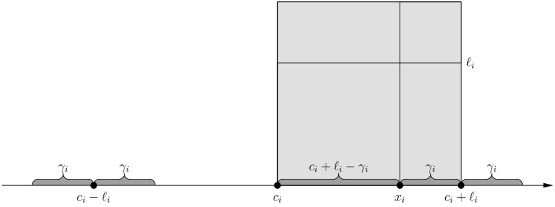
Figure 21: An illustration that supports the relation between the quantities of $f^{*i}$ for the region-regular case of the predicate in_box.

The critical set $C_{f^{*i}}$ contains two points, namely $c_{i}-\ell_{i}$ and $c_{i}+\ell_{i}$. By $\gamma_{i}$ we denote the minimal distance of $x_{i}$ to a point in $C_{f^{*i}}$. (Again we assume that $\hat{\gamma}_{i}$ must be less than $\ell_{i}$; otherwise the interior of the box would be covered entirely by the region of uncertainty and the predicate would lose its meaning.) The absolute value of $f$ grows in the distance to $C_{f^{*i}}$. To determine a guaranteed lower bound on the absolute value of $f$, we assume that the distance of $x_{i}$ to $C_{f^{*i}}$ is exactly $\gamma_{i}$. In addition we make the observation that $|f|$ grows slower towards the interior of the box than away from the box; therefore we must also assume that $x_{i}$ lies between $c_{i}-\ell_{i}$ and $c_{i}+\ell_{i}$ to get a convincing bound. This leads to the worst-case consideration $|x_{i}-c_{i}|=|c_{i}+\ell_{i}-\gamma_{i}|$. We make use of the binomial theorem to derive the unequation

$$\left|\ell_{i}^{2}-\left(x_{i}-c_{i}\right)^{2}\right| \geq \left|\ell_{i}^{2}-\left(c_{i}+\ell_{i}-\gamma_{i}\right)^{2}\right|$$

$$= \left|2\ell_{i}\gamma_{i}-\gamma_{i}^{2}\right|$$

$$= \left|\left(2\ell_{i}-\gamma_{i}\right)\gamma_{i}\right|.$$

Next we define the functions $g_{i}$ as

$$g_{i}(\gamma_{1},\ldots,\gamma_{i},x_{i+1},\ldots,x_{k}) := \min\;\Bigl{(}\!\!\begin{array}[t]{l}\bigl{\{}(2\ell_{j}-\gamma_{j})\gamma_{j}:1\leq j\leq i\bigr{\}}\\[4.30554pt] \cup\;\bigl{\{}\ell_{j}^{2}-\left(x_{j}-c_{j}\right)^{2}:i<j\leq k\bigr{\}}\Bigr{)}\end{array}$$

and in the end, the sequence of replacements leads to

$$\varphi_{\text{\rm in\_box}}(\gamma) := g_{k}(\gamma)$$

$$= \min_{1\leq j\leq k}\left(2\ell_{j}-\gamma_{j}\right)\gamma_{j}.$$

Part 2 ($\chi_{\text{\rm in\_box}}$). Now we determine a bound on the volume of the complement of the region of uncertainty. For every $i\in I$, a valid bounding function is given by

$$\hat{\chi}_{g^{*i}_{i-1}}\left(\gamma_{i}\right) = 2\delta_{i}-4\gamma_{i}.$$

This results in the following bound on the total volume:

$$\chi_{\text{\rm in\_box}}\left(\gamma\right) = \prod_{i=1}^{k}\,{\hat{\chi}_{g_{i-1}^{*i}}\left(\gamma_{i}\right)}$$

$$= \prod_{i=1}^{k}\left(2\delta_{i}-4\gamma_{i}\right).$$

Now that we have determined the bounding functions $\varphi_{\text{\rm in\_box}}$ and $\chi_{\text{\rm in\_box}}$, it would be possible to finish the analysis with the method of quantified relations—but this is not our interest in this section. $\bigcirc$

Example 12

This is the continuation of Examples 10 and 11. Here we want to investigate the regions of uncertainty for the various functions $g_{i}$. More precisely, we are interested in the correlation between the regions which are defined bottom-up in the second phase of the approach.

Figure 22 visualizes the regions of uncertainty for the functions $g_{i}$. The regions of uncertainty are light shaded whereas their complements are dark shaded. The decomposition is initiated by the choice of $\gamma\in{\Gamma\text{\rm-box}}$. Since each component $\gamma_{i}$ is positive, neighborhoods of the critical set are added to the region of uncertainty on the way back up to $g_{0}$.

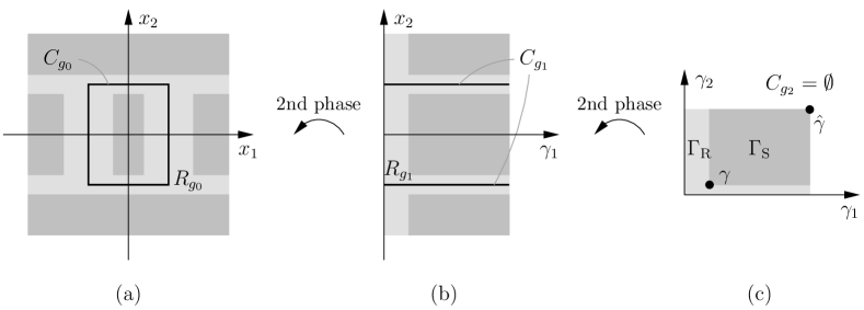
Figure 22: Illustration of the regions of uncertainty for the various domains in the analysis of the 2-dimensional in_box-predicate.

As we have seen in Example 10, the upper line segment of $C_{g_{0}}$ causes the upper line of $C_{g_{1}}$. Conversely, we can now see that the upper line of $C_{g_{1}}$ causes a region of uncertainty around the line which passes through the upper line segment of $C_{g_{0}}$. Be aware that our top-down approach is designed such that this behavior is forced for all non-region-regular situations. This implies that our method does not need any kind of exceptional sets. In the contrary, there are no restrictions on the measure of the critical sets at all: The only thing that matters is the criterion if $f$ is region-suitable or not. $\bigcirc$

10.6 Further Remarks

A different concept of the top-down approach is published in [46]. Although both presentations rest upon the same motivation, there are some technical differences in the realization. To avoid misunderstandings in the presentation and gain a deeper insight into our approach, we end this section with selected questions.

Does $f$ have to be (upper- or lower-) continuous to be top-down analyzable? No, we do not assume any kind of continuity in our approach. Points of discontinuity may be critical, but they do not have to be critical.

May we assume that $f$ is continuous? No, the top-down approach is defined recursively and the auxiliary functions $g_{i}$ are not continuous in general. Consider for example the continuous polynomial $f(x_{1},x_{2}):=x_{1}^{2}+x_{2}^{2}-1$ which is the planar “in unit circle” predicate. Then $g_{1}(x_{1},\gamma_{2})$ is not continuous in four points for fixed $\gamma_{2}$. The function is illustrated in Figure 23. That is the reason why the top-down approach must work for discontinuous functions.

Figure 23: Exemplified drawing of the “in unit circle” predicate after the first replacement. The function values on the interval $[-1,1]$ vary with $\gamma_{2}$.

Does a critical set of measure zero imply that $f$ is region-suitable? No, not in general. A notorious example is the density of $\mathbb{Q}$ in $\mathbb{R}$. Let $A\subset\mathbb{R}$ be an interval. Although $A\cap\mathbb{Q}$ is a set of measure zero, there is no $\varepsilon>0$ such that the neighborhood $U_{\varepsilon}(A\cap\mathbb{Q})$ has a volume smaller than $\mu(A)$. But the latter is a necessary criterion for region-suitability and the applicability of controlled perturbation.

Does region-suitability imply a finite critical set? No. A counter-example is the function $x\cdot\sin\left(\frac{1}{x}\right)$ which is region-suitable although it has infinitely many zeros in any finite neighborhood of zero. (By the way, this function is also value-suitable.) We summarize: Critical sets of region-suitable functions are countable, but not every countable critical set implies region-suitability.

Is it possible to neglect isolated points in the analysis? We may never exclude critical points from the analysis; they are always used to define the region of uncertainty. We may exclude less-critical points provided that we adjust the success-probability “by hand”. We may neglect non-critical points provided that we still determine the correct inf-value-suitable bound $\varphi_{\inf f}$. (See also Section 3.2.)

May we add additional points to the critical set? Yes, we may add points to the critical set provided that $f$ is still guaranteed to be region-suitable. (See also Section 3.2.)

Can we decide if $f$ is top-down analyzable without developing the sequence of replacements? It is a necessary condition for the top-down analyzability of $f$ that $g_{k}$ is positive everywhere. It is not clear how we can guarantee this property in general without deriving $g_{k}$.

11 Determining the Lower Fp-safety Bound

Here we introduce the design of guards and fp-safety bounds. Guards are necessary to implement guarded evaluations in ${\cal A}_{\text{\rm G}}$. In Section 11.1 we explain how guards can be implemented for a wide class of functions including polynomials. To analyze the behavior of guards, we introduce fp-safety bounds in Section 11.2. We explain how we determine the fp-safety bound in the analysis (see Figure 24). Furthermore, we prove the fp-safety bounds which we have used in previous sections.

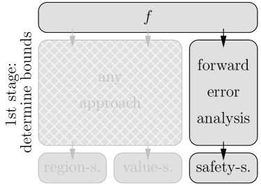
Figure 24: An error analysis is used to derive the bounding function for the safety-suitability in the first stage of the analysis.

11.1 Implementing Guarded Evaluations

Our presentation of guarded evaluations is based on rounding error analyses following the approach in [24, 7, 46]. A refinement is presented in the appendix of [46].

Rounding Error Analysis

The implementation of guards is based on maximum error bounds. To determine the error bounds we use rounding error analyses. Note that the error bound of a function $f$ depends on the formula $E$ that realizes $f$ and, especially, on the chosen sequence of evaluation. In Table 4 we cite some rules to determine error bounds. Expressions $E$ that are composed of addition, subtraction, multiplication and absolute value can be bounded by the value $B_{E}$ in the last row of the table. This includes the evaluation of polynomials; for further operators see [24, 7, 46]. The quantities $\text{\rm ind}_{E}$ and $\text{\rm sup}_{E}$ are derived according to the sequence of evaluation of $E$. The value $\text{\rm ind}_{x}$ is 0 if $x\in{\mathbb{F}_{L}}$, and it is 1 if $x$ is rounded.

Example 13

We determine the error bound for the expression

$$E(x_{1},\ldots x_{k})\!|_{\mathbb{F}} = (((a\cdot x_{1})\cdot x_{2})\cdots x_{k})\!|_{\mathbb{F}}$$

where $k\in\mathbb{N}$, $a\in\mathbb{R}$ is a coefficient and $x\in U_{\delta}(\bar{x})\!|_{\mathbb{G}}\subseteq[-2^{e_{\text{\rm max}}},2^{e_{\text{\rm max}}}]^{k}$. A worst-case consideration leads to $\text{\rm ind}_{a}=1$ and $\text{\rm sup}_{a}={\left|\,a\!|_{\mathbb{F}}\,\right|}$ for the coefficient and $\text{\rm ind}_{x_{i}}=0$ and $\text{\rm sup}_{x_{i}}={\left|\,x_{i}\!|_{\mathbb{F}}\,\right|}$ for $1\leq i\leq k$. Then we obtain $\text{\rm ind}_{ax_{1}}=2$ and $\text{\rm sup}_{ax_{1}}={\left|\,ax_{1}\!|_{\mathbb{F}}\,\right|}$ after the first multiplication. Taking all multiplications into account, we get $\text{\rm ind}_{E}=k+1$ and $\text{\rm sup}_{E}={\left|\,ax_{1}\cdots x_{k}\!|_{\mathbb{F}}\,\right|}$. According to Table 4 we obtain the dynamic error bound

$$B_{E}(L,x) = (k+1)\cdot{\left|\,ax_{1}\cdots x_{k}\!|_{\mathbb{F}}\,\right|}\cdot 2^{-L}$$

and the static error bound

$$B_{E}(L) = (k+1)\cdot{\left|\,a\!|_{\mathbb{F}}\,\right|}\cdot 2^{k{e_{\text{\rm max}}}-L}$$

where $2^{e_{\text{\rm max}}}$ is an upper bound on the absolute value of a perturbed input. $\bigcirc$

Remark 5

We make the important observation that the bound $B_{E}(L)$ approaches zero when $L$ approaches infinity, that means,

$$\lim_{L\to\infty}B_{E}(L) = 0.$$

Furthermore we observe that all error bounds which are derived from Table 4 have this property. $\bigcirc$

$$\begin{array}[]{|@{\qquad}c@{\qquad}|@{\qquad}c@{\qquad}|@{\qquad}c@{\qquad}|}\hline\cr\rule[-8.61108pt]{0.0pt}{21.52771pt}E&\text{\rm sup}_{E}&\text{\rm ind}_{E}\\ \hline\cr\hline\cr\rule[-8.61108pt]{0.0pt}{21.52771pt}x&{\left|\,x\,\!|_{\mathbb{F}}\,\right|}&\text{0 or 1}\\ \hline\cr\rule[-8.61108pt]{0.0pt}{21.52771pt}E_{1}\pm E_{2}&(\text{\rm sup}_{E_{1}}+\text{\rm sup}_{E_{2}})\!|_{\mathbb{F}}&1+\max\left\{\text{\rm ind}_{E_{1}},\text{\rm ind}_{E_{2}}\right\}\\ \hline\cr\rule[-8.61108pt]{0.0pt}{21.52771pt}E_{1}\cdot E_{2}&(\text{\rm sup}_{E_{1}}\cdot\text{\rm sup}_{E_{2}})\!|_{\mathbb{F}}&1+\text{\rm ind}_{E_{1}}+\text{\rm ind}_{E_{2}}\\ \hline\cr\rule[-8.61108pt]{0.0pt}{21.52771pt}|E|&\text{\rm sup}_{E}&\text{\rm ind}_{E}\\ \hline\cr\hline\cr\vrule\lx@intercol\hfil\rule[-8.61108pt]{0.0pt}{21.52771pt}B_{E}:=\text{\rm ind}_{E}\cdot\text{\rm sup}_{E}\cdot 2^{-L}\hfil\lx@intercol\vrule\lx@intercol\\ \hline\cr\end{array}$$

Table 4: This table reprints parts of Table 2.1 in Funke [24, p. 11]. The row for $|E|$ is added by us.

Guarded Evaluation

In guarded algorithms ${\cal A}_{\text{\rm G}}$ every predicate evaluation $f(x)\!|_{\mathbb{F}}$ must be protected by a guard ${\cal G}_{f}(x)$ that verifies the sign of the result. Guards can be implemented using the dynamic (or the weaker static) error bounds. Let $B_{f}(L,x)$ be an upper bound on the rounding error of $f(x)\!|_{\mathbb{F}}$ for floating point arithmetic ${\mathbb{F}_{L}}$, that means,

$$B_{f}(L,x) \geq {\left|\,f(x)\!|_{\mathbb{F}_{L}}-f(x)\,\right|}.$$ (55)

Then we can immediately derive the implication

$${\left|\,f(x)\!|_{\mathbb{F}}\,\right|}>B_{f}(L,x)\quad \Rightarrow \quad\text{\rm sign}(f(x)\!|_{\mathbb{F}_{L}})=\text{\rm sign}(f(x)).$$ (56)

We use the unequation on the left hand side to construct a guard ${\cal G}_{f}$ for $f$ where

$${\cal G}_{f}(x) := \big{(}\;{\left|\,f(x)\!|_{\mathbb{F}}\,\right|}>B_{f}(L,x)\,\big{)}.$$

If ${\cal G}_{f}(x)$ is true, $f(x)$ has the correct sign. Note that this definition is in accordance with Definition 2 on Page 2.

11.2 Analyzing Guards With Fp-safety Bounds

Now we explain how to analyze the behavior of guards according to [24, 7, 46]. Remember that we perform the analysis in real space. The implication

$${\left|\,f(x)\,\right|}>2B_{f}(L,x)\quad \Rightarrow \quad{\left|\,f(x)\!|_{\mathbb{F}}\,\right|}>B_{f}(L,x).$$ (57)

is true because of Formula (55). The inequality on the left hand side is a relation that we can safely verify in real space. We can always use the static error bound to construct a fp-safety bound $S_{\inf f}$ for $f$

$$S_{\inf f}(L) := 2B_{f}(L)$$

where $B_{f}(L)$ is the static error bound. Note that this definition is in accordance with Definition 6 on Page 6 because the implications in Formulas (56) and (57) guarantee the desired implication in Formula (8). Because of Remark 5, the fp-safety bound $S_{\inf f}(L)$ fulfills the safety-condition on page • ‣ 11 by construction. Next we derive a fp-safety bound for univariate polynomials.

Corollary 3

Let $f$ be a univariate polynomial

$$f(x) = a_{d}\cdot x^{d}+a_{d-1}\cdot x^{d-1}+\ldots+a_{1}\cdot x+a_{0}$$ (58)

of degree $d$. Then

$$S_{\inf f}(L) := (d+2)\cdot\max_{1\leq i\leq d}|a_{i}|\cdot 2^{{e_{\text{\rm max}}}(d+1)+1-L}$$ (59)

is a fp-safety bound for $f$ on $[-2^{e_{\text{\rm max}}},2^{e_{\text{\rm max}}}]$ where ${e_{\text{\rm max}}}\in\mathbb{N}$.

Proof

We apply the error analysis of this section. We evaluate Formula (58) from the right to the left. For a static error bound we get

$$B_{f}(L) := \text{\rm ind}_{f}\cdot\text{\rm sup}_{f}\cdot 2^{-L}\;\;=\;\;(d+2)\cdot\left(\max_{1\leq i\leq d}|a_{i}|\cdot 2^{{e_{\text{\rm max}}}(d+1)}\right)\cdot 2^{-L}.$$

Finally we set the fp-safety bound to $S_{\inf f}(L):=2B_{f}(L)$. ∎

Multiplications usually cause larger rounding errors than additions. Surprisingly, the evaluation of univariate polynomials with the Horner scheme (which minimize the number of multiplications) does not lead to a smaller error bound than the one we have derived in the proof. Next we derive an error bound for $k$-variate polynomials. We define $x^{\iota}:=x_{1}^{\iota_{1}}\cdot\ldots\cdot x_{k}^{\iota_{k}}$ for $\iota\in\mathbb{N}_{0}^{k}$ and $x\in\mathbb{R}^{k}$.

Corollary 4

Let $f$ be the $k$-variate polynomial ($k\geq 2$)

$$f(x) := \sum_{\iota\in{\cal I}}a_{\iota}x^{\iota}$$

where ${\cal I}\subset\mathbb{N}_{0}^{k}$ is finite and $a_{\iota}\in\mathbb{R}_{\neq 0}$ for all $\iota\in{\cal I}$. Let $d$ be the total degree of $f$ and let ${N_{\text{\rm T}}}$ be the number of terms in $f$. Then

$$S_{\inf f}(L) := (d+1+\lceil\log{N_{\text{\rm T}}}\rceil)\cdot{N_{\text{\rm T}}}\cdot\max_{\iota\in{\cal I}}|a_{\iota}|\cdot 2^{{e_{\text{\rm max}}}d+1-L}$$ (60)

is a fp-safety bound for $f$ on $[-2^{e_{\text{\rm max}}},2^{e_{\text{\rm max}}}]^{k}$ where ${e_{\text{\rm max}}}\in\mathbb{N}$.

Proof

We begin with the determination of the error bound $B_{f}$. The maximum absolute value of the term $a_{\iota}x^{\iota}$ is obviously upper-bounded by the product of a bound on $a_{\iota}$ and a bound on $x^{\iota}$. Because $|x_{i}|\leq 2^{e_{\text{\rm max}}}$ for all $1\leq i\leq k$ we have

$$\text{\rm sup}_{a_{\iota}x^{\iota}} \leq \max_{\iota\in{\cal I}}|a_{\iota}|\cdot 2^{{e_{\text{\rm max}}}d}.$$

Since we know the number ${N_{\text{\rm T}}}$ of terms in $f$​, we can then upper-bound $\text{\rm sup}_{f}$ by

$$\text{\rm sup}_{f} \leq {N_{\text{\rm T}}}\cdot\max_{\iota\in{\cal I}}|a_{\iota}|\cdot 2^{{e_{\text{\rm max}}}d}.$$

In addition, we have $\text{\rm ind}_{a_{\iota}x^{\iota}}=d+1$ since we evaluate $d$ multiplications and only $a_{\iota}$ may not be in the set $\mathbb{F}$. (Remember that, because of the perturbation, the values $x_{i}$ belong to the grid $\mathbb{G}$ which is a subset of $\mathbb{F}$.)

To keep $\text{\rm ind}_{f}$ as small as possible, we sum up the ${N_{\text{\rm T}}}$ terms pairwise such that the tree of evaluation has depth $\lceil\log{N_{\text{\rm T}}}\rceil$. This leads to $\text{\rm ind}_{f}=d+1+\lceil\log{N_{\text{\rm T}}}\rceil$. Therefore we conclude that

$$B_{f}(L) = \left(d+1+\lceil\log{N_{\text{\rm T}}}\rceil\right)\cdot\left({N_{\text{\rm T}}}\cdot\max_{\iota\in{\cal I}}|a_{\iota}|\cdot 2^{{e_{\text{\rm max}}}d}\right)\cdot 2^{-L}.$$

As usual we set $S_{\inf f}(L):=2B_{f}(L)$. ∎

12 The Treatment of Range Errors (All Components)

In this section we address a floating-point issue that is caused by poles of rational functions. So far the implementation and analysis of functions is based on the fact that signs of floating-point evaluations are only non-reliable on certain environments of zero. Now we argue that signs of evaluations may also be non-reliable on environments of poles. We do this for the purpose to embed rational functions into our theory. In Section 12.1 we extend the previous implementation considerations such that they can deal with range errors. In Section 12.2 we expand the analysis to range errors of the floating-point arithmetic $\mathbb{F}$. This is the first presentation that gains generality by the practical and theoretical treatment of range errors which, for example, are caused by poles of rational functions.

12.1 Extending the Implementation

We examine the simple rational function $f(x)=\frac{1}{x}$. It is well-known that the function value of $f$ at the pole $x=0$ does not exist in $\mathbb{R}$ (unless we introduce the unsigned symbolic value $\pm\infty$, see Forster [20]). We make the important observation that we cannot determine the function value of $f$ in a neighborhood of a pole with floating-point arithmetic ${\mathbb{F}_{L,K}}$ because the absolute value of $f$ may be too large. Moreover, we observe that the sign of $f$ may change on a neighborhood of a pole. Both observations suggest that poles play a similar role like zeros in the context of controlled perturbation. Now we extend the implementation such that it gets able to deal with range errors.

We extend the implementation of guarded evaluations in the following way: If the absolute value of $f$ cannot be represented with the floating-point arithmetic ${\mathbb{F}_{L,K}}$ because it is too large, we abort ${\cal A}_{\text{\rm G}}$ with the notification of a range error. We do not care about the source of the range error: It may be “division by zero” or “overflow.” The implementation of the second guard per evaluation is straight forward. Some programming languages provide an exception handling that can be used for this objective.

In addition we must change the implementation of the controlled perturbation algorithm ${\cal A}_{\text{\rm CP}}$. If ${\cal A}_{\text{\rm G}}$ fails because of a range error, we increase the bit length $K$ of the exponent (instead of the precision $L$). Be aware that we talk about the exponent, that means, an additive augmentation of the bit length implies a multiplicative augmentation of the range. These simple changes guarantee that the floating-point arithmetic ${\mathbb{F}_{L,K}}$ gets adjusted to the necessary dimensions in neighborhoods of poles or in regions where the function value is extremely large.

12.2 Extending the Analysis of Functions

For the purpose of dealing with range errors in the analysis, we need to adapt several parts of the analysis tool box. Below we present the necessary changes and extensions in the same order in which we have developed the theory.

Criticality and the region-suitability

The changes to deal with range errors affect the interface between the two stages of the analysis of functions. At first we extent the definition of criticality. We demand that certain points (e.g. poles of rational functions) are critical, too, and refine Definition 7 in the following way.

Definition 20 (critical)

Let ${(f,k,A,\delta,{e_{\text{\rm max}}})}$ be a predicate description. We call a point $c\in\bar{U}_{\delta}(\bar{x})$ critical if

$$\inf_{x\in U_{\varepsilon}(c)\setminus\{c\}}\;\left|f(x)\right|=0\quad \quad\sup_{x\in U_{\varepsilon}(c)\setminus\{c\}}\;\left|f(x)\right|=\infty$$ or

on a neighborhood $U_{\varepsilon}(c)$ for infinitesimal small $\varepsilon>0$. Furthermore, we call $c$ less-critical if $c$ is not critical, but $f(c)=0$ or $c$ is a pole. Points that are neither critical nor less-critical are called non-critical.

For simplicity and as before, we define the critical set $C_{f,\delta}$ to be the union of critical and less-critical points within $\bar{U}_{\delta}(\bar{x})$. Be aware that the new definition of criticality may expand the region of uncertainty. As a consequence it affects the region-suitability and the bound $\nu_{f}$, respectively $\chi_{f}$. Note that Definition 20 guarantees that we exclude neighborhoods of poles from now on. Because we have integrated poles into the definition of criticality, we have implicitly adapted the region-suitability.

The sup-value-suitability

So far we have only considered $\inf|f|$ outside of the region of uncertainty. But to get a quantified description of range issues in the analysis, we need to consider $\sup|f|$ as well. What we have called value-suitability so far is now called, more precisely, inf-value-suitability. Its bounding function, that we have called $\varphi_{f}(\gamma)$ so far, is now called $\varphi_{\inf f}(\gamma)$.

In addition to Definition 14 we introduce sup-value-suitability, that means, there is an upper-bounding function $\varphi_{\sup f}(\gamma)$ on the absolute value of $f$ outside of the region of uncertainty $R_{f}$. We show how the new bound is determined with the bottom-up approach later on. Based on the new terminology, we call $f$ (totally) value-suitable if $f$ is both: inf-value-suitable and sup-value-suitable.

The sup-safety-suitability and analyzability

We also extend Definition 15. What we have called safety-suitability so far is now called, more precisely, inf-safety-suitability. Its bounding function $S_{\inf f}(L)$ is now called the lower fp-safety bound.

In addition we introduce sup-safety-suitability, that means, there is an invertible upper-bounding function $S_{\sup f}(K)$ on the absolute value of $f$ with the following meaning: If we know that

$$|f(x)| \leq S_{\sup f}(K),$$

then $f(x)\!|_{\mathbb{F}}$ is definitely a finite number in ${\mathbb{F}_{L,K}}$. We call $S_{\sup f}(K)$ the upper fp-safety bound. Such a bound is trivially given by

$$S_{\sup f}(K) := 2^{2^{K-1}}-\,S_{\inf f}(L).$$

Based on the new terminology, we call $f$ (totally) safety-suitable if $f$ is both: inf-safety-suitable and sup-safety-suitable. As a consequence, we call $f$ analyzable if $f$ is region-suitable, value-suitable (both subtypes) and safety-suitable (both subtypes).

The method of quantified relations

Next we extent the method of quantified relations such that the new bounds on the range of floating-point arithmetic are included into the analysis. In addition to the precision function $L_{f}(p)$, we determine the bounding function

$$K_{f}(p) := \left\lceil S_{\sup f}^{-1}\left(\varphi_{\sup f}\left(t\cdot\nu_{f}^{-1}\left({\varepsilon_{\nu}\left(p\right)}\right)\right)\right)\right\rceil.$$

That means, we deduce the maximum absolute value of $f$ outside of the region of uncertainty from the probability; afterwards we use the upper fp-safety bound to deduce the necessary bit length of the exponent. The derivation of $K_{f}(p)$ is absolutely analog to the derivation of ${L_{\text{\rm safe}}}(p)$ in Steps 1–5 of the method of quantified relations.

We summarize our results so far: If we have the bounding functions of the interface of the function analysis, we know that the floating-point arithmetic $\mathbb{F}_{L_{f}(p),K_{f}(p)}$ is sufficient to safely evaluate $f$ at a random grid point in the perturbation area with probability $p$.

Furthermore, we can derive a probability function $p_{f}$ if $f$ is analyzable and $\varphi_{\inf f}$ and $\varphi_{\sup f}$ are both invertible. Analog to the definition of ${p_{\text{\rm inf}}}(L)$ in Remark 4.4, we derive the additional bound on the probability

$${p_{\text{\rm sup}}}(K) := \varepsilon_{\nu}^{-1}\left(\nu_{f}\left(\frac{1}{t}\cdot\varphi_{\sup f}^{-1}\left(S_{\sup f}(K)\right)\right)\right)$$

from $K_{f}(p)$. This leads to the final probability function $p_{f}:\mathbb{N}\times\mathbb{N}\to(0,1)$ where

$$p_{f}(L,K) := \min\left\{{p_{\text{\rm inf}}}(L),\,{p_{\text{\rm sup}}}(K),\,{p_{\text{\rm grid}}}(L)\right\}$$

for parameter $t\in(0,1)$.

The bottom-up approach

Now we extend the calculation rules of the bottom-up approach to also derive the bounding function $\varphi_{\sup f}(\gamma)$ from simpler sup-value-suitable functions. At first we replace the lower-bounding rule in Theorem 9.1 by the following sandwich-rule.

Theorem 12.1 (sandwich)

Let ${(f,k,A,\delta,{e_{\text{\rm max}}},{\Gamma\text{\rm-line}},t)}$ be a predicate description. If there is a region-value-suitable function $g:\bar{U}_{\delta}(A)\to\mathbb{R}$ and $c_{1},c_{2}\in\mathbb{R}_{>0}$ where

$$c_{1}\,|g(x)| \leq |f(x)|\;\;\leq\;\;c_{2}\,|g(x)|,$$

then $f$ is also region-value-suitable with the following bounding functions:

$$\nu_{f}(\gamma) := \nu_{g}(\gamma)$$

$$\varphi_{\inf f}(\gamma) := c_{1}\varphi_{\inf g}(\gamma)$$

$$\varphi_{\sup f}(\gamma) := c_{2}\varphi_{\sup g}(\gamma).$$

If $f$ is in addition safety-suitable, $f$ is analyzable.

Proof

The region-suitability and inf-value-suitability follows from the proof of Theorem 9.1. The sup-value-suitability is proven similar to Part 2 of the mentioned proof. ∎

Next we extent the product rule in Theorem 9.2. We just add the assignment

$$\varphi_{\sup f}(\gamma) := \varphi_{\sup g}(\gamma_{1},\ldots,\gamma_{\ell})\cdot\varphi_{\sup h}(\gamma_{j+1},\ldots,\gamma_{k}).$$

after Formula (33). Its proof follows Part 1 of the proof of Theorem 9.2.

At last we extent the min-rule and the max-rule in Theorem 9.3. We add the two assignments

$$\varphi_{\sup f_{\text{\rm min}}}(\gamma) := \min\{\varphi_{\sup g}(\gamma_{1},\ldots,\gamma_{\ell}),\varphi_{\sup h}(\gamma_{j+1},\ldots,\gamma_{k})\}$$

$$\varphi_{\sup f_{\text{\rm max}}}(\gamma) := \max\{\varphi_{\sup g}(\gamma_{1},\ldots,\gamma_{\ell}),\varphi_{\sup h}(\gamma_{j+1},\ldots,\gamma_{k})\}.$$

after Formula (38). Again, its proof follows Part 1 of the proof of Theorem 9.2.

The top-down approach

Similar to the functions $\varphi_{\inf g_{i}}$, which are simply called $\varphi_{g_{i}}$ in the overview in Figure 20, we determine the functions $\varphi_{\sup g_{i}}$ in the second phase of the pseudo-top-down approach in a bottom-up fashion.

This completes the integration of the range considerations into the analysis tool box. Be aware that all changes presented in this section do not restrict the applicability of the analysis tool box in any way. On the contrary, they are necessary for the correctness and generality of the tool box.

13 The Analysis of Rational Functions

We have just solved the arithmetical issues that occur in the implementation and analysis of rational functions. Besides we must solve technical issues in the implementation of guards and, moreover, provide a general technique to derive a quantitative analysis for rational functions. This is the first presentation that contains the implementation and analysis of rational functions.

Let $f:=\frac{g}{h}$ be a rational function, that means, let $g$ and $h$ be multivariate polynomials. Let $k$ be the number of arguments of $f$, i.e., we consider $f(x)$ where $x=(x_{1},\ldots,x_{k})$. The arguments of $g$ and $h$ may be any subsequence of $x$, but each $x_{i}$ is at least an argument of $g$ or an argument of $h$. We know that $g$ and $h$ are analyzable (see Section 9.5).

At first we discuss the implementation of guards for rational functions. We make the important observation that—independent of the evaluation sequences of $g$ and $h$—the division of the value of $g$ by the value of $h$ is the very last operation in the evaluation of $f$. Because of the standardization of floating-point arithmetic (e.g., see [33]), the sign of $f$ is computed correctly if the signs of $g$ and $h$ are computed correctly. Therefore it is sufficient for an implementation of a predicate that branches on the sign of a rational function $f$ to use the guard ${\cal G}_{f}:=\left({\cal G}_{g}\wedge{\cal G}_{h}\right)$.

But how do we analyze this predicate, that means, how can we relate the known quantities? Let $x$ be given. In the case that the (dependent) arguments of $g$ and $h$ lie outside of their region of uncertainty, we can deduce the relation

$$\frac{S_{\inf g}}{S_{\sup h}}\;\;\leq\;\;f(x)\;\;\leq\;\;\frac{S_{\sup g}}{S_{\inf h}}.$$ (61)

Unfortunately this is not what we need. This way, we can only deduce the value of $f$ from the values of $g$ and $h$, but not vice versa: If $f(x)$ fulfills Formula (61), we cannot deduce that the guards ${\cal G}_{g}$ and ${\cal G}_{h}$ are true. For example, assume that $f(x)=1$; then we know that the values of $g$ and $h$ are equal, but we do not know if their values are fp-safe or close to zero.

Therefore we choose a different way to analyze the behavior of guard ${\cal G}_{f}$. Since $g$ and $h$ are multivariate polynomials, we can analyze the behavior of ${\cal G}_{g}$ and ${\cal G}_{h}$ and derive the precision functions $L_{g}(p)$ and $L_{h}(p)$ as we have seen in earlier sections. If we demand that $g$ and $h$ evaluate successfully with probability $\frac{1+p}{2}$ each, $f$ evaluates successfully with probability $p$ since the sum of the failure probability of $g$ and $h$ is at most $(1-p)$. This leads to the precision function

$$L_{f}(p) := \max\left\{L_{g}\left(\frac{1+p}{2}\right),L_{h}\left(\frac{1+p}{2}\right)\right\}$$

which reflects the behavior of ${\cal G}_{f}$ and therefore analyzes the behavior of an implementation of the rational function evaluation of $f$.

14 General Analysis of Algorithms (Composition)

So far we have only presented components of the tool box which are used to analyze functions. Now we introduce the components which are used to analyze controlled-perturbation algorithms ${\cal A}_{\text{\rm CP}}$. Figure 25 illustrates the analysis of algorithms. Similar to the analysis of functions, the algorithm analysis has two stages. The interface between the stages is introduced in Section 14.1. It consists of necessary algorithm properties (to the left of the dashed line) and the analyzability of the used predicates (to the right of the dashed line). There we also show how to determine the bounds associated with the algorithm properties. In Section 14.2 we give an overview of algorithm properties. The method of distributed probability represents the actual analysis of algorithms and is presented in Section 14.3.

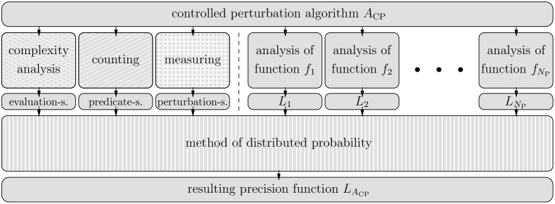
Figure 25: Illustration of the analysis of controlled-perturbation algorithms.

14.1 Necessary Conditions for the Analysis of Algorithms

Next we introduce several properties of controlled-perturbation algorithms. Sometimes we use the same names for algorithm and function properties to emphasize the analog. We describe to which algorithms we can apply controlled perturbation, for which we can verify that they terminate, and which we can analyze in a quantitative way because they are suitable for the analysis. In particular, three properties are necessary for the analyzability of algorithms: evaluation-, predicate- and perturbation-suitability. However, the three conditions are not sufficient for the analysis of algorithms since there are also prerequisites on the used predicates. In this section we define the various properties of controlled-perturbation algorithms, explain how we obtain the bounding functions that are associated with the necessary conditions, and show how the algorithm properties are related with each other.

Definition 21

Let ${\cal A}_{\text{\rm CP}}$ be a controlled perturbation algorithm.

• (applicable). We call ${\cal A}_{\text{\rm CP}}$ applicable if there is a precision function $L_{{\cal A}_{\text{\rm CP}}}:(0,1)\times\mathbb{N}\to\mathbb{N}$ and $\eta\in\mathbb{N}$ with the property: At least one from $\eta$ runs of the embedded guarded algorithm ${\cal A}_{\text{\rm G}}$ is expected to terminate successfully for a randomly perturbed input of size $n\in\mathbb{N}$ with probability at least $p\in(0,1)$ for every precision $L\in\mathbb{N}$ with $L\geq L_{{\cal A}_{\text{\rm CP}}}(p,n)$.

• (verifiable). We call ${\cal A}_{\text{\rm CP}}$ verifiable if the following conditions are fulfilled:
  1. All used predicates are verifiable.
  2. The perturbation area ${\cal U}_{{\cal A}_{\text{\rm CP}},\delta}(\bar{y})$ contains an open neighborhood of $\bar{y}$.
  3. The total number of predicate evaluations is bounded.
  4. The number of predicate types is bounded.

• (evaluation-suitable). We call ${\cal A}_{\text{\rm CP}}$ evaluation-suitable if the total number of predicate evaluations is upper-bounded by a function ${N_{\text{\rm E}}}:\mathbb{N}\to\mathbb{N}$ in dependence on the input size $n$.

• (predicate-suitable). We call ${\cal A}_{\text{\rm CP}}$ predicate-suitable if the number of different predicates is upper-bounded by a function ${N_{\text{\rm P}}}:\mathbb{N}\to\mathbb{N}$ in dependence on the input size $n$.

• (perturbation-suitable). Let ${\cal U}_{{\cal A}_{\text{\rm CP}},\delta}(\bar{y})$ be the perturbation area of ${\cal A}_{\text{\rm CP}}$ around $\bar{y}$; we assume that ${\cal U}_{{\cal A}_{\text{\rm CP}},\delta}(\bar{y})$ is scalable with parameter $\delta$ and that it has a fixed shape, e.g., cube, box, sphere, ellipsoid, etc. We call ${\cal A}_{\text{\rm CP}}$ perturbation-suitable if there is a bounding function $V\!:\mathbb{R}_{>0}^{k}\to\mathbb{R}_{>0}$ with the property that there is an open axis-parallel box $U_{{\cal A}_{\text{\rm CP}},\delta}(\bar{y})$ with volume at least $V(\delta)$ and $U_{{\cal A}_{\text{\rm CP}},\delta}(\bar{y})\subset{\cal U}_{{\cal A}_{\text{\rm CP}},\delta}(\bar{y})$.

• (analyzable). We call ${\cal A}_{\text{\rm CP}}$ analyzable if the following conditions are fulfilled:
  1. All used predicates are analyzable.
  2. ${\cal A}_{\text{\rm CP}}$ is evaluation-suitable, predicate-suitable and perturbation-suitable.

Remark 6

We add some remarks on the definitions above.

1. The applicability of an algorithm has a strong meaning: For every arbitrarily large success probability $p\in(0,1)$ and for every arbitrarily large input size $n\in\mathbb{N}$ there is still a finite precision that fulfills the requirements. As a matter of fact, a controlled perturbation algorithm reaches this precision after finite many steps. Because in addition the success probability is monotonically growing during the execution of ${\cal A}_{\text{\rm CP}}$, we conclude: If the algorithm ${\cal A}_{\text{\rm CP}}$ is applicable, its execution is guaranteed to terminate.

2. In the definition of applicability, we define the precision function $L_{{\cal A}_{\text{\rm CP}}}(p,n)$ as a function in the desired success probability $p$ and the input size $n$. Naturally, the bound also depends on other quantities like the perturbation parameter $\delta$, an upper bound on the absolute input values or the maximum rounding-error. However, the latter quantities have some influence in the determination of the bounding functions in the analysis of functions. Here they occur as parameters in formula $L_{{\cal A}_{\text{\rm CP}}}$ and are not mentioned as arguments.

3. We remark on the perturbation-suitability that we allow any shape of the perturbation area ${\cal U}_{{\cal A}_{\text{\rm CP}},\delta}$ in practice which fulfills the condition in the definition. As opposed to that we have assumed that the perturbation area $U_{f,\delta}$ in the analysis of functions is an axis-parallel box. This looks contradictorily and needs further explanation.

As a matter of fact, there is just one perturbation $y\in{\cal U}_{{\cal A}_{\text{\rm CP}},\delta}(\bar{y})\!|_{\mathbb{G}_{L,K}}$ of the input before we try to evaluate the whole sequence of predicates. We assume that the random perturbation is chosen from a discrete uniform distribution in a subset of the $n$-dimensional space. Opposed to that, function $f_{i}$ has just $k_{i}\ll n$ arguments $x=(x_{1},\ldots,x_{k_{i}})$. Mathematically speaking, we determine the input $x$ of $f_{i}$ by an orthogonal projection of $y$ onto a $k_{i}$-dimensional plane. Now we make the following important observation: If we examine the orthogonal projection onto a $k_{i}$-dimensional plane, the projected points do not occur with the same probability in general. We refer to Figure 26 and Figure 27. Despite of this observation, we prove in Section 14.3 that there is an implementation of ${\cal A}_{\text{\rm CP}}$ that we can analyze—presumed that we know the bounding function $V$ that is mentioned in the definition above.

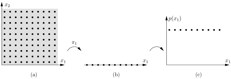
Figure 26: (a) The original perturbation area ${\cal U}_{{\cal A}_{\text{\rm CP}},\delta}$ is an axis-parallel box. (b) Its projection is uniformly distributed. (c) The points in the projection are chosen with the same probability.

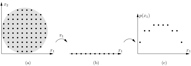
Figure 27: (a) The original perturbation area ${\cal U}_{{\cal A}_{\text{\rm CP}},\delta}$ is a sphere. (b) Its projection is uniformly distributed. (c) The points in the projection are not chosen with the same probability.

4. We remark on the predicate-suitability that the number ${N_{\text{\rm P}}}\in\mathbb{N}$ of different predicates is usually fixed for a geometric algorithm. Anyway, since we will see that the analysis can also be performed for a function ${N_{\text{\rm P}}}(n)$ we keep the presentation as general as possible. $\bigcirc$

Next we explain how we determine the three bounding functions which are associated with the three necessary algorithm properties. We refer to Figure 25. If the number ${N_{\text{\rm P}}}$ of used predicates is fixed, we just count them; otherwise we perform a complexity analysis to determine the bounding function ${N_{\text{\rm P}}}(n)$. We usually determine the bounding function ${N_{\text{\rm E}}}(n)$ on the number of predicate evaluations with a complexity analysis, too. The bound $\eta$ results from a geometric consideration: We only need to determine the real volume of the solid perturbation area. If the perturbation area has an ordinary shape, its computation is straight forward. We consider an example of this.

Example 14

Let the input of ${\cal A}_{\text{\rm CP}}$ be $m$ points in the plain, that means, $n=2m$. In addition let the perturbation area for each point be a disc of radius $\delta$. Then the axis-parallel square of maximum volume inside of such a disc has edge length $\delta\sqrt{2}$. We obtain:

$$\eta := \left\lceil\frac{\mu({\cal U}_{\delta})}{\mu(U_{\delta})}\right\rceil$$

$$= \left\lceil\frac{\mu(\text{$m$ discs of radius $\delta$})}{\mu(\text{$m$ cubes of edge length $\delta\sqrt{2}$})}\right\rceil$$

$$= \left\lceil\frac{m\cdot\pi\delta^{2}}{m\cdot 2\delta^{2}}\right\rceil$$

$$= 2$$

We observe that the bound $\eta$ does not depend on $m$ (or $n$). $\bigcirc$

Now we state and prove the implications of algorithm properties.

Lemma 9

Let algorithm ${\cal A}_{\text{\rm CP}}$ be analyzable. Then ${\cal A}_{\text{\rm CP}}$ is verifiable.

Proof

This is trivially true. ∎

Lemma 10

Let algorithm ${\cal A}_{\text{\rm CP}}$ be verifiable. Then ${\cal A}_{\text{\rm CP}}$ is applicable.

Proof

To show that ${\cal A}_{\text{\rm CP}}$ is applicable, we prove the following existence. There is $\eta\in\mathbb{N}$ such that for every $p\in(0,1)$ and every $n\in\mathbb{N}$ there is a precision ${{\cal L}_{p,n}}$ with the property: For a randomly perturbed input of size $n$, at least one from $\eta$ runs of ${\cal A}_{\text{\rm G}}$ is expected to terminate successfully with probability at least $p$ for every precision $L\in\mathbb{N}$ with $L\geq{{\cal L}_{p,n}}$. Then the function $L_{{\cal A}_{\text{\rm CP}}}(p,n):={{\cal L}_{p,n}}$ has the desired property which proves the claim.

At first we show that there is an appropriate $\eta\in\mathbb{N}$. Because ${\cal A}_{\text{\rm CP}}$ is verifiable, the perturbation area ${\cal U}_{{\cal A}_{\text{\rm CP}},\delta}(\bar{y})$ contains an open set around $\bar{y}$. Therefore there is an open axis-parallel box around $\bar{y}$ with $U_{\delta}(\bar{y})\subset{\cal U}_{{\cal A}_{\text{\rm CP}},\delta}(\bar{y})$. Then there is also a natural number

$$\eta := \left\lceil\frac{\mu\left({\cal U}_{{\cal A}_{\text{\rm CP}},\delta}(\bar{y})\right)}{\mu\left(U_{\delta}(\bar{y})\right)}\right\rceil.$$

That means, if we randomly choose $\eta$ points from a uniformly distributed grid in ${\cal U}_{{\cal A}_{\text{\rm CP}},\delta}(\bar{y})\!|_{\mathbb{G}_{L,K}}$, we may expect that at least one point lies also inside of $U_{\delta}(\bar{y})$.

Let $p\in(0,1)$ and let $n\in\mathbb{N}$. In addition let $y\in U_{\delta}(\bar{y})\!|_{\mathbb{G}_{L,K}}$ be randomly chosen. Since ${\cal A}_{\text{\rm CP}}$ is verifiable, there is an upper-bound ${N_{\text{\rm E}}}\in\mathbb{N}$ on the total number of predicate evaluations. Therefore we can distribute the total failure probability $(1-p)$ among the ${N_{\text{\rm E}}}$ predicate evaluations. Hence there is a probability

$$\varrho := \frac{1-p}{{N_{\text{\rm E}}}}.$$

Obviously ${\cal A}_{\text{\rm G}}(y)$ is successful with probability $p$ if every predicate evaluation fails with probability at most $\varrho$.

Let ${N_{\text{\rm P}}}\in\mathbb{N}$ be the number of different predicates in ${\cal A}_{\text{\rm G}}$ which are decided by the functions $f_{1},\ldots,f_{N_{\text{\rm P}}}$. Because ${\cal A}_{\text{\rm CP}}$ is verifiable, all used predicates are verifiable and thus applicable. Then Definition 10 implies the existence of precision functions $L_{f_{1}},\ldots,L_{f_{N_{\text{\rm P}}}}$. Therefore there is a precision

$${\cal L}_{p,n} := \max_{1\leq i\leq{N_{\text{\rm P}}}}\;L_{f_{i}}\left(1-\varrho\right)$$

which has the desired property because of Definition 10. This finishes the proof. ∎

As a consequence of Lemma 9 and Lemma 10 the controlled perturbation implementation ${\cal A}_{\text{\rm CP}}$ terminates with certainty and yields the correct result for the perturbed input if ${\cal A}_{\text{\rm CP}}$ is analyzable.

14.2 Overview: Algorithm Properties

An overview of the defined algorithm properties is shown in Figure 28. The meanings are: A controlled perturbation algorithm ${\cal A}_{\text{\rm CP}}$ is guaranteed to terminate if ${\cal A}_{\text{\rm CP}}$ is applicable (see Remark 6.1). If ${\cal A}_{\text{\rm CP}}$ is verifiable, we can prove that ${\cal A}_{\text{\rm CP}}$ terminates—even if we are not able to analyze its performance. And finally, we can give a quantitative analysis of the performance of ${\cal A}_{\text{\rm CP}}$ if ${\cal A}_{\text{\rm CP}}$ is analyzable.

The implications are: An evaluation-, perturbation- and predicate suitable algorithm that uses solely analyzable predicates is analyzable (see Definition 9). An analyzable algorithm is also verifiable (see Lemma 9). And a verifiable algorithm is also applicable (see Lemma 10).

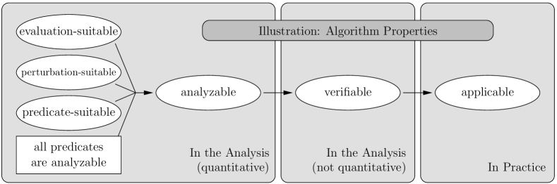
Figure 28: The illustration summarizes the implications of the various algorithm properties that we have defined in this section.

14.3 The Method of Distributed Probability

Here we state the main theorem of this section. The proof contains the method of distributed probability which is used to analyze complete algorithms. Figure 25 shows the component and its interface.

Theorem 14.1 (distributed probability)

Let ${\cal A}_{\text{\rm CP}}$ be analyzable. Then there is a general method to determine a precision function $L_{{\cal A}_{\text{\rm CP}}}:(0,1)\times\mathbb{N}\to\mathbb{N}$ and $K_{{\cal A}_{\text{\rm CP}}}:(0,1)\times\mathbb{N}\to\mathbb{N}$ and $\eta\in\mathbb{N}$ with the property: At least one from $\eta$ runs of the embedded guarded algorithm ${\cal A}_{\text{\rm G}}$ is expected to terminate successfully for a randomly perturbed input of size $n$ with probability at least $p\in(0,1)$ for every arithmetic ${\mathbb{F}_{L,K}}$ where $L\geq L_{{\cal A}_{\text{\rm CP}}}(p,n)$ and $K\geq K_{{\cal A}_{\text{\rm CP}}}(p,n)$.

Proof

We prove the claim in three steps: At first we derive $\eta\in\mathbb{N}$ from the shape of the region of uncertainty. Then we determine a bound on the failure probability of each predicate evaluation. And finally we analyze each predicate type to determine the worst-case precision. An overview of the steps is given in Table 5.

Step 1: determine “in axis-parallel box” probability (define $\eta$) Step 2: determine “per evaluation” probability (define $\rho$) Step 3: compose precision function (define $L_{{\cal A}_{\text{\rm CP}}}$ and $K_{{\cal A}_{\text{\rm CP}}}$)

Table 5: Instructions for performing the method of distributed probability.

Step 1 (define $\eta$). We define $\eta$ as the ratio

$$\eta = \left\lceil\frac{V(\delta)}{\mu(U_{\delta}(\bar{y}))}\right\rceil.$$

That means, if we randomly choose $\eta$ points from a uniformly distributed grid in ${\cal U}_{{\cal A}_{\text{\rm CP}},\delta}(\bar{y})\!|_{\mathbb{G}_{L,K}}$, we may expect that at least one point lies also inside of $U_{{\cal A}_{\text{\rm CP}},\delta}(\bar{y})$.

Step 2 (define $\rho$). Let $p\in(0,1)$ be the desired success probability of the guarded algorithm ${\cal A}_{\text{\rm G}}$. Then $(1-p)$ is the failure probability of ${\cal A}_{\text{\rm G}}$. There are at most ${N_{\text{\rm E}}}(n)$ predicate evaluations for an input of size $n$. That means, the guarded algorithm succeeds if and only if we evaluate all predicates successfully in a row for the same perturbed input. We observe that the evaluations do not have to be independent. Therefore we define the failure probability of each predicate evaluation as the function

$$\varrho(p,n) := \frac{1-p}{{N_{\text{\rm E}}}(n)}$$

in dependence on $p$ and $n$.

Step 3 (define $L_{{\cal A}_{\text{\rm CP}}}$ and $K_{{\cal A}_{\text{\rm CP}}}$). There are at most ${N_{\text{\rm P}}}(n)$ different predicates. Let $f_{1},\ldots,f_{{N_{\text{\rm P}}}(n)}$ be the functions that realize these predicates. Since all functions are analyzable, we determine their precision function $L_{f_{i}}$ with the presented methods of our analysis tool box. Then we define the precision function for the algorithm as

$$L_{{\cal A}_{\text{\rm CP}}}(p,n) := \max_{1\leq i\leq{N_{\text{\rm P}}}(n)}\;L_{f_{i}}(1-\varrho(p,n))$$

$$= \max_{1\leq i\leq{N_{\text{\rm P}}}(n)}\;L_{f_{i}}\left(1-\frac{1-p}{{N_{\text{\rm E}}}(n)}\right).$$

Analogically we define

$$K_{{\cal A}_{\text{\rm CP}}}(p,n) = \max_{1\leq i\leq{N_{\text{\rm P}}}(n)}\;K_{f_{i}}\left(1-\frac{1-p}{{N_{\text{\rm E}}}(n)}\right).$$

Then every arithmetic ${\mathbb{F}_{L,K}}$ with $L\geq L_{{\cal A}_{\text{\rm CP}}}(p,n)$ and $K\geq K_{{\cal A}_{\text{\rm CP}}}(p,n)$ has the desired property by construction. ∎

15 General Controlled Perturbation Implementations

We present a general way to implement controlled perturbation algorithms ${\cal A}_{\text{\rm CP}}$ to which we can apply our analysis tool box. The algorithm template is illustrated as Algorithm 2. It is important to see that all statements which are necessary for the controlled perturbation management are simply wrapped around the function call of ${\cal A}_{\text{\rm G}}$.

Algorithm 2 : ${\cal A}_{\text{\rm CP}}({\cal A}_{\text{\rm G}},\bar{y},{\cal U}_{\delta},\psi,\eta)$

  /* initialization */

  $L\leftarrow$ precision of built-in floating-point arithmetic

  $K\leftarrow$ exponent bit length of built-in floating-point arithmetic

  ${e_{\text{\rm max}}}\leftarrow$ determine upper bound $2^{e_{\text{\rm max}}}$ on $|\bar{y}_{i}|+\delta$

  repeat

     /* run guarded algorithm */

     for $i=1$ to $\eta$ do

        $y\leftarrow$ random point in ${\overline{\cal U}}_{\delta}(\bar{y})\!|_{\mathbb{G}_{L,K,{e_{\text{\rm max}}}}}$

        $\omega\leftarrow{\cal A}_{\text{\rm G}}(y,{\mathbb{F}_{L,K}})$

        if ${\cal A}_{\text{\rm G}}$ succeeded then

           leave the for-loop

        end if

     end for

     /* adjust parameters */

     if ${\cal A}_{\text{\rm G}}$ failed then

        if floating point overflow error occurred then

           /* guard failed because of range error */

           $K\leftarrow K+\psi_{K}$

        else

           /* guard failed because of insufficient precision */

           $L\leftarrow\lceil\psi_{L}\cdot L\rceil$

        end if

     end if

  until ${\cal A}_{\text{\rm G}}$ succeeded

  /* return perturbed input $y$ and result $\omega$ */

  return  $(y,\omega)$

Remember that the original perturbation area is ${\overline{\cal U}}_{\delta}(\bar{y})\!|_{\mathbb{G}}$. The implementation of a uniform perturbation seems to be a non-obvious task for most shapes. Therefore we propose axis-parallel perturbation areas in applications. (For example, we can replace spherical perturbation areas with cubes that are contained in them.) For axis-parallel areas there is the special bonus that the perturbation is composed of random integral numbers as we have explained in Remark 1.

An argument of the controlled perturbation implementation is the tuple $\psi=(\psi_{L},\psi_{K})\in\mathbb{R}\times\mathbb{N}$ of constants which are used for the augmentation of $L$ and $K$. The real constant $\psi_{L}>1$ is used for a multiplicative augmentation of $L$, and the natural number $\psi_{K}$ is used for an additive augmentation of $K$.

We remark that there is a variant of Algorithm 2 that also allows the increase of perturbation parameter $\delta$. Beginning with $\delta={\delta_{\text{\rm min}}}\in\mathbb{R}_{>0}^{k}$, we augment the perturbation parameter $\delta$ by a real factor $\psi_{\delta}>1$ each time we repeat the for-loop. When we leave the for-loop, we reset $\delta$ to ${\delta_{\text{\rm min}}}$. We observe that this strategy implies an upper-bound on the perturbation parameter by ${\delta_{\text{\rm max}}}:={\delta_{\text{\rm min}}}\cdot\psi_{\delta}^{\eta-1}$. This is the bound that we use in the analysis. To keep the presentation clear, we do not express variable perturbation parameters explicitly in the code.

A variable precision floating-point arithmetic is necessary for an implementation of ${\cal A}_{\text{\rm CP}}$. When we increase the precision in order to evaluate complex expressions successfully, the evaluation of simple expressions start suffering from the wasteful bits. Therefore we suggest floating-point filters as they are used in interval arithmetic. That means, we use a multi-precision arithmetic that refines the precision on demand up to the given $L$. If it is necessary to exceed $L$, ${\cal A}_{\text{\rm G}}$ fails. In the analysis we use this threshold on the precision.

16 Perturbation Policy

The meaning of perturbation is introduced in Section 3.1 and its implementation is explained in Remark 1 on Page 1. So far we have considered the original input to be the point $\bar{y}\in\mathbb{R}^{n}$ which is the concatenation of all coordinates of all input points for the geometric algorithm ${\cal A}_{\text{\rm CP}}$. In contrast to that, we now care for the geometric interpretation of the input and consider it as a sequence of geometric objects ${\cal O}_{1},\ldots,{\cal O}_{m}$. Then a perturbation of the input is the sequence of perturbed objects. In this section we define two different perturbation policies: The pointwise perturbation in Section 16.1 and the object-preserving perturbation in Section 16.2. The latter has the property that the topology of the input object is preserved. This is the first presentation that integrates object-preserving perturbations in the controlled-perturbation theory.

16.1 Pointwise Perturbation

For pointwise perturbations we assume that the geometric object is given by a sequence of points. A circle in the plain, for example, is given by three points. Another example is the polygon in Figure 29(a) which is represented by the sequence of four vertices $abcd$.

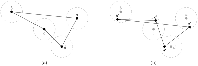
Figure 29: Example of a pointwise perturbation in the plane: (a) original input and (b) perturbed input.

The pointwise perturbation of a geometric object is the sequence of individually perturbed points of its description, i.e., randomly chosen points of their neighborhoods. Figure 29(b) shows a pointwise perturbed polygon $a^{\prime}b^{\prime}c^{\prime}d^{\prime}$ for our example. Because the perturbations are independent of each other, this policy is quite easy to implement. But we observe that pointwise perturbations do not preserve the structure of the input object in general: The original polygon $abcd$ is simple whereas the perturbed polygon $a^{\prime}b^{\prime}c^{\prime}d^{\prime}$ in our example is not. And the orientation of a circle that is defined by three perturbed points may differ from the orientation of the circle that is defined by the original points. Be aware that our analysis is particularly designed for pointwise perturbations. We suggest to apply this perturbation policy to inputs that are disturbed by nature, e.g., scanned data.

16.2 Object-preserving Perturbation

For object-preserving perturbations we assume that the geometric object is given by an anchor point and a sequence of fixed measurements. A circle in the plain, for example, is given by a center (anchor point) and a radius (fixed measurement). Another example is the polygon $abcd$ in Figure 30(a) which is given by an anchor point, say $a$, and implicitly by the sequence of vectors (the measurements) pointing from $a$ to $b$, from $a$ to $c$, and from $a$ to $d$.

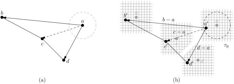
Figure 30: Example of an object-preserving perturbation in the plane: (a) original input and (b) perturbed input.

The object-preserving perturbation of a geometric object is a pointwise perturbation of its anchor point while maintaining all given measurements. Figure 30(b) shows polygon $a^{\prime}b^{\prime}c^{\prime}d^{\prime}$ that results from an object-preserving perturbation. There we have $b^{\prime}:=a^{\prime}+{b}-{a}$, etc. We observe that this perturbation is actually a translation of the object and hence preserves the structure of the input object in any respect: its orientation, measurements and angles. The object-preserving perturbation of a circle, for example, changes its location but not its radius.

The input must provide further information to support object-preserving perturbations. For the explicit representation, this policy requires a labeling of input values as anchor points (perturbable) or measurements (constant). For the implicit representation, the policy requires the subdivision of the input into single objects; then we make one of these points the anchor point and derive the measurements for the remaining points. To allow the object-preserving perturbation, the implementation must offer the labeling of values or the distinction of input objects.

In this context it is pleasant to observe that our perturbation area ${\overline{\cal U}}_{\delta}(A)\!|_{\mathbb{G}}$ supports object-preservation because it is composed of a regular grid. If the original object is represented without rounding error, the perturbed object is represented exactly as well. Of course, we can always apply object-preserving perturbations to finite-precision input objects. We suggest to apply this policy to inputs that result from computer-aided design (CAD): By design, the measurements are often multiples of a certain unit which can be used as an upper bound on the grid unit.

How can we analyze object-preserving perturbations? We consider the analysis of function $f$ that realizes a predicate. For pointwise perturbations we demand in Section 3.1 that $f$ only depends on input values. For object-preserving perturbations we only allow dependencies on anchor points: Every other point in the description of the object must be replaced in the formula by an expression that depends on the anchor point of the affected object. Be aware that these expressions can be resolved error-free due to the fixed-point grid $\mathbb{G}$. Then the new formula, depends only on anchor points (variables) and measurements (constants). The dependency of the function on the variables is analyzed as before. Finally we remark that we do not recommend perturbation policies that are based on scaling, stretching, sheering or rotation since the perturbed input cannot be represented error-free in general.

17 Appendix: List of Identifiers

Page numbers refer to definitions of the identifiers. References to preliminary definitions are parenthesized.

AlgorithmsPage

${\cal A}$

the given geometric algorithm ${\cal A}(\bar{y})$.

-

${\cal A}_{\text{\rm G}}$

the guarded version ${\cal A}_{\text{\rm G}}(y,{\mathbb{F}_{L,K}})$ of algorithm ${\cal A}$, i.e., all predicate evaluations are guarded.

3

${\cal A}_{\text{\rm CP}}$

the controlled perturbation version ${\cal A}_{\text{\rm CP}}({\cal A}_{\text{\rm G}},\bar{y},\delta,\psi)$ of algorithm ${\cal A}$. The implementation of ${\cal A}_{\text{\rm CP}}$ makes usage of ${\cal A}_{\text{\rm G}}$.

2

Sets and Number SystemsPage

$\mathbb{C}$

the set of complex numbers.

-

${\mathbb{F}_{L,K}}$

1. the set of floating point numbers with radix 2 whose precision has up to $L$ digits and whose exponent has up to $K$ digits.

2. the floating point arithmetic that is induced this way.

1

${\mathbb{G}_{L,K,{e_{\text{\rm max}}}}}$

the set of grid points. They are a certain subset of the floating point numbers ${\mathbb{F}_{L,K}}$ within the interval $[-2^{e_{\text{\rm max}}},2^{e_{\text{\rm max}}}]$.

5

$\mathbb{N}$; $\mathbb{N}_{0}$

the set of natural numbers; set of natural numbers including zero.

-

$\mathbb{Q}$

the set of rational numbers.

-

$\mathbb{R}$; $\mathbb{R}_{>0}$; $\mathbb{R}_{\neq 0}$

the set of real numbers; set of positive real numbers; set of real numbers excluding zero.

-

$\mathbb{Z}$

the set of integer numbers.

-

$X\!|_{\mathbb{F}_{L,K}}$

the restriction of a set $X$ to points in ${\mathbb{F}_{L,K}}$.

1

$X\!|_{\mathbb{G}_{L,K,{e_{\text{\rm max}}}}}$

the restriction of a set $X$ to points in ${\mathbb{G}_{L,K,{e_{\text{\rm max}}}}}$.

5

Identifiers of the AnalysisPage

$A$

the set of valid projected arguments $\bar{x}$ for $f$.

3.1

$B_{E}(L)$

a floating point error bound on the arithmetic expression $E$.

4

$C_{f}(\cdot)$

the critical set of $f$.

(7), 12

${\cal G}_{f}$

a guard for $f$ on the domain $X$.

2

$K$

the bit length of the exponent (see ${\mathbb{F}_{L,K}}$).

2.1

$K_{f}(p)$

a lower bound on the bit length of the exponent.

12

$L$

the bit length of the precision (see ${\mathbb{F}_{L,K}}$).

2.1

$L_{{\cal A}_{\text{\rm CP}}}(p,n)$

the precision function of ${\cal A}_{\text{\rm CP}}$.

• ‣ 21

$L_{f}(p)$

the precision function of $f$.

28

${L_{\text{\rm grid}}}$

a bound on the precision; caused by the grid unit condition.

(16), 27

${L_{\text{\rm safe}}}$

a bound on the precision; caused by the region- and safety-condition.

26

${N_{\text{\rm E}}}(n)$

an upper-bound on the number of predicate evaluations.

• ‣ 21

${N_{\text{\rm P}}}(n)$

an upper-bound on the number of different predicates.

• ‣ 21

$R_{f,\gamma}(\cdot)$

the region of uncertainty of $f$.

8

$R_{f,{\text{\rm aug}}(\gamma)}(\cdot)$

the augmented region of uncertainty of $f$.

3

$S_{\inf f}(L)$

the lower fp-safety bound.

6, (12)

$S_{\sup f}(K)$

the upper fp-safety bound.

12

$U_{f,\delta}(\cdot)$

the perturbation area of $f$; its shape is an axis-parallel box.

3.1

$U_{{\cal A}_{\text{\rm CP}},\delta}(\cdot)$

the perturbation area of ${\cal A}_{\text{\rm CP}}$; its shape is an axis-parallel box.

• ‣ 21

${\cal U}_{{\cal A}_{\text{\rm CP}},\delta}(\cdot)$

the perturbation area of ${\cal A}_{\text{\rm CP}}$; it may have any shape.

• ‣ 21

${e_{\text{\rm max}}}$

the input value parameter (see Formula (1)).

1

$f$

the real-valued function $f:\bar{U}_{\delta}(A)\to\mathbb{R}$ under consideration. We assume that the sign of $f$ decides a geometric predicate.

3.1

$k$

the arity of $f$.

3.1

$n$

the size of input $\bar{y}$.

3.1

$p_{f}(L,K)$

the probability function of $f$.

(4), 12

${p_{\text{\rm grid}}}(L)$

a bound on the probability; caused by the grid unit condition.

4

${p_{\text{\rm inf}}}(L)$

a bound on the probability; caused by the region- and inf-safety-condition.

4

${p_{\text{\rm sup}}}(K)$

a bound on the probability; caused by the sup-safety-condition.

12

$\text{\rm pr}(f\!|_{\mathbb{G}})$

the least probability that a guarded evaluation of $f$ is successful for inputs in $\mathbb{G}$ under the arithmetic $\mathbb{F}$.

7

$\frac{1}{t}$

the augmentation factor for the region of uncertainty.

5.1

$\bar{x}$

the arguments of $f$; projection of $\bar{y}$.

3.1

$x$

the perturbed arguments of $f$; projection of $y$.

3.1

$\bar{y}$

the original input to the algorithm.

3.1

$y$

the perturbed input $y\in U_{\delta}(\bar{y})$.

3.1

$\delta$

the perturbation parameter which bounds the maximum amount of perturbation componentwise.

3.1

$\gamma$

the tuple of componentwise distances to the critical set.

3

$\Gamma$

the set of valid augmented $\gamma$.

3

${\Gamma\text{\rm-box}}$

like $\Gamma$; the set is an axis parallel box.

3

${\Gamma\text{\rm-line}}$

like $\Gamma$; the set is a line.

3

$\nu_{f}(\gamma)$

an upper-bound on the volume of $R_{f,\gamma}$.

13

$\tau$

the grid unit.

5

$\varphi_{\inf f}(\gamma)$

a lower-bound on the absolute value of $f$ outside of $R_{f,\gamma}$.

14, (12)

$\varphi_{\sup f}(\gamma)$

an upper-bound on the absolute value of $f$ outside of $R_{f,\gamma}$.

12

$\chi_{f}(\gamma)$

a lower-bound on the complement of $\nu_{f}$ within the perturbation area.

19

$\psi$

the tuple $\psi=(\psi_{L},\psi_{K})\in\mathbb{R}\times\mathbb{N}$ is used for the augmentation of $L$ and $K$.

15

MiscellaneousPage

$\mu(\cdot)$

the Lebesgue measure.

3

$\pi(\cdot)$

the projection of points and sets, e.g., ${\pi_{i}}$, ${\pi_{<i}}$, ${\pi_{>i}}$, ${\pi_{\neq i}}$.

10.1

${\prec}$

the reverse lexicographic order.

9

${\prec}_{\sigma}$

the reverse lexicographic order after the permutation of the operands.

9

References

- [1] D. Avis, D. Bremner and R. Seidel. How Good Are Convex Hull Algorithms? In Computational Geometry: Theory and Applications, Vol. 7, pp. 265–301, 1997.
- [2] F. Avnaim, J.-D. Boissonnat, O. Devillers, F. P. Preparata and M. Yvinec. Evaluating Signs of Determinants Using Single-Precision Arithmetic. In Algorithmica, Vol. 17(2), pp. 111-132, 1997.
- [3] E. Berberich, A. Eigenwillig, M. Hemmer, S. Hert, L. Kettner, K. Mehlhorn, J. Reichelt, S. Schmitt, E. Schömer and Nicola Wolpert. EXACUS: Efficient and Exact Algorithms for Curves and Surfaces. In 13th Annual European Symposium on Algorithms, pp. 155–166, 2005.
- [4] M. de Berg, O. Cheong, M. van Kreveld and M. Overmars. Computational Geometry: Algorithms and Applications. Springer-Verlag, 3nd edition, 2008.
- [5] H. Brönnimann and M. Yvinec. Efficient Exact Evaluation of Signs of Determinants. In Algorithmica, Vol. 27(1), pp. 21–56, 2000.
- [6] Ch. Burnikel. Exact computation of Voronoi diagrams and line segment intersections. PhD Thesis, Max-Planck-Institut für Informatik, Universität des Saarlandes, 1996.
- [7] Ch. Burnikel, St. Funke, and M. Seel. Exact Geometric Computation Using Cascading. In International Journal of Computational Geometry and Applications, pp. 245–266, 2001; preliminary version Symposium on Computational Geometry, pp. 175–183, 1998.
- [8] Ch. Burnikel, K. Mehlhorn and St. Schirra. On Degeneracy in Geometric Computations. In Symposium on Discrete Algorithms, pp. 16–23, 1994.
- [9] M. Caroli. Evaluation of a Generic Method for Analyzing Controlled-Perturbation Algorithms. Master’s Thesis, Universität des Saarlandes, 2007.
-
[10]
Cgal - User and Reference Manual: All Parts.
Release 3.9, 2011.
http://www.cgal.org/Manual/latest/doc_pdf/cgal_manual.pdf - [11] T. H. Cormen and C. E. Leiserson and R. L. Rivest and C. Stein. Introduction to Algorithms. The MIT Press and McGraw-Hill, 1990.
- [12] O. Deiser. Einführung in die Mengenlehre. Springer-Verlag, 2. Auflage, 2004.
- [13] P. Deuflhard and A. Hohmann. Numerische Mathematik I: Eine algorithmisch orientierte Einführung. de Gruyter Lehrbuch, 3. Auflage, 2002.
- [14] H. Edelsbrunner and E. P. Mücke. Simulation of simplicity: A technique to cope with degenerate cases in geometric algorithms. In ACM Transactions on Graphics, Vol. 9(1), pp. 66–104, 1990.
- [15] I. Z. Emiris and J. F. Canny. A General Approach to Removing Degeneracies. In SIAM Journal on Computing, Vol. 24(3), pp. 650–664, 1995.
- [16] I. Z. Emiris, J. F. Canny and R. Seidel. Efficient Perturbations for Handling Geometric Degeneracies. In Algorithmica, Vol. 19(1), pp. 219–242, 1997.
- [17] Euklid von Alexandria. Die Elemente. Bücher I-XIII. Ostwalds Klassiker der Exakten Wissenschaften, Band 235. Verlag Harri Deutsch, 3. Auflage, 1997.
- [18] A. Fabri, G.-J. Giezeman, L. Kettner, St. Schirra and S. Schönherr. On the design of CGAL a computational geometry algorithms library Software Practice and Experience, Vol. 30(11), pp. 1167–1202.
- [19] W. Fischer and I. Lieb. Funktionentheorie – komplexe Analysis in einer Veränderlichen. Vieweg Studium, 9. Auflage, 2005.
- [20] O. Forster. Analysis 1: Differential- und Integralrechnung einer Veränderlichen. Vieweg-Verlag, 8. Auflage, 2006.
- [21] O. Forster. Analysis 3: Maß- und Integrationstheorie, Integralsätze im und Anwendungen. Vieweg+Teubner, 6. Auflage, 2011.
- [22] G. E. Forsythe. Pitfalls in Computation, or why a Math Book isn’t Enough. In The American Mathematical Monthly, Vol. 77(9), 931–956, 1970. Or in Technical Report No. CS 147, Computer Science Department, School of Humanities and Sciences, Stanford University, 1970.
- [23] S. Fortune and C. van Wyk. Static analysis yields efficient exact integer arithmetic for computational geometry. In ACM Transactions on Graphics, Vol. 15, pp. 223–248, 1996; preliminary version in 7th ACM Conference on Computational Geometry, pp. 163–172, 1993.
- [24] St. Funke. Exact Arithmetic using Cascaded Computation, Master’s Thesis, Universität des Saarlandes, 1997.
- [25] St. Funke, Ch. Klein, K. Mehlhorn, and S. Schmitt. Controlled perturbation for Delaunay triangulations. In Symposium on Discrete Algorithms, pp. 1047–1056, 2005.
- [26] D. Goldberg. What Every Computer Scientist Should Know About Floating-Point Arithmetic. In ACM Computing Surveys, Vol. 23(1), pp. 5–48, 1991.
- [27] P. Hachenberger and L. Kettner. Boolean operations on 3D selective Nef complexes: optimized implementation and experiments. In Symposium on Solid and Physical Modeling, pp. 163–174, 2005.
- [28] D. Halperin and E. Leiserowitz. Controlled perturbation for arrangements of circles. In International Journal of Computational Geometry and Applications, Vol. 14(4), pp. 277–310, 2004.
- [29] D. Halperin and S. Raab. Controlled perturbation for arrangements of polyhedral surfaces with application to swept volumes. In Symposium on Computational Geometry, pp. 163–172, 1999.
- [30] D. Halperin and Ch. R. Shelton. A perturbation scheme for spherical arrangements with application to molecular modeling. In Computational Geometry: Theory and Applications, Vol. 10, pp. 183–192, 1998.
- [31] M. Held. VRONI: An engineering approach to the reliable and efficient computation of Voronoi diagrams of points and line segments. In Computational Geometry: Theory and Applications, Vol. 18(2), pp. 95–123, 2001.
- [32] G. Hotz. Einführung in die Informatik. Leitfäden und Monographien der Informatik, Teubner, 1990.
- [33] IEEE Standard 754-2008 for Floating-Point Arithmetic. 2008.
- [34] T. Imai. A topology oriented algorithm for the Voronoi diagram of polygons. In Proceeding of the 8th Canadian Conference on Computational Geometry, Carleton University Press, Ottawa, Canada, pp. 107–112, 1996.
- [35] K. Jänich. Topologie. Springer-Verlag, 7. Auflage, 2001.
- [36] M. Jünger, G. Reinelt, and D. Zepf. Computing correct Delaunay triangulations. In Computing, Vol. 47, pp. 43–49, 1991.
- [37] M. Karasick, D. Lieber, and L.R. Nackman. Efficient Delaunay triangulation using rational arithmetic. In ACM Transactions on Graphics, Vol. 10(1), pp. 71–91, 1991.
- [38] L. Kettner, M. Mehlhorn, S. Pion, St. Schirra, and C.-K. Yap. Classroom Examples of Robustness Problems in Geometric Computations. In Computational Geometry: Theory and Applications, Vol. 40, pp. 702–713, 2008.
- [39] L. Kettner and St. Näher. Two Computational Geometry Libraries: LEDA and CGAL. In Jacob E. Goodman and Joseph O’Rourke, editors, Handbook of Discrete and Computational Geometry, second edition, pp. 1435-1463, 2004.
- [40] Ch. Klein. Controlled Perturbation for Voronoi Diagrams. Master’s Thesis, Universität des Saarlandes, 2004.
- [41] E. Lamprecht. Lineare Algebra I und II. Birkhäuser, 1993.
-
[42]
C. Li, C. Yap, S. Pion and Z. Du.
Core Library Tutorial.
Courant Institute of Mathematical Sciences, New York University, 2002.
http://www.cs.nyu.edu/exact/core/doc/tutorial.ps.gz - [43] K. Mehlhorn and S. Näher. The Implementation of Geometric Algorithms. In Proceedings of the 13th International Federation for Information Processing World Computer Congress, Vol. 1, pp. 223–231, Elsevier, 1994.
-
[44]
K. Mehlhorn and S. Näher.
The LEDA Platform for Combinatorial and Geometric Computing.
Cambridge University Press, 1999.
http://www.mpi-inf.mpg.de/mehlhorn/LEDAbook.html - [45] K. Mehlhorn, R. Osbild and M. Sagraloff. Reliable and Efficient Computational Geometry via Controlled Perturbation. In International Colloquium on Automata, Languages and Programming, Vol. 4051 of LNCS, pp. 299–310, 2006.
- [46] K. Mehlhorn, R. Osbild and M. Sagraloff. A General Approach to the Analysis of Controlled Perturbation Algorithms. In Computational Geometry: Theory and Applications, Vol. 44(9), pp. 507–528, 2011.
- [47] D. Michelucci. An epsilon-Arithmetic for Removing Degeneracies. In Proceedings of the 12th Symposium on Computer Arithmetic, pp. 230– 1995.
-
[48]
MPFI 1.0 - Multiple Precision Floating-Point Interval Library.
SPACES, INRIA Lorraine and Arenaire, INRIA Rhone-Alpes, 2002.
http://perso.ens-lyon.fr/nathalie.revol/mpfi_toc.html -
[49]
The MPFR team.
GNU MPFR - The Multiple Precision Floating-Point Reliable Library.
Edition 3.1.0, 2011.
http://www.mpfr.org/mpfr-current/mpfr.pdf - [50] M. Sagraloff and C.-K. Yap. A simple but exact and efficient algorithm for complex root isolation. In The International Symposium on Symbolic and Algebraic Computation, pp. 353–360, 2011.
- [51] M. Seel. An Accurate Arithmetic Implementation of Line Segment AVDs. Technical Report, Max-Planck-Institut für Informatik, 1996.
- [52] R. Seidel. The Nature and Meaning of Perturbations in Geometric Computing. In Discrete and Computational Geometry, Vol. 19(1), pp. 1–17, 1998.
- [53] J. R. Shewchuk. Adaptive Precision Floating-Point Arithmetic and Fast Robust Geometric Predicates. In Discrete and Computational Geometry, Vol. 18(3), pp. 305–368, 1997.
- [54] K. Sugihara and M. Iri. Construction of the Voronoi diagram for “one million” generators in single-precision arithmetic. In Proceedings of the IEEE, Vol. 80(9), pp. 1471–1484, 1992.
- [55] K. Sugihara, M. Iri, H. Inagaki and T. Imai. Topology-Oriented Implementation - An Approach to Robust Geometric Algorithms. In Algorithmica, Vol. 27(1), pp. 5–20, 2000.
- [56] C.-K. Yap. Geometric Consistency Theorem for a Symbolic Perturbation Scheme. In Journal of Computer and System Sciences, Vol. 40(1), pp. 2–18, 1990.
- [57] C.-K. Yap. Symbolic Treatment of Geometric Degeneration. In Journal of Symbolic Computation, Vol. 10(3), pp. 349–370, 1990.
- [58] C.-K. Yap. Towards exact geometric computation. In Computational Geometry: Theory and Applications, Vol. 7(1), pp. 3–23, 1997.