Dynamics and energetics for a molecular zipper model under external driving

Abstract

We investigate the dynamics of a single-ended $N$-state molecular zipper based on a model originally proposed by Kittel. The molecule is driven unidirectionally towards the completely unzipped state with increasing time $t$. The driving lowers the energies of states with $k$ unzipped links by an amount proportional to $kt$. We solve the Pauli rate equation for the state probabilities and the partial differential equations, which yield the probability distributions for the work performed on the zipper and for the heat exchanged with the thermal reservoir. Similarly to the related equilibrium model, two different regimes can be identified at a given temperature with respect to released molecular degrees of freedom per broken bond. In these two regimes the time evolution of the state probabilities as well as of the work and heat distributions show a qualitatively different behavior.

1 Introduction

The Watson-Crick double-stranded form represents the thermodynamically stable state of DNA in a wide range of temperature and salt conditions. However, even at standard physiologic conditions, there always exists possibility that the double-helix is locally unzipped into two strands both at its ends and in its interior [1, 2, 3, 4, 5]. If the interior unzipping is neglected, the unfolding of the two strands can be described by a simple zipper model [6, 7, 8]. This model, while including several simplifications, emphasizes the essential ingredient of the unzipping process, that means the competition between the entropic forces which tend to open the macromolecule, and the energetic forces that tend to condense it into its double-stranded form.

In the last two decades, new experimental techniques have been developed for detailed analysis of unzipping processes. A powerful technique are single molecule manipulations by optical tweezers [9, 10, 11, 12, 13, 14], where biomolecules are unfolded and refolded by applying mechanical forces. Because single molecules are subject to strong fluctuations, a stochastic description of the unfolding/refolding kinetics becomes necessary. Investigation of these stochastic processes can be useful to understand how biomolecules unfold and fold under locally applied forces [15, 16, 17, 18], as, for example, when mRNA passes through the ribosome during the translation process [19, 20], or when DNA is unzipped by helicase during the replication process [21, 22].

A particularly interesting part in the analysis of unzipping processes is the application of integral or detailed fluctuation theorems [23, 24, 25, 14, 26] to estimate free energy differences between folded and unfolded states (see, e.g., [27]). Their advantage is that they can be applied also to protocols, which drive the considered system far from equilibrium. It is thus not necessary to perform the unfolding/folding under quasi-static near-equilibrium conditions, where the process becomes reversible. Most popular theorems are the Crooks fluctuation theorem [28] and Jarzynski equality [29]. These relate to the distribution of work performed on the molecule during the process. Unfortunately it is not easy to get theoretical insight into characteristics of the underlying work distributions in far-from-equilibrium processes, since the work is a functional of the whole stochastic trajectory. Investigations have been conducted for simple spin systems driven by a time-dependent external field [30, 31, 32, 33, 34, 35] and for diffusion processes in the presence of a time-dependent potential [36, 37]. Analytical solutions are known for two-state systems [32, 33, 38, 35] and for systems with one continuous state variable [36, 37].

In this study we present analytical results for the work distribution for a multi-state system, which is motivated by a model proposed by Kittel for describing the melting transition of DNA molecules [8]. In order to derive analytical results, we had to consider a stochastic process with directed forwarded and forbidden backward transitions between states. As a consequence, detailed balance is broken and fluctuation theorems, as mentioned above, will not hold true. On the other hand, kinetic Monte Carlo simulations of the stochastic process show that, for at least certain parameter settings in the model, the restriction of forbidden backward transitions is not so severe and events dominating the integrand in the Jarzynski equality are not very rare. It is important to point out that these parameter settings are not related to any experimental conditions. In more realistic settings rare events would play the decisive role and in such cases it becomes difficult to determine tails of the work distribution with sufficient accuracy. Also the relation of the work considered in our study to the thermodynamic work measured in an unzipping experiments needs to be treated with care. These problems are discussed in detail in Sec. 2 and they imply that the theory cannot be applied to experiments at this stage. Our findings should nevertheless be useful because connection to experiments seems not completely out of reach and because they widen the range of hopping models, where analytical results for work distributions are available.

2 Unzipping in an extended Kittel model

Kittel’s model [8] is a simplified version of the Poland-Scheraga model [1] for the equilibrium properties of DNA molecules, which got renewed attention in the last ten years [39]. In contrast to the Poland-Scheraga model, it disregards the possibility of any interior openings (bubbles) of double-stranded parts of the molecule. Despite this simplification, it is already sufficient to understand the origin of a melting transition.

A molecule in Kittel’s model [8] has $N$ links in its fully folded state, see Fig. 1. Different states $k=1,\ldots,N$ of the molecule refer to configurations, where $(k-1)$ of the links are opened in a row. The difference $E_{k}-E_{1}$ of the internal energy of a state with $(k-1)$ open links and the ground state $k=1$ (no open links) is equal to $(k-1)\Delta$, corresponding to a loss of chemical bond energy $\Delta$ per broken link. With each broken link, the molecule gains $G$ degrees of freedom, which characterize the win of conformational degrees of freedom when double-stranded DNA is transferred to single stranded DNA. The entropy difference $S_{k}-S_{1}$ between the state $k$ and the ground state then becomes $k_{\rm B}\ln G^{k-1}=k_{\rm B}(k-1)\ln G$, where $k_{\rm B}$ is the Boltzmann constant. The free energy $F_{k}$ of state $k$ at a temperature $T$ is thus given by $F_{k}=F_{0}+(k-1)[\Delta-k_{\rm B}T\ln G]$ and the equilibrium properties can be readily worked out by considering the partition sum $Z=\sum_{k=1}^{N}\exp(-\beta F_{k})$, where $\beta=1/k_{\rm B}T$.

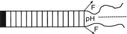
Figure 1: The zipper model.

In extending this model to treat unfolding kinetics, the molecule is supposed to unzip successively, one link in each step, as a consequence of a strong external driving. Such external driving can be caused by a local force or a pH gradient, as indicated in Fig. 1. With respect to pulling experiments on single DNA molecules out of equilibrium, there is evidence that a neglect of interior openings can become even less relevant than for the equilibrium properties. For example, far away from the melting temperature, e.g. at standard room temperature conditions (298 K), the unfolding kinetics of DNA hairpin molecules could be successfully described by assuming no interior openings and thermally activated unzipping transitions [16, 38]. Moreover, molecular fraying can be identified in individual unzipping trajectories by considering the size of force jumps. Thereby states with interior openings can be systematically excluded from the analysis [40].

We assume that the driving lowers the energy differences by an amount proportional to $(k-1)t$, i.e. open states with a larger number of broken links are favored with increasing time. If we take the ground state energy as the reference point, $E_{1}=0$, we obtain for the free energies $F_{k}(t)=E_{k}(t)-k_{\rm B}T\ln G^{k-1}$ of the states

$$F_{k}(t)=(k-1)[\Delta-vt-k_{\rm B}T\ln G]\,,\qquad k=1,\dots,N\,\,,$$ (1)

where the parameter $v$ has the dimension of an energy rate and characterizes different speeds of the unfolding in response to different strengths of the external driving.

Following established theoretical descriptions for the rupture kinetics of the bonds [38, 40, 41], the Kramers-Bell form [42] is used for the time-dependent transition rate $\lambda_{k,k+1}$ from state $k$ to state $(k+1)$,

$$\lambda_{k,k+1}(t)=\tilde{\nu}\exp[-\beta F_{k,k+1}(t)]\,.$$ (2)

Here $\tilde{\nu}$ is an attempt frequency and $F_{k,k+1}(t)$ denotes the free energy barrier for the transition, i.e. the difference of the free energy at the saddle point separating states $k$, $(k+1)$ and the free energy $F_{k}$ in state $k$. The barrier $F_{k,k+1}(t)$ is considered to be composed of a bare, $k$-independent free energy barrier, $F_{b}$, which is modified by an amount proportional to the free energy difference, $[F_{k+1}(t)-F_{k}(t)]$,

$$F_{k,k+1}(t)=F_{b}+\gamma[F_{k+1}(t)-F_{k}(t)]=F_{b}+\gamma[\Delta-vt-k_{\rm B}T\ln G]\,\,.$$ (3)

In the following we set $\gamma=1$ [43]. Note that $F_{k,k+1}(t)$ and thus $\lambda(t)\equiv\lambda_{k,k+1}(t)$ in Eq. (2) are independent of $k$. The attempt frequency $\tilde{\nu}$ in Eq. (2) was reported [44] to be approximately proportional to the ratio of the diffusion constant of the molecule in water to the water viscosity. We assume here a linear dependence of this ratio on the temperature $T$, i.e. we take $\tilde{\nu}=\nu(T/T_{0})$, where $\nu$ and $T_{0}$ are positive constants. Thus we obtain

$$\lambda(t)=\lambda_{k,k+1}(t)=g\exp[-\beta(d-vt)]\,\,,$$ (4)

where

$$g=\nu G\frac{T}{T_{0}}\,,\qquad d=\Delta+F_{b}\,.$$ (5)

If detailed balance is obeyed, i.e. $\lambda_{k,k+1}(t)\exp[-\beta F_{k}(t)]=\lambda_{k+1,k}(t)\exp[-\beta F_{k+1}(t)]$, the rates $\lambda_{k+1,k}(t)\equiv\lambda_{b}$ for backward (refolding) transitions become both independent of $k$ and $t$,

$$\lambda_{b}=\lambda_{k+1,k}(t)=\frac{g}{G}\exp(-\beta F_{b})\,\,.$$ (6)

Note that $G$ appears here in the denominator, which means that the ratio $\lambda_{b}/\lambda(t)=\exp(\beta\Delta-\beta vt)/G$ of backward to forward rates becomes small for large degeneracy factors $G$. This reflects the fact that it is difficult for the flexible unfolded part of the molecule to find proper configurations, which would allow for a reformation of (hydrogen) bonds.

If the model would refer to the hopping motion of a particle between time-dependent energy levels $E_{k}(t)$, the work performed on the system (for one realization of the stochastic process) would be

$$\mathsf{W}(t) = \int_{0}^{t}{\rm d}t^{\prime}\,\sum_{k=1}^{N}\dot{E}_{k}(t^{\prime})\delta_{k\mathsf{D}(t^{\prime})}$$ (7)

$$= [E_{\mathsf{D(t)}}(t)-E_{\mathsf{D(t)}}(t_{\mathsf{D(t)}})]+\sum_{k=1}^{\mathsf{D}(t)-1}[E_{k}(t_{k+1})-E_{k}(t_{k})]$$

$$= [F_{\mathsf{D(t)}}(t)-F_{\mathsf{D(t)}}(t_{\mathsf{D(t)}})]+\sum_{k=1}^{\mathsf{D}(t)-1}[F_{k}(t_{k+1})-F_{k}(t_{k})]\,\,,$$

where $\mathsf{D}(t)$ denotes the (random) state of the molecule at time $t$, $\dot{E}_{k}(t)={\rm d}E_{k}(t)/{\rm d}t$, and $t_{k}$ is the (random) time at which the transition from state $k$ to $(k+1)$ (rupture of $k$th bond) takes place ($t_{1}=0$ being the initial time). The last line in Eq. (7) follows from the fact that the entropy in the extended Kittel model is not dependent on time, i.e., for given $k$, differences between internal energies and between free energies at distinct times are equal.

The work in Eq. (7) can be related to the thermodynamic work $W_{f}$ in an unzipping experiment under force control. As pointed out in [45], work in thermodynamics is the internal energy transferred to a system upon changing the control parameters for given system configuration. This means that, when the force $f=f(t)$ is the control variable and the molecular extension $x$ the conjugate configurational variable, one has $W_{f}(t)=-\int_{f(0)}^{f(t)}{\rm d}fx$ [46]. Stochastic changes of the molecular extension occur mainly due to bond rupture, while in between transitions the response will be rather smooth and, under neglect of small thermal fluctuations, can be represented by a function $x(k,f)$. This specifies the mean end-to-end distance of the unfolded part in state $k$ at force $f$ (as often modeled by, e.g., the freely jointed or worm-like chain models from polymer physics). With $f_{k}\equiv f(t_{k})$ we then have

$$W_{f}(t)=-\int_{f(0)}^{f(t)}{\rm d}f\,x=-\int_{f_{\mathsf{D}(t)}}^{f(t)}{\rm d}f\,x(\mathsf{D}(t),f)-\sum_{k=1}^{\mathsf{D}(t)-1}\int_{f_{k}}^{f_{k+1}}{\rm d}f\,x(k,f)\,\,.$$ (8)

In more detailed energy landscape models, the free energy $F_{\rm tot}(k,f)$ of the molecule in state $k$ under loading $f$ can be represented as $F_{\rm tot}(k,f)=F_{0}(k)-fx(k,f)+F_{\rm str}(k,f)$ (see, e.g., [16]), where $F_{0}(k)$ is the free energy in the absence of loading and $F_{\rm str}(k,f)$ the elastic energy of the unfolded part upon stretching. For smooth response under stretching the latter is given by [16]

$$F_{\rm str}(k,f)=\int_{x(k,0)}^{x(k,f)}{\rm d}x\,\tilde{f}(k,x)=fx(k,f)-\int_{0}^{f}df^{\prime}\,x(k,f^{\prime})\,,$$ (9)

where $\tilde{f}(k,x)$ denotes the inverse function of $x(k,f)$ with respect to $f$. Accordingly, at a given $k$, the work for stretching upon increasing the force from $f_{a}$ to $f_{b}$ becomes

$$-\int_{f_{a}}^{f_{b}}df\,x(k,f) = F_{\rm str}(k,f_{b})-f_{b}x(k,f_{b})-F_{\rm str}(k,f_{a})+f_{a}x(k,f_{a})$$ (10)

$$= F_{\rm tot}(k,f_{b})-F_{\rm tot}(k,f_{a})\,\,.$$

This just means that the stretching at fixed $k$ is assumed to take place quasi-statically, i.e. the variation of the force is supposed to occur on a time scale much slower than the correlation time of end-to-end distance fluctuations. Inserting this result into Eq. (8) yields

$$W_{f}(t)=-[F_{\rm tot}(k,f(t))-F_{\rm tot}(k,\mathsf{D}(t))]-\sum_{k=1}^{\mathsf{D}(t)-1}[F_{\rm tot}(k,f(t_{k+1}))-F_{\rm tot}(k,f(t_{k}))]\,,$$ (11)

from which it becomes clear that $W_{f}$ equals $(-W)$, if $F_{\rm tot}(k,f(t))$ is identified with the free energy $F_{k}(t)$ in the extended Kittel model.

As said in the Introduction, we were able to find analytical results for the work distributions, if the backward rates in Eq. (6) were negligible. We are interested here in the model itself and will not make attempts to assign values to the parameters in the transition rates $\lambda(t)$ [Eq. (4)] and $\lambda_{b}$ [Eq. (6)], and appearing also in the state free energies in Eq. (1), which are connected to real experiments. Nevertheless, with respect to the value of the analytical results in connection with fluctuation theorems, the question arises whether a neglect of backward rates could be acceptable, at least for certain parameter settings. To check this, we have performed kinetic Monte Carlo simulations of the stochastic process. Because the forward rate from Eq. (4) can be written as $\lambda(t)=\lambda_{b}G\exp(-\beta\Delta+\beta vt)$ and the free energy differences appearing in Eq. (7) by $[F_{k}(t_{k+1})-F_{k}(t_{k})]=-(k-1)v(t_{k+1}-t_{k})$, the dynamics and energetics of the model is completely specified by the parameters $\lambda_{b}$, $G$, $v$, and $T$ (and $N$ if we consider a complete unfolding). For illustration and discussion of representative results, we here use $\Delta$, $\Delta/k_{\rm B}$, and $\nu^{-1}$ as units for energy, temperature and time, respectively.

Simulations were performed for fixed $N=10$, $T=1$ and $\lambda_{b}=1$, and a set of $v$ and $G$ values varying in the intervals $v=0.01-3.3$ and $G=10-1000$, respectively. We always started the unfolding from the fully closed state, i.e. $p_{k}(0)=\delta_{k,1}$ [47]. Probabilities $p_{N}(t)$ of complete unfolding (occupation of state $N$) until time $t$ were determined and an unfolding time $t_{U}$ defined by requiring that at $t=t_{U}$ the zipper has unfolded with a probability of 99.9%, i.e. $p_{N}(t_{U})=0.999$ (see Sec. 5). We then considered the work distributions $\rho(w,t_{U})$ at $t=t_{U}$ and the weighted distributions $\exp(-\beta w)\rho(w,t_{U})$, corresponding to the integrand in the average $\langle\exp(-\beta w)\rangle=\int{\rm d}w\,\exp(-\beta w)\rho(w,t_{U})$ as it appears in the Jarzynski equality. It was found that backward rates turn out to have a minor importance when the forward rates are much larger than the backward rates during the whole unfolding process or when $v$ is large enough. Specifically, the error in calculating $\langle\exp(-\beta w)\rangle$ is smaller than 5% when $v\gtrsim 3$ for $G=10$, $v\gtrsim 0.1$ for $G=100$, and $v\gtrsim 0.01$ for $G=1000$. As representative examples we show in Fig. 2 simulated results (blue lines) with nonzero backward rates in comparison with analytical results (green circles) for zero backward rates (see Sec. 4) for $p_{N}(t)$, $\rho(w,t_{U})$, and $\exp(-\beta w)\rho(w,t_{U})$, and parameters $v=0.25$, $G=10$ [panels labeled with a)] and $G=1000$ [panels labeled with b)]. As can be seen from the figure, for the case of large $G$ (small backward transitions), the simulated results for $\exp(-\beta w)\rho(w,t_{U})$ are almost indistinguishable from the analytical results.

The remaining part of the paper is organized as follows. In Sec. 3 we specify the equations for the time evolution of the state probabilities [Eq. (12)] and for the quantities describing the energy transformations [Eq. (17)]. In Sec. 4 we derive exact analytical solutions of these equations and in Sec. 5 we discuss our findings.

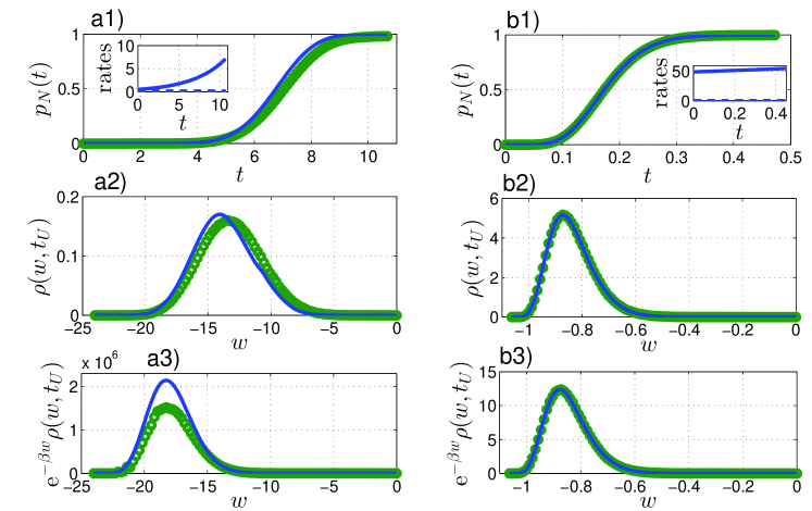
Figure 2: Simulated results of the model presented in Sec. 2 with backward transition rate $\lambda_{b}=0.133$ (blue lines) in comparison with analytical results (see Sec. 4) when neglecting backward transitions (green circles). Panels labeled with a) and b) refer to degeneracy factors $G=10$ and $G=1000$, respectively. The remaining parameters are $T=1$, $v=0.25$, and $N=10$. Panels a1) and b1) show the probability $p_{N}(t)$ that the zipper has unfolded up to time $t$ and the insets depict the time-dependence of the forward transition rates (full line); the constant backward rate is indicated by the dashed line. Panels a2) and b2) display the probability densities $\rho(w,t_{U})$ at the unfolding time $t_{U}$ ($t_{U}=10.67$ for $G=10$ and $t_{U}=0.47$ for $G=1000$), and panels a3) and b3) the weighted probability densities $\exp(-\beta w)\rho(w,t_{U})$.

3 Time evolution of state probabilities and work

Let $p_{k}(t)$, $k=1,\dots,N$, be the occupation probabilities of the $k$-th state. The time evolution of these functions is governed by the Pauli rate equation with transition rates given by Eq. (4). Formally speaking, the unzipping process is described by the time-inhomogeneous Markov process $\mathsf{D}(t)$, where $\mathsf{D}(t)=k$ if the system resides in state $k$ at time $t$. The Pauli rate equation can be written as

$$\frac{\mathrm{d}}{\mathrm{d}t}\mathbb{R}(t)=\mathbb{L}(t)\,\mathbb{R}(t)\,\,,\qquad\mathbb{R}(0)=\mathbb{I}\,\,,$$ (12)

where $\mathbb{I}$ is the $(N\times N)$ unity matrix, $\mathbb{L}(t)$ is the $(N\times N)$ matrix of the transition rates,

$$\mathbb{L}(t)=\left(\begin{array}[]{ccccc}-\lambda(t)&0&\dots&\dots&0\\ \lambda(t)&-\lambda(t)&\ddots&&\vdots\\ 0&\ddots&\ddots&\ddots&\vdots\\ \vdots&\ddots&\ddots&-\lambda(t)&0\\ 0&\dots&0&\lambda(t)&0\end{array}\right)\,\,,$$ (13)

and ${\mathbb{R}}(t)$ is the $(N\times N)$ matrix of the transition probabilities with the matrix elements

$$R_{ij}(t)={\rm Prob}\left\{\,\mathsf{D}(t)=i\,|\,\mathsf{D}(0)=j\,\right\}\,\,.$$ (14)

The matrix of transition probabilities evolves an arbitrary column vector of the initial occupation probabilities, $p(t)=\mathbb{R}(t)\,p(0)$. In the following, we always start with the completely closed zipper, that means $p_{k}(0)=\delta_{k1}$. The individual occupation probabilities then are

$$p_{i}(t)=R_{i1}(t)\,\,.$$ (15)

According to Eq. (7) the work $\mathsf{W}(t)$ is a functional of the process $\mathsf{D}(t)$. For an analytical treatment it is useful to introduce the augmented process $\left\{\mathsf{W}(t),\,\mathsf{D}(t)\right\}$ [49, 50, 33] which describes both the work and the state variable. This augmented process is again a time non-homogeneous Markov process and its one-time properties are described by $(N\times N)$ matrix ${\mathbb{G}}(w,t)$ with the matrix elements

$$G_{ij}(w,t)=\lim\limits_{\epsilon\to 0}\frac{{\rm Prob}\left\{\,\mathsf{W}(t)\in(w,w+\epsilon)\,{\rm and}\,\mathsf{D}(t)=i\,|\,\mathsf{W}(0)=0\,{\rm and}\,\mathsf{D}(0)=j\,\right\}}{\epsilon}\,\,.$$ (16)

The time evolution of ${\mathbb{G}}(w,t)$ is given by [49, 50, 33]

$$\frac{\partial}{\partial t}{\mathbb{G}}(w,t)=\left[-\frac{\partial}{\partial w}\,\,\dot{{\mathbb{E}}}(t)+\mathbb{L}(t)\,\right]\,{\mathbb{G}}(w,t)\,\,,\qquad{\mathbb{G}}(w,0)=\delta(w)\,{\mathbb{I}}\,\,.$$ (17)

Here $\dot{{\mathbb{E}}}(t)$ is the diagonal matrix $\dot{{\mathbb{E}}}(t)={\rm diag}\{\dot{E}_{1}(t),\dots,\dot{E}_{N}(t)\}$. Notice that ${\mathbb{R}}(t)=\int_{-\infty}^{\infty}{\rm d}w\,{\mathbb{G}}(w,t)$. Eq. (17) represents a hyperbolic system of $N^{2}$ coupled partial differential equations with time-dependent coefficients. Its exact solution will be given in the following Sec. 4.

The matrix ${\mathbb{G}}(w,t)$ provides a complete description of the energetics of the unzipping process. The joint probability density for the internal energy $\mathsf{U}(t)=E_{\mathsf{D}(t)}(t)$ and the work $\mathsf{W}(t)$ performed on the system during the time interval $[0,t]$ (regardless of the final state of the system at the time $t$) is given by

$$\xi(u,w,t)=\sum_{i=1}^{N}\,\delta\left[u-E_{i}(t)\right]\,G_{i1}(w,t)\,\,,$$ (18)

where $\delta(x)$ is the Dirac $\delta$-function. The last function already yields the probability density for the work,

$$\rho(w,t)=\int_{-\infty}^{\infty}{\rm d}u\,\,\xi(u,w,t)\,\,.$$ (19)

An analogous integration over the work variable $w$ gives the probability density of $\mathsf{U}(t)$. Furthermore, the first law of thermodynamics implies $\mathsf{U}(t)-\mathsf{U}(0)=\mathsf{U}(t)=\mathsf{W}(t)+\mathsf{Q}(t)$ (note that $\mathsf{U}(0)=0$ for our setting) and, accordingly, $\xi(u,w,t)$ gives also the probability density of the heat $\mathsf{Q}(t)$ transferred from the reservoir during the time interval $[0,t]$ [35].

The mean values of the internal energy, work and heat, are then

$$\rule[-4.30554pt]{0.0pt}{25.83325pt}U(t) = \int_{-\infty}^{\infty}\int_{-\infty}^{\infty}{\rm d}u\,{\rm d}w\,u\,\xi(u,w,t)=\sum_{i=1}^{N}E_{i}(t)p_{i}(t)\,\,,$$ (20)

$$\rule[-4.30554pt]{0.0pt}{25.83325pt}W(t) = \int_{-\infty}^{\infty}\int_{-\infty}^{\infty}{\rm d}u\,{\rm d}w\,w\,\xi(u,w,t)=\sum_{i=1}^{N}\int_{0}^{t}{\rm d}t\,\dot{E}_{i}(t)p_{i}(t)\,\,,$$ (21)

$$\rule[-4.30554pt]{0.0pt}{25.83325pt}Q(t) = \int_{-\infty}^{\infty}\int_{-\infty}^{\infty}{\rm d}u\,{\rm d}w\,(u-w)\,\xi(u,w,t)=\sum_{i=1}^{N}\int_{0}^{t}{\rm d}t\,E_{i}(t)\dot{p}_{i}(t)\,\,.$$ (22)

Notice that these mean values can be also calculated directly from the solution of the Pauli rate equation (12). However, for higher moments, we already need the function $\xi(u,w,t)$. For example, the variances discussed in Sec. 5 are given by

$$\rule[-4.30554pt]{0.0pt}{25.83325pt}[\Delta U(t)]^{2} = \int_{-\infty}^{\infty}\int_{-\infty}^{\infty}{\rm d}u\,{\rm d}w\,u^{2}\,\xi(u,w,t)-[U(t)]^{2}\,\,,$$ (23)

$$\rule[-4.30554pt]{0.0pt}{25.83325pt}[\Delta W(t)]^{2} = \int_{-\infty}^{\infty}\int_{-\infty}^{\infty}{\rm d}u\,{\rm d}w\,w^{2}\,\xi(u,w,t)-[W(t)]^{2}\,\,,$$ (24)

$$\rule[-4.30554pt]{0.0pt}{25.83325pt}[\Delta Q(t)]^{2} = \int_{-\infty}^{\infty}\int_{-\infty}^{\infty}{\rm d}u\,{\rm d}w\,(u-w)^{2}\,\xi(u,w,t)-[Q(t)]^{2}\,\,.$$ (25)

4 Solution of the model

Owing to the simple two-diagonal structure of the matrix $\mathbb{L}(t)$ in Eq. (13), the system (12) can be solved by simple integrations. By defining

$$\Lambda(t,t^{\prime})=\int_{t^{\prime}}^{t}\,{\rm d}t^{\prime\prime}\lambda(t^{\prime\prime})=\frac{\alpha}{\beta v}\left[\exp(\beta vt)-\exp(\beta vt^{\prime})\right]\,\,,$$ (26)

where $\alpha=g\exp(-\beta d)$, a recursive treatment of Eq. (12) yields

$$\begin{array}[]{lc}\rule[-4.30554pt]{0.0pt}{25.83325pt}R_{ij}(t)=0\,\,,&\quad i<j\,\,,\\ \rule[-4.30554pt]{0.0pt}{25.83325pt}R_{jj}(t)=\exp{\left[-\Lambda(t,0)\right]}\,\,,&\quad j=1,\ldots,N\,\,,\\ \rule[-4.30554pt]{0.0pt}{25.83325pt}R_{ij}(t)=\displaystyle{\int_{0}^{t}}\,{\rm d}t^{\prime}\exp{\left[-\Lambda(t,t^{\prime})\right]}\,\lambda(t^{\prime})\,R_{i-1j}(t^{\prime})\,\,,&\quad j<i<N\,\,,\\ \rule[-4.30554pt]{0.0pt}{25.83325pt}R_{Nj}(t)=\displaystyle{\int_{0}^{t}}\,{\rm d}t^{\prime}\lambda(t^{\prime})\,R_{N-1j}(t^{\prime})\,\,,&\quad j=1,\ldots,N\,\,.\end{array}$$ (31)

When solving these recursive relations, we obtain the lower triangular matrix with the nonzero matrix elements

$$\rule[-4.30554pt]{0.0pt}{25.83325pt}R_{j+kj}(t) = \frac{\left[\Lambda(t,0)\right]^{k}}{k!}\,\exp\left[-\Lambda(t,0)\right]\,\,,\,\,\quad j=1,\ldots,N-1\,\,;\,\,k=0,\dots,N-1-j\,\,,$$ (32)

$$\rule[-4.30554pt]{0.0pt}{25.83325pt}R_{Nj}(t) = \frac{\left[\Lambda(t,0)\right]^{N-j}}{(N-j)!}\,\exp\left[-\Lambda(t,0)\right]\,{}_{1}\!F_{1}(1,N+1-j;\Lambda(t,0))\,\,,\,\,\quad j=1,\ldots,N\,\,.$$ (33)

where ${}_{1}\!F_{1}(a,b;x)$ denotes the confluent hypergeometric function.

For solving Eq. (17) we first perform a Laplace transform with respect to the work variable $w$. To keep the notation simple, we use the same symbols for the original functions and for the transformed ones. The transformed functions will be distinguished by explicitly giving the complex variable $s$ conjugate to $w$. After performing the Laplace transformation, we get the system of ordinary differential equations

$$\frac{\partial}{\partial t}{\mathbb{G}}(s,t)=\left[-s\,\dot{{\mathbb{E}}}(t)+\mathbb{L}(t)\,\right]\,{\mathbb{G}}(s,t)\,\,,\qquad{\mathbb{G}}(s,0)={\mathbb{I}}\,\,.$$ (34)

The matrix which multiplies ${\mathbb{G}}(s,t)$ on the right hand side is again a lower two-diagonal one. Therefore, similarly to Eq. (31), we find the recursive relation

$$\begin{array}[]{lc}\rule[-4.30554pt]{0.0pt}{25.83325pt}G_{ij}(s,t)=0\,\,,&\quad i<j\,\,,\\ \rule[-4.30554pt]{0.0pt}{25.83325pt}G_{jj}(s,t)=\exp{\left[-\Lambda(t,0)\right]}\exp{\left\{-s[E_{j}(t)-E_{j}(0)]\right\}}\,\,,&\quad j=1,\ldots,N\,\,,\\ \rule[-4.30554pt]{0.0pt}{25.83325pt}G_{ij}(s,t)=\displaystyle{\int_{0}^{t}}\,{\rm d}t^{\prime}\exp{\left[-\Lambda(t,t^{\prime})\right]}\exp{\left\{-s[E_{i}(t)-E_{i}(t^{\prime})]\right\}}\,\lambda(t^{\prime})\,G_{i-1j}(s,t^{\prime})\,\,,&\quad j<i<N\,\,,\\ \rule[-4.30554pt]{0.0pt}{25.83325pt}G_{Nj}(s,t)=\displaystyle{\int_{0}^{t}}\,{\rm d}t^{\prime}\exp{\left\{-s[E_{N}(t)-E_{N}(t^{\prime})]\right\}}\,\lambda(t^{\prime})\,G_{N-1j}(s,t^{\prime})\,\,,&\quad j=1,\ldots,N\,\,.\end{array}$$ (35)

Notice that the matrix ${\mathbb{G}}(s,t)$ is again a lower triangular one. We now want to solve these recursive relations. It turns out that all matrix elements of the matrix ${\mathbb{G}}(s,t)$, except the matrix elements $G_{Nj}(w,s)$, $j=1,\ldots,N-1$, can be explicitly evaluated by simple integrations:

$$G_{j+kj}(s,t)=\frac{\left\{\displaystyle\frac{\alpha}{v(\beta-s)}\left[\exp(\beta vt)-\exp(svt)\right]\right\}^{k}}{k!}\,\exp\left[s(j-1)vt\right]\,\exp{\left[-\Lambda(t,0)\right]}\,\,,$$ (36)

for $j=N$, $k=0$ and also for $j=1,\ldots,N-1$, $k=0,\dots,N-1-j$. Moreover, we were able to carry out the inverse Laplace transformation of these functions. The resulting diagonal elements $G_{jj}(w,t)$, $j=1,\ldots,N$ are proportional to Dirac $\delta$-functions. The remaining ones possess a finite support, i.e. they are proportional to the differences of the unit-step functions $\Theta(a,b;x)=\Theta(x-a)-\Theta(x-b)$,

$$\rule[-4.30554pt]{0.0pt}{25.83325pt}{\phantom{+}}G_{jj}(w,t) = \delta[w+(j-1)vt]\,\exp{\left[-\Lambda(t,0)\right]}\,\,,\,\,j=1,\ldots,N\,\,,$$ (37)

$$\rule[-4.30554pt]{0.0pt}{25.83325pt}G_{j+kj}(w,t) = \displaystyle\exp{\left[-\Lambda(t,0)\right]}\,\frac{\displaystyle\left(-\frac{\alpha}{v}\right)^{k}}{(k-1)!}\,\exp\left\{\beta[w+(k+j-1)vt]\right\}\times$$

$$\times \sum_{l=0}^{k}\frac{(-1)^{l}}{l!\,(k-l)!}\,\frac{\Theta[(1-j-l)vt,(1-j)vt;w]}{\left[w+(j+l-1)vt\right]^{1-k}}\,\,.$$ (38)

These expressions are valid for $j=1,\ldots,N-1$ and $k=1,\dots,N-1-j$.

It remains to calculate the matrix elements $G_{Nj}(s,t)$, $j=1,\ldots,N$. The inverse Laplace transformation of the last equation in the recursive scheme (35) is

$$G_{Nj}(w,t)=\displaystyle{\int_{0}^{t}}\,{\rm d}t^{\prime}\lambda(t^{\prime})\,G_{N-1j}\left\{w-[E_{N}(t)-E_{N}(t^{\prime})],t^{\prime}\right\}\,\,,\,\,j=1,\ldots,N-1\,\,.$$ (39)

We insert herein the explicit forms of Eqs. (37) and (38). After some algebra we finally obtain

$$\rule[-4.30554pt]{0.0pt}{25.83325pt}G_{NN-1}(w,t) = \frac{\alpha}{v}\,\exp\left\{\beta[w+(N-1)vt]\right\}\,\exp{\left\{-\Lambda\left[\displaystyle\frac{w}{v}+(N-1)t,0\right]\right\}}\times$$

$$\times \Theta[-(N-1)vt,-(N-2)vt;w]\,\,,$$ (40)

$$\rule[-4.30554pt]{0.0pt}{25.83325pt}G_{Nj}(w,t) = \frac{\displaystyle\alpha\left(-\frac{\alpha}{v}\right)^{N-1-j}}{(N-2-j)!}\,\exp\{\beta[w+(N-1)vt]\}\,\sum_{l=0}^{N-1-j}\frac{(-1)^{l}}{l!\,(N-1-j-l)!}\,\times$$

$$\times \Bigg{\{}F_{jl}\left[\frac{w+(N-1)vt}{v(N-j)},\frac{w+(N-1)vt}{v(N-j-l)};w,t\right]\,\Theta[-(N-1)vt,-(j+l-1)vt;w]+$$

$$+ F_{jl}\left[\frac{w+(N-1)vt}{v(N-j)},t;w,t\right]\,\Theta[-(j+l-1)vt,-(j-1)vt;w]\Bigg{\}}\,\,,$$ (41)

Here $j\in\{1,\dots,N-2\}$ and we have introduced the abbreviation

$$F_{jl}(a,b;w,t)=\int_{a}^{b}{\rm d}t^{\prime}\,\exp{\left[-\Lambda\left(t^{\prime},0\right)\right]}\,\left[w+(N-1)vt-(N-j-l)vt^{\prime}\right]^{N-j-2}\,\,.$$ (42)

The main results of this Section are Eqs. (32) and (33), which give the solution of the Pauli rate equation (12), and Eqs. (37)-(42) which present the solution of Eq. (17). We now turn to the discussion of these results.

5 Discussion

In Kittel’s work [8] the equilibrium properties of the zipper are studied. The mean number of open links in equilibrium always increases with increasing temperature, but the form of this increase is different for the degeneracy factor $G=1$ (cf. Fig. 3a1)) and for $G>1$ (cf. Fig. 3a2)). For $G=1$, the mean number of open links increases smoothly with a concave curvature, while for $G>1$, the curve exhibits a sharp increase in a narrow temperature interval and resembles a first-order phase transition. In the following discussion of representative results for the nonequilibrium dynamics and energetics, we use $d$, $d/k_{\rm B}$, and $\nu^{-1}$ as units for energy, temperature and time, respectively.

In the unidirectional unzipping process, the time evolution towards the completely unzipped state is again sensitive to the degeneracy factor $G$. Let us define an unfolding time $t_{U}$ by the condition that at $t=t_{U}$ the zipper has completely unfolded with a probability of 99,9%, i.e.

$$p_{N}(t_{U})=R_{N1}(t_{U})=1-\epsilon\,\,,$$ (43)

where $\epsilon=0.001$. With respect to the $N$ dependence of $t_{U}$ (and other quantities to be discussed below), we found that its behavior is similar for $N=2$ and $N>2$, and we therefore restrict the following discussion to the two-state case $N=2$. Eq. (43) can then be inverted after inserting $R_{N1}(t_{U})$ from Eq. (33) in Eq. (43), yielding

$$t_{U}=[1/(\beta v)]\,\ln\left[1-(\beta v/\alpha)\ln\epsilon\right]\,\,.$$ (44)

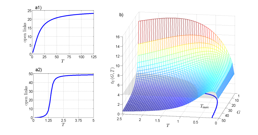
Figure 3: Left two panels: Mean number of open links in equilibrium for Kittel’s molecular zipper as a function of the reservoir temperature $T$ for $N=50$ links, and (a1)) $G=1$ and (a2)) $G=2$. Right panel b): Unfolding time $t_{U}$, Eq. (44), as a function of $T$ and $G$ for $T_{0}=7.5$, $v=0.25$, and $N=2$. Above (below) the horizontal plane in the graph, the opened (closed) state is energetically favored. In the base plane, the temperature $T_{\rm max}$ of maximal unfolding time in dependence of the degeneracy factor $G$ is shown.

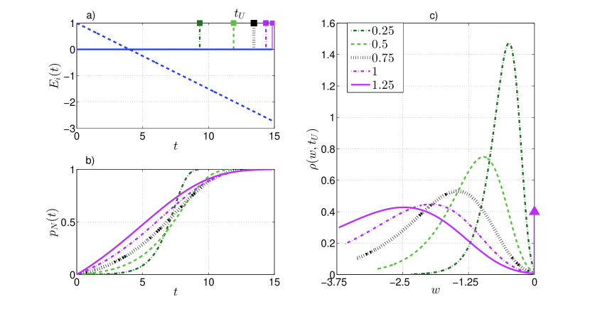
Figure 4: Dynamics of a) the energy levels [Eq. (1)], b) the occupation probability $p_{N}(t)$ of the opened state [Eq. (15)], and c) the probability density $\rho(w,t_{U})$ of the work [Eq. (19)] for $G=1$ and several values of the reservoir temperature $T$. The other parameters are the same as in Fig. 3. The assignment of the line styles to the temperature given in the legend of c) applies also to parts a) and b). In a) we compare the dynamics of the two energy levels with the unfolding time $t_{U}$ [Eq. (44)] at different temperatures marked by the vertical lines. The full (dashed) line gives the energy $E_{1}(t)$ ($E_{2}(t)$) of the closed (unzipped) state. The arrows in c) represent the weights and the positions of the $\delta$-functions, which form the singular part of the probability density.

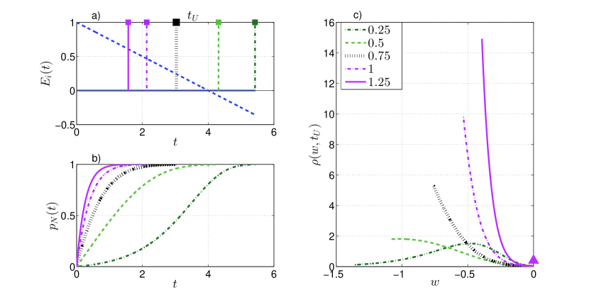
Figure 5: Same quantities as in Fig. 4 for $G=50$ and otherwise the same set of parameters.

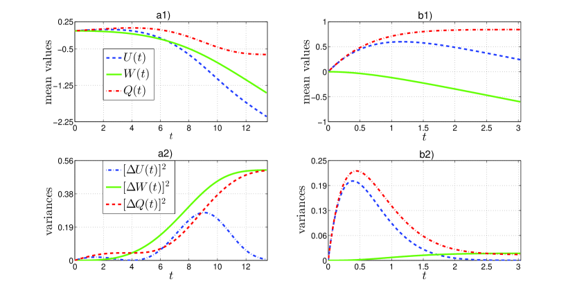
Figure 6: Upper two panels: Mean value of the internal energy [Eq. (20)], work [Eq. (21)] and heat [Eq. (22)] as a function of time for a1) $G=1$ and b1) $G=50$. Lower two panels: Variances of internal energy [Eq. (23)], work [Eq. (24)] and heat [Eq. (25)] as a function of time for a2) $G=1$ and b2) $G=50$. The temperature is $T=0.75$ and the other parameters are the same as in Fig. 3.

For small temperatures [large argument of the exponential and/or small prefactor $g$ in Eq. (4)] the transitions are driven predominantly by the magnitude of the energy gap between the closed and the opened state. For large temperatures [small argument of the exponential and/or large prefactor $g$ in Eq. (4)] by contrast, the dynamics is governed by the entropy difference between the closed and the opened state, and hence by the degeneracy factor $G$. The dependence of the unfolding time $t_{U}$ on $G$ and $T$ is plotted in Fig. 3b) for a representative set of parameters. For any fixed nonzero temperature, the unfolding time decreases with increasing $G$, while for fixed $G$, the temperature-dependence of the unfolding time exhibits a maximum at a temperature $T=T_{{\rm max}}(G)$, where $T_{{\rm max}}(G)$ decreases with increasing $G$, see Fig. 3b).

Let us now consider a certain temperature $T_{0}$ and call, for this temperature, the fast-unzipping regime and slow-unzipping regime the ranges of $G$-values, where $T_{{\rm max}}(G)<T_{0}$ and $T_{{\rm max}}(G)>T_{0}$, respectively. In these two regimes the dynamics and energetics of the molecular zipper exhibit a qualitatively different behavior. In particular we find (i) a different time-dependence of the $N$-th state’s occupation probability, cf. Figs. 4b) and 5b), (ii) a different form of the curves describing the work needed to open the zipper, cf. Figs. 4c) and 5c), (iii) a different mean value of heat accepted by the zipper during the unzipping, cf. Figs. 6a1) and 6b1), and iv) different values of the variances of the internal energy and heat during the unzipping, cf. Figs. 6a2) and 6b2). These features will be now discussed in more detail.

Fig. 4 illustrates the slow-unzipping regime. The probability $p_{N}(t)$ that the zipper has reached the opened state until time $t$ first increases slowly. After the time $d/v$ the energy of the opened state becomes lower than that of the closed one. This leads to more frequent transitions and accordingly $p_{N}(t)$ increases more rapidly. Notice that the curves exhibit a change of their second derivative. The work probability density (WPD) during the unzipping has a maximum located inside its finite support, cf. Fig. 4c). The value of the work at the left (right) border of the support equals the work done on the zipper when it dwells during the time interval $[0,t_{U}]$ in the opened (closed) state. From the position of the WPD peak we can conclude that, for a typical trajectory of the stochastic process $\mathsf{D}(t)$, the work consists of two comparable fractions. The first (second) part of the work is performed while the system dwells in the closed (opened) state. At time $t_{U}$, $0.1\%$ of the trajectories will give molecules still residing in the zipped state. These trajectories contribute to the singular ($\delta$-function) components of WPDs, which are depicted in Fig. 4c) by the vertical arrows [33, 32, 34, 35]. Note that the curves plotted for the temperatures $T=1$ and $T=1.25$, which are close to the temperature $T_{{\rm max}}$(G) for $G=1$, cf. Fig. 3b), become similar to the curves for these temperatures obtained in the fast-unzipping regime for $G=50$, see Fig. 5.

Fig. 5 illustrates the fast-unzipping regime. The probability $p_{N}(t)$ rapidly increases from the very beginning of the process, cf. Fig. 5b), i.e. the zipper opens before the opened state becomes energetically preferred. The maximum of the WPD is located at the left border of its support, cf. Fig. 5c). This means that, for the majority of the trajectories, the substantial part of the work is done while the system dwells in the opened state. Note that the curves plotted for the temperature $T=0.25$, which is close to the boundary temperature $T_{{\rm max}}$(G) for $G=50$, cf. Fig. 3b), become similar to the curves for this temperature in the fast-unzipping regime for $G=1$, see Fig. 4.

Fig. 6 illustrates the dynamics of the thermodynamic quantities (20)–(25) in the two unzipping regimes. For an arbitrary trajectory of $\mathsf{D}(t)$ which resides during the time interval $[t^{\prime},t]$ in the $i$-th state, the work performed on the system is $E_{i}(t)-E_{i}(t^{\prime})$, cf. Eq. (7). In our model, the energies of the states decrease linearly with time and accordingly the mean work is a monotonically decreasing function of time, see Figs. 6a1) and 6b1). Heat is exchanged with the reservoir when the molecule changes its state. It is absorbed by the molecule if the transition brings the molecular zipper to a state with higher energy. Since in our setting the transitions are unidirectional, the molecule necessarily absorbs heat up to the time $t_{E}=d/v$, where the energies of the states become the same, cf. Figs. 4a) and 5a). For times $t>t_{E}$, the molecule delivers heat to the environment. In the slow-unzipping regime we have $t_{U}>t_{E}$. This implies that the mean heat first increases and then decreases, cf. Fig. 6a1). By contrast, in the fast-unzipping regime where $t_{U}<t_{E}$, the mean heat monotonically increases, cf. Fig. 6b1). Finally, due to the transitions to the state with higher energy at the very beginning of the process, cf. Figs. 4 and 5, the mean internal energy (20) develops a single maximum.

The variances of $\mathsf{U}(t)$, $\mathsf{W}(t)$ and $\mathsf{Q}(t)$, cf. Eqs. (23)–(25), are plotted in Figs. 6a2) and Figs. 6b2). If the variance of the internal energy approaches zero, the variance of the work becomes equal to that of the heat. All variances approach constant values at large times. In fact, for $t>t_{U}$, almost all trajectories have brought the molecule into the opened state. As a consequence, the increments to the work, heat and internal energy are nearly constant during the time interval $[t_{U},t]$. Therefore the form of their probability densities does not change, the curves just move along the energy axis.

The probability density for the internal energy has no continuous component. In general it consists of $N$ $\delta$-functions located at the energies of the individual states. The corresponding weights are given by the occupation probabilities of the states. In the slow-unzipping regime, $[\Delta U(t)]^{2}$ vanishes at time $t=0$ and at time $t_{E}=d/v$, when the state energies are equal, and it becomes very close to zero for $t\gtrsim t_{U}$. In between these time instants, the variance develops a maximum, cf. Fig. 6a2). In the fast-unzipping regime, the function $[\Delta U(t)]^{2}$ displays just one maximum, cf. Fig. 6b2), because $t_{U}<t_{E}$.

In both the fast and slow unzipping regime, the variance of the work monotonically increases and approaches a constant for large times, cf. Fig. 6a2) and Fig. 6b2). The absolute value of the first derivate of the variance $[\Delta Q(t)]^{2}$ is given by the product of the two quantities, the energy difference between the closed and the opened states at time $t$ and the probability that the zipper opens at the time $t$, which were shown in Figs. 4 and 5. In the slow-unzipping regime, the majority of the transitions occurs during the time interval $[t_{E},t_{U}]$. During this time interval, the energy difference between the states monotonically increases. In the fast-unzipping regime, by contrast, nearly all transitions take place before time $t_{E}/2$. The sooner the transition, the larger is the amount of transferred heat. As a result, at small times, the heat probability density has one peak at a large value, coming from the trajectories with a transition to the opened state, and another peak at zero heat exchange, originating from trajectories without a transition. With increasing time the amount of the trajectories with a transition to the opened state increases rapidly, and the peak close to zero heat moves towards the peak at a large heat value. This explains the behavior of the heat variances in Figs. 6a2) and 6b2).

Finally, one may ask how our results are affected if the variation (“static disorder”) in base pairing energies is included in the modeling. To this end we have performed Monte Carlo simulations [48] of the stochastic process for a molecular zipper with $N=10$ states, where the initial energies $E_{k}(0)$, $k=1,\ldots,N$, in Eq. (1) are given by $E_{k}(0)=(k-1)(\Delta+\eta_{k})$, corresponding to different losses of energies due to variations in base pair bondings. The $\eta_{k}$ were chosen as random numbers from a box distribution in the interval $[-\Delta/3,\Delta/3]$. Results from these simulations for a number of realizations of this disorder were compared to the predictions of the analytical theory for the ”ordered case”, where $E_{k}(0)=(k-1)\Delta$. We found that, for typical realizations of sets of $\eta_{k}$, the shapes of the work distributions are very similar, while the peak positions and peak heights are shifted slightly. Also the probability distributions $p_{N}(t)$ for the zipper to fully open until time $t$ are, for these sets of $\eta_{k}$, very similar in shape. Analogous to the peak positions of the work distributions, the onset of opening shifts slightly from realization to realization. The shifts of the peaks and of the onset of the opening are controlled by the largest base pair bonding (largest $\eta_{k}$), which governs the unfolding time.

References

References

- [1] Poland D and Scheraga H, 1966 J. Chem. Phys 45 1464
- [2] Hanke A and Metzler R, 2003 J. Phys. A: Math. Gen. 36 L473
- [3] Bicout D J and Kats E, 2004 Phys. Rev. E 70 010902(R)
- [4] Fogedby H C and Metzler R, 2007 Phys. Rev. Lett. 98 070601
- [5] Metzler R, Ambjörnsson T, Hanke A and Fogedby H C, 2009 J. Phys.: Condens. Matter 21 034111
- [6] Gibbs J H and Dimarzio E A, 1959 J. Chem. Phys. 30 271
- [7] Crothers D M, Kallenbach N R and Zimm B H, 1965 J. Mol. Biol. 11 802
- [8] Kittel C, 1969 Am. J. Phys. 37 917
- [9] Liphardt D, Onoa B, Smith S, Tinoco I, and Bustamante C, 2001 Science 292 733
- [10] Liphardt D, Dumont S, Smith S, Tinoco I, and Bustamante C, 2002 Science 296 1832
- [11] Lang M J and Block S M, 2003 Am. J. Phys. 71 201
- [12] Onoa B, Dumont S, Liphardt J, Smith S, Tinoco I Jr. and Bustamante C, 2003 Science 299 1892
- [13] Ritort F, 2006 J. Phys.: Condens. Matter 18 R531
- [14] Ritort F, 2008 Adv. Chem. Phys. 137 31
- [15] Tinoco I Jr and Bustamante C, 1999 J. Mol. Biol. 293 271
- [16] Manosas M and Ritort F, 2005 Biophys. J. 88 3224
- [17] Thirumalai D and Hyeon C, 2005 Biochemistry 44 4957
- [18] Finkelstein A V, 2004 Proteins: structural, thermodynamic and kinetic aspects. In J. L. Barrat and J. Kurchan, editors, Slow relaxations and nonequilibrium dynamics (Berlin: Springer-Verlag)
- [19] R. Green, and H. F. Noller 1997, Annu. Rev. Biochem. 66 679
- [20] Ramakrishnan V, 2002 Cell 108 557
- [21] Kornberg A and Baker T A, 1992 DNA Replication (New York: W. H. Freeman and Company)
- [22] Tackett A J, Morris P D, Dennis R, Goodwin T E, and Raney K D, 2001 Biochemistry 40 543
- [23] Palassini M and Ritort F, 2011, Phys. Rev. Lett. 107 060601
- [24] Esposito M, Van den Broeck C, 2010 Phys. Rev. Lett., 104 (2010) 090601; ibid., Phys. Rev. E 82 011143
- [25] Van den Broeck C, Esposito M, 2010 Phys. Rev. E 82 011144
- [26] Seifert U, 2008 Eur. Phys. J. B 64 423
- [27] Braun O, Hanke A, and Seifert U, 2004 Phys. Rev. Lett. 93 158105
- [28] Crooks G E, 1999 Phys. Rev. E 60 2721
- [29] Jarzynski C, 1997, Phys. Rev. Lett. 78, 2690.
- [30] Chatelain C and Karevski D, 2006 J. Stat. Mech. P06005
- [31] Híjar H, Quintana J and Sutmann G, 2007 J. Stat. Mech. P04010
- [32] Chvosta P, Reineker P and Schulz M, 2007 Phys. Rev. E 75 041124
- [33] Subrt E and Chvosta P, 2007 J. Stat. Mech., P09019.
- [34] Einax M and Maass P, 2009 Phys. Rev. E 80 020102
- [35] Chvosta P, Einax M, Holubec V, Ryabov A and Maass P, 2010 J. Stat. Mech. P03002
- [36] Mazonka O and Jarzynski C, 1999 arXiv:cond-mat/9912121v1
- [37] Baule A and Cohen E D G, 2009 Phys. Rev. E 80 011110
- [38] Manosas M, Mossa A, Forns N, Huguet J M and Ritort F, 2009 J. Stat. Mech. P02061
- [39] Lubensky D K and Nelson D R, 2000 Phys. Rev. Lett. 85 1572
- [40] Engel S, Alemany A, Forns N, Maass P and Ritort F, 2011 Phil. Mag. B 91 2049
- [41] Mossa A, Manosas M, Forns N, Huguet J M and Ritort F, 2009 J. Stat. Mech. P02060
- [42] Bell I G, 1978 Science 200 618
- [43] Smaller (larger) would correspond to saddle points lying closer to state () in configuration space. The derivations in Secs. 3 and 4 can be performed analogously for any and .
- [44] Cocco S, Monasson R and Marko J F, 2001 Proc. Nat. Acad. Sci. 98 8608
- [45] Alemany A, Ribezzi M and Ritort F, 2011 AIP Conference Proceedings 1332 96
- [46] Force controlled experiments are achievable with magnetic tweezers or with optical tweezers operating in the force clamp mode. In the latter case, the conjugate variable to the applied force should better be taken as the trap-pipette distance (rather than the molecular extension) because for this definition the fluctuation theorems are obeyed. Both definitions differ only by a boundary term involving the final and initial forces and , respectively (for details, see [45]).
- [47] In this case one can show that , where from Eq. (1) and , , is the free energy for an equilibrated system with state energies (protocol variables) at time ; is the probability for the zipper to be in the fully closed state under the reversed protocol, if the states are initially distributed according to the equilibrium distribution .
- [48] Holubec V, Chvosta P, Einax M and Maass P, 2011 Europhys. Lett. 93 40003
- [49] Imparato A and Peliti L, 2005 Europhys. Lett. 69 643
- [50] Imparato A and Peliti L, 2005 Europhys. Lett. 70 740