From light to mass: accessing the initial and present-day Galactic globular cluster mass functions

Abstract

The initial and present-day mass functions (ICMF and PDMF, respectively) of the Galactic globular clusters (GCs) are constructed based on their observed luminosities, the stellar evolution and dynamical mass-loss processes, and the mass-to-light ratio (MLR). Under these conditions, a Schechter-like ICMF is evolved for approximately a Hubble time and converted into the luminosity function (LF), which requires finding the values of 5 free parameters: the mean GC age ($\overline{t}_{gc}$), the dissolution timescale of a $10^{5}\,\mbox{$\rm M_{\odot}$}$ cluster ($\tau_{5}$), the exponential truncation mass ($\mathcal{M}_{c}$) and 2 MLR parametrising constants. This is achieved by minimising the residuals between the evolved and observed LFs, with the minimum residuals and realistic parameters obtained with MLRs that increase with luminosity (or mass). The optimum PMDFs indicate a total stellar mass of $\sim 4\times 10^{7}$ $\rm M_{\odot}$ still bound to GCs, representing $\sim 15\%$ of the mass in clusters at the beginning of the gas-free evolution. The corresponding ICMFs resemble the scale-free MFs of young clusters and molecular clouds observed in the local Universe, while the PDMFs follow closely a lognormal distribution with a turnover at $\mbox{$\mathcal{M}_{to}$}\sim 7\times 10^{4}$ $\rm M_{\odot}$. For most of the GC mass range, we find an MLR lower than usually adopted, which explains the somewhat low $\mathcal{M}_{to}$. Our results confirm that the MLR increases with cluster mass (or luminosity), and suggest that GCs and young clusters share a common origin in terms of physical processes related to formation.

1 Introduction

Globular clusters (GCs) are the living fossils of an epoch dating back to the time of Milky Way’s formation and thus, they probably share the same physical conditions and processes that originated our Galaxy. Since formation, GCs are continuously affected by several sources of mass loss but, because of a large initial mass and/or an orbit that takes them most of the time away from the Galactic centre and/or disk, they are, in general, characterised by a long longevity. This suggests that some primordial information may have been preserved, if not at the individual scale, at least with respect to the collective properties shared by the surviving GC population.

In this context, an interesting issue is the origin of the Milky Way’s (old) GC population and its relation to the young massive clusters that form in starbursts and galaxy mergers of the local Universe. If both old and young cluster populations share a similar, starburst origin, the mass distribution of their members should also be characterised by similar mass functions (MFs), something that is ruled out by observations in several local galaxies. For instance, when expressed in terms of the number of GCs per unit logarithmic mass-interval ($dN/d\log\mathcal{M}$), the MFs of young clusters in several galaxies follow monotonically a power law of slope $\approx-1$, while the present-day GC MF (PDMF) presents a turnover for masses lower than $\mbox{$\mathcal{M}_{to}$}\sim 10^{5}\,\mbox{$\rm M_{\odot}$}$ (McLaughlin & Fall 2008 and references therein). The low-mass drop in the lognormal PDMF has been interpreted as mainly due to the large-scale dissolution of low-mass GCs after several Gyrs of tidal interactions with the Galaxy and internal dynamical processes (e.g. McLaughlin & Fall 2008; Kruijssen 2008; Kruijssen & Portegies Zwart 2009).

Consequently, since mass loss continuously changes the MF shape - especially in the low-mass range, a direct comparison of the several Gyr-old PDMF with the MF of young clusters should not be used to draw conclusions on a physical relation between both populations. On the other hand, this raises another, but related question of whether or not the initial MFs (ICMFs) of globular and young clusters are similar, since theoretical evidence suggest that cluster formation leaves distinct imprints in the ICMFs (Elmegreen & Falgarone 1996). Thus, if both cluster populations have the same origin, this should be reflected in the respective ICMFs.

Given the above, the reconstruction of Milky Way’s GC ICMF requires having access not only to the (as complete as possible) PDMF, but also to the mass-loss physics. As for the latter, recent numerical simulations and semi-analytical models have produced robust relations for the mass evolution of star clusters located in different environments and losing mass through stellar evolution and tidal interactions with Galactic substructures and giant molecular clouds (e.g. Lamers et al. 2005; Lamers, Baumgardt & Gieles 2010).

Over the years, the GCMF time evolution has been investigated with a wide variety of approaches. For instance, Vesperini (1998) takes the effects of stellar evolution, two-body relaxation, disc shocking, dynamical friction, and the location in the Galaxy into account to follow the evolution of individual GCs. The main findings are: the large-scale disruption of GCs in the central parts of the Galaxy leads to a flattening in their spatial distribution; if the initial GCMF shape is lognormal, it is preserved in most cases; and in the case of an initial power-law GCMF, evolutionary processes tend to change it into lognormal. Baumgardt (1998) considers GC systems formed with a power-law MF and follows the orbits of individual clusters. Taking several GC destruction mechanisms into account, he finds luminosity distributions that depend on Galactocentric distance. Vesperini et al. (2003) study the dynamical evolution of M 87 GCs with numerical simulations that cover a range of initial conditions for the GCMF and for the spatial and velocity distribution of the GCs. The simulations include the effects of two-body relaxation, dynamical friction, and stellar evolution-related mass loss. They confirm that an initial power-law GCMF can be changed into bell-shaped through dynamical processes, and show that the inner flattening observed in the spatial distribution of M 87 GCs can result from the dynamical evolution on an initially steep density profile. Parmentier & Gilmore (2007) show that an approximately Gaussian MF is naturally generated from a power-law mass distribution (but with a lower-mass limit) of protoglobular clouds by expulsion from the protocluster of star-forming gas due to supernova activity. Shin, Kim & Takahashi (2008) targets the MF and radial distribution evolution of the Galactic GCs by means of a Fokker-Planck model that considers dynamical friction, disc/bulge shocking and eccentric GC orbits. Their best-fit models predict the initial GC mass as $M_{GC}^{0}\sim(1.5-1.8)\times 10^{8}\,\mbox{$\rm M_{\odot}$}$.

At some point, most of the previous works compare models with the observed GC PDMF. However, especially because of the large distances involved, a direct determination of the stellar mass for most GCs is not available, which means that the observational PDMF cannot be taken as an ideal starting point for this analysis. Instead, the most direct and robust observable available for the present-day Milky Way’s GC population as a whole is the luminosity function (LF), which is usually expressed in terms of the absolute $V$ magnitude. Obviously, the use of luminosity requires a mass-to-light relation (MLR) to convert LFs into MFs.

Recent observational and theoretical findings have convincingly shown that the MLR is not constant with respect to cluster mass. Instead, the dynamical evolution of clusters - and the preferential loss of low-mass stars - also affects the MLR. Specifically, for a given age and metallicity, the MLR is expected to increase with cluster mass (or luminosity; e.g. Kruijssen 2008; Kruijssen & Portegies Zwart 2009). Interestingly, the MLR dependence on luminosity (or mass) is already suggested by the dynamical cluster mass and MLR estimates of Pryor & Meylan (1993).

Our goal with the present paper is to reconstruct both the ICMF and PDMF of the Galactic GCs, starting with their observed LF and taking the mass loss into account. In this process, different analytical forms of the MLR will be tested to search for constraints.

The present paper is organised as follows. In Sect. 2 we build the observed and theoretical LFs of the Galactic GCs, convert the latter into the PDMF, and discuss the adopted MLRs. In Sect. 3 we briefly describe the parameter-search method. In Sect. 4 we discuss the results. Concluding remarks are given in Sect. 5.

2 The theoretical present-day LF

The first step in our analysis is to build the observed (or present-day) LF ($\phi(M_{V})\equiv\,d\,N/d\,M_{V}$, i.e., number of GCs per unit absolute magnitude interval) of the Galactic GCs. The data were taken from the 2010 revision of the catalogue compiled by Harris (1996), which contains 156 GCs with bona-fide absolute magnitudes in the V band ($M_{V}$). By definition, the integral of $\phi(M_{V})$, over the full $M_{V}$ range is the input number of GCs. As a caveat, we note that several works indicate that not all Galactic GCs share a common history (e.g. Bica et al. 2006 and references therein), with some having been accreted from dwarf galaxies (e.g. Hilker & Richtler 2000; Parmentier et al. 2000) and others associated with the Galactic thick disc (e.g. Zinn 1985).

Following previous work (e.g. Bonatto & Bica 2011), uncertainties in $M_{V}$ are incorporated in the LF by assuming a normal (Gaussian) distribution of errors. Specifically, if the magnitude and standard deviation of a GC (usually, the mean value over a series of independent measurements) are given by $\bar{M}_{V}\pm\sigma$, the probability of finding it at a specific value $M_{V}$ is given by $P(\mbox{$M_{V}$})=\frac{1}{\sqrt{2\pi}\sigma}\,e^{{-\frac{1}{2}}\left(\frac{M_{V}-\bar{M}_{V}}{\sigma}\right)^{2}}$. Next, we build a grid of bins covering the full $M_{V}$ range in Harris (1996) and, for each bin, we sum the $M_{V}$ density (or probability) for all GCs (i.e., the difference of the error function computed at the bin borders). However, since uncertainties are not given in Harris (1996), for simplicity we adopt relative errors that depend on the apparent magnitude ($m_{V}$) as $\epsilon=0.1\,e^{(m_{V}/27)}$. Thus, relatively bright ($m_{V}\la 10$) GCs have $\epsilon\la 0.15$, while fainter ones ($m_{V}\ga 20$) have $\epsilon\ga 0.2$. Finally, we assume that the absolute error in $M_{V}$ is simply given by $\sigma=\epsilon\times\left|M_{V}\right|$. As shown in Bonatto & Bica (2011), the end result is a distribution function significantly smoother than a classical histogram. Indeed, the observed LF (Fig. 1) is approximately gaussian-shaped with a pronounced peak around $M_{V}\approx-7$ and $\approx 4$ mags of full width at half maximum.

As usual with respect to distribution functions, the observed $\phi(M_{V})$ can be linked to the PDMF, $\xi(\mbox{$\mathcal{M}$})\equiv\,d\,N/d\,\mbox{$\mathcal{M}$}$, by

$$\phi(M_{V})=\xi(\mbox{$\mathcal{M}$})\left|\frac{d\,\mbox{$\mathcal{M}$}}{d\,M_{V}}\right|.$$ (1)

However, except for a few cases, the stellar mass of most GCs has not been directly measured, and so, the actual shape of $\xi(\mbox{$\mathcal{M}$})$ remains uncertain. On the other hand, $\xi(\mbox{$\mathcal{M}$})$ can be inferred if one knows the initial MF, the GCs age, and the mass-loss physics. Formally, if $\xi_{o}(\mbox{$\mathcal{M}$}_{o})$ is the MF at $t_{o}$ - and assuming that GCs are not formed subsequently, the MF at a later time $t$ is given by

$$\xi(\mbox{$\mathcal{M}$},t)=\xi_{o}(\mbox{$\mathcal{M}$}_{o})\left|\frac{\partial\mbox{$\mathcal{M}$}_{o}}{\partial\mbox{$\mathcal{M}$}}\right|,$$ (2)

where $\mbox{$\mathcal{M}$}=\mbox{$\mathcal{M}$}(\mbox{$\mathcal{M}$}_{o},t)$, and $\mbox{$\mathcal{M}$}_{o}$ represents the individual GC masses at $t_{o}$.

Several works (e.g. Portegies Zwart, McMillan & Gieles 2010; Larsen 2009) suggest that star clusters form with a mass distribution that follows the truncated power-law of Schechter (1976)

$$\xi_{o}(\mbox{$\mathcal{M}$}_{o})=\mbox{$k_{s}$}\mbox{$\mathcal{M}$}_{o}^{-2}e^{-\left(\mbox{$\mathcal{M}$}_{o}/\mbox{$\mathcal{M}$}_{c}\right)}$$ (3)

over the mass range $[\mbox{$\mathcal{M}$}_{inf}$ – $\mbox{$\mathcal{M}$}_{sup}]$, where $\mbox{$\mathcal{M}$}_{c}$ is the exponential truncation mass, and $k_{s}$ is a normalisation constant. We note that, because of the continuous mass loss (see below), GCs that formed with a relatively low mass may no longer be detected, and can be considered as dissolved. Here, we represent this dissolution limit by the lower observable mass value $\mbox{$\mathcal{M}$}_{i}$.

The earliest cluster phase is dominated by effects related to the impulsive removal of the parental, intra-cluster gas by supernovae and massive-star winds, which rapidly damps cluster formation and changes the ratio between residual gravitational potential and stellar velocity dispersion, thus leading to the first bout of dynamical evolution (e.g. Lada, Margulis & Dearborn 1984; Goodwin 1997; Geyer & Burkert 2001; Baumgardt & Kroupa 2007). Another consequence of these early effects on the ICMF may be a depletion in the number of GCs towards the low-mass range (e.g. Kroupa & Boily 2002; Baumgardt, Kroupa & Parmentier 2008; Parmentier et al. 2008). Clusters can be considered to be essentially gas free after the first $\mbox{$t_{o}$}\sim 10^{7}$ yrs, but they keep losing mass mainly through stellar evolution and externally-driven tidal effects. After several Gyrs, these processes may reduce the mass to a fraction of the initial value. Following Lamers et al. (2005), we express the mass remaining (due to stellar evolution and tidal effects) in a given GC (with initial mass $\mbox{$\mathcal{M}$}_{o}$) at time $t$ by

$$\mbox{$\mathcal{M}$}(t)=\mbox{$\mathcal{M}$}_{o}\left[\mu_{se}^{\gamma}-\frac{\gamma\,t}{\tau_{5}}\left(\frac{\mbox{$\mathcal{M}$}_{o}}{10^{5}\mbox{$\rm M_{\odot}$}}\right)^{-\gamma}\right]^{1/\gamma},$$ (4)

where $\mu_{se}$ is the stellar evolution mass loss, $\tau_{5}$ is the dissolution timescale of a $10^{5}\,\mbox{$\rm M_{\odot}$}$ star cluster, and $\gamma$ is the power-law exponent that sets the dependence of the cluster disruption time on mass. We note that $\mu_{se}$ is a function of time, but since we are dealing with GCs with ages between 9-13 Gyr, we simplify this point by taking here the asymptotic value $\mu_{se}\approx 0.7$ (Lamers et al. 2005). Useful Milky Way approximations for the other parameters are $\gamma\approx 0.7$ (Lamers, Baumgardt & Gieles 2010), and $\tau_{5}\approx 10^{4}$ Myr (Kruijssen & Cooper 2011 and references therein). However, $\tau_{5}$ is expected to present a significant dispersion around its quoted value to account for different GC environments and orbital conditions (Kruijssen & Cooper 2011). In this sense, we consider $\tau_{5}$ to be a free parameter allowed to vary within a given range (Sect. 3). Thus, inverting Eq. 4 to have $\mbox{$\mathcal{M}$}_{o}=\mbox{$\mathcal{M}$}_{o}(\mbox{$\mathcal{M}$}(t))$ and coupling Eqs. 2 and 3, the PDMF can be expressed as

$$\xi(\mbox{$\mathcal{M}$},t)=\mbox{$k_{s}$}\mu_{se}\mbox{$\mathcal{M}$}^{\gamma-1}\left(\mbox{$\mathcal{M}$}^{\gamma}+\beta\,t\right)^{-(1+1/\gamma)}e^{-\frac{\left(\mathcal{M}^{\gamma}+\beta\,t\right)^{1/\gamma}}{\mu_{se}\mathcal{M}_{c}}},$$ (5)

where $\beta\equiv(\gamma 10^{5\gamma})/\tau_{5}$.

Formally, Eq. 5 applies to an individual cluster having evolved over a time $t$ after $t_{o}$. However, the underlying idea of our approach is to consider not the individual, but the collective - or average - evolution of the full sample of the Galactic GCs until now. This adds another component to our approach because, instead of a single formation event, the Milky Way GCs present some dispersion in age (e.g. Marín-Franch et al. 2009). In this sense, $t$ should be taken as the mean - or at least, the representative - age ($\overline{t}_{gc}$) of the GC population. So, hereafter we consider $t=\mbox{$\overline{t}_{gc}$}$. The constant $k_{s}$ can be computed by noting that the integral of Eq. 5 over the minimum observable GC mass, $\mbox{$\mathcal{M}$}_{i}$, and the maximum remaining mass at time $\overline{t}_{gc}$, $\mbox{$\mathcal{M}$}_{s}=\mbox{$\mathcal{M}$}_{sup}(\mbox{$\overline{t}_{gc}$})$, corresponds to the present-day number of GCs ($N_{GC}$)

$$N_{GC}=\int_{\mathcal{M}_{i}}^{\mathcal{M}_{s}}\xi(\mbox{$\mathcal{M}$},\mbox{$\overline{t}_{gc}$})\,d\,\mbox{$\mathcal{M}$}.$$ (6)

Changing variables in the integral, Eq. 6 can be reduced to

$$N_{GC}=\frac{\mbox{$k_{s}$}}{\mbox{$\mathcal{M}$}_{c}}\int_{\tau_{i}}^{\tau_{s}}\left[\tau\ln(\tau)\right]^{-2}d\,\tau=\frac{\mbox{$k_{s}$}}{\mbox{$\mathcal{M}$}_{c}}\left[E1\,(\ln(\tau))-\frac{1}{\tau\ln(\tau)}\right]_{\tau_{i}}^{\tau_{s}},$$

where $E1$ is the exponential integral,

$$\ln(\tau_{i})=\left(\mbox{$\mathcal{M}$}_{i}^{\gamma}+\beta\,\mbox{$\overline{t}_{gc}$}\right)^{1/\gamma}/\left(\mu_{se}\mathcal{M}_{c}\right),$$

and

$$\ln(\tau_{s})=\left(\mbox{$\mathcal{M}$}_{s}^{\gamma}+\beta\,\mbox{$\overline{t}_{gc}$}\right)^{1/\gamma}/\left(\mu_{se}\mathcal{M}_{c}\right).$$

Summarising, the predicted PDMF (Eq. 5) can be inserted into Eq. 1 to build the theoretical LF $\widetilde{\phi}(M_{V})$ and, with the usual relation between luminosity ($L_{V}$) and absolute magnitude $L_{V}=10^{-0.4(M_{V}-M_{V}^{\odot})}$, with $M_{V}^{\odot}=4.83$, the theoretical LF is expressed as

$$\widetilde{\phi}(M_{V})=0.4\,\xi(\mbox{$\mathcal{M}$},\mbox{$\overline{t}_{gc}$})\,\frac{d\,\mbox{$\mathcal{M}$}}{d\,\log{L_{V}}}.$$ (7)

Subsequently, $\widetilde{\phi}(M_{V})$ can be compared with the observed $\phi(M_{V})$ to search for the parameters that lead to the best match between both. Note that the present-day GC masses in Eq. 7 should be expressed as a function of $M_{V}$ (through $L_{V}$), which can be done by means of a mass-to-light relation ($MLR\equiv\mbox{$\mathcal{M}$}/L_{V}$).

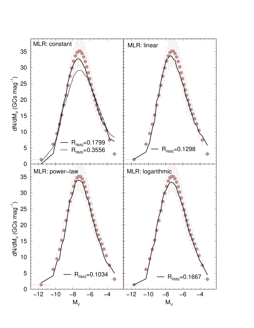
Figure 1: The observed (light-shaded symbols) and best-fit LFs (solid line) produced with alternative MLRs. The respective $R_{rms}$ are shown. A constant MLR with the mean value of $\mbox{$\mathcal{M}$}/L_{V}=2$ (dotted line) taken from the literature produces a relatively poor fit with $\mbox{$R_{rms}$}\approx 0.36$ (top-left panel).

2.1 The mass-to-light ratio

According to Sect. 1 and Eq. 7, it is clear that the dependence of MLR on luminosity (or mass) is central to the task of building MFs from the observed LF. In this sense, we consider here the following comprehensive range of MLR shapes, (i) constant: $\mbox{$\mathcal{M}$}/L_{V}=a$; (ii) linearly-increasing with luminosity: $\mbox{$\mathcal{M}$}/L_{V}=a+b\,L_{V}$; (iii) power-law: $\mbox{$\mathcal{M}$}/L_{V}=a+b\,L_{V}^{n}$; and (iv) logarithmic: $\mbox{$\mathcal{M}$}/L_{V}=a+b\,\log(L_{V})$, where $a$ and $b$ are constants. Note that for practical reasons (i.e., the need of an analytical expression to convert $M_{V}$ into $\mathcal{M}$ in Eq. 7), we express the MLR as a function of $L_{V}$ and not mass.

Obviously, once the MLR constants $a$ and $b$ have been assigned values, the minimum and maximum present-day GC masses ($\mbox{$\mathcal{M}$}_{i}$ and $\mbox{$\mathcal{M}$}_{s}$) are naturally determined from the respective faint and bright boundaries of the observed LF. And, for a given mean GC age ($\overline{t}_{gc}$), a similar reasoning leads to the maximum GC mass ($\mbox{$\mathcal{M}$}_{sup}$) at $t_{o}$ through inversion of Eq. 4.

3 Searching for the optimum parameters

The approach summarised by Eq. 7 contains some poorly-known (and unknown) parameters, such as the mean cluster age ($\overline{t}_{gc}$), the dissolution timescale ($t_{5}$), the truncation mass ($\mbox{$\mathcal{M}$}_{c}$), and the MLR constants $a$ and $b$. Our approach considers these five parameters as free. However, we note that some dependence among these parameters should be expected to occur, especially for very wide search ranges. For instance, a short $\overline{t}_{gc}$ would result in a low $\tau_{5}$ to hasten dissolution over a shorter age range. Similarly, a lower MLR would shift the MF turnover to a lower cluster mass, which could result from a longer dissolution timescale (i.e. less dynamical evolution) for a given mean cluster age. We minimise this effect by adopting a reasonable GC age range (see below).

Thus, the task now is to search for values for the set of free parameters $\mbox{$\vec{P}$}\equiv\left\{a,b,\mbox{$\overline{t}_{gc}$},t_{5},\mbox{$\mathcal{M}$}_{c}\right\}$ that produces the best match between the observed and theoretical LFs, $\phi(M_{V})$ and $\tilde{\phi}(M_{V})$, respectively. This is achieved by minimising the root mean squared residual ($R_{rms}$) between both functions. By construction, $R_{rms}$ is a function of the free parameters, i.e., $\mbox{$R_{rms}$}=\mbox{$R_{rms}$}(\mbox{$\vec{P}$})$, which we express as

$$\mbox{$R_{rms}$}=\sqrt{\frac{1}{N_{GC}}\sum_{j=1}^{n_{b}}\frac{\left[\tilde{\phi}(M^{j}_{V})-\phi(M^{j}_{V})\right]^{2}}{\tilde{\phi}(M^{j}_{V})+\phi(M^{j}_{V})}},$$ (8)

where the sum occurs over the $n_{b}$ non-zero magnitude bins of the observed LF. The normalisation by the theoretical$+$observed density of GCs in each bin gives a higher weight to the more populated bins. Finally, the squared sum is divided by the total number of observed GCs, which makes $R_{rms}$ dimensionless and preserves the number statistics when comparing LFs built with unequal GC populations.

Table 1: Present-day and initial MF parameters found with alternative MLRs

Free Parameters

Derived Parameters

Rank

$R_{rms}$

$\overline{t}_{gc}$

$a$

$b$

$\mbox{$\mathcal{M}$}_{c}$

$\tau_{5}$

$\mbox{$\mathcal{M}$}_{i}$

$\mbox{$\mathcal{M}$}_{sup}$

$N_{GC}^{0}$

$M_{GC}^{0}$

$M_{GC}^{now}$

(Gyr)

($\rm M_{\odot}$)

(Gyr)

($10^{3}\,\mbox{$\rm M_{\odot}$}$)

$(10^{7}\,\mbox{$\rm M_{\odot}$})$

($10^{4}$)

($10^{8}\,\mbox{$\rm M_{\odot}$}$)

($10^{6}\,\mbox{$\rm M_{\odot}$}$)

(1)

(2)

(3)

(4)

(5)

(6)

(7)

(8)

(9)

(10)

(11)

(12)

Constant: $\mbox{$\mathcal{M}$}/L_{V}=a$

$(\times 10^{5})$

Abs.Min.

0.1799

10.7

0.59

—

6.0

5.8

0.7

0.5

9.9

4.4

9.2

$\rm\overline{1\%~{}Low.}$

0.1875

$11.4\pm 1.0$

$0.49\pm 0.19$

—

$5.1\pm 2.0$

$8.1\pm 4.3$

$0.7\pm 0.3$

$0.4\pm 0.2$

$8.4\pm 1.7$

$3.7\pm 1.4$

$8.3\pm 3.2$

$\rm\overline{Overall}$

0.2041

$11.3\pm 1.0$

$0.50\pm 0.23$

—

$5.5\pm 2.7$

$8.7\pm 5.3$

$0.8\pm 0.4$

$0.4\pm 0.3$

$7.5\pm 2.0$

$3.4\pm 1.5$

$8.4\pm 3.9$

Logarithmic: $\mbox{$\mathcal{M}$}/L_{V}=a+b\,\log(L_{V})$

$(\times 10^{-1})$

$(\times 10^{6})$

Abs.Min.

0.1667

10.3

0.32

0.19

1.6

5.0

0.7

1.2

7.3

3.8

17

$\rm\overline{1\%~{}Low.}$

0.1772

$11.1\pm 1.1$

$0.19\pm 0.21$

$0.15\pm 0.05$

$1.3\pm 0.5$

$7.8\pm 4.5$

$0.8\pm 0.3$

$0.7\pm 0.4$

$5.8\pm 1.2$

$2.9\pm 1.0$

$14\pm 5$

$\rm\overline{Overall}$

0.1936

$11.4\pm 1.0$

$0.65\pm 0.66$

$0.16\pm 0.05$

$1.5\pm 0.6$

$6.9\pm 2.7$

$0.9\pm 0.3$

$0.8\pm 0.5$

$5.3\pm 1.1$

$3.1\pm 1.0$

$16\pm 5$

Linear: $\mbox{$\mathcal{M}$}/L_{V}=a+b\,L_{V}$

$(\times 10^{-5})$

$(\times 10^{10})$

Abs.Min.

0.1298

12.6

0.43

0.20

1.6

5.4

0.6

26

1.9

1.2

21

$\rm\overline{1\%~{}Low.}$

0.1345

$11.4\pm 1.1$

$0.91\pm 0.47$

$0.45\pm 0.23$

$5.2\pm 2.8$

$9.7\pm 6.1$

$1.4\pm 0.8$

$13\pm 15$

$1.7\pm 0.6$

$2.7\pm 1.4$

$41\pm 22$

$\rm\overline{Overall}$

0.1543

$11.3\pm 1.1$

$0.93\pm 0.44$

$0.46\pm 0.22$

$5.0\pm 2.8$

$9.1\pm 5.7$

$1.5\pm 0.8$

$18\pm 22$

$1.7\pm 0.3$

$1.7\pm 1.3$

$42\pm 20$

Power-law: $\mbox{$\mathcal{M}$}/L_{V}=a+b\,L_{V}^{0.67}$

$(\times 10^{-3})$

$(\times 10^{10})$

Abs.Min.

0.1034

10.5

0.83

0.36

1.6

5.8

1.8

5.3

1.7

3.1

44

$\rm\overline{1\%~{}Low.}$

0.1213

$11.3\pm 0.9$

$0.72\pm 0.33$

$0.29\pm 0.14$

$5.1\pm 2.8$

$8.8\pm 4.8$

$1.2\pm 0.6$

$7.0\pm 6.7$

$2.2\pm 0.4$

$2.7\pm 1.3$

$37\pm 17$

$\rm\overline{Overall}$

0.1395

$11.3\pm 0.8$

$0.71\pm 0.34$

$0.28\pm 0.13$

$5.0\pm 2.8$

$9.0\pm 5.5$

$1.2\pm 0.6$

$6.8\pm 6.8$

$2.1\pm 0.4$

$2.6\pm 1.2$

$36\pm 17$

• Cols. (1) and (2): Rank and corresponding $R_{rms}$ value; Col. (3): mean GC age; Cols. (4) and (5): MLR constants; Col. (6) exponential truncation mass; Col. (7): dissolution timescale of a $10^{5}\,\mbox{$\rm M_{\odot}$}$ star cluster; Col. (8): lowest present-day (observed) GC mass; Col. (9): upper cluster mass at $t_{o}$; Cols. (10) and (11): number and total mass of GCs at $t_{o}$ (with $\mbox{$\mathcal{M}$}_{inf}\ga 10^{2}\,\mbox{$\rm M_{\odot}$}$); Col. (12): present-day total GC mass.

Among the several minimisation methods available in the literature, the adaptive simulated annealing (ASA) is adequate to our purposes, because it is relatively time efficient, robust and capable to distinguish between different local minima (e.g. Goffe, Ferrier & Rogers 1994). The first step in the minimisation process is to define individual search ranges (and variation steps) for each free parameter. Next, initial values are randomly selected for all free parameters (i.e., the initial point $\vec{P}_{o}$ in the $R_{rms}$ hyper-surface) and the starting value of $R_{rms}$ is computed. Then ASA takes a step by changing the initial parameters ($\mbox{$\vec{P}_{o}$}\rightarrow\mbox{$\vec{P}$}$), and a new value of $R_{rms}$ is evaluated. Specifically, this implies that a new LF is built with the changed parameters. By definition, any step that decreases $R_{rms}$ (downhill) is accepted, with the process repeating from this new point. However, uphill steps may also be taken, with the decision made by the Metropolis (Metropolis et al. 1953) criterion, which has the advantage of enabling ASA to escape from local minima. The variation steps become smaller as the minimisation is successful and ASA approaches the global minimum ($\mbox{$\vec{P}$}\rightarrow\mbox{$\vec{P}_{min}$}$).

The output of a single ASA run is the set of optimum values $\vec{P}_{min}$ (expected to correspond to the global minimum) and the respective $R_{rms}$, but with no reference to uncertainties. However, given the errors associated to the observed LF (Fig. 1), uncertainties to the derived parameters are strongly required. Thus, we run ASA several times ($N_{run}$) allowing for different starting points ($\vec{P}_{o}$) and taking the uncertainty of each $M_{V}$ bin in the observed LF (Fig. 1) into account. In the end, we compute the weighted mean of the parameters over a range of runs, using the $R_{rms}$ of each run as weight ($w=1/\mbox{$R_{rms}$}$). As a compromise between statistical significance and computational time, we adopt here $\mbox{$N_{run}$}=6000$.

The search ranges adopted here try to emulate the physical conditions prevailing in the Milky Way. In this sense, the mean GC age runs through $9\leq\mbox{$\overline{t}_{gc}$}(Gyr)\leq 13$; the exponential truncation mass within $10^{4}\leq\mbox{$\mathcal{M}$}_{c}(\mbox{$\rm M_{\odot}$})\leq 10^{11}$; and the dissolution timescale within $5\leq\tau_{5}(Gyr)\leq 30$ (to account for different environments and orbital conditions). Initially, the MLR constants $a$ and $b$ were allowed to vary within $0$ and $10$ but, after a few runs, their ranges were fine-tuned to more constrained ranges.

4 Results and discussion

The approach described in Sect. 3 was applied to the four MLR modes discussed in Sect. 2.1, and the numerical results of the 6000 independent ASA runs are summarised in Table 1. For conciseness, we show only the parameters belonging to the run with the absolute minimum $R_{rms}$, together with those averaged over all the 6000 runs, and those corresponding to the average of 1% of the runs having the lowest $R_{rms}$. The LFs corresponding to the absolute minimum $R_{rms}$ are compared to the observed LF in Fig. 1. Given the relative proximity among the minimum and average parameters (Table 1), the respective LFs of each MLR should also be similar.

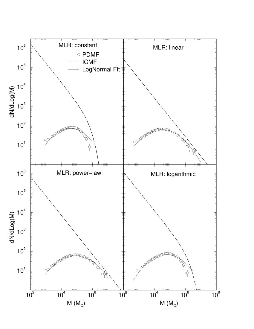
Figure 2: Present-day (empty circles) and initial (dashed-line) MFs that result from different MLRs. The PDMFs (expressed as $d\,N/d\,\log(\mathcal{M})$) are fitted with lognormal curves (thin solid line).

Qualitatively, the adopted MLRs produce similarly evolved LFs (Fig. 1), but with different individual and integrated parameters at the output. As expected, the mean age, in all cases, is consistent with the age of the Galaxy and the age spread of the Galactic GCs (Muratov & Gnedin 2010), ranging within 10 and 12.6 Gyr. Also, the best-fit dissolution timescale falls in the range $5\leq\tau_{5}(Gyr)\leq 10$, a spread that is consistent with the different environments where the Galactic GCs dwell. Below we discuss the results for the MLR modes in a decreasing order of $R_{rms}$.

Before doing so, it is useful to gather some integrated Galactic GC values to be used for comparison with our results. For instance, based on the uniform ratio $\mbox{$\mathcal{M}$}/L_{V}=2$, Mackey & van den Bergh (2005) estimate that the current total mass of halo GCs as $2\times 10^{7}\,\mbox{$\rm M_{\odot}$}$. However, this may be a lower limit to the actual value of $M_{GC}^{now}$, since halo GCs correspond to a sub-population of the Galactic GCs (e.g. Mackey & van den Bergh 2005) and SSP models (e.g. Bruzual & Charlot 2003; Anders & Fritze-von Alvensleben 2003) usually predict the higher ratio $\mbox{$\mathcal{M}$}/L_{V}=2-4$. Also, the initial total mass in GCs ($M_{GC}^{0}$) can be compared with estimates of the current stellar halo mass of $\mathcal{M}_{h}\approx 1\times 10^{9}\,\mbox{$\rm M_{\odot}$}$ (e.g. Freeman & Bland-Hawthorn 2002).

Constant $\left[\mbox{$\mathcal{M}$}/L_{V}=a\right]$: With $\mbox{$R_{rms}$}\sim 0.18-0.2$, the best fit was obtained with $\mbox{$\mathcal{M}$}/L_{V}\approx 0.6$. For such MLR, the lowest present-day GC mass turns out being somewhat low for a GC, $\mbox{$\mathcal{M}$}_{i}\sim 700\,\mbox{$\rm M_{\odot}$}$; the exponential truncation mass is $\mbox{$\mathcal{M}$}_{c}\approx 6\times 10^{5}\,\mbox{$\rm M_{\odot}$}$. Reflecting the low statistical significance of the constant MLR, the dispersion around the mean for most parameters is very large. When combined, the derived parameters imply an exceedingly-low (see above) total mass for the present-day GC population, $M_{GC}^{now}\la 1\times 10^{7}\,\mbox{$\rm M_{\odot}$}$. Assuming 100 $\rm M_{\odot}$ as the lower-limit for cluster formation, the total stellar mass stored in clusters at $t_{o}$ would be $M_{GC}^{0}\sim 4\times 10^{8}\,\mbox{$\rm M_{\odot}$}$. Thus, the fraction of the initial stellar mass still bound in GCs would be as low as $f_{bound}\approx 2\%$. The higher ratio $\mbox{$\mathcal{M}$}/L_{V}=2$ (the average used in previous works, e.g. Kruijssen 2008) leads to an evolved LF that fails to describe the observations, especially around the peak ($M_{V}\approx-7$), with the high value of $\mbox{$R_{rms}$}\sim 0.36$.

Logarithmic $\left[\mbox{$\mathcal{M}$}/L_{V}=a+b\,\log(L_{V})\right]$: With $R_{rms}$ similar to the constant MLR, the logarithmic MLR yields $\mbox{$\mathcal{M}$}_{i}\sim 800\,\mbox{$\rm M_{\odot}$}$, $\mbox{$\mathcal{M}$}_{c}\sim 1.5\times 10^{6}\,\mbox{$\rm M_{\odot}$}$, $M_{GC}^{now}\sim 1.5\times 10^{7}\,\mbox{$\rm M_{\odot}$}$, and $M_{GC}^{0}\sim 3\times 10^{8}\,\mbox{$\rm M_{\odot}$}$, which implies the low bound mass fraction of $f_{bound}\sim 5\%$. These values are similar to those obtained with the constant MLR and, as such, may not be realistic.

Linear $\left[\mbox{$\mathcal{M}$}/L_{V}=a+b\,L_{V}\right]$: Dropping somewhat to $\mbox{$R_{rms}$}\sim 0.13-0.15$, the linearly increasing MLR predicts the more realistic values of $\mbox{$\mathcal{M}$}_{i}\sim 1.4\times 10^{3}\,\mbox{$\rm M_{\odot}$}$ and $M_{GC}^{now}\sim 4\times 10^{7}\,\mbox{$\rm M_{\odot}$}$. With $M_{GC}^{0}\sim 2\times 10^{8}\,\mbox{$\rm M_{\odot}$}$, the fraction of stellar mass still bound in GCs rises to $f_{bound}\sim 20\%$. Interestingly, the best-fits require an exponential truncation mass of $\mbox{$\mathcal{M}$}_{c}\sim 10^{10}\,\mbox{$\rm M_{\odot}$}$, about 4 orders of magnitude higher than usually adopted (e.g. McLaughlin & Fall 2008).

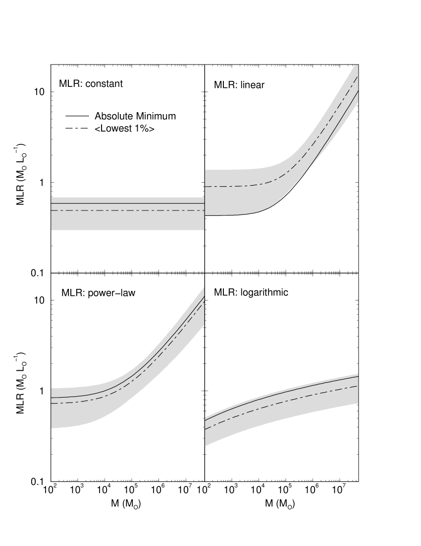
Figure 3: The best-fit MLRs are shown as a function of the cluster mass. For comparison, the curves corresponding to the absolute minimum (solid line) and the 1% runs with the lowest $R_{rms}$ values (dot-dashed) are shown, together with the $1\sigma$ uncertainty domain of the latter.

Power-law $\left[\mbox{$\mathcal{M}$}/L_{V}=a+b\,L_{V}^{n}\right]$: To minimise the number of free parameters, we applied our approach for several fixed exponents $n$, with the lowest values of $R_{rms}$ ($\sim 0.10-0.14$) obtained with $n=0.67$. The relevant best-fit parameters are $\mbox{$\mathcal{M}$}_{i}\sim 10^{3}\,\mbox{$\rm M_{\odot}$}$, $\mbox{$\mathcal{M}$}_{c}\sim 5\times 10^{10}\,\mbox{$\rm M_{\odot}$}$, $M_{GC}^{now}\sim 4\times 10^{7}\,\mbox{$\rm M_{\odot}$}$, and $M_{GC}^{0}\sim 3\times 10^{8}\,\mbox{$\rm M_{\odot}$}$, with a bound-mass fraction of $f_{bound}\sim 15\%$.

Both the linear and power-law models predict values of $M_{GC}^{now}$ that are compatible with independent estimates. They also imply an initial total GC mass that corresponds to $\la 30\%$ of the current stellar halo mass.

Reflecting the (cluster) mass-dependent nature of the mass-loss processes, GCs having a mass within $(1-2)\times 10^{5}\,\mbox{$\rm M_{\odot}$}$ at the onset of the gas-free phase would have evolved to become the present-day least massive ($\mbox{$\mathcal{M}$}_{i}\sim 1\times 10^{3}\,\mbox{$\rm M_{\odot}$}$) GCs. This means that, after a Hubble time of evolution in the Galaxy, GCs occupying the low-mass tail of the PDMF retain only $\sim 1\%$ of their initial stellar mass. Regarding the total stellar mass still bound in GCs, the best-fit MLRs (power-law and linear) imply that $\sim 85\%$ of the mass of the initial GC population would have been lost to the field.

Finally, the best-fit MLRs are shown in Fig. 3 as a function of the cluster mass. Both the constant and logarithmic MLRs are somewhat shallow, with $\mbox{$\mathcal{M}$}/L_{V}\la 2.0$ over the full range of mass ($10^{2}\leq\mbox{$\mathcal{M}$}(\mbox{$\rm M_{\odot}$})\leq 10^{7}$). On the other hand, the linear and power-law MLRs have $\mbox{$\mathcal{M}$}/L_{V}\approx 1.0$ for $10^{2}\leq\mbox{$\mathcal{M}$}(\mbox{$\rm M_{\odot}$})\la 10^{4}$, then rising monotonically for larger masses, reaching $\mbox{$\mathcal{M}$}/L_{V}\approx 2.5$ for $\mbox{$\mathcal{M}$}=10^{6}\,\mbox{$\rm M_{\odot}$}$, and $\mbox{$\mathcal{M}$}/L_{V}\approx 4-8$ for $\mbox{$\mathcal{M}$}=10^{7}\,\mbox{$\rm M_{\odot}$}$. When converted to a function of GC mass, the power-law MLR follows the relation

$$\mbox{$\mathcal{M}$}/L_{V}=(0.78\pm 0.01)+\left[\frac{\mathcal{M}}{(2.17\pm 0.06)\times 10^{5}\,\mbox{$\rm M_{\odot}$}}\right]^{0.42\pm 0.01}.$$

In summary, the best results in terms of minimum $R_{rms}$ residuals and realistic GC parameters are obtained with MLRs that are relatively low for most of the GC mass range, but increase with luminosity (or mass), in the present case, expressed as a power-law (exponent 0.67) or linearly.

4.1 The present-day MF

One of the main results of our approach is to provide access to the PDMF through Eq. 5 and the best-fit parameters of each MLR mode. For practical reasons, they are shown in terms of $d\,N/d\,\log(\mathcal{M})$ in Fig. 2. They all clearly resemble a lognormal mass distribution, which is confirmed by the corresponding fit - the parameters are given in Table 2. Again, the lognormal character applies especially to the MFs produced by the power-law and linear MLRs, followed by the logarithmic and constant modes.

Table 2: Lognormal parameters of the present-day MF

MLR	$\mathcal{M}_{to}$	$\sigma$	CC	$\overline{\mathcal{M}}$	$\overline{\mathcal{M}}/\mbox{$\mathcal{M}_{to}$}$
	($10^{4}\,\mbox{$\rm M_{\odot}$}$)	($\rm M_{\odot}$)		($10^{5}\,\mbox{$\rm M_{\odot}$}$)
(1)	(2)	(3)	(4)	(5)	(6)
Constant	$3.5\pm 0.2$	$0.80\pm 0.02$	0.970	0.6	1.6
Logarithmic	$5.7\pm 0.4$	$0.86\pm 0.02$	0.989	1.0	1.8
Linear	$3.1\pm 0.2$	$0.90\pm 0.01$	0.997	2.7	8.6
Power-law	$7.8\pm 0.2$	$0.91\pm 0.01$	0.997	2.5	3.2

• Col. (2): turnover mass; Col. (3): dispersion in $\log(\mbox{$\mathcal{M}$})$; Col. (4): correlation coefficient of the lognormal fit to the PDMFs; Col. (5): average GC mass; Col. (6): ratio between the mean and turnover mass.

Overall, the PDMF mass turnover predicted by our MLRs occur within $\mbox{$\mathcal{M}_{to}$}\sim(3-8)\times 10^{4}$ $\rm M_{\odot}$ (the upper bound corresponding to the power-law MLR), a range somewhat lower than the $\mbox{$\mathcal{M}_{to}$}\sim(1-2)\times 10^{5}$ $\rm M_{\odot}$ derived in previous works (e.g. McLaughlin & Fall 2008). Probably, the difference occurs because for most of the GC mass range, our MLR models are lower than the $\mbox{$\mathcal{M}$}/L_{V}\simeq 2$ usually employed in previous studies, which naturally shifts $\mathcal{M}_{to}$ to lower values, implying longer dissolution timescales. In addition, by not including the effects of shocks with giant molecular clouds and spiral arms, and two-body evaporation and ejection, Eq. 4 probably yields a softer mass-loss rate than those previously used. We also note that, for masses larger than that of the turnover, the PDMFs (of the power-law and linear MLRs) have a slope similar (within the uncertainties) to the MFs of young clusters and molecular clouds observed in the Milky Way and other galaxies (McLaughlin & Fall 2008, and references therein). A similar high-mass slope was found for a sample of Galactic and M 31 GCs by McLaughlin & Pudritz (1996). Actually, this is a natural consequence of the large $\mbox{$\mathcal{M}$}_{c}$, which favours the formation of a higher number of massive clusters with respect to a low-$\mbox{$\mathcal{M}$}_{c}$ ICMF. Massive clusters are naturally long-lived and, thus, the slope of the large-mass tail of the ICMF tends to be preserved for longer periods of time.

We note that our best-fit MLR model predicts a maximum PDMF mass (Fig. 2) that is compatible with current estimates for Omega Cen (NGC 5139): $2.5\times 10^{6}\,\mbox{$\rm M_{\odot}$}$ (van de Ven et al. 2006), $4\times 10^{6}\,\mbox{$\rm M_{\odot}$}$ (Pryor & Meylan 1993), and $5.1\times 10^{6}\,\mbox{$\rm M_{\odot}$}$ (Meylan et al. 1995). In particular, the latter estimate implies the ratio $\mbox{$\mathcal{M}$}/L_{V}\approx 4.1$, again consistent with the power-law MLR value for a GC with mass in the range $(2-5)\times 10^{6}\,\mbox{$\rm M_{\odot}$}$ (Fig. 3). The power-law MLR predicts the mean present-day GC mass $\overline{\mathcal{M}}\approx 2.5\times 10^{5}\,\mbox{$\rm M_{\odot}$}$, from which follows the scaling relation $\overline{\mathcal{M}}\sim 3\mbox{$\mathcal{M}_{to}$}$.

We also show in Fig. 2 the ICMFs reconstructed with the best-fit parameters. Interestingly, while the ICMFs predicted by the constant and logarithmic MLRs show the typical break at $\mbox{$\mathcal{M}$}_{c}\sim 10^{5}\,\mbox{$\rm M_{\odot}$}$ of the Schechter profile, those of the linear and power-law MLRs do not. Both are characterised by the large value of $\mbox{$\mathcal{M}$}_{c}\sim 10^{10}\,\mbox{$\rm M_{\odot}$}$ and, thus, they end up resembling simply as a scale-free, power-law of slope $-1$ (or $-2$, when expressed as $d\,N/d\,\mbox{$\mathcal{M}$}$) over the very wide mass range $10^{2}$—$10^{10}$ $\rm M_{\odot}$. The latter is a typical feature of young cluster MFs observed in nearby galaxies (e.g. Zhang & Fall 1999; Portegies Zwart, McMillan & Gieles 2010).

5 Summary and conclusions

We present an approach to recover both the initial and present-day mass functions of the Galactic globular clusters, having as constraint the observed luminosity distribution. This is achieved by taking a few mass-loss processes into account and assuming a mass-to-light ratio that is either constant or increases with luminosity linearly, as a power law or logarithmically.

It starts with a Schechter-like ICMF, where the truncation ($\mbox{$\mathcal{M}$}_{c}$) mass is a free parameter. Then, using a set of parameters that usually apply to the dynamical dissolution of Galactic star clusters, among these the mean GC age ($\overline{t}_{gc}$), the dissolution timescale of a $10^{5}$ $\rm M_{\odot}$ cluster ($\tau_{5}$), and an MLR (parametrised by the constants $a$ and $b$), we compute the MF shape after evolving for a time $\overline{t}_{gc}$ after the onset of the gas-free phase. The evolved MF is subsequently converted into the LF. Finally, we search for the optimum parameters $\left(\mbox{$\overline{t}_{gc}$},t_{5},\mbox{$\mathcal{M}$}_{c},a,b\right)$ that minimise the residuals ($R_{rms}$) between the evolved and observed LFs.

The best results, both in terms of minimum values of $R_{rms}$ and realistic parameters for the Galactic GCs, correspond to the power-law and linear MLRs, respectively. Specifically, because both MLRs increase with luminosity (or mass), their present-day MFs imply a total mass in GCs of the order of $M_{GC}^{now}\approx 4\times 10^{7}$ $\rm M_{\odot}$, which corresponds to a fraction of $\sim 15\%$ of the initial stellar mass in GCs. On the other hand, the constant and logarithmic MLRs are exceedingly shallow for the full GC mass range, yielding unrealistically low values of $M_{GC}^{now}$.

Because of the large truncation mass ($\mbox{$\mathcal{M}$}_{c}\sim 10^{10}$ $\rm M_{\odot}$), the Schechter-like ICMFs (of the linear and power-law MLRs) end up resembling the scale-free, power-law MFs of young clusters and molecular clouds in the Milky Way and other galaxies. In addition, their PDMFs follow closely a lognormal distribution with a turnover mass at $\mbox{$\mathcal{M}_{to}$}\sim 7\times 10^{4}$ $\rm M_{\odot}$ that, for larger masses, behave as a power-law with the same slope as the ICMFs. The low values of $\mathcal{M}_{to}$, compared to previous works, follow from the relatively low MLRs (for most of the GC mass range) dealt with here.

Summarising, it is clear that the power-law is not the unique ICMF solution, the MLR, which serves to fine-tune the details, must increase with cluster mass (or luminosity), and that mass loss is the main factor responsible for shaping the ICMF into its present, lognormal form. Finally, our results suggest a common origin - in terms of physical processes - for GCs and young clusters.

References

- Anders & Fritze-von Alvensleben (2003) Anders P. & Fritze-von Alvensleben U. 2003, A&A, 401, 1063
- Baumgardt & Kroupa (2007) Baumgardt H. & Kroupa P. 2007, MNRAS, 380, 1589
- Baumgardt, Kroupa & Parmentier (2008) Baumgardt H., Kroupa P. & Parmentier G. 2008, MNRAS, 384, 1231
- Baumgardt (1998) Baumgardt H. 1998, A&A, 330, 480
- Bica et al. (2006) Bica E., Bonatto C., Barbuy B. & Ortolani S. 2006, A&A, 450, 105
- Bonatto & Bica (2011) Bonatto C. & Bica E. 2011, MNRAS, 415, 313
- Bruzual & Charlot (2003) Bruzual G. & Charlot S. 2003, 344, 1000
- Elmegreen & Falgarone (1996) Elmegreen B.M. & Falgarone E. 1996, ApJ, 471, 816
- Freeman & Bland-Hawthorn (2002) Freeman Ken & Bland-Hawthorn Joss 2002, ARA&A, 40, 487
- Geyer & Burkert (2001) Geyer M.P. & Burkert A. 2001, MNRAS, 323, 988
- Goffe, Ferrier & Rogers (1994) Goffe W.L., Ferrier G.D. & Rogers J. 1994, Journal of Econometrics, 60, 65
- Goodwin (1997) Goodwin S.P. 1997, MNRAS, 284, 785
- Harris (1996) Harris W.E. 1996, AJ, 112, 1487
- Hilker & Richtler (2000) Hilker M. & Richtler T. 2000, A&A, 362, 895
- Kroupa & Boily (2002) Kroupa P. & Boily C.M. 2002, MNRAS, 336, 1188
- Kruijssen (2008) Kruijssen J.M.D. 2008, A&A, 486, L21
- Kruijssen & Portegies Zwart (2009) Kruijssen J.M.D. & Portegies Zwart S.F. 2009, ApJL, 698, 158
- Kruijssen & Cooper (2011) Kruijssen J.M.D. & Cooper A.P. 2012, MNRAS, 420, 340
- Lada, Margulis & Dearborn (1984) Lada C.J., Margulis M. & Dearborn D. 1984, ApJ, 285, 141
- Lamers et al. (2005) Lamers H.J.G.L.M., Gieles M., Bastian N., Baumgardt H., Kharchenko N.V. & Portegies Zwart S. 2005, A&A, 441, 117
- Lamers & Gieles (2006) Lamers H.J.G.L.M. & Gieles M. 2006, A&A, 455, L17
- Lamers, Baumgardt & Gieles (2010) Lamers H.J.G.L.M., Baumgardt H. & Gieles M. 2010, MNRAS, 409, 305
- Larsen (2009) Larsen S.S. 2009, A&A, 494, 539
- Mackey & van den Bergh (2005) Mackey A.D. & van den Bergh S. 2005, MNRAS, 360, 631
- Marín-Franch et al. (2009) Marín-Franch A., Aparicio A., Piotto G., Rosemberg A., Chaboyer B., Sarajedini A., Siegel M., Anderson J. et al. 2009, ApJ, 694, 1498
- McLaughlin & Pudritz (1996) McLaughlin D.E. & Pudritz R.E. 1996, ApJ, 457, 578
- McLaughlin & Fall (2008) McLaughlin D.E. & Fall S.M. 2008, ApJ, 679, 1272
- Metropolis et al. (1953) Metropolis N., Rosenbluth A., Rosenbluth M., Teller A. & Teller, E. 1953, Journal of Chemical Physics, 21, 1087
- Meylan et al. (1995) Meylan G., Mayor M., Duquennoy A. & Dubath P. 1995, A&A, 303, 761
- Muratov & Gnedin (2010) Muratov A.L. & Gnedin O.Y. 2010, ApJ, 718, 1266
- Parmentier et al. (2000) Parmentier G., Jehin E., Magain P., Noels A. & Thoul A.A. 2000, A&A, 363, 526
- Parmentier et al. (2008) Parmentier G., Goodwin S.P., Kroupa P. & Baumgardt H. 2008, ApJ, 678, 347
- Parmentier & Gilmore (2007) Parmentier G. & Gilmore G. 2007, MNRAS, 377, 352
- Portegies Zwart, McMillan & Gieles (2010) Portegies Zwart S.F., McMillan S.L.W. & Gieles M. 2010, ARA&A, 48, 431
- Pryor & Meylan (1993) Pryor C. & Meylan G. 1993, ASPC, 50, 357
- Schechter (1976) Schechter P. 1976, ApJ, 203, 297
- Shin, Kim & Takahashi (2008) Shin J., Kim S.S. & Takahashi K. 2008, MNRAS, 386L, 67
- van de Ven et al. (2006) van de Ven G., van den Bosch R.C.E., Verolme E.K., & de Zeeuw P.T. 2006, A&A, 445, 513
- Vesperini (1998) Vesperini E. 1998, MNRAS, 299, 1019
- Vesperini et al. (2003) Vesperini E., Zepf S.E., Kundu A. & Ashman K.M. 2003, ApJ, 593, 760
- Zhang & Fall (1999) Zhang Q. & Fall S.M. 1999, ApJL, 527, 81
- Zinn (1985) Zinn R. 1985, ApJ, 293, 424