Characterization of RF Inhomogeneity via NOON states

Abstract

We describe a method for quantitative characterization of radio-frequency (RF) inhomogeneity using NOON states. NOON states are special multiple-quantum coherences which can be easily prepared in star-topology spin-systems. In this method we exploit the high sensitivity of the NOON states for z-rotations. As a result, Torrey oscillations with NOON states decay much faster than that of single quantum coherences. Therefore the present method requires shorter pulse durations, and enables the study of inhomogeneity at higher RF powers. To model such a inhomogeneity profile, we propose a two-parameter asymmetric Lorentzian function. The experiments are carried out in ¹H channels of two different high-resolution NMR probes and the results are compared. Finally, we also extend the NOON state method to characterize the inhomogeneity correlations between two RF channels. We obtain the correlation profile between ¹H and ³¹P channels of an NMR probe by constructing a five-parameter asymmetric-3D Lorentzian model.

and ^∗

1 Introduction

The strength of NMR over other spectroscopy techniques is in the excellent control over quantum dynamics [1]. Coherent control of nuclear spins is achieved by a calibrated set of radio frequency pulses. Due to its low sensitivity, NMR needs an ensemble of spatially distributed replicas of a spin system. NMR signal is the ensemble average of signals arising from each of these replicas. Usually, it is assumed that each member of the ensemble undergoes the same unitary dynamics. In practice, however, RF amplitude has a spatial distribution over the sample volume. This is usually referred to as RF inhomogeneity (RFI) [2].

Estimation of RFI in a given NMR probe is important not only to characterize the quality of the probe, but also for experiments requiring precise control of spin-dynamics. RFI characterization has helped designing robust and high-fidelity quantum gates for quantum information studies [3]. In MRI, RFI characterization can help to understand certain image distortions and to correct them [4, 5].

The standard method for the measurement of RFI is via Torrey oscillation [6]. A single, on-resonant, low-power RF pulse of variable duration is applied on a spin-1/2 system with suitably long relaxation time constants. The pulse diagram is shown in Fig. 1(a). Ideally, the magnetization should nutate, without decay, about the direction of RF. But because of RF inhomogeneity, the magnetizations at different parts of the sample nutate with slightly different frequencies, ultimately resulting in the decay of the overall magnetization. This decaying spiral in vertical plane perpendicular to the direction of RF is known as Torrey oscillation. Since NMR signal is always proportional to the transverse component of the magnetization, the amplitude of the signal collected at different points of the Torrey oscillation also displays oscillatory decay. The Fourier transform of this decay can be used to characterize RFI. While this method seems to be the simplest way to characterize RFI, the main disadvantage is the necessity of long RF pulses to allow complete decay of Torrey oscillation. Fourier transform of incomplete decays will lead to artifacts. In a good NMR probe, Torrey oscillation at the maximum allowed RF power may last longer than several milli-seconds and exceeds the duty-cycle limit. This makes the measurement of RFI at high powers prohibitive.

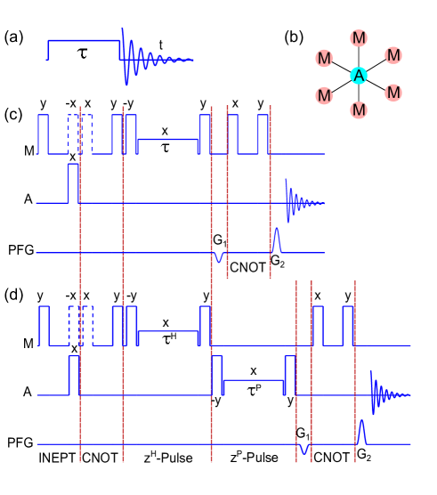
Figure 1: (a) Pulse sequence for single-quantum Torrey oscillation, (b) star-topology spin-systems, (c) pulse sequence for NOON Torrey oscillation, and (d) pulse sequence for the measurement of correlation between two RF channels. In (c) and (d), except the variable duration ($\tau$) pulses, all other pulses are 90^∘ pulses. The operators corresponding to the dashed pulses cancel each other and can be omitted.

Here we describe a method to speed-up the decay of Torrey oscillations using NOON states. NOON states are the highest order multiple-quantum coherences in a given spin-system. Previously, NOON states have been used in NMR for ultra-low magnetic field sensing [7] and for diffusion studies [8].

In the following section we describe the theory of Torrey oscillation, preparation of NOON states, the measurement of RFI using NOON states, and characterization of RFI correlations between two channels of a high resolution NMR probe. The experimental details are described in section 3, and finally we conclude in section 4.

2 Theory

2.1 Radio frequency inhomogeneity

For a given nominal RF amplitude $\nu_{0}$, let us assume RFI distribution $\{\nu,p(\nu)\}$, where $p(\nu)$ is the probability, in the sample volume, of the RF amplitude $\nu$. The mean RF amplitude is $\overline{\nu}=\sum_{\nu}p(\nu)\nu.$ Here we have defined the nominal RF amplitude $\nu_{0}$ as the one with the highest probability. In an asymmetric RFI distribution, $\nu_{0}$ may be different from $\overline{\nu}$.

Consider the standard experiment for estimating RFI via Torrey oscillation as shown in Fig. 1(a). During an on-resonant pulse, the distribution of nutation frequencies $\nu_{1}$ of the single quantum coherence is same as the RFI distribution $p(\nu)$. Therefore real part of the signal collected at the end of a variable-duration ($\tau$) y-pulse is $s(\tau)e^{-t/T_{2}}$, where

$$s(\tau)=\sum_{\nu}p(\nu)\sin(2\pi\nu\tau).$$ (1)

Here $T_{2}$ is the spin-spin relaxation time constant. Similarly, for a $q$-quantum coherence

$$s(\tau)=\sum_{\nu}p(\nu)\sin(2\pi q\nu\tau).$$ (2)

The Fourier transform along $t$ of $s(\tau)e^{-t/T_{2}}$ will result in a Lorentzian of line-width $\pi/T_{2}$ centered at zero frequency (on-resonant case)[9]. The amplitude of this Lorentzian, is proportional to $s(\tau)$. We record a series of experiments by systematically incrementing $\tau$ and obtain the Lorentzian peak-heights $s(\tau)$. In a typical NMR probe, the real part of the Fourier transform

$$S(\nu_{q})={\cal F}_{r}\left[s(\tau)\right]$$ (3)

displays an asymmetric profile, with a maximum at the nominal RF frequency $\nu_{0}$ [3]. This is because in most cases, the probability of finding lower-than-nominal amplitudes is more compared to higher-than-nominal. This profile of RF amplitudes can be modeled by an asymmetric Lorentzian

$$p(\nu) = \frac{\lambda_{1}^{2}}{(1-\frac{\nu}{\nu_{0}})^{2}+\lambda_{1}^{2}}~{}~{}\mathrm{if}~{}~{}\nu<\nu_{0},~{}~{}\mathrm{and,}$$

$$p(\nu) = \frac{\lambda_{2}^{2}}{(1-\frac{\nu}{\nu_{0}})^{2}+\lambda_{2}^{2}}~{}~{}\mathrm{if}~{}~{}\nu\geq\nu_{0}.$$ (4)

The area of $p(\nu)$ is normalized to unity.

Using such a model for RFI it is possible to reconstruct $q$-quantum Torrey oscillations

$$s_{m}(\tau)=\sum_{\nu=0}^{\nu=2\nu_{0}}p(\nu)\sin(2\pi q\nu\tau),$$ (5)

where $\nu$ is the RF frequency with probability $p(\nu)$. The positive real part of the Fourier transform of $s_{m}(\tau)$ gives the model profile $S_{m}(\nu_{q})$. A scalar measure of distance between the model and the experimental profiles is provided by the norm $||S(\nu_{q})-S_{m}(\nu_{q})||$. The RFI parameters $(\lambda_{1},\lambda_{2})$ can be obtained by minimzing the above norm using a non-linear fit.

For the hypothetical case of $\lambda_{1}=\lambda_{2}:=\lambda$, one can model the Torrey oscillation as ${\cal F}^{-1}_{r}\left[S_{m}(\nu_{q})\right]\propto\exp(-\lambda\nu_{0}q\tau).$ Therefore increase in the nominal RF frequency $\nu_{0}$ will correspondingly speed-up the decay of Torrey oscillation. Another way to speedup the decay of Torrey oscillation is to exploit multiple-quantum coherences. In the following we explain how NOON states can be used for efficient characterization of RFI.

2.2 NOON state preparation

We label the Zeeman eigenstates of a single spin-1/2 nucleus as $\left\{|0\rangle,|1\rangle\right\}$. In an $N$-spin system, the NOON state is the superposition of a state $|N,0\rangle$ (with $N$ spins in $|0\rangle$ and $0$ spins in $|1\rangle$) and the state $|0,N\rangle$ (with $0$ spins in $|0\rangle$ and $N$ spins in $|1\rangle$),

$$|N00N\rangle = (|N,0\rangle+|0,N\rangle)/\sqrt{2}$$ (6)

$$= (|00\cdots 0\rangle+|11\cdots 1\rangle)/\sqrt{2}.$$

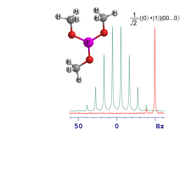
Figure 2: Molecular structure of trimethylphosphite and its ³¹P spectra in equilibrium (upper trace) and after converting NOON state into single quantum coherence (lower trace).

Consider a star-topology spin system as shown in Fig. 1(b). Essentially it is an $AM_{N-1}$ spin system, with a single heteronucleus $A$ interacting with $N-1$ magnetically equivalent $M$ spins via J-coupling. An example system is shown in Fig. 2. The spectrum of $A$ spin is split into $N$ lines, depending on the spin-states of $M_{N-1}$ spins. One of the extreme lines of this spectrum corresponds to the coherence $\frac{1}{\sqrt{2}}(|0\rangle+|1\rangle)|00\cdots 0\rangle$, where each $M$ spin is in the state $|0\rangle$ (see Fig.2). This coherence can be converted into a NOON state  using ${CNOT}$ gates ($NOT$ on all $M$ spins controlled by $A$ spin),

$$\frac{1}{\sqrt{2}}(|0\rangle+|1\rangle)|00\cdots 0\rangle \stackrel{{\scriptstyle CNOT}}{{\longrightarrow}} \frac{1}{\sqrt{2}}(|00\cdots 0\rangle+|11\cdots 1\rangle)=|N00N\rangle.$$ (7)

Since NMR detection is confined to single quantum coherences, it is necessary to convert the NOON state back to single quantum coherence before detection. This can be achieved by the same set of $CNOT$ gates

$$|N00N\rangle\stackrel{{\scriptstyle CNOT}}{{\longrightarrow}}\frac{1}{\sqrt{2}}(|0\rangle+|1\rangle)|00\cdots 0\rangle.$$ (8)

The pulse diagram for NOON state preparation and selection is shown in Fig. 1(c). It can be observed that the $CNOT$ gates in star-topology systems can be implemeted in parallel, and therefore require just two RF pulses on $M$ spins. A pair of PFGs, G₁ and G₂, serve to select the above coherence pathway, and extract the corresponding extreme spectral line (see Fig.2). The PFG ratio

$$\frac{G_{2}}{G_{1}}=(N-1)\frac{\gamma_{M}}{\gamma_{A}}+1,$$ (9)

depends on the size of the spin system ($N$) and the relative gyromagnetic ratio $\gamma_{M}/\gamma_{A}$.

2.3 Measurement of RFI via NOON states

The pulse diagram for the measurement of RFI via NOON states is shown in Fig. 1(c). In order to measure RFI without changing the coherence order of NOON states, we utilize z-pulses. A $\phi_{z}$ pulse acting on a single spin-1/2 system introduces a relative phase shift

$$\frac{1}{\sqrt{2}}(|0\rangle+|1\rangle)\stackrel{{\scriptstyle\phi_{z}}}{{\longrightarrow}}\frac{1}{\sqrt{2}}(|0\rangle+e^{i\phi_{z}}|1\rangle).$$ (10)

If the same pulse is applied on the $M_{N-1}$ spins of a NOON state, and subsequently converted into single quantum coherence, we obtain

$$\frac{1}{\sqrt{2}}(|00\cdots 0\rangle+|11\cdots 1\rangle) \stackrel{{\scriptstyle\phi_{z}^{M}}}{{\longrightarrow}} \frac{1}{\sqrt{2}}(|00\cdots 0\rangle+e^{(N-1)i\phi_{z}}|11\cdots 1\rangle)$$ (11)

$$\stackrel{{\scriptstyle CNOT}}{{\longrightarrow}} \frac{1}{\sqrt{2}}(|0\rangle+e^{i(N-1)\phi_{z}}|1\rangle)|00\cdots 0\rangle.$$

Therefore the resultant phase-shift of the extreme spectral line is $\phi_{z}^{M}=(N-1)\phi_{z}$. A $\phi_{z}^{M}$ pulse, on $M$-spins can be realized by $\left(\frac{\pi}{2}\right)^{M}_{-y}\phi_{x}^{M}\left(\frac{\pi}{2}\right)_{y}^{M}$. Here $\phi_{x}^{M}=2\pi(N-1)\nu_{0}\tau$ is the corresponding x-pulse of duration $\tau$ for a nominal RF amplitude $\nu_{0}$. Ideally, in the absence of RFI, one should see a regular oscillatory behavior of this coherence with $\tau$. In practice we see Torrey oscillation, i.e., decaying oscillations, due to the RFI during $\phi_{x}^{M}$ pulse. As described in section 2.1, NOON Torrey-oscillations in large spin-systems decay much faster than the single-quantum Torrey oscillations. The faster decay of NOON Torrey-oscillations allows one to study RFI at higher amplitudes.

Here RFI of other short and fixed-duration pulses only introduce an over-all scaling factor, and do not contribute to the decay constant of signal. Also, we assumed that the transverse relaxation time constant of NOON state is much longer than the decay constant of NOON Torrey oscillations.

2.4 Correlation between RFI of two channels

In a two-channel probe, the regions of high RF intensity of first channel may not correspond to regions of high RF intensity of the second. In other words, there exists certain correlations between the RFI profiles of the two channels. The NOON state method can be easily extended to study such correlations in the inhomogeneities of two different RF channels. We choose ¹H and ³¹P channels of Bruker QXI probe for studying such correlations and use trimethylphosphite (see Fig. 2) as the star-topology spin system (${}^{31}P^{1}H_{9}$).

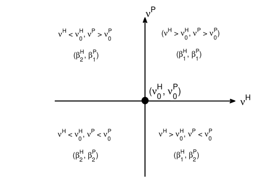
Figure 3: Convention used for selection of $\beta$ parameters of the 3D asymmetric Lorentzian. The central point $(\nu_{0}^{H},\nu_{0}^{P})$ indicates the nominal point, and the four quadrants have different pairs of $\beta$ parameters.

The pulse-diagram for the RFI-correlation study is shown in Fig. 1(d). A $\phi_{z}^{P}$ pulse is introduced after the $\phi_{z}^{H}$ pulse, and the two pulses are independently incremented to obtain a 3D dataset. Similar to Eq. 3, the Fourier transform along the two dimensions result in signal $S(\nu^{H}_{9},\nu^{P}_{1})$. We now model the RFI correlation using a 3D asymmetric Lorentzian:

$$p(\nu^{H},\nu^{P})=\frac{\lambda_{0}^{2}}{d^{2}(\nu^{H},\nu^{P})+\lambda_{0}^{2}},$$ (12)

where $d(\nu^{H},\nu^{P})$ is the scaled distance of $\left(\frac{\nu^{H}}{\nu_{0}^{H}},\frac{\nu^{P}}{\nu_{0}^{P}}\right)$ from the nominal point $(1,1)$:

$$d^{2}(\nu^{H},\nu^{P})=\beta^{H}_{i}\left(1-\frac{\nu^{H}}{\nu^{H}_{0}}\right)^{2}+\beta^{P}_{j}\left(1-\frac{\nu^{P}}{\nu^{P}_{0}}\right)^{2}.$$ (13)

Here $\beta^{H}_{1}$, $\beta^{H}_{2}$, $\beta^{P}_{1}$, and $\beta^{P}_{2}$ are the four asymmetry parameters, on the four quadrants of $\nu^{H}$ - $\nu^{P}$ plane (Fig. 3). The probability distribution is normalized to unit sum.

As described in section 2.1, we first constrcut the model torrey oscillation $s_{m}(\tau^{H},\tau^{P})$ and its Fourier transform $S_{m}(\nu^{H}_{9},\nu^{P}_{1})$. By fitting $S_{m}(\nu^{H}_{9},\nu^{P}_{1})$ with the experimental profile $S(\nu^{H}_{9},\nu^{P}_{1})$, we obtain the best fit parameters $(\lambda_{0},\{\beta\})$.

In the following, we describe experimental characterizations of (i) ¹H RFI at different RF powers in two NMR probes, and (ii) RFI correlation between ¹H and ³¹P channels of a NMR probe.

3 Experiments

The single-quantum Torrey oscillations were studied using a sample consisting of 600 $\upmu$l of 99% D₂O. The NOON Torrey oscillations were studied using 100 $\upmu$l of trimethylphosphite (Fig. 2) dissolved in 500 $\upmu$l of dimethylsulphoxide-D6. The J-couplings between the magnetically equivalent methyl protons and the ³¹P spin are all equal to 11 Hz. The effective T${}_{2}^{*}$ relaxation time constants of ¹H and ³¹P are about 150 ms and 730 ms respectively (as is the general case, T_1ρ is longer than T${}_{2}^{*}$). These values were obtained from respective spectral linewidths. The NOON state T${}_{2}^{*}$ is about 38 ms, and is obtained by introducing a variable delay between the two CNOTs, and then measuring the decay constant of the single quantum coherence after conversion. All the experiments were carried out on a Bruker 500 MHz NMR spectrometer at an ambient temperature of 300 K.

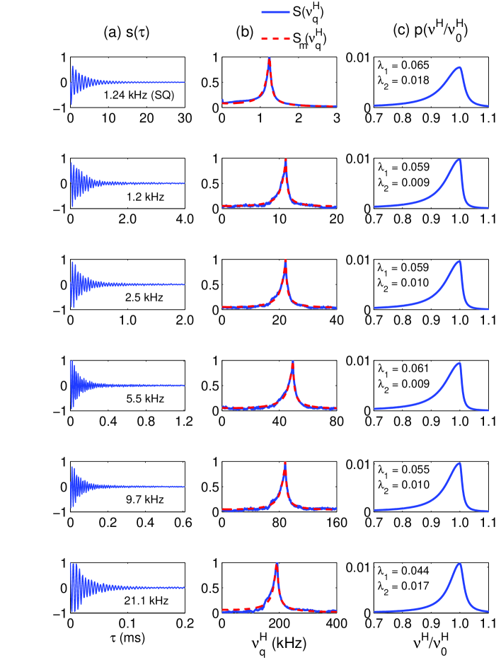
Figure 4: Characterization of RFI in ¹H channel of BBO probe. The results with single quantum method are in the top trace, and other traces are for NOON states with different nominal RF amplitudes (as indicated in column (a)). Column (a): Torrey oscillations s($\tau$) vs $\tau$. Column (b): Positive real part of Fourier transform $S(\nu^{H}_{q})$ vs $\nu_{q}^{H}$ (solid lines). Also shown are the best fits with model $S_{m}(\nu^{H}_{q})$ (dashed lines). Column (c): The RFI profiles p($\nu^{H}/\nu_{0}^{H}$) vs $\nu^{H}/\nu_{0}^{H}$. The asymmetric linewidth parameters $(\lambda_{1},\lambda_{2})$ are indicated in each case.

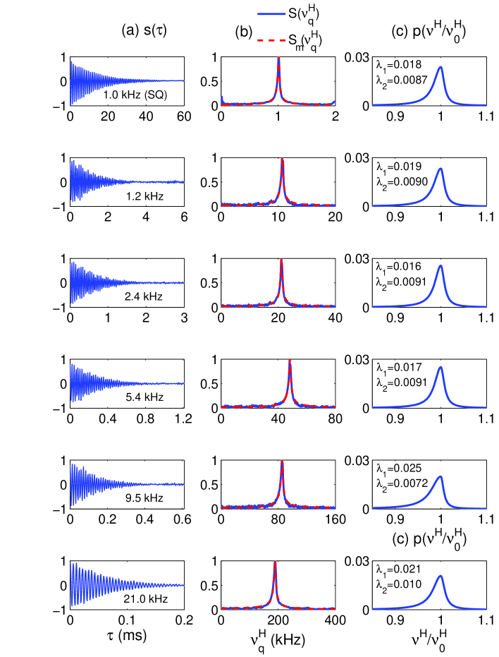
Figure 5: Characterization of RFI in ¹H channel of QXI probe. The results with single quantum method are in the top trace, and other traces are for NOON states with different nominal RF amplitudes (as indicated in column (a)). Column (a): Torrey oscillations s($\tau$) vs $\tau$. Column (b): Positive real part of Fourier transform $S(\nu^{H}_{q})$ vs $\nu_{q}^{H}$ (solid lines). Also shown are the best fits with model $S_{m}(\nu^{H}_{q})$ (dashed lines). Column (c): The RFI profiles p($\nu^{H}/\nu_{0}^{H}$) vs $\nu^{H}/\nu_{0}^{H}$. The asymmetric linewidth parameters $(\lambda_{1},\lambda_{2})$ are indicated in each case.

3.1 RFI characterization of ¹H channel

The single quantum Torrey oscillations were studied using the pulse sequence shown in Fig. 1(a). A series of spectral lines were recorded by incrementing the duration of the low-power (about 1 kHz) on-resonant pulse on 99% D₂O sample as described in section 2.1. The results of the single quantum experiments on ¹H channels of BBO and QXI probes are shown in the top trace of Figs. 4 and 5 respectively. The nominal RF frequencies were found to be slightly different for the two probes as indicated in the figures. The $\tau$-increments in BBO and QXI were set to 112.5 $\upmu$s and 250 $\upmu$s respectively, and a total of 256 transients were recorded. The Torrey oscillation ($s(\tau)$), the positive real part of the Fourier transform ($S(\nu_{1}^{H})$) are shown in the first traces of Figs. 4(a,b) and 5(a,b). By fitting the model $S_{m}(\nu_{1}^{H})$ to $S(\nu_{1}^{H})$, we obtain the asymmetry parameters $\lambda_{1}$ and $\lambda_{2}$ and the corresponding RFI profile $p(\nu^{H})$. The top traces of Figs. 4(c) and 5(c) show the RFI profiles $p(\nu^{H})$ and the corresponding $\lambda$ values for BBO and QXI probes respectively.

The NOON state is prepared with the ³¹P-¹H₉ system of trimethylphosphite (Fig. 2) using the pulse sequence shown in Fig. 1(c). The results of the NOON Torrey oscillations at different nominal amplitudes of ¹H channels of BBO and QXI probes are shown in Figs. 4(a) and 5(a). It can be observed that as the nominal amplitude is increased, the Torrey oscillations decay faster. The positive real parts of the Fourier transform $S(\nu_{9}^{H})$ of the 9-quantum Torrey oscillations are shown in Figs. 4(b) and 5(b). By fitting the model function $S_{m}(\nu^{H}_{9})$ to $S(\nu_{9}^{H})$ at each of these nominal amplitudes, we obtained the corresponding RFI profiles $p(\nu^{H})$. These profiles and the asymmetry parameters $(\lambda_{1},\lambda_{2})$ are shown in Figs. 4(c) and 5(c).

It can be observed that decay times of the NOON state Torrey oscillations are an order of magnitude shorter than the single quantum Torrey oscillations in both probes. This fact allowed us to characterize RFI safely even at maximum allowed RF powers. The excellent fit in all the cases indicates the validity of our model. In the overall comparison, we find that the BBO probe has stronger RFI than QXI probe at all RF amplitudes. The mean values of $(\lambda_{1},\lambda_{2})$ are (0.057,0.012) and (0.019,0.009) respectively in BBO and QXI probes.

In QXI probe, the RFI profiles are not only sharper than those in BBO, but are also more symmetric. The mean ratios $\lambda_{1}/\lambda_{2}$ are 5.2 and 2.2 in BBO and QXI respectively. QXI probe shows some what stronger RFI at higher RF amplitudes. For example, RFI profiles at 9.5 kHz and 21 kHz are significantly wider than the profile at 5.4 kHz.

3.2 RFI correlation between ¹H and ³¹P channels

We measured RFI correlation between ¹H and ³¹P channels of Bruker QXI probe using the NOON state method. The pulse sequence for measuring RFI correlation between ¹H and ³¹P channels is shown in Fig. 1(d) and the theory is described in section 2.4. The dataset of 2D Torrey oscillations was recorded by independently incrementing the $\tau^{H}$ and $\tau^{P}$ pulses respectively by 11.1 $\upmu$s and 50.0 $\upmu$s. The nominal RF amplitudes in ¹H and ³¹P channels were 2.4 kHz and 2.5 kHz respectively. A total of 128 data points in ¹H dimension and 96 data points in ³¹P dimension were collected. The real positive part of the Fourier transform of the 2D Torrey oscillations $S(\nu^{H}_{9},\nu^{P}_{1})$ was obtained after a zero-fill to 256 points in each dimension. The contour plot of $S(\nu^{H}_{9},\nu^{P}_{1})$ is shown in Fig. 6(a). The asymmetric Lorentzian parameters $(\lambda_{0},\{\beta\})$ were obtained by fitting the model profile $S_{m}(\nu^{H}_{9},\nu^{P}_{1})$ to $S(\nu^{H}_{9},\nu^{P}_{1})$. Fig. 6(b) displays $S_{m}(\nu^{H}_{9},\nu^{P}_{1})$ corresponding to the best fit: $\{\lambda_{0}=0.0045,\beta_{1}^{H}=0.114,\beta_{2}^{H}=0.226,\beta_{1}^{P}=0.095,\beta_{2}^{P}=0.028\}$. It can be seen that the model profile $S_{m}(\nu^{H}_{9},\nu^{P}_{1})$ approximates the overall profile of $S(\nu^{H}_{9},\nu^{P}_{1})$. The corresponding RFI profile $p(\nu^{H},\nu^{P})$ is shown in Fig. 6(c). It can be observed that ³¹P-channel has a wider RFI distribution than the ¹H-channel.

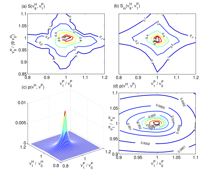
Figure 6: Characterization of RFI correlations between ¹H and ³¹P channels of QXI probe. (a) Contour plot showing real positive part of Fourier transform of 2D Torrey oscillations $S(\nu^{H}_{9},\nu_{1}^{P})$, (b) corresponding simulated profile obtained with the best fit model $S_{m}(\nu^{H}_{9},\nu_{1}^{P})$, (c) the surface plot of the RFI profile $p(\nu^{H},\nu^{P})$, and (d) the contour plot of $p(\nu^{H},\nu^{P})$.

4 Conclusions

We have proposed an asymmetric Lorentzian model to describe radio-frequency inhomogeneity. Using this model, we obtained the asymmetric line-width parameters in two high-resolution NMR probes using single quantum Torrey oscillations. The excellent fit between the experimental profile and the simulated profile indicated the suitability of the asymmetric Lorentzian model.

We have described the characterization of RFI using NOON states. NOON state Torrey oscillations decay much faster than single quantum Torrey oscillations allowing the characterization of RFI at higher RF amplitudes. Using this method, we have studied RFI of two NMR probes at different RF amplitudes and compared the results. We have also proposed a 3D Lorentzian model to describe RFI correlations between two RF channls. Then we extended the NOON state method to characterize such correlations, and demonstrated it on ¹H-³¹P channels. We believe that these characterizations will be useful to design high-precision NMR and MRI experiments as well as to design high-fidelity quantum gates required in NMR quantum information processing.

References

- [1] M. H. Levitt, Spin dynamics, John Wiley & sons, Ltd. Chichester, England, 2002.
- [2] J. Cavanagh, W. J. Fairbrother, A. J. Palmer III, M. Rance, and N. J. Skelton, Protein NMR Spectroscopy: Principles and practice, Elesveir Acadmic Press, Burlington, USA, 2007.
- [3] M. A. Pravia, N. Boulant and J. Emerson, A. Farid, E. M. Fortunato, T. F. Havel, R. Martinez, and D. G. Cory. Robust control of quantum information, J. chem. phys. 119 (2003) 9993-10001.
- [4] M. A. Oghabian, N. R. Alam, and S. Mehdipour, A new method for measurement of Radio Frequency Inhomogeinity in MRI, Iran. J. Of radiology 1 (2003) 113-119.
- [5] B. R. Condon, J. Patterson, D. Wyper, A. Jenkins, and D. M. Hadley, Image nonuniformity in magnetic resonance imaging: its magnitude and methods for its correction, The British J. of Radiology 60 (1987) 83-87.
- [6] H. C. Torrey, Transient Nutations in Nuclear Magnetic Resonance, phys. rev. 76 (1949) 1059-1068.
- [7] J. A. Jones, S. D. Karlen, J. Fitzsimons, A. Ardavan, S. C. Benjamin, G. A. D. Briggs, and J. J. L. Morton, Magnetic Field Sensing Beyond the Standard Quantum Limit Using 10-Spin NOON States, Science 324 (2009) 1166-1168.
- [8] A. Shukla, M. Sharma, and T. S. Mahesh, e-print arXiv:1110.1481 (2011).
- [9] H. J. Weber, G. B. Arfken, Essential Mathematical Methods for Physicists, Elseveir Acadmic Press, california, USA, 2004.