On Training Deep Boltzmann Machines

Abstract

The deep Boltzmann machine (DBM) has been an important development in the quest for powerful “deep” probabilistic models. To date, simultaneous or joint training of all layers of the DBM has been largely unsuccessful with existing training methods. We introduce a simple regularization scheme that encourages the weight vectors associated with each hidden unit to have similar norms. We demonstrate that this regularization can be easily combined with standard stochastic maximum likelihood to yield an effective training strategy for the simultaneous training of all layers of the deep Boltzmann machine.

1 Introduction

Since its introduction by Salakhutdinov and Hinton [7], the deep Boltzmann machine (DBM) has been one of the most ambitious attempts to build a probabilistic model with many layers of latent or hidden variables. The DBM shares some characteristics with the earlier deep belief network (DBN) [3]. Both models may be viewed as multi-layer or “deep” extensions of the popular restricted Boltzmann machine (RBM). However, unlike the DBN, commonly used DBM approximate inference schemes implement true feedback mechanisms where the inferred activations of high-level units can influence the activations of lower-level units. Thus alternative interpretations of an input are able to compete at all levels of the model simultaneously. This sort of sophistication in inference has the potential to lead to more robust and globally coherent inferences, which are likely to translate to better performance when the model is employed in tasks such as classification.

Despite its success, the DBM has not yet entirely fulfilled this potential and the DBN remains the more popular model paradigm for deep probabilistic models. One potential explanation of why this is so could be tied to the difficulties one encounters when attempting to estimate the model parameters from data. Straightforward applications of gradient-based methods such as stochastic maximum likelihood (SML) [10] (also known as persistent contrastive divergence [9]) appear to fall in poor local minima, and fail to adequately explore the space of model parameters.

One solution, as presented in [7], is based on a greedy layer-wise pretraining strategy which appears to overcome these poor local minima . Each layer is trained as an RBM with the latent activations of the layer below as its input. These layers are then recombined by rescaling the weights to account for the doubling of inputs into each intermediate layer. While this procedure seems to work well, it involves many steps and is more complicated than would be ideal. Also, more importantly, the necessity of layer-wise pretraining makes it very difficult for the organization of upper layers to influence the topological organization of lower layers. For example, in cases where we would like to learn a DBM that is not fully connected between each layer, it would potentially be very desirable for the global connectivity pattern (eg. local receptive fields) to influence the pattern of learned filters at all layers. Layer-wise pretraining precludes this possibility. If, on the other hand, one could jointly train all layers of a deep Boltzmann machine simultaneously, then the pattern of activation of the upper layer units would have an opportunity to influence the weights trained at the lower layers via their effect on lower-layer units activations.

In this paper, we describe a simple scheme for joint training of all layers of a deep Boltzmann machine. Our strategy is based on the observation that the poor local minima in which SML falls are characterized by high variance in the norms of the weight vectors, particularly those between the data and the first layer of hidden units. Our solution is to simply add a regularization term to the standard maximum likelihood training criterion that penalizes large differences in the norms of the weight vectors, both within a layer and across neighbouring layers. Our regularization is based on the intuition that successful models are those where all units contribute roughly equally to the representation of the data. This is a common principle that has previously been applied in the form of sparsity penalties for RBM and DBN training [5], where all hidden units are encouraged to be active over an equal proportion of the data. Our application of this principal is somewhat different, we do not explicitly control the activation of the hidden units, instead we encourage equal influence of each active hidden unit. We demonstrate, with experiments, both the failure of standard SML training for DBMs and the effectiveness of our regularized-SML DBM training strategy.

2 Boltzmann Machines

A Boltzmann machine is defined as a network of symmetrically-coupled binary stochastic units (random variables). These stochastic units can be divided into two groups: (1) the visible units $v\in\{0,1\}^{D}$ that represent the data, and (2) the hidden units $h\in\{0,1\}^{N}$ that mediate dependencies between the visible units through their mutual interactions. The pattern of interaction is specified through the energy function:

$$E_{\mathrm{BM}}(v,h;\theta)=-\frac{1}{2}v^{T}Uv-\frac{1}{2}h^{T}Vh-v^{T}Wh-b^{T}v-d^{T}h,$$ (1)

where $\theta=\{U,V,W,b,d\}$ are the model parameters which respectively encode the visible-to-visible interactions, the hidden-to-hidden interactions, the visible-to-hidden interactions, the visible self-connections, and the hidden self-connections (also known as biases). To avoid over-parametrization, the diagonals of $U$ and $V$ are set to zero.

The energy function specifies the probability distribution over the joint space $[v,h]$, via the Boltzmann distribution:

$$P(v,h)=\frac{1}{Z(\theta)}\exp\left(-E_{\mathrm{BM}}(v,h;\theta)\right),$$ (2)

where the partition function $Z(\theta)$ ensures that the density normalizes:

$$Z(\theta)=\sum_{v_{1}=0}^{v_{1}=1}\cdots\sum_{v_{D}=0}^{v_{D}=1}\sum_{h_{1}=0}^{h_{1}=1}\cdots\sum_{h_{N}=0}^{h_{N}=1}\exp\left(-E_{\mathrm{BM}}(v,h;\theta)\right).$$ (3)

This joint probability distribution gives rise to the set of conditional distributions of the form:

$$P(h_{i}\mid v,h_{\setminus i}) = \mathrm{sigmoid}\left(\sum_{j}W_{ji}v_{j}+\sum_{i^{\prime}\setminus i}V_{ii^{\prime}}h_{i^{\prime}}+d_{i}\right)$$ (4)

$$P(v_{j}\mid h,v_{\setminus j}) = \mathrm{sigmoid}\left(\sum_{i}W_{ji}v_{j}+\sum_{j^{\prime}\setminus j}U_{jj^{\prime}}v_{j^{\prime}}+b_{j}\right).$$ (5)

In general, inference in the Boltzmann machine is intractable. For example, computing the conditional probability of $h_{i}$ given the visibles, $P(h_{i}\mid v)$, requires marginalizing over the rest of the hiddens which implies evaluating a sum with $2^{N-1}$ terms:

$$P(h_{i}\mid v)=\sum_{h_{1}=0}^{h_{1}=1}\cdots\sum_{h_{i-1}=0}^{h_{i-1}=1}\sum_{h_{i+1}=0}^{h_{i+1}=1}\cdots\sum_{h_{N}=0}^{h_{N}=1}P(h\mid v)$$ (6)

However with some judicious choices in the pattern of interactions between the visible and hidden units, more tractable subsets of the model family are possible.

2.1 Restricted Boltzmann Machines

The restricted Boltzmann machine (RBM) is likely the most popular subset of Boltzmann machines. They are defined by restricting the interactions in the Boltzmann energy function, in Eq. 10, to only those between $h$ and $v$, i.e. for $E_{\mathrm{RBM}}$, $U=\mathbf{0}$ and $V=\mathbf{0}$. As such, the RBM can be said to form a bipartite graph with the visibles and the hiddens forming two layers of vertices in the graph. With this restriction, the RBM possesses the useful property that the conditional distribution over the hidden units factorizes given the visibles:

$$P(h\mid v)=\prod_{i}P(h_{i}\mid v)=\prod_{i}\mathrm{sigmoid}\left(\sum_{j}W_{ji}v_{j}+d_{i}\right)$$ (7)

Likewise, the conditional distribution over the visible units given the hiddens also factorizes:

$$P(v\mid h)=\prod_{j}P(v_{j}\mid h)=\prod_{j}\mathrm{sigmoid}\left(\sum_{i}W_{ji}h_{i}+b_{j}\right)$$ (8)

This conditional factorization property of the RBM immediately implies that most inferences we would like make are readily tractable. For example, the conditional independence of the hiddens implies that posterior marginals of the form $P(h_{i}\mid v)$ are immediately available.

Importantly, the tractability of the RBM does not extend to its partition function, which still involves sums with exponential number of terms. It does imply however that we can limit the number of terms to $\min\{2^{D},2^{N}\}$. Usually this is still an unmanageable number of terms and therefore we must resort to approximate methods to deal with its computation.

Learning in the RBM is also rendered much more tractable in comparison to the general Boltzmann machine. Typically, learning involves finding a set of model parameters that approximately maximizes the log likelihood of a training dataset:

$$\sum_{t}logP(v_{:,t};\theta)=\sum_{t}log\sum_{h_{1,t}=0}^{h_{1,t}=1}\cdots\sum_{h_{N,t}=0}^{h_{N,t}=1}P(v_{:,t},h_{:,t};\theta).$$ (9)

This can be accomplished via gradient ascent. The gradient of the log likelihood of the data for the RBM is given by:

$$\frac{\partial}{\partial\theta_{i}}\left(\sum_{t=1}^{T}\log p(v_{:,t})\right)=-\sum_{t=1}^{T}\left\langle\frac{\partial}{\partial\theta_{i}}E_{\mathrm{RBM}}(v_{:,t},h)\right\rangle_{p(h_{:,t}\mid v_{:,t})}+\sum_{t=1}^{T}\left\langle\frac{\partial}{\partial\theta_{i}}E_{\mathrm{RBM}}(v,h)\right\rangle_{p(v,h)},$$

where we have the expectations with respect to $p(h_{:,t}\mid v_{:,t})$ in the “clamped” condition, and over the full joint $p(v_{:,t},h_{:,t})$ in the “unclamped” condition. In training, we follow the stochastic maximum likelihood (SML) algorithm (also know as persistent contrastive divergence or PCD) [10, 9], i.e., performing only one or a few updates of an MCMC chain between each parameter update.

3 Deep Boltzmann Machines

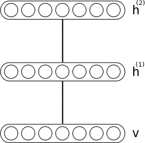
Figure 1: A graphical depiction of a 2-layer DBM. Undirected weights connect the visible layer to layer $h^{(1)}$; and layers $h^{(1)}$ to $h^{(2)}$. Note that $v$ and $h^{(2)}$ are conditionally independent given $h^{(1)}$.

The Deep Boltzmann Machine (DBM) is another particular subset of the Boltzmann machine family of models where the units are again arranged in layers. However unlike the RBM, the DBM possesses multiple layers of hidden units as illustrated in Figure 1. With respect to the Boltzmann energy function of Eq. 10, the DBM corresponds to setting $U=0$ and a sparse connectivity structure in both $V$ and $W$. We can make the structure of the DBM more explicit by specifying its energy function. For the 2-layer model it is given as:

$$E_{\mathrm{DBM}}(v,h^{(1)},h^{(2)};\theta)=-v^{T}Wh^{(1)}-\left.h^{(1)}\right.^{T}Vh^{(2)}-\left.d^{(1)}\right.^{T}h^{(1)}-\left.d^{(2)}\right.^{T}h^{(2)}-b^{T}v,$$ (10)

with $\theta=\{W,V,d^{(1)},d^{(1)},b\}$. The DBM can also be characterized as a bipartite graph between two sets of vertices, formed by the units in odd and even-numbered layers (with $v:=h^{(0)}$).

3.1 Mean-field approximate inference

A key point of departure from the RBM is that the posterior distribution over the hidden units (given the visibles) is no longer tractable, due to the interactions between the hidden units. Salakhutdinov and Hinton [7] resort to a mean-field approximation to the posterior. Specifically, in the case of the 2-layer model, we wish to approximate $P\left(h^{(1)},h^{(2)}\mid v\right)$ with the factored distribution $Q_{v}(h^{(1)},h^{(2)})=\prod_{j=1}^{N_{1}}Q_{v}\left(h^{(1)}_{j}\right)\ \prod_{i=1}^{N_{2}}Q_{v}\left(h^{(2)}_{i}\right)$. such that the KL divergence $\mathrm{KL}\left(P\left(h^{(1)},h^{(2)}\mid v\right)\|Q_{v}(h^{1},h^{2})\right)$ is minimized or equivalently, that a lower bound to the log likelihood is maximized:

$$\log P(v)>\mathcal{L}(Q_{v})\equiv\sum_{h^{(1)}}\sum_{h^{(2)}}Q_{v}(h^{(1)},h^{(2)})\log\left(\frac{P(v,h^{(1)},h^{(2)})}{Q_{v}(h^{(1)},h^{(2)})}\right)$$ (11)

Maximizing this lower-bound with respect to the mean-field distribution $Q_{v}(h^{1},h^{2})$ yields the following mean field update equations:

$$\hat{h}^{(1)}_{i} \leftarrow\mathrm{sigmoid}\left(\sum_{j}W_{ji}v_{j}+\sum_{k}V_{ik}\hat{h}^{(2)}_{k}+d^{(1)}_{i}\right)$$ (12)

$$\hat{h}^{(2)}_{k} \leftarrow\mathrm{sigmoid}\left(\sum_{i}V_{ik}\hat{h}^{(1)}_{i}+d^{(2)}_{k}\right)$$ (13)

Iterating Eq. (12-13) until convergence yields the parameters used to estimate the “variational positive phase” of Eq. 14:

$$\mathcal{L}(Q_{v}) =\mathbb{E}_{Q_{v}}\left[\log P(v,h^{(1)},h^{(2)})-\log Q_{v}(h^{(1)},h^{(2)})\right]$$

$$=\mathbb{E}_{Q_{v}}\left[-E_{\mathrm{DBM}}(v,h^{(1)},h^{(2)})-\log Q_{v}(h^{(1)},h^{(2)})\right]-\log Z(\theta)$$

$$\frac{\partial\mathcal{L}(Q_{v})}{\partial\theta} =-\mathbb{E}_{Q_{v}}\left[\frac{\partial E_{\mathrm{DBM}}(v,h^{(1)},h^{(2)})}{\partial\theta}\right]+\mathbb{E}_{P}\left[\frac{\partial E_{\mathrm{DBM}}(v,h^{(1)},h^{(2)})}{\partial\theta}\right]$$ (14)

Note that this variational learning procedure leaves the “negative phase” untouched. It can thus be estimated through SML or Contrastive Divergence [2] as in the RBM case.

3.2 Training Deep Boltzmann Machines

Despite the intractability of inference in the DBM, its training should not, in theory, be much more complicated than that of the RBM. The major difference being that instead of maximizing the likelihood directly, we instead choose parameters to maximize the lower-bound on the likelihood given in Eq. 11. The SML-based algorithm for maximizing this lower-bound is as follows:

1. Clamp the visible units to a training example.

2. Iterate over Eq. (12-13) until convergence.

3. Generate negative phase samples $v^{-}$, $h^{(1)-}$ and $h^{(2)-}$ through SML.

4. Compute $\partial\mathcal{L}(Q_{v})\left/\partial\theta\right.$ using the values obtained in steps 2-3.

5. Finally, update the model parameters with a step of gradient ascent.

While the above procedure appears to be a simple extention of the highly effective SML scheme for training RBMs, as we demonstrate in Sec. 5, this procedure seems vulnerable to falling in poor local minima which leave many filters effectively dead (not significantly different from its random initialization with small norm).

The failure of the SML joint training strategy was noted by Salakhutdinov and Hinton [7]. As a far more successful alternative, they proposed a greedy layer-wise training strategy. This procedure consists in pre-training the layers of the DBM, in much the same way as the Deep Belief Network: i.e. by stacking RBMs and training each layer to independently model the output of the previous layer. A final joint “fine-tuning” is done following the above SML-based procedure.

4 Joint Training of a DBM

While greedy layer-wise training has been shown to be reasonably successful, a means of joint training a DBM would be highly desireable. Not only would it be simpler, but it would open the door to local receptive field learning and more general architectures where we would like the top-down pattern of connectivity to influence the learning of lower-level features. In this section we detail our simple proposal for a means to jointly train all layers of a DBM.

Our strategy is based on the observation that standard SML-based joint training tends produce high variance in the weight vectors associated with each hidden unit – particularly across the first-layer weight vectors that connect the visible units to the first hidden layer units.

Our proposal is thus to regularize the maximum likelihood objective, in order to encourage units to have similar norms (i) within a given layer and (ii) to a lesser extent, across neighbouring layers. We thus introduce an additional parameter $\mu^{(l)}$ for each layer of the DBM, representing the average norm of weight vectors of the $l$-th layer. We then add a regularization term to our objective $\mathcal{L}(Q_{v})$, which penalizes deviations from this mean-value using a squared-error penalty. $\mu^{(l)}$’s belonging to adjacent layers are further constrained to be close (again in the $l2$ sense). This gives rise to the following regularized objective:

$$\max_{\theta}\mathcal{L}(Q_{v})+\ \alpha^{(1)}\sum_{j=1}^{N_{1}}\left(\|W_{\cdot i}\|_{2}-\mu^{(1)}\right)^{2}+\ \alpha^{(2)}\sum_{i=1}^{N_{2}}\left(\|V_{\cdot j}\|_{2}-\mu^{(2)}\right)^{2}+\ \gamma\left(\mu^{(1)}-\mu^{(2)}\right)^{2}.$$ (15)

One can think of this regularization term as a spring, which ensures that the system evolves jointly from an initial random weight configuration (where the columns of $W^{(l)}$ have small norm) to a good model of the input distribution $P(v)$, which undoubtedly requires weight vectors with larger norms.

5 Experiments

To evaluate the effect of our regularization term, we trained deep Boltzmann machines on the pervasive MNIST dataset [4]. All our models were trained for $10^{6}$ updates, using minibatches of size $50$, varying the learning rate in $\{10^{-2},10^{-3},10^{-4}\}$.

Direct Approach

Our first model was a 3-layer DBM with [500,500,1000] hidden units in the first, second and third layers (respectively). The resulting filters are shown in Figure 2.

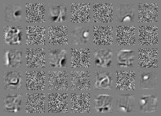
(a) Layer 1

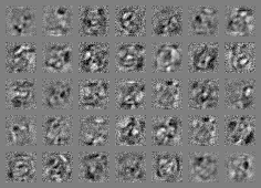
(b) Layer 2

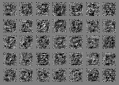
(c) Layer 3

Figure 2: Random subset of filters obtained by a 784-500-500-1000 DBM, after $10^{6}$ updates (trained jointly, using the direct approach). The learning rate was set to $10^{-3}$ and the batch size to $50$. Higher-level weights are visualized by performing a linear combination of lower-level weights, but only picking the $20$ most active connections.

As we can see, many of the first-layer filters are not significantly different from their random initialization, with very small norm. Based on the difference between these results and the successful training of an RBM, we speculate that the top-down interactions prevent the first layer from learning useful filters. We have confirmed that the high-frequency “noise” filters are actually the ones with lowest norm. It seems as though early top-down input is influencing the activations of these hidden units, perhaps directly through some form of suppression, or indirectly, by reinforcing the activation of the subset of filters which become useful early on. While we plot filters for 3-layer networks, the same results hold for networks of depth two.

Joint Training

Using our regularized objective, we train a 2-layer DBM with 500 hidden units in each layer. We set the hyper-parameters of Eq.15 as follows: $\alpha^{(1)}=0.1$, $\alpha^{(2)}=0.1$ and $\gamma=1$. Furthermore, we dampen the learning rate on the parameters $\mu^{(1)}$ and $\mu^{(2)}$ by a factor of a thousand, in order for the layer norms to evolve more slowly. A random subset of filters is shown in Figure 3.

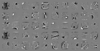
(a) Layer 1

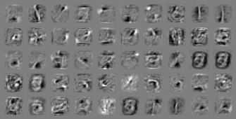
(b) Layer 2

Figure 3: Random subset of filters obtained by a 784-500-500 DBM, after $10^{6}$ updates. All layers were trained jointly using the regularized cost of Eq.15. The learning rate was set to $10^{-2}$ and the batch size to $50$.

The effect of our regularization term is drastic: the vast majority of first layer filters seem to train successfully and resemble the pen-stroke detectors characteristic of features learned on MNIST. While more difficult to interpret, the second layer filters are also clearly superior to the ones of Figure 2, combining lower-level features (pen strokes) into more global digit-like objects.

6 Discussion

We have introduced a simple regularization scheme that appears to prevent SML from falling into a poor local minimum of our objective function. The regularizer encourages units to learn filters which have similar norms, both within and across adjacent layers. We have empirically demonstrated the failure of joint training of all layers of a deep Boltzmann machine which leaves many filters in the lower layer of a 2-layer DBM with very small norm and, consequently, little contribution to modeling the data. We have also empirically demonstrated the success of our regularization scheme in simultaneously training both layers of a 2-layer DBM. While we have not shown it here, our scheme also appears to work well for DBMs with more than 2 layers. In future work, we would like to determine how many layers can be learnt simultaneously using similar basic norm-regularizaiton schemes.

Acknowledgments

The authors would like to acknowledge the support of the following agencies for research funding and computing support: NSERC, Calcul Québec and CIFAR. We would also like to thank the developers of Theano [1].

References

- Bergstra et al. [2010] Bergstra, J., Breuleux, O., Bastien, F., Lamblin, P., Pascanu, R., Desjardins, G., Turian, J., Warde-Farley, D., and Bengio, Y. (2010). Theano: a CPU and GPU math expression compiler. In Proceedings of the Python for Scientific Computing Conference (SciPy). Oral Presentation.
- Hinton [2000] Hinton, G. E. (2000). Training products of experts by minimizing contrastive divergence. Technical Report GCNU TR 2000-004, Gatsby Unit, University College London.
- Hinton et al. [2006] Hinton, G. E., Osindero, S., and Teh, Y. (2006). A fast learning algorithm for deep belief nets. Neural Computation, 18, 1527–1554.
- LeCun et al. [1998] LeCun, Y., Bottou, L., Bengio, Y., and Haffner, P. (1998). Gradient based learning applied to document recognition. IEEE, 86(11), 2278–2324.
- Lee et al. [2008] Lee, H., Ekanadham, C., and Ng, A. (2008). Sparse deep belief net model for visual area V2. In NIPS’07, pages 873–880. MIT Press, Cambridge, MA.
- Neal [2001] Neal, R. M. (2001). Annealed importance sampling. Statistics and Computing, 11(2), 125–139.
- Salakhutdinov and Hinton [2009] Salakhutdinov, R. and Hinton, G. (2009). Deep Boltzmann machines. In Proceedings of the Twelfth International Conference on Artificial Intelligence and Statistics (AISTATS 2009), volume 8.
- Salakhutdinov and Murray [2008] Salakhutdinov, R. and Murray, I. (2008). On the quantitative analysis of deep belief networks. In W. W. Cohen, A. McCallum, and S. T. Roweis, editors, ICML 2008, volume 25, pages 872–879. ACM.
- Tieleman [2008] Tieleman, T. (2008). Training restricted Boltzmann machines using approximations to the likelihood gradient. In W. W. Cohen, A. McCallum, and S. T. Roweis, editors, ICML 2008, pages 1064–1071. ACM.
- Younes [1999] Younes, L. (1999). On the convergence of markovian stochastic algorithms with rapidly decreasing ergodicity rates. Stochastics and Stochastic Reports, 65(3), 177–228.