Analysis of Sparse MIMO Radar

Abstract

We consider a multiple-input-multiple-output radar system and derive a theoretical framework for the recoverability of targets in the azimuth-range domain and the azimuth-range-Doppler domain via sparse approximation algorithms. Using tools developed in the area of compressive sensing, we prove bounds on the number of detectable targets and the achievable resolution in the presence of additive noise. Our theoretical findings are validated by numerical simulations.

Keywords: Sparsity, Radar, Compressive Sensing, Random Matrix, MIMO

1 Introduction

While radar systems have been in use for many decades, radar is far from being a ‘solved problem’. Indeed, exciting new developments in radar pose great challenges both to engineers and mathematicians [6]. Two such developments are the advent of MIMO (multi-input multi-output) radar [10], and the application of compressed sensing to radar signal processing [15].

MIMO radar is characterized by using multiple antennas to simultaneously transmit diverse, usually orthogonal, waveforms in addition to using multiple antennas to receive the reflected signals. MIMO radar has the potential for enhancing spatial resolution and improving interference and jamming suppression. The ability of MIMO radar to shape the transmit beam post facto allows for adapting the transmission based on the received data in a way which is not possible in non-MIMO radar.

A radar system illuminates a given area and attempts to detect and determine the location of objects of interest in its field of view, and to estimate their strength (radar reflectivity). The space of interest may be divided into range-azimuth (distance and direction) cells, or range-Doppler-azimuth (distance, direction and speed) cells in the case there is relative motion between the radar and the object. In many cases the radar scene is sparse in the sense that only a small fraction (often a very small fraction) of the cells is occupied by the objects of interest.

Conventional radar processing does not take into account the a-priori knowledge that the radar scene is sparse. Recent works, such as [15, 21] developed techniques which attempt to exploit this sparsity using tools from the area of compressed sensing [4, 8]. The exploitation of sparsity has the potential to improve the performance of radar systems under certain conditions and is therefore of considerable practical interest.

In this paper we study the issue of sparsity in the specific context of a MIMO radar system employing multiple antennas at the transmitter the receiver, where the two arrays are co-located. We note that related work on the application of compressive sensing techniques to MIMO radar can be found in [30, 31]. Our emphasis here is on developing the basic theory needed to apply sparse recovery techniques for the detection of the locations and reflectivities of targets for MIMO radar.

The basic model for the problem we are considering involves a linear measurement equation ${\bf y}={\bf A}{\bf x}+{\bf w}$ where ${\bf y}$ is a vector of measurements collected by the receiver antennas over an observation interval, ${\bf A}$ is a measurement matrix whose columns correspond to the signal received from a single unit-strength scatterer at a particular range-azimuth (or range-azimuth-Doppler) cell, ${\bf x}$ is a vector whose elements represent the complex amplitudes of the scatterers, and ${\bf w}$ is a noise vector. The measurement equation is assumed to be under-determined, possibly highly under-determined. The sparsity of the radar scene is introduced by assuming that only $K$ elements of the vector ${\bf x}$ are non-zero, where $K$ is much smaller than the dimension of the vector. The measurement matrix ${\bf A}$ embodies in it the details of the radar system such as the transmitted waveforms and the structure of antenna array.

In this paper we study the conditions under which this problem has a satisfactory solution. This is a fundamental issue of both theoretical and practical importance. More specifically, the analysis presented in the following sections addresses the following issues:

• It is known from the theory of compressed sensing [4, 8] that the matrix ${\bf A}$ must satisfy certain conditions in order that the solution computed via an appropriate convex program will indeed coincide with the desired sparsest solution (whose computation is in general an NP-hard problem). In our problem the characteristics of this matrix depend on the choice of the radar waveforms and the number and positions of the transmit and receive antennas. We develop the results necessary for understanding how the selection of the parameters of the radar system affects the conditions mentioned above.

• The ability of the algorithm to correctly detect targets depends on the number of these targets, $K$, and the signal to noise ratio. We show that as long as the number of the targets is less than a maximal value $K_{\max}$, and the signal to noise is larger than some minimal value ${\rm SNR}_{\min}$, the targets can be correctly detected with high probability by solving an $\ell_{1}$-regularized least squares problem known under the name lasso. Explicit formulas are presented for $K_{\max}$ and ${\rm SNR}_{\min}$ as a function of the number of transmit and receive antennas and the number of azimuth and range cells.

The structure of the paper is as follows. Subsection 1.1 introduces notation used throughout the paper. In Section 2 we describe the problem formulation and the setup. We derive conditions for the recovery of targets in the Doppler-free case in Section 3, and the case of detecting targets in presence of Doppler is analyzed in Section 4. Our theoretical results are supported by numerical simulations, see Section 5. We conclude in Section 6. Finally, some auxiliary results are collected in the appendices.

1.1 Notation

Let ${\bf v}\in{\mathbb{C}}^{n}$. As usual, we define $\|{\bf v}\|_{1}:=\sum_{k=1}^{n}|{\bf v}_{k}|$ and $\|{\bf v}\|_{2}:=\sqrt{\sum_{k=1}^{n}|{\bf v}_{k}|^{2}}$. For a given matrix ${\bf A}$ we denote its $k$-th column by ${\bf A}_{k}$ and the element in the $i$-th row and $k$-th column by ${\bf A}_{[i,k]}$. The operator norm of ${\bf A}$ is the largest singular value of ${\bf A}$ and is denoted by $\|{\bf A}\|_{{\text{op}}}$, the Frobenius norm of ${\bf A}$ is $\|{\bf A}\|_{F}=\sqrt{\sum_{i,k}|{\bf A}_{[i,k]}|^{2}}$. The coherence of ${\bf A}$ is defined as

$$\mu({\bf A}):=\underset{k\neq l}{\max}\,\,\frac{|\langle{\bf A}_{k},{\bf A}_{l}\rangle|}{\|{\bf A}_{k}\|_{2}\|{\bf A}_{l}\|_{2}}.$$ (1)

For ${\bf x}\in{\mathbb{C}}^{n}$, let ${\bf T}_{\tau}$ denote the circulant translation operator, defined by

$${\bf T}_{\tau}{\bf x}(l)={\bf x}(l-\tau),$$ (2)

where $l-\tau$ is understood modulo $n$, and let ${\bf M}_{f}$ be the modulation operator defined by

$${\bf M}_{f}{\bf x}(l)={\bf x}(l)e^{2\pi ilf}.$$ (3)

2 Problem formulation and signal model

We refer to [24, 6] for the mathematical foundations of radar and to [18] for an introduction to MIMO radar. However, the reader needs only a very basic knowledge of the mathematical concepts underlying radar to be able to follow our approach.

We consider a MIMO radar employing $N_{T}$ antennas at the transmitter and $N_{R}$ antennas at the receiver. We assume that the element spacing is sufficiently small so that the radar return from a given scatterer is fully correlated across the array. In other words, this is a coherent propagation scenario.

To simplify the presentation we assume that the two arrays are co-located, i.e. this is a mono-static radar. The extension to the bi-static case is straightforward as long as the coherency assumption holds for each array. The arrays are characterized by the array manifolds: ${\bf a}_{R}(\beta)$ for the receive array and ${\bf a}_{T}(\beta)$ for the transmit array, where $\beta=\sin(\theta)$ is the direction relative to the array. We assume that the arrays and all the scatterers are in the same 2-D plane. The extension to the 3-D case is straightforward and all of the following results hold for that case as well.

For convenience we formulate our theorems and analysis in terms of delay $\tau$ instead of range $r$. This is no loss of generality, as delay and range are related by $\tau=2r/c$, with $c$ denoting the speed of light.

2.1 The model for the azimuth-delay domain

The $i$-th transmit antenna repeatedly transmits the signal $s_{i}(t)$. Let ${\bf Z}(t;\beta,\tau)$ be the $N_{R}\times N_{t}$ noise-free received signal matrix from a unit strength target at direction $\beta$ and delay $\tau$, where $N_{t}$ is the number of samples in time. Then

$${\bf Z}(t;\beta,\tau)={\bf a}_{R}(\beta){\bf a}_{T}^{T}(\beta){\bf S}^{T}_{\tau},$$

where ${{\bf S}_{\tau}}$ is an $N_{t}\times N_{T}$ matrix whose columns are the circularly delayed signals $s_{i}(t-\tau)$, sampled at the discrete time points $t=n\Delta_{t},n=1,\dots,N_{t}$. If $\tau=0$, we often write simply ${\bf S}$ instead of ${\bf S}_{0}$.

Assuming uniformly spaced linear arrays, the array manifolds are given by

$${\bf a}_{T}(\beta)=\left[\begin{array}[]{c}1\\ e^{j2\pi d_{T}\beta}\\ \vdots\\ e^{j2\pi d_{T}\beta(N_{T}-1)}\\ \end{array}\right]$$ (4)

and

$${\bf a}_{R}(\beta)=\left[\begin{array}[]{c}1\\ e^{j2\pi d_{R}\beta}\\ \vdots\\ e^{j2\pi d_{R}\beta(N_{R}-1)}\\ \end{array}\right]$$ (5)

where $d_{T}$ and $d_{R}$ are the normalized spacings (distance divided by wavelength) between the elements of the transmit and receive arrays, respectively.

The spatial characteristics of a MIMO radar are closely related to that of a virtual array with $N_{T}N_{R}$ antennas, whose array manifold is ${\bf a}(\beta)={\bf a}_{T}(\beta)\otimes{\bf a}_{R}(\beta)$. It is known [11] that the following choices for the spacing of the transmit and receive array spacing will yield a uniformly spaced virtual array with half wavelength spacing:

$$d_{R}=0.5,d_{T}=0.5N_{R};$$ (6)

$$d_{T}=0.5,d_{R}=0.5N_{T}.$$

Both of these choices lead to a virtual array whose aperture is $0.5(N_{T}N_{R}-1)$ wavelengths. This is the largest virtual aperture free of grating lobes. The choices (6) and (2.1) will also show up in our theoretical analysis, e.g. see Theorem 1.

Next let ${\bf z}(t;\beta,\tau)={\rm vec}\{{\bf Z}\}(t;\beta,\tau)$ be the noise-free vectorized received signal. We set up a discrete delay-azimuth grid $\{(\beta_{i},\tau_{j})\},1\leq i\leq N_{\beta},1\leq j\leq N_{\tau}$, where $\Delta_{\beta}$ and $\Delta_{\tau}$ denote the corresponding discretization stepsizes. Using vectors ${\bf z}(t;\beta_{i},\tau_{j})$ for all grid points $(\beta_{i},\tau_{j})$ we construct a complete response matrix ${\bf A}$ whose columns are ${\bf z}(t;\beta_{i},\tau_{j})$ for $1\leq i\leq N_{\beta}$ and $1\leq j\leq N_{\tau}$. In other words, we have $N_{\tau}$ delay values and $N_{\beta}$ azimuth values, so that ${\bf A}$ is a $N_{R}N_{t}\times N_{\tau}N_{\beta}$ matrix.

Assume that the radar illuminates a scene consisting of $K$ scatterers located on $K$ points of the $(\beta,\tau_{j})$ grid. Let ${\bf x}$ be a sparse vector whose non-zero elements are the complex amplitudes of the scatterers in the scene. The zero elements corresponds to grid points which are not occupied by scatterers. We can then define the radar signal ${\bf y}$ received from this scene by

$${\bf y}={\bf A}{\bf x}+{\bf v}$$ (7)

where ${\bf y}$ is a $N_{R}N_{t}\times 1$ vector, ${\bf x}$ is a $N_{\tau}N_{\beta}\times 1$ sparse vector, ${\bf v}$ is a $N_{R}N_{t}\times 1$ complex Gaussian noise vector, and ${\bf A}$ is a $N_{R}N_{t}\times N_{\tau}N_{\beta}$ matrix.

2.2 The model for the azimuth-delay-Doppler domain

The discussion so far was for the case of a stationary radar scene and a fixed radar, in which case there is no Doppler shift. The extension of this signal model to include the Doppler effect is conceptually straightforward, but leads to a significant increase in the problem dimension.

The signal model for the return from a unit strength scatterer at direction $\beta$, delay $\tau$, and Doppler $f$ (corresponding to its radial velocity with respect to the radar) is given by

$${\bf Z}(t;\beta,\tau,f)={\bf a}_{R}(\beta){\bf a}_{T}^{T}(\beta){\bf S}^{T}_{\tau,f},$$

where ${{\bf S}_{\tau,{f}}}$ is a $N_{t}\times N_{T}$ matrix whose columns are the circularly delayed and Doppler shifted signals $s_{i}(t-\tau)e^{j2\pi ft}$.

As before we let ${\bf z}(t;\beta,\tau,f)={\rm vec}\{{\bf Z}\}(t;\beta,\tau,f)$ be the noise-free vectorized received signal. We extend the discrete delay-azimuth grid by adding a discretized Doppler component (with stepsize $\Delta_{f}$ and corresponding Doppler values $f=k\Delta_{f},k=1,\dots,N_{f}$) and obtain a uniform delay-azimuth-Doppler grid $\{(\beta_{i},\tau_{j},f_{k})\}$. Using vectors ${\bf z}(t;\beta_{i},\tau_{j},f_{k})$ for all discrete $(\beta_{i},\tau_{j},f_{k})$ we construct a complete response matrix ${\bf A}$ whose columns are ${\bf z}(t;\beta_{i},\tau_{j},f_{k})$ for $1\leq i\leq N_{\beta}$, $1\leq j\leq N_{\tau}$, $1\leq k\leq N_{f}$.

Assume that the radar illuminates a scene consisting of $K$ scatterers located on $K$ points of the $(\beta,\tau_{j},f_{k})$ grid. Let ${\bf x}$ be a sparse vector whose non-zero elements are the complex amplitudes of the scatterers in the scene. The zero elements corresponds to grid points which are not occupied by scatterers. We can then define the radar signal received from this scene ${\bf y}$ by

$${\bf y}={\bf A}{\bf x}+{\bf v}$$ (8)

where ${\bf y}$ is a $N_{R}N_{t}\times 1$ vector, ${\bf x}$ is a $N_{\tau}N_{\beta}N_{f}\times 1$ sparse vector, ${\bf v}$ is a $N_{R}N_{t}\times 1$ complex Gaussian noise vector, and ${\bf A}$ is a $N_{R}N_{t}\times N_{\tau}N_{\beta}N_{f}$ matrix.

2.3 The target model

We define the sign function for a vector $z\in{\mathbb{C}}^{n}$ as

$$\operatorname{sgn}(z_{k})=\begin{cases}z_{k}/|z_{k}|&\text{if $z_{k}\neq 0$,}\\ 0&\text{else.}\end{cases}$$ (9)

We introduce the following generic $K$-sparse target model:

• The support $I_{K}\subset\{1,\dots,N_{\tau}N_{\beta}\}$ of the $K$ nonzero coefficients of ${\bf x}$ is selected uniformly at random.

• The non-zero coefficients of $\operatorname{sgn}({\bf x})$ form a Steinhaus sequence, i.e., the phases of the non-zero entries of ${\bf x}$ are random and uniformly distributed in $[0,2\pi)$.

We do not impose any condition on the amplitudes of the non-zero entries of ${\bf x}$. We do assume however that the targets are exactly located at the discretized grid points. This is certainly an idealized assumption, that is not satisfied in this strict sense in practice, resulting in a “gridding error”. We refer the reader to [16, 7] for an initial analysis of the associated perturbation error, and to [9] for an interesting numerical approach to deal with this issue.

2.4 The recovery algorithm – Debiased Lasso

A standard approach to find a sparse (and under appropriate conditions the sparsest) solution to a noisy system ${\bf y}={\bf A}{\bf x}+{\bf w}$ is via

$$\underset{{\bf x}}{\min}\,\frac{1}{2}\|{\bf A}{\bf x}-{\bf y}\|_{2}^{2}+\lambda\|{\bf x}\|_{1},$$ (10)

which is also known as lasso [26]. Here $\lambda>0$ is a regularization parameter.

In this paper we adopt the following two-step version of lasso. In the first step we compute an estimate $\tilde{I}$ for the support of ${\bf x}$ by solving (10). In the second step we estimate the amplitudes of ${\bf x}$ by solving the reduced-size least squares problem $\min\|{\bf A}_{\tilde{I}}{\bf x}_{\tilde{I}}-{\bf y}\|_{2}$, where ${\bf A}_{\tilde{I}}$ is the submatrix of ${\bf A}$ consisting of the columns corresponding to the index set $\tilde{I}$, and similarly for ${\bf x}_{\tilde{I}}$. This is a standard way to “debias” the solution, we thus will call this approach in the sequel debiased lasso.

3 Recovery of targets in the Doppler-free case

We assume that $s_{i}(t)$ is a periodic, continuous-time white Gaussian noise signal of period-duration $T$ seconds and bandwidth $B$. The transmit waveforms are normalized so that the total transmit power is fixed, independent of the number of transmit antennas. Thus, we assume that the entries of $s_{i}(t)$ have variance $\frac{1}{N_{T}}$. It is convenient to introduce the finite-length vector ${\bf s}_{i}$ associated with $s_{i}$, via ${\bf s}_{i}(l):=s_{i}(l\Delta_{t}),l=1,\dots,N_{t}$, where $\Delta_{t}=\frac{1}{2B}$ and $N_{t}=T/\Delta_{t}$.

Theorem 1

Consider ${\bf y}={\bf A}{\bf x}+{\bf w}$, where ${\bf A}$ is as defined in Subsection 2.1 and ${\bf w}_{i}\in{\cal CN}(0,\sigma^{2})$. Choose the discretization stepsizes to be $\Delta_{\beta}=\frac{2}{N_{R}N_{T}}$ and $\Delta_{\tau}=\frac{1}{2B}$. Let $d_{T}=1/2,d_{R}=N_{T}/2$ or $d_{T}=N_{R}/2,d_{R}=1/2$, and suppose that

$$N_{t}\geq 128,\qquad N_{\tau}\geq\sqrt{N_{\beta}},\qquad\text{and}\qquad\big{(}\log(N_{\tau}N_{\beta})\big{)}^{3}\leq N_{t}.$$ (11)

If ${\bf x}$ is drawn from the generic $K$-sparse target model with

$$K\leq{K_{\max}}:=\frac{c_{0}N_{\tau}N_{R}}{3N_{T}\log(N_{\tau}N_{\beta})}$$ (12)

for some constant $c_{0}>0$, and if

$$\underset{k\in I}{\min}\,|{\bf x}_{k}|>\frac{10\sigma}{\sqrt{N_{R}N_{t}}}\sqrt{2\log N_{\tau}N_{\beta}},$$ (13)

then the solution $\tilde{{\bf x}}$ of the debiased lasso computed with $\lambda=2\sigma\sqrt{2\log(N_{\tau}N_{\beta})}$ obeys

$$\operatorname{supp}(\tilde{{\bf x}})=\operatorname{supp}({\bf x}),$$ (14)

with probability at least

$$(1-p_{1})(1-p_{2})(1-p_{3})(1-p_{4}),$$

and

$$\frac{\|\tilde{{\bf x}}-{\bf x}\|_{2}}{\|{\bf x}\|_{2}}\leq\frac{\sigma\sqrt{12N_{t}N_{R}}}{\|{\bf y}\|_{2}}$$ (15)

with probability at least

$$(1-p_{1})(1-p_{2})(1-p_{3})(1-p_{4})(1-p_{5}),$$

where

$$p_{1}=e^{-\frac{(1-\sqrt{1/3})^{2}N_{t}}{2}}+N_{t}^{1-CN_{T}},$$

$$p_{2}=2e^{-\frac{N_{t}(\sqrt{2}-1)^{2}}{4}}+2(N_{R}N_{T})^{-1}-6(N_{t}N_{\beta})^{-1},$$

$$p_{3}=e^{-\frac{(1-\sqrt{1/3})^{2}N_{t}}{2}},\quad p_{4}=N_{R}N_{T}e^{-\frac{N_{R}N_{t}}{25}},$$

and

$$p_{5}=2(N_{\tau}N_{\beta})^{-1}(2\pi\log(N_{\tau}N_{\beta})+K(N_{\tau}N_{\beta})^{-1})+{\cal O}((N_{\tau}N_{\beta})^{-2\log 2}).$$

Remark:

• While the expressions for the probability of success in the above theorem are admittedly somewhat unpleasant, we point out that the individual terms are fairly small. Moreover, the probabilities can easily be made smaller by slightly increasing the constants in the assumptions on $N_{t},N_{R},N_{T}$.

• The assumptions in (11) are fairly mild and easy to satisfy in practice.

• We emphasize that there is no constraint on the dynamic range of the target amplitudes. The lasso estimate will recover all target locations correctly as long as they exceed the noise level (13), regardless of the dynamical range between the targets.

• We note that $|x_{k}|^{2}/\sigma^{2}$ is the signal-to-noise ratio for the $k$-th scatterer at the receiver array input. The measurement vector ${\bf y}$ provides $N_{R}N_{t}$ measurements of $x_{k}$. Therefore it is useful to define the signal-to-noise ratio associated with the $k$-th scatterer as $\text{SNR}_{k}=N_{R}N_{t}|x_{k}|^{2}/\sigma^{2}$. This is often referred to as the output SNR because it is the effective SNR at the output of a matched-filter receiver. Equation (13) can thus be written as $\text{SNR}_{k}>200\log N_{\tau}N_{\beta}$, However, the factor 200 is definitely way too conservative. As is evident from the comments following Theorem 1.3 in [3], one can replace the factor 10 in (13) by a factor $(1+\varepsilon)$ for some $\varepsilon>0$, at the cost of a somewhat reduced probability of success and some slightly stronger conditions on the coherence and sparsity. This indicates that the SNR condition for which perfect target detection can be achieved is

  $$\text{SNR}\geq{\text{SNR}_{\min}}:=C\log N_{\tau}N_{\beta},$$ (16)

  where $C$ is a constant of size ${\cal O}(1)$.

• The condition that the target locations are assumed to be random can likely be removed by using a different proof technique that relies on a dual certificate approach (e.g. see [5]) and tools developed in [22]. We do not pursue this direction in this paper.

The proof of Theorem 1 is carried out in several steps. We need two key estimates, one concerns a bound for the operator norm of ${\bf A}$, the other one concerns a bound for the coherence of ${\bf A}$. We start with deriving a bound for $\|{\bf A}\|_{{\text{op}}}$.

Lemma 2

Let ${\bf A}$ be as defined in Theorem 1. Then

$${\mathbb{P}}\Big{(}\|{\bf A}\|^{2}_{{\text{op}}}\geq N_{t}N_{R}N_{T}(1+\log N_{t})\Big{)}\leq N_{t}^{1-CN_{T}},$$ (17)

where $C>0$ is some numerical constant.

Proof: There holds $\|{\bf A}\|_{\text{op}}^{2}=\|{\bf A}{\bf A}^{\ast}\|_{\text{op}}$. It is convenient to consider ${\bf A}{\bf A}^{\ast}$ as block matrix

$$\begin{bmatrix}{\bf B}_{1,1}&{\bf B}_{1,2}&\dots&{\bf B}_{1,N_{R}}\\ \vdots&\ddots&&\vdots\\ {\bf B}_{N_{R},1}^{\ast}&&&{\bf B}_{N_{R},N_{R}}\end{bmatrix},$$

where the blocks $\{{\bf B}_{i,i^{\prime}}\}_{i,i^{\prime}=1}^{N_{R}}$ are matrices of size $N_{t}\times N_{t}$. We claim that ${\bf A}{\bf A}^{\ast}$ is a block-Toeplitz matrix (i.e., ${\bf B}_{i,i^{\prime}}={\bf B}_{i+1,i^{\prime}+1},i=1,\dots,N_{R}-1$) and the individual blocks ${\bf B}_{i,i^{\prime}}$ are circulant matrices. To see this, recall the structure of ${\bf A}$ and consider the entry ${\bf B}_{[i,l;i^{\prime},l^{\prime}]}$, $i,i^{\prime}=1,\dots,N_{R};l,l^{\prime}=1,\dots,N_{t}$:

$${\bf B}_{[i,l;i^{\prime},l^{\prime}]}=({\bf A}{\bf A}^{\ast})_{[i,l;i^{\prime},l^{\prime}]}=\sum_{\beta}\sum_{\tau}{\bf A}_{[i,l;\beta,\tau]}{\bf A}_{[i^{\prime},l^{\prime};\beta,\tau]}$$

$$=\sum_{\beta}\sum_{n=1}^{N_{\tau}}{{\bf a}_{R}(\beta)}_{i}\sum_{k=1}^{N_{T}}{{\bf a}_{T}(\beta)}_{k}s_{k}(l\Delta_{t}-n\Delta_{\tau}){\overline{{\bf a}_{R}(\beta)}}_{i^{\prime}}\overline{\sum_{k^{\prime}=1}^{N_{T}}{{\bf a}_{T}(\beta)}_{k^{\prime}}s_{k^{\prime}}(l^{\prime}\Delta_{t}-n\Delta_{\tau})}$$

$$=\sum_{\beta}{{\bf a}_{R}(\beta)}_{i}{\overline{{\bf a}_{R}(\beta)}}_{i^{\prime}}\sum_{k=1}^{N_{T}}\sum_{k^{\prime}=1}^{N_{T}}{{\bf a}_{T}(\beta)}_{k}{\overline{{\bf a}_{T}(\beta)}}_{k^{\prime}}\sum_{n=1}^{N_{\tau}}s_{k}(l\Delta_{t}-n\Delta_{\tau})\overline{s_{k^{\prime}}(l^{\prime}\Delta_{t}-n\Delta_{\tau})}$$

$$=\sum_{\beta}e^{j2\pi d_{R}(i-i^{\prime})\beta}\sum_{k=1}^{N_{T}}\sum_{k^{\prime}=1}^{N_{T}}e^{j2\pi d_{T}(k-k^{\prime})\beta}\sum_{n=1}^{N_{\tau}}s_{k}(l\Delta_{t}-n\Delta_{\tau})\overline{s_{k^{\prime}}(l^{\prime}\Delta_{t}-n\Delta_{\tau})},$$ (18)

where we used the delay discretization $\tau=n{\Delta_{\tau}},n=1,\dots,N_{\tau}$. The block-Toeplitz structure, ${\bf B}_{i,i^{\prime}}={\bf B}_{i+1,i^{\prime}+1}$, follows from observing that the expression (18) depends on the difference $i-i^{\prime}$, but not on the individual values of $i,i^{\prime}$. The circulant structure of an individual block ${\bf B}_{i,i^{\prime}}$ ($i,i^{\prime}$ are now fixed) follows readily from noting that

$$\sum_{n=1}^{N_{\tau}}s_{k}(l\Delta_{t}-n\Delta_{\tau})\overline{s_{k^{\prime}}(l^{\prime}\Delta_{t}-n\Delta_{\tau})}=\sum_{n=1}^{N_{\tau}}s_{k}((l+1)\Delta_{t}-n\Delta_{\tau})\overline{s_{k^{\prime}}((l^{\prime}+1)\Delta_{t}-n\Delta_{\tau})},$$

since we have chosen $\Delta_{t}=\Delta_{\tau}$ and since the shifts are circulant in this case.

We will now show that the blocks $B_{i,i^{\prime}}$ are actually zero-matrices for $i\neq i^{\prime}$. For convenience we introduce the notation

$$G_{k,k^{\prime}}(l,l^{\prime}):=\sum_{n=1}^{N_{\tau}}s_{k}(l\Delta_{t}-n{\Delta_{\tau}})\overline{s_{k^{\prime}}(l^{\prime}\Delta_{t}-n{\Delta_{\tau}})},\qquad l,l^{\prime}=1,\dots,N_{t};k,k^{\prime}=1,\dots,N_{T},$$

Substituting $d_{T}=1/2,d_{R}=N_{T}/2$ (the very similar calculation for $d_{R}=1/2,d_{T}=N_{R}/2$ is left to the reader) and the discretization $\beta=n\Delta_{\beta},n=1,\dots,N_{\beta},$ with $\Delta_{\beta}=\frac{2}{N_{R}N_{T}}$ in (18) we can write

$${\bf B}_{[i,l;i^{\prime},l^{\prime}]}=\sum_{n={-\frac{N_{R}N_{T}}{2}}}^{{\frac{N_{R}N_{T}}{2}-1}}e^{j2\pi\frac{N_{T}}{2}(i-i^{\prime})\frac{2n}{N_{R}N_{T}}}\sum_{k=1}^{N_{T}}\sum_{k^{\prime}=1}^{N_{T}}e^{j2\pi\frac{1}{2}(k-k^{\prime})\frac{2n}{N_{R}N_{T}}}G_{k,k^{\prime}}(l,l^{\prime})$$

$$=\sum_{k=1}^{N_{T}}\sum_{k^{\prime}=1}^{N_{T}}G_{k,k^{\prime}}(l,l^{\prime})\sum_{n=0}^{N_{R}N_{T}-1}e^{j2\pi N_{T}(i-i^{\prime})\frac{n}{N_{R}N_{T}}}e^{j2\pi(k-k^{\prime})\frac{n}{N_{R}N_{T}}}.$$ (19)

We analyze the inner summation in (19) separately.

$$\sum_{n=0}^{N_{R}N_{T}-1}e^{j2\pi N_{T}(i-i^{\prime})\frac{n}{N_{R}N_{T}}}e^{j2\pi(k-k^{\prime})\frac{n}{N_{R}N_{T}}}=\sum_{n_{1}=0}^{N_{T}-1}\sum_{n_{2}=0}^{N_{R}-1}e^{j2\pi(k-k^{\prime})\frac{n_{1}N_{R}+n_{2}}{N_{R}N_{T}}}e^{j2\pi N_{T}(i-i^{\prime})\frac{n_{1}N_{R}+n_{2}}{N_{R}N_{T}}}$$

$$=\sum_{n_{2}=0}^{N_{R}-1}e^{j2\pi(k-k^{\prime})\frac{n_{2}}{N_{R}N_{T}}}e^{j2\pi(i-i^{\prime})\frac{n_{2}N_{T}}{N_{R}N_{T}}}\sum_{n_{1}=0}^{N_{T}-1}e^{j2\pi(k-k^{\prime})\frac{n_{1}N_{R}}{N_{R}N_{T}}}e^{j2\pi(i-i^{\prime})\frac{n_{1}N_{R}N_{T}}{N_{R}N_{T}}}$$

$$=\sum_{n_{2}=0}^{N_{R}-1}e^{j2\pi(k-k^{\prime})\frac{n_{2}}{N_{R}N_{T}}}e^{j2\pi(i-i^{\prime})\frac{n_{2}}{N_{R}}}\sum_{n_{1}=0}^{N_{T}-1}e^{j2\pi(k-k^{\prime})\frac{n_{1}}{N_{T}}}\underbrace{e^{j2\pi(i-i^{\prime})n_{1}}}_{\text{$=1$ for all $i,i^{\prime}$}}$$

$$=\sum_{n_{2}=0}^{N_{R}-1}e^{j2\pi(k-k^{\prime})\frac{n_{2}}{N_{R}N_{T}}}e^{j2\pi(i-i^{\prime})\frac{n_{2}}{N_{R}}}\sum_{n_{1}=0}^{N_{T}-1}e^{j2\pi(k-k^{\prime})\frac{n_{1}}{N_{T}}}$$

$$=\sum_{n_{2}=0}^{N_{R}-1}e^{j2\pi(k-k^{\prime})\frac{n_{2}}{N_{R}N_{T}}}e^{j2\pi(i-i^{\prime})\frac{n_{2}}{N_{R}}}N_{T}\delta_{k-k^{\prime}}.$$

Hence

$${\bf B}_{[i,l;i^{\prime},l^{\prime}]}=N_{T}\sum_{k=1}^{N_{T}}\sum_{k^{\prime}=1}^{N_{T}}\delta_{k-k^{\prime}}G_{k,k^{\prime}}(l,l^{\prime})\sum_{n_{2}=0}^{N_{R}-1}\underbrace{e^{j2\pi(k-k^{\prime})\frac{n_{2}}{N_{R}N_{T}}}}_{\text{$=1$ for $k=k^{\prime}$}}e^{j2\pi(i-i^{\prime})\frac{n_{2}}{N_{R}}}$$

$$=N_{T}\sum_{k=1}^{N_{T}}G_{k,k}(l,l^{\prime})\sum_{n_{2}=0}^{N_{R}-1}e^{j2\pi(i-i^{\prime})\frac{n_{2}}{N_{R}}}=N_{T}N_{R}\sum_{k=1}^{N_{T}}G_{k,k}(l,l^{\prime})\delta_{i-i^{\prime}}.$$

Thus, ${\bf B}_{i,i^{\prime}}={\bf 0}$ for $i\neq i^{\prime}$, and ${\bf A}^{\ast}{\bf A}$ is indeed a block-diagonal matrix, which in turn implies $\|{\bf A}\|_{\text{op}}^{2}=\max_{i}\|{\bf B}_{i,i}\|_{\text{op}}$. But due to the block-Toeplitz structure of ${\bf A}^{\ast}{\bf A}$ we have ${\bf B}_{1,1}={\bf B}_{2,2}=\dots={\bf B}_{N_{R},N_{R}}$. Therefore

$$\|{\bf A}\|_{\text{op}}^{2}=\|{\bf B}_{1,1}\|_{\text{op}}.$$ (20)

To bound $\|{\bf B}_{1,1}\|_{\text{op}}$ we utilize its circulant structure as well as tail bounds of quadratic forms. Let ${\bf b}$ be the first column of ${\bf B}_{1,1}$, then $\|{\bf B}_{1,1}\|_{\text{op}}=\sqrt{N_{t}}\|\hat{{\bf b}}\|_{\infty}$ where $\hat{{\bf b}}$ is the Fourier transform of ${\bf b}$. From our previous computations we have (after a change of variables)

$${\bf b}(l)=N_{T}N_{R}\sum_{k=1}^{N_{T}}G_{k,k}(l,0)=N_{T}N_{R}\sum_{k=1}^{N_{T}}\sum_{n=1}^{N_{\tau}}s_{k}(n{\Delta_{\tau}}-l\Delta_{t})\overline{s_{k}(n{\Delta_{\tau}})},\qquad l=0,\dots,N_{t}-1.$$

We will rewrite this expression so that we can apply Lemma 12 to bound $\|\hat{{\bf b}}\|_{\infty}$. Let ${{\bf T}}_{N_{t}}$ denote the translation operator on ${\mathbb{C}}^{N_{t}}$ as introduced in (2) and define the $N_{t}N_{T}\times N_{t}N_{T}$ block-diagonal matrix ${{\bf U}^{(l)}}=\{u^{(l)}_{ii^{\prime}}\}$ by

$${{\bf U}^{(l)}}:=N_{R}N_{T}\sqrt{N_{t}}{{\bf I}}_{N_{T}}\otimes{{\bf T}}_{N_{t}}^{l},\qquad\text{for $l=0,\dots,N_{t}-1.$}$$ (21)

Furthermore, let ${\bf z}=[{\bf s}_{1}^{T},{\bf s}_{2}^{T},\dots,{\bf s}_{N_{T}}^{T}]^{T}$, then

$$\sqrt{N_{t}}{\bf b}(l)=\sqrt{N_{t}}N_{T}N_{R}\sum_{k=1}^{N_{T}}\langle{\bf s}_{k},{{\bf T}}_{N_{t}}^{l}{\bf s}_{k}\rangle=\langle{\bf z},{{\bf U}^{(l)}}{\bf z}\rangle,=\sum_{i,i^{\prime}=1}^{N_{t}N_{T}}u^{(l)}_{ii^{\prime}}\bar{{\bf z}}_{i}{\bf z}_{i^{\prime}}.$$

and therefore

$$\sqrt{N_{t}}\hat{{\bf b}}(k)=\frac{1}{\sqrt{N_{t}}}\sum_{l=0}^{N_{t}-1}\sum_{i,i^{\prime}=1}^{N_{t}N_{T}}u^{(l)}_{ii^{\prime}}\bar{{\bf z}}_{i}{\bf z}_{i^{\prime}}e^{j2\pi kl/N_{t}}=\sum_{i,i^{\prime}=1}^{N_{t}N_{T}}\bar{{\bf z}}_{i}{\bf z}_{i^{\prime}}\frac{1}{\sqrt{N_{t}}}\sum_{l=0}^{N_{t}-1}u^{(l)}_{ii^{\prime}}e^{j2\pi kl/N_{t}}=\sum_{i,i^{\prime}=1}^{N_{t}N_{T}}\bar{{\bf z}}_{i}{\bf z}_{i^{\prime}}v^{(k)}_{ii^{\prime}},$$

where we have denoted $v^{(k)}_{ii^{\prime}}:=\frac{1}{\sqrt{N_{t}}}\sum_{l=0}^{N_{t}-1}u^{(l)}_{ii^{\prime}}e^{j2\pi kl/N_{t}}$ for $i,i^{\prime}=0,\dots,N_{t}N_{T}-1$ and $k=0,\dots,N_{t}-1$. It follows from (21) and standard properties of the Fourier transform that the matrix ${{\bf V}^{(k)}}:=\{v^{(k)}_{ii^{\prime}}\}$ is a block-diagonal matrix with $N_{T}$ blocks of size $N_{t}\times N_{t}$, where each non-zero entry of such a block has absolute value $N_{R}N_{T}$. Furthermore, a little algebra shows that $\|{{\bf V}^{(k)}}\|_{F}=\sqrt{N_{t}^{2}N_{R}^{2}N_{T}^{3}}$, $\|{{\bf V}^{(k)}}\|_{\text{op}}=N_{t}N_{R}N_{T}$, ${\operatorname{trace}}({{\bf V}^{(k)}})=N_{t}N_{R}N_{T}^{2}$, and

$${\mathbb{E}}\big{(}\sum_{i,i^{\prime}=1}^{N_{t}N_{T}}\bar{{\bf z}}_{i}{\bf z}_{i^{\prime}}v^{(k)}_{ii^{\prime}}\big{)}=\frac{1}{N_{T}}{\operatorname{trace}}({{\bf V}^{(k)}})=N_{t}N_{R}N_{T}.$$

We can now apply Lemma 12 (keeping in mind that $x_{i}\sim{\cal CN}(0,\frac{1}{N_{T}})$) and obtain

$${\mathbb{P}}\big{(}|\sqrt{N_{t}}\hat{{\bf b}}(l)|\geq N_{t}N_{R}N_{T}+t\big{)}\leq\exp\Big{(}-C\min\Big{\{}\frac{tN_{T}}{N_{t}N_{R}N_{T}},\frac{t^{2}N_{T}^{2}}{N_{t}^{2}N_{R}^{2}N_{T}^{3}}\Big{\}}\Big{)},$$

where $C>0$ is some numerical constant.

Choosing $t=N_{t}N_{R}N_{T}\log N_{t}$ gives

$${\mathbb{P}}\big{(}|\sqrt{N_{t}}\hat{{\bf b}}(l)|\geq N_{t}N_{R}N_{T}(1+\log N_{t})\big{)}\leq\exp(-CN_{T}\log N_{t}),$$

for $l=0,\dots,N_{t}-1$. Forming the union bound over the $N_{t}$ possibilities for $l$ gives

$${\mathbb{P}}\big{(}\max_{l}\{|\sqrt{N_{t}}\hat{{\bf b}}(l)|\}\geq N_{t}N_{R}N_{T}(1+\log N_{t})\big{)}\leq\sum_{l=0}^{N_{t}-1}\exp(-C\sqrt{N_{T}}\log N_{t})=N_{t}^{1-CN_{T}}.$$ (22)

We recall that $\|{\bf B}_{1,1}\|_{\text{op}}=\max_{l}|\sqrt{N_{t}}\hat{{\bf b}}(l)|$, and substitute (22) into (20) to complete the proof.  x       

Next we estimate the coherence of ${\bf A}$. Since the columns of ${\bf A}$ do not all have the same norm, we will proceed in two steps. First we bound the modulus of the inner product of any two columns of ${\bf A}$ and then use this result to bound the coherence of a properly normalized version of ${\bf A}$. Since the columns of ${\bf A}$ depend on azimuth and delay, we index them via the double-index $(\tau,\beta)$. Thus the $(\tau,\beta)$-th column of ${\bf A}$ is ${\bf A}_{\tau,\beta}$.

Lemma 3

Let ${\bf A}$ be as defined in Theorem 1. Assume that

$$N_{\tau}\geq\sqrt{N_{\beta}}\qquad\text{and}\qquad\log(N_{\tau}N_{\beta})\leq\frac{N_{t}}{30},$$ (23)

then

$$\underset{(\tau,\beta)\neq(\tau^{\prime},\beta^{\prime})}{\max}\big{|}\langle{\bf A}_{\tau,\beta},{\bf A}_{\tau^{\prime},\beta^{\prime}}\rangle\big{|}\leq 3N_{R}\sqrt{N_{t}\log(N_{\tau}N_{\beta})}$$ (24)

with probability at least $1-2(N_{R}N_{T})^{-1}-6(N_{\tau}N_{R}N_{T})^{-1}$.

Proof: We assume $d_{T}=\frac{1}{2},d_{R}=\frac{N_{T}}{2}$ and leave the case $d_{T}=\frac{N_{R}}{2},d_{R}=\frac{1}{2}$ to the reader. We need to find an upper bound for

$$\max{|\langle{\bf A}_{\tau,\beta},{\bf A}_{\tau^{\prime},\beta^{\prime}}\rangle|}\qquad\text{for $(\tau,\beta)\neq(\tau^{\prime},\beta^{\prime})$}.$$

It follows from the definition of $z(t;\beta,r)$ via a simple calculation that

$${\bf A}_{\tau,\beta}={{\bf a}_{R}(\beta)}\otimes({{\bf S}_{\tau}}{{\bf a}_{T}(\beta)}),$$

from which we readily compute

$$\langle{{\bf A}_{\tau,\beta}},{{\bf A}_{\tau^{\prime},\beta^{\prime}}}\rangle=\langle{{\bf a}_{R}(\beta)},{{\bf a}_{R}(\beta^{\prime})}\rangle\langle{{\bf S}_{\tau}}{{\bf a}_{T}(\beta)},{{\bf S}_{\tau^{\prime}}}{{\bf a}_{T}(\beta^{\prime})}\rangle.$$ (25)

We use the discretization $\beta=n\Delta_{\beta}$, $\beta^{\prime}=n^{\prime}\Delta_{\beta}$, where $\Delta_{\beta}=\frac{2}{N_{R}N_{T}}$, $n,n^{\prime}=1,\dots,N_{\beta}$, with $N_{\beta}=N_{R}N_{T}$, and obtain after a standard calculation

$$\langle{{\bf a}_{R}(\beta)},{{\bf a}_{R}(\beta^{\prime})}\rangle=\begin{cases}N_{R}&\text{if $n-n^{\prime}=kN_{R}$ for $k=0,\dots,N_{T}-1$,}\\ 0&\text{if $n-n^{\prime}\neq kN_{R}$,}\\ \end{cases}$$ (26)

and

$$\langle{{\bf a}_{T}(\beta)},{{\bf a}_{T}(\beta^{\prime})}\rangle=\begin{cases}0&\text{if $n-n^{\prime}=kN_{R}$ for $k=1,\dots,N_{T}-1$,}\\ \langle{{\bf a}_{T}(\beta)},{{\bf a}_{T}(\beta)}\rangle&\text{if $n-n^{\prime}=0$.}\end{cases}$$ (27)

As a consequence of (26), concerning $\beta,\beta^{\prime}$ we only need to focus on the case $n-n^{\prime}=kN_{R}$ for $k=1,\dots,N_{T}-1$. Moreover, since

$$\langle{{\bf S}_{\tau}}{{\bf a}_{T}(\beta)},{{\bf S}_{\tau^{\prime}}}{{\bf a}_{T}(\beta^{\prime})}\rangle=\langle{\bf S}_{\tau-\tau^{\prime}}{{\bf a}_{T}(\beta)},{\bf S}{{\bf a}_{T}(\beta^{\prime})}\rangle,\quad\text{for $\tau,\tau^{\prime}=0,\dots,N_{\tau}-1,$}$$

and $|\langle{\bf S}_{\tau}{{\bf a}_{T}(\beta)},{{\bf a}_{T}(\beta^{\prime})}\rangle|=|\langle{\bf S}_{N_{t}-\tau}{{\bf a}_{T}(\beta)},{{\bf a}_{T}(\beta^{\prime})}\rangle|$, we can confine the range of values for $\tau,\tau^{\prime}$ to $\tau^{\prime}=0,\tau=0,\dots,N_{t}/2$.

We split our analysis into three cases, (i) $\beta\neq\beta^{\prime},\tau=0$, (ii) $\beta\neq\beta^{\prime},\tau\neq 0$, and (iii) $\beta=\beta^{\prime},\tau\neq 0$.

Case (i) $\beta\neq\beta^{\prime},\tau=0$: We will first find a bound for $|\langle{{\bf a}_{R}(\beta)},{{\bf a}_{R}(\beta^{\prime})}\rangle\langle{{\bf a}_{T}(\beta)},{{\bf a}_{T}(\beta^{\prime})}\rangle|$ and then invoke Lemma 11 to obtain a bound for $|\langle{{\bf a}_{R}(\beta)},{{\bf a}_{R}(\beta^{\prime})}\rangle\langle{\bf S}{{\bf a}_{T}(\beta)},{\bf S}{{\bf a}_{T}(\beta^{\prime})}\rangle|$.

Based on (26) and (27), to bound $|\langle{{\bf a}_{R}(\beta)},{{\bf a}_{R}(\beta^{\prime})}\rangle\langle{\bf S}{{\bf a}_{T}(\beta)},{\bf S}{{\bf a}_{T}(\beta^{\prime})}\rangle|$ we only need to consider those $n,n^{\prime}$ for which $n-n^{\prime}$ is not a multiple of $N_{R}$, in which case ${{\bf a}_{T}(\beta)}$ and ${{\bf a}_{T}(\beta^{\prime})}$ are orthogonal. We have

$$|\langle{{\bf a}_{R}(\beta)},{{\bf a}_{R}(\beta^{\prime})}\rangle\langle{\bf S}{{\bf a}_{T}(\beta)},{\bf S}{{\bf a}_{T}(\beta^{\prime})}\rangle|\leq N_{R}\,|\langle{\bf S}^{\ast}{\bf S}{{\bf a}_{T}(\beta)},{{\bf a}_{T}(\beta^{\prime})}\rangle|.$$ (28)

By Lemma 11 there holds

$${\mathbb{P}}\Big{(}|\langle{\bf S}^{\ast}{\bf S}{{\bf a}_{T}(\beta)},{{\bf a}_{T}(\beta^{\prime})}\rangle|\geq tN_{t}\Big{)}\leq 2\exp\Big{(}-N_{t}\frac{t^{2}}{C_{1}+C_{2}t})\Big{)}$$ (29)

for all $0<t<1$, where $C_{1}=\frac{4e}{\sqrt{6\pi}}$ and $C_{2}=\sqrt{8}e$. We choose $t=3\sqrt{\frac{1}{N_{t}}\log(N_{\tau}N_{R}N_{T})}$ in (29) and get

$${\mathbb{P}}\Big{(}|\langle{\bf S}^{\ast}{\bf S}{{\bf a}_{T}(\beta)},{{\bf a}_{T}(\beta^{\prime})}\rangle|\geq 3\sqrt{N_{t}\log(N_{\tau}N_{R}N_{T})}\Big{)}\leq 2\exp\Big{(}-\frac{9\log(N_{\tau}N_{R}N_{T})}{C_{1}+\frac{3C_{2}}{\sqrt{N_{t}}}\sqrt{\log(N_{\tau}N_{R}N_{T})}}\Big{)}.$$ (30)

We claim that

$$\frac{9\log(N_{\tau}N_{R}N_{T})}{C_{1}+\frac{3C_{2}}{\sqrt{N_{t}}}\sqrt{\log(N_{\tau}N_{R}N_{T})}}\geq 2\log(N_{R}N_{T}).$$ (31)

To verify this claim we first note that (31) is equivalent to

$$9\log N_{\tau}\geq\log(N_{R}N_{T})(2C_{1}+\frac{6C_{2}}{\sqrt{N_{t}}}\sqrt{\log(N_{\tau}N_{\beta})}-9).$$

Using both assumptions in (23) and the fact that $2C_{1}+\frac{6C_{2}}{\sqrt{30}}-9\leq\frac{9}{2}$ we obtain

$$9\log N_{\tau}\geq\log N_{\beta}(2C_{1}+\frac{6C_{2}}{\sqrt{30}}-9)\geq\log N_{\beta}(2C_{1}+\frac{6C_{2}}{\sqrt{N_{t}}}\sqrt{\log(N_{t}N_{\beta})}-9),$$

which establishes (31). Substituting now (31) into (30) gives

$${\mathbb{P}}\Big{(}|\langle{\bf S}^{\ast}{\bf S}{{\bf a}_{T}(\beta)},{{\bf a}_{T}(\beta^{\prime})}\rangle|\geq 3\sqrt{N_{t}\log(N_{\tau}N_{R}N_{T})}\Big{)}\leq 2\exp\big{(}-2\log(N_{R}N_{T})\big{)}.$$ (32)

To bound $\max|\langle{\bf A}_{\tau,\beta},{\bf A}_{\tau,\beta^{\prime}}\rangle|$ we only have to take the union bound over $N_{R}N_{T}$ different possibilities associated with $\beta,\beta^{\prime}$, as $\tau=\tau^{\prime}=0$. Forming now the union bound, and using (28), yields

$${\mathbb{P}}\Big{(}|\langle{\bf A}_{\tau,\beta},{\bf A}_{\tau,\beta^{\prime}}\rangle|\leq 3N_{R}\sqrt{N_{t}\log(N_{\tau}N_{R}N_{T})}\Big{)}\geq 1-2(N_{R}N_{T})^{-1}.$$ (33)

Case (ii) $\beta\neq\beta^{\prime},\tau\neq 0$: We need to consider the case $|\langle{{\bf S}_{\tau}}{{\bf a}_{T}(\beta)},{\bf S}{{\bf a}_{T}(\beta^{\prime})}\rangle|$ where $\beta=n\Delta_{\beta}$, $\beta^{\prime}=n^{\prime}\Delta_{\beta}$, with $n-n^{\prime}=kN_{R}$ for $k=1,\dots,N_{T}-1$. Since the entries of ${\bf S}$ are i.i.d. Gaussian random variables, it follows that the entries of ${{\bf S}_{\tau}}{{\bf a}_{T}(\beta)}$ are i.i.d. ${\cal CN}(0,1)$-distributed, and similar for ${\bf S}{{\bf a}_{T}(\beta^{\prime})}$. Moreover, the fact that $\langle{{\bf a}_{T}(\beta)},{{\bf a}_{T}(\beta^{\prime})}\rangle=0$ implies that ${{\bf S}_{\tau}}{{\bf a}_{T}(\beta)}$ and ${\bf S}{{\bf a}_{T}(\beta^{\prime})}$ are independent. Consequently, the entries of $\sum_{l=0}^{N_{t}-1}\overline{({{\bf S}_{\tau}}{{\bf a}_{T}(\beta)})_{l}}({\bf S}{{\bf a}_{T}(\beta^{\prime})})_{l}$ are jointly independent. Therefore, we can apply Lemma 14 with $t=3\sqrt{N_{t}\log(N_{\tau}N_{R}N_{T})}$, form the union bound over the $N_{\tau}N_{R}N_{T}$ possibilities associated with $\tau$ (we do not take advantage of the fact we actually have only $N_{\tau}-1$ and not $N_{\tau}$ possibilities for $\tau$) and $\beta,\beta^{\prime}$ (here, we take again into account property (26)), and eventually obtain

$${\mathbb{P}}\Big{(}|\langle{{\bf A}_{\tau,\beta}},{{\bf A}_{\tau^{\prime},\beta^{\prime}}}\rangle|\leq 3N_{R}\sqrt{N_{t}\log(N_{\tau}N_{R}N_{T})}\Big{)}\geq 1-2(N_{\tau}N_{R}N_{T})^{-1}.$$ (34)

Case (iii) $\beta=\beta^{\prime},\tau\neq 0$: We need to find an upper bound for $|\langle{{\bf S}_{\tau}}{{\bf a}_{T}(\beta)},{\bf S}{{\bf a}_{T}(\beta)}\rangle|$ where $\tau=1,\dots,N_{t}-1$. Since Since each of the entries of ${{\bf S}_{\tau}}{{\bf a}_{T}(\beta)}$ and of ${\bf S}{{\bf a}_{T}(\beta)}$ is a sum of $N_{T}$ i.i.d. Gaussian random variables of variance $1/N_{T}$, we can write

$$|\langle{{\bf S}_{\tau}}{{\bf a}_{T}(\beta)},{\bf S}{{\bf a}_{T}(\beta)}\rangle|=|\sum_{l=0}^{N_{t}-1}\bar{g}_{l-\tau}g_{l}|,$$ (35)

where $g_{l}\sim{\cal N}(0,1)$. Note that the terms $\bar{g}_{l-\tau}g_{l}$ in this sum are no longer all jointly independent. But similar to the proof of Theorem 5.1 in [20] we observe that for any $\tau\neq 0$ we can split the index set ${0,\dots,N_{t}-1}$ into two subsets $\Lambda_{\tau}^{1},\Lambda_{\tau}^{2}\subset\{0,\dots,N_{t}-1\}$, each of size $N_{t}/2$, such that the $N_{t}/2$ variables $\bar{g}(l-\tau)g(l)$ are jointly independent for $l\in\Lambda^{1}_{\tau}$, and analogous for $\Lambda^{2}_{\tau}$. (For convenience we assume here that $N_{t}$ is even, but with a negligible modification the argument also applies for odd $N_{t}$.) In other words, each of the sums $\sum_{l\in\Lambda^{r}_{\tau}}\bar{g}(l-\tau)g(l),r=1,2$, contains only jointly independent terms. Hence we can apply Lemma 14 and obtain

$${\mathbb{P}}\Big{(}\big{|}\sum_{l\in\Lambda^{r}_{\tau}}\bar{g}(l-\tau)g(l)\big{|}>t\Big{)}\leq 2\exp\Big{(}-\frac{t^{2}}{N_{t}/2+2t)}\Big{)}$$

for all $t>0$. Choosing $t=\frac{3}{2}\sqrt{N_{t}\log(N_{t}N_{R}N_{T})}$ gives

$${\mathbb{P}}\Big{(}\big{|}\sum_{l\in\Lambda^{r}_{\tau}}\bar{g}(l-\tau)g(l)\big{|}>\frac{3}{2}\sqrt{N_{t}\log(N_{t}N_{R}N_{T})}\Big{)} \leq 2\exp\Big{(}-\frac{\frac{9}{4}N_{t}\log(N_{t}N_{R}N_{T})}{\frac{N_{t}}{2}+3\sqrt{N_{t}\log(N_{t}N_{R}N_{T})}}\Big{)}$$

$$\leq 2\exp\Big{(}-\frac{9\log(N_{t}N_{R}N_{T})}{2+12\sqrt{\frac{\log(N_{t}N_{R}N_{T})}{N_{t}}}}\Big{)}.$$ (36)

Condition (23) implies that $12\sqrt{\frac{\log(N_{t}N_{R}N_{T})}{N_{t}}}\leq\frac{5}{2}$, hence the estimate in (36) becomes

$${\mathbb{P}}\Big{(}\big{|}\sum_{l\in\Lambda^{r}_{\tau}}\bar{g}(l-\tau)g(l)\big{|}>\frac{3}{2}\sqrt{\log(N_{t}N_{R}N_{T})}\sqrt{N_{t}}\Big{)} \leq 2\exp\Big{(}-\frac{9\log(N_{t}N_{R}N_{T})}{2+\frac{5}{2}}\Big{)}$$

$$=2\exp\big{(}-2\log(N_{t}N_{R}N_{T})\big{)}$$

$$=2(N_{t}N_{R}N_{T})^{-2}.$$ (37)

Using equation (35), inequality (37), and the pigeonhole principle, we obtain

$${\mathbb{P}}\Big{(}|\langle{{\bf S}_{\tau}}{{\bf a}_{T}(\beta)},{\bf S}{{\bf a}_{T}(\beta)}\rangle|>3\sqrt{N_{t}\log(N_{t}N_{R}N_{T})}\Big{)} \leq 4(N_{t}N_{R}N_{T})^{-2},$$

Combining this estimate with (25) yields

$${\mathbb{P}}\Big{(}|\langle{\bf A}_{\tau,\beta},{\bf A}_{\tau^{\prime},\beta}\rangle|\geq 3N_{R}\sqrt{N_{t}\log(N_{\tau}N_{R}N_{T})}\Big{)}\leq 4(N_{t}N_{R}N_{T})^{-2},$$

We apply the union bound over the $\frac{N_{t}}{2}N_{T}N_{R}$ different possibilities and arrive at

$${\mathbb{P}}\Big{(}\max|\langle{\bf A}_{\tau,\beta},{\bf A}_{\tau^{\prime},\beta}\rangle|\leq 3N_{R}\sqrt{N_{t}\log(N_{\tau}N_{R}N_{T})}\Big{)}\geq 1-4(N_{t}N_{R}N_{T})^{-1},$$ (38)

where the maximum is taken over all $\tau,\tau^{\prime},\beta,\beta^{\prime}$ with $\tau\neq\tau^{\prime}$.

An inspection of the bounds (33), (34), and (38) establishes (24), which is what we wanted to prove.  x       

The key to proving Theorem 1 is to combine Lemma 2 and Lemma 3 with Theorem 15. The latter theorem requires the matrix to have columns of unit-norm, whereas the columns of our matrix ${\bf A}$ have all different norms (although the norms concentrate nicely around $\sqrt{N_{t}N_{R}N_{T}}$). Thus instead of ${\bf A}{\bf x}={\bf y}$ we now consider

$$\tilde{{\bf A}}{{\bf z}}={\bf y},\qquad\text{where $\tilde{{\bf A}}:={\bf A}{\bf D}^{-1}$ and ${{\bf z}}:={\bf D}{\bf x}$.}$$ (39)

Here ${\bf D}$ is the $N_{\tau}N_{\beta}\times N_{\tau}N_{\beta}$ diagonal matrix defined by

$${\bf D}_{(\tau,\beta),(\tau,\beta)}=\|{{\bf A}_{\tau,\beta}}\|_{2}.$$ (40)

In the noise-free case we can easily recover ${\bf x}$ from ${{\bf z}}$ via ${\bf x}={\bf D}^{-1}{{\bf z}}$. In the noisy case we will utilize the fact that for proper choices of $\lambda$ the associated lasso solutions of  (10) and (50), respectively, have the same support, see also the proof of Theorem 1.

The following lemma gives a bound for $\mu(\tilde{{\bf A}})$ and $\|\tilde{{\bf A}}\|_{\text{op}}$ in terms of the corresponding bounds for ${\bf A}$.

Lemma 4

Let $\tilde{{\bf A}}={\bf A}{\bf D}^{-1}$, where the ${\bf D}$ the diagonal matrix is defined by (40). Under the conditions of Theorem 1, there holds

$${\mathbb{P}}\Big{(}\|\tilde{{\bf A}}\|_{{\text{op}}}^{2}<3(1+\log N_{t})\Big{)}\geq 1-p_{1},$$ (41)

where $p_{1}=e^{-N_{t}\frac{(\sqrt{1/3}-1)^{2}}{2}}-N_{t}^{1-C\sqrt{N_{T}}}$, and

$${\mathbb{P}}\Big{(}\mu\big{(}\tilde{{\bf A}}\big{)}\leq 6\sqrt{\frac{1}{N_{t}}\log(N_{\tau}N_{R}N_{T})}\Big{)}\geq 1-p_{2},$$ (42)

where $p_{2}=2e^{-\frac{N_{t}(\sqrt{2}-1)^{2}}{4}}-2(N_{R}N_{T})^{-1}-6(N_{t}N_{R}N_{T})^{-1}$.

Proof: We have

$$\|\tilde{{\bf A}}\|_{{\text{op}}}^{2}\leq\frac{\|{\bf A}\|_{\text{op}}^{2}}{\max_{\tau,\beta}\|{{\bf A}_{\tau,\beta}}\|_{2}^{2}}.$$ (43)

Recall that

$${{\bf A}_{\tau,\beta}}={{\bf a}_{R}(\beta)}\otimes({{\bf S}_{\tau}}{{\bf a}_{T}(\beta)}),$$ (44)

hence $\|{{\bf A}_{\tau,\beta}}\|_{2}^{2}=\|{{\bf a}_{R}(\beta)}\|_{2}^{2}\|{{\bf S}_{\tau}}{{\bf a}_{T}(\beta)}\|_{2}^{2}$. Since the entries $({{\bf S}_{\tau}}{{\bf a}_{T}(\beta)})_{k}\sim{\cal CN}(0,N_{T})$, we have ${\mathbb{E}}\|{{\bf S}_{\tau}}{{\bf a}_{T}(\beta)}\|=\sqrt{N_{t}}$, and thus by Lemma 9

$${\mathbb{P}}\Big{(}\sqrt{N_{t}}-\|{{\bf S}_{\tau}}{{\bf a}_{T}(\beta)}\|_{2}>t\Big{)}\leq e^{-\frac{t^{2}}{2}},$$ (45)

for all $t>0$, hence

$${\mathbb{P}}\Big{(}\frac{1}{\|{{\bf S}_{\tau}}{{\bf a}_{T}(\beta)}\|_{2}^{2}}<\frac{1}{(\sqrt{N_{t}}-t)^{2}}\Big{)}\geq 1-e^{-\frac{t^{2}}{2}},$$ (46)

Choosing $t=(1-\sqrt{1/3})\sqrt{N_{t}}$ in (46) and forming the union bound only over the $N_{R}N_{T}$ different possibilities associated with $\beta$ (note that $\|{{\bf S}_{\tau}}{{\bf a}_{T}(\beta)}\|_{2}=\|{\bf S}{{\bf a}_{T}(\beta)}\|_{2}$ for all $\tau$), gives

$${\mathbb{P}}\Big{(}\frac{1}{\underset{\tau,\beta}{\max}\|{{\bf A}_{\tau,\beta}}\|_{2}^{2}}<\frac{3}{N_{t}N_{R}}\Big{)}\geq 1-N_{R}N_{T}e^{-\frac{N_{t}(1-\sqrt{1/3})^{2}}{2}}.$$ (47)

The diligent reader may convince herself that the probability in (47) is indeed close to one under the condition (11). We insert (17) and (47) into (43) and obtain

$${\mathbb{P}}\Big{(}\|\tilde{{\bf A}}\|_{{\text{op}}}^{2}<3N_{T}(1+\log N_{t})\Big{)}\geq 1-e^{-\frac{N_{t}(1-\sqrt{1/3})^{2}}{2}}-N_{t}^{1-C\sqrt{N_{T}}}.$$ (48)

which proves (41).

To establish (42) we first note that

$$\mu(\tilde{{\bf A}})\leq\underset{(\tau,\beta)\neq(\tau^{\prime},\beta^{\prime})}{\max}\Big{\{}{\bf D}^{-1}_{(\tau,\beta),(\tau,\beta)}|({\bf A}^{\ast}{\bf A})_{(\tau,\beta),(\tau^{\prime},\beta^{\prime})}|{\bf D}^{-1}_{(\tau^{\prime},\beta^{\prime}),(\tau^{\prime},\beta^{\prime})}\Big{\}},$$ (49)

where ${\bf D}^{-1}_{(\tau,\beta),(\tau,\beta)}=\|{{\bf A}_{\tau,\beta}}\|_{2}^{-1}$. Using Lemma 9 and (44) we compute

$${\mathbb{P}}\Big{(}\|{{\bf A}_{\tau,\beta}}\|_{2}>\sqrt{N_{t}N_{R}}-\sqrt{N_{R}}t\Big{)}\geq 1-e^{-\frac{t^{2}}{2}}.$$

Therefore

$${\mathbb{P}}\Big{(}\frac{1}{\|{{\bf A}_{\tau,\beta}}\|_{2}}<\frac{1}{\sqrt{N_{t}N_{R}}-\sqrt{N_{R}}t}\Big{)}\geq 1-e^{-\frac{t^{2}}{2}},$$

and thus

$${\mathbb{P}}\Big{(}|\tilde{{\bf A}}^{\ast}\tilde{{\bf A}})_{(\tau,\beta),(\tau^{\prime},\beta^{\prime})}|\leq\frac{1}{(\sqrt{N_{t}N_{R}}-\sqrt{N_{R}}t)^{2}}|({\bf A}^{\ast}{\bf A})_{(\tau,\beta),(\tau^{\prime},\beta^{\prime})}|\Big{)}\geq 1-2e^{-\frac{t^{2}}{2}},$$

By choosing $t=(1-1/\sqrt{2})\sqrt{N_{t}}$, we can write (3) as

$${\mathbb{P}}\Big{(}|\tilde{{\bf A}}^{\ast}\tilde{{\bf A}})_{(\tau,\beta),(\tau^{\prime},\beta^{\prime})}|\leq\frac{2}{N_{t}N_{R}}|({\bf A}^{\ast}{\bf A})_{(\tau,\beta),(\tau^{\prime},\beta^{\prime})}|\Big{)}\geq 1-2e^{-\frac{N_{t}(\sqrt{2}-1)^{2}}{4}}.$$

Finally, plugging (3) into (49) and using (24) we arrive at

$${\mathbb{P}}\Big{(}\mu(\tilde{{\bf A}})\leq 6\sqrt{\frac{1}{N_{t}}\log(N_{\tau}N_{R}N_{T})}\Big{)}\geq 1-2e^{-\frac{N_{t}(\sqrt{2}-1)^{2}}{4}}-2(N_{R}N_{T})^{-1}-6(N_{t}N_{R}N_{T})^{-1}.$$

x       

We are now ready to prove Theorem 1. Among others it hinges on a (complex version of a) theorem by Candès and Plan [3], which is stated in Appendix B.

Proof of Theorem 1: We first point out that the assumptions of Theorem 1 imply that the conditions of Lemma 2 and Lemma 3 are fulfilled. For Lemma 2 this is obvious. Concerning Lemma 3, an easy calculation shows that the conditions $(\log(N_{\tau}N_{R}N_{T}))^{3}\leq N_{t}$ and $N_{t}\geq 128$ indeed yield that $\log(N_{t}N_{R}N_{T})\leq\frac{N_{t}}{23}$.

Note that the solution $\tilde{{\bf x}}$ of (10) and the solution $\tilde{{{\bf z}}}$ of the following lasso problem

$$\underset{{{\bf z}}}{\min}\,\frac{1}{2}\|{\bf A}{\bf D}^{-1}{{\bf z}}-{\bf y}\|_{2}^{2}+\lambda\|{{\bf z}}\|_{1},\qquad\text{with}\,\,\lambda=2\sigma\sqrt{2\log(N_{\tau}N_{R}N_{T})},$$ (50)

satisfy $\operatorname{supp}(\tilde{{\bf x}})=\operatorname{supp}({\bf D}^{-1}\tilde{{{\bf z}}})$.

We will first establish the claims in Theorem 1 for the system $\tilde{{\bf A}}{{\bf z}}={\bf y}$ in (39) where $\tilde{{\bf A}}={\bf A}{\bf D}^{-1}$, ${{\bf z}}={\bf D}{\bf x}$ and then switch back to ${\bf A}{\bf x}={\bf y}$.

We verify first condition (77). Property (13) and the fact that ${\bf z}={\bf D}{\bf x}$ imply that

$$|z_{k}|\geq\frac{10\|{\bf A}_{\tau,\beta}\|_{2}}{\sqrt{N_{R}N_{t}}}\sigma\sqrt{2\log(N_{\tau}N_{\beta})},\qquad\text{for $(\tau,\beta)\in S$.}$$ (51)

Using Lemma 9 we get that

$${\mathbb{P}}\Big{(}\|{\bf A}_{\tau,\beta}\|\geq\sqrt{N_{R}N_{t}}-t\Big{)}\geq 1-e^{-\frac{t^{2}}{2}}.$$ (52)

Choosing $t=\frac{2}{10}\sqrt{N_{R}N_{t}}$ and combining (52) with (51) gives

$$|z_{k}|\geq 8\sigma\sqrt{2\log(N_{\tau}N_{\beta})},\qquad\text{for $k\in S$,}$$

with probability at least $1-e^{-\frac{N_{R}N_{t}}{25}}$, thus establishing condition (77).

Note that $\tilde{{\bf A}}$ has unit-norm columns as required by Theorem 15. It remains to verify condition (75). Using the assumption (11), and the coherence bound (42) we compute

$$\mu^{2}(\tilde{{\bf A}})\leq 36\frac{1}{N_{t}}\log(N_{\tau}N_{R}N_{T})\leq 36\frac{\log(N_{\tau}N_{R}N_{T})}{\log^{3}(N_{\tau}N_{R}N_{T})}=\frac{36}{\log^{2}(N_{\tau}N_{R}N_{T})},$$

which holds with probability as in (42), and thus the coherence property (75) is fulfilled.

Furthermore, using (41) we see that condition (12) implies

$$K\leq\frac{c_{0}N_{\tau}N_{R}}{3(1+\log N_{t})\log(N_{\tau}N_{R}N_{T})}\leq\frac{c_{0}N_{\tau}N_{R}}{\|\tilde{{\bf A}}\|_{{\text{op}}}^{2}\log(N_{\tau}N_{R}N_{T})}$$

with probability as stated in (41). Thus assumption (76) of Theorem 15 is also fulfilled (with high probability) and we obtain that

$$\operatorname{supp}(\tilde{{{\bf z}}})=\operatorname{supp}({{\bf z}}).$$ (53)

We note that the relation $\operatorname{supp}(\tilde{{\bf x}})=\operatorname{supp}({\bf x})$ holds with the same probability as the relation $\operatorname{supp}(\tilde{{{\bf z}}})=\operatorname{supp}({{\bf z}})$ (see equation (53)), since $\operatorname{supp}({{\bf z}})=\operatorname{supp}({\bf x})$ and multiplication by an invertible diagonal matrix does not change the support of a vector. This establishes (14) with the corresponding probability.

As a consequence of (79) we have the following error bound

$$\frac{\|\tilde{{{\bf z}}}-{{\bf z}}\|_{2}}{\|{{\bf z}}\|_{2}}\leq\frac{3\sigma\sqrt{N_{\tau}N_{\beta}}}{\|{\bf y}\|_{2}}$$ (54)

which holds with probability at least

$$\big{(}1-p_{1})(1-p_{2}\big{)}(1-e^{-\frac{N_{R}N_{t}}{25}})\big{(}1-2(N_{\tau}N_{\beta})^{-1}(2\pi\log(N_{\tau}N_{\beta})+K(N_{\tau}N_{\beta})^{-1})-{\cal O}((N_{\tau}N_{\beta})^{-2\log 2})\big{)},$$

where the probabilities $p_{1},p_{2}$ are as in Lemma 4. Using the fact that $\tilde{{\bf z}}={\bf D}\tilde{{\bf x}}$, we compute

$$\frac{1}{\kappa({\bf D})}\frac{\|\tilde{{\bf x}}-{\bf x}\|_{2}}{\|{\bf x}\|_{2}}\leq\frac{\|{\bf D}(\tilde{{\bf x}}-{\bf x})\|_{2}}{\|{\bf D}{\bf x}\|_{2}}=\frac{\|\tilde{{{\bf z}}}-{{\bf z}}\|_{2}}{\|{{\bf z}}\|_{2}},$$

or, equivalently,

$$\frac{\|\tilde{{\bf x}}-{\bf x}\|_{2}}{\|{\bf x}\|_{2}}\leq\kappa({\bf D})\frac{\|\tilde{{{\bf z}}}-{{\bf z}}\|_{2}}{\|{{\bf z}}\|_{2}}.$$ (55)

Proceeding along the lines of (45)-(47), we estimate

$${\mathbb{P}}\big{(}\kappa({\bf D})\leq 2\big{)}\geq 1-N_{R}N_{T}e^{-\frac{N_{t}(1-\sqrt{1/3})^{2}}{2}}.$$ (56)

The bound (15) follows now from combining (54) with (55) and (56). m        

4 Recovery of targets in the Doppler case

In this section we analyze the case of moving targets/antennas, as described in 2.2. As in the stationary setting, we assume that $s_{i}(t)$ is a periodic, continuous-time white Gaussian noise signal of period-duration $T$ seconds and bandwidth $B$. The transmit waveforms are normalized so that the total transmit power is fixed, independent of the number of transmit antennas. Thus, we assume that the entries of $s_{i}(t)$ have variance $\frac{1}{N_{T}}$.

Theorem 5

Consider ${\bf y}={\bf A}{\bf x}+{\bf w}$, where ${\bf A}$ is as defined in Subsection 2.2 and ${\bf w}_{i}\in{\cal CN}(0,\sigma^{2})$. Choose the discretization stepsizes to be $\Delta_{\beta}=\frac{2}{N_{R}N_{T}}$, $\Delta_{\tau}=\frac{1}{2B}$ and $\Delta_{f}=\frac{1}{T}$. Let $d_{T}=1/2,d_{R}=N_{T}/2$ or $d_{T}=N_{R}/2,d_{R}=1/2$, and suppose that

$$N_{t}\geq 128,\qquad\max\{N_{\tau},N_{f},\sqrt{N_{\tau},N_{f}}\}\geq\sqrt{N_{\beta}},\qquad\text{and}\qquad\big{(}\log(N_{\tau}N_{\beta})\big{)}^{3}\leq N_{t}.$$

If ${\bf x}$ is drawn from the generic $K$-sparse target model with

$$K\leq{K_{\max}}:=\frac{c_{0}N_{\tau}N_{f}N_{R}}{6\log(N_{\tau}N_{f}N_{\beta})}$$

for some constant $c_{0}>0$, and if

$$\underset{k\in I}{\min}\,|{\bf x}_{k}|>\frac{10\sigma}{\sqrt{N_{R}N_{t}}}\sqrt{2\log N_{\tau}N_{f}N_{\beta}},$$

then the solution $\tilde{{\bf x}}$ of the debiased lasso computed with $\lambda=2\sigma\sqrt{2\log(N_{\tau}N_{f}N_{\beta})}$ obeys

$$\operatorname{supp}(\tilde{{\bf x}})=\operatorname{supp}({\bf x}),$$

with probability at least

$$(1-p_{1})(1-p_{2})(1-p_{3})(1-p_{4}),$$

and

$$\frac{\|\tilde{{\bf x}}-{\bf x}\|_{2}}{\|{\bf x}\|_{2}}\leq\frac{\sigma\sqrt{12N_{t}N_{R}}}{\|{\bf y}\|_{2}}$$

with probability at least

$$(1-p_{1})(1-p_{2})(1-p_{3})(1-p_{4})(1-p_{5}),$$

where

$$p_{1}=e^{-\frac{(1-\sqrt{1/3})^{2}N_{t}}{2}}+N_{T}e^{-(\sqrt{3/2}-\sqrt{2})N_{t}},$$

$$p_{2}=2(N_{R}N_{T})^{-1}+2(N_{\tau}N_{R}N_{T})^{-1}+2(N_{f}N_{R}N_{T})^{-1}+6(N_{\tau}N_{f}N_{R}N_{T})^{-1}+2e^{-\frac{N_{t}(\sqrt{2}-1)^{2}}{4}},$$

$$p_{3}=N_{R}N_{T}e^{-\frac{(1-\sqrt{1/3})^{2}N_{t}}{2}},\qquad p_{4}=e^{-\frac{N_{R}N_{t}}{25}},$$

and

$$p_{5}=2(N_{\tau}N_{\beta})^{-1}(2\pi\log(N_{\tau}N_{\beta})+S(N_{\tau}N_{\beta})^{-1})+{\cal O}((N_{\tau}N_{\beta})^{-2\log 2}).$$

Proof: The proof is very similar to that of Theorem 1. Below we will establish the analogs of the key steps, Lemma 2, Lemma 3, and Lemma 4, and leave the rest to the reader.  x       

Lemma 6

Let ${\bf A}$ be as defined in Theorem 5. Then

$${\mathbb{P}}\Big{(}\|{\bf A}\|^{2}_{\text{op}}\leq 2N_{t}N_{f}N_{R}N_{T}\Big{)}\geq 1-N_{T}e^{-N_{t}(\frac{3}{2}-\sqrt{2})}.$$ (57)

Proof: We proceed as in the proof of Lemma 2. There holds $\|{\bf A}\|_{\text{op}}^{2}=\|{\bf A}{\bf A}^{\ast}\|_{\text{op}}$. It is convenient to consider ${\bf A}{\bf A}^{\ast}$ as block matrix

$$\begin{bmatrix}{\bf B}_{1,1}&{\bf B}_{1,2}&\dots&{\bf B}_{1,N_{R}}\\ \vdots&\ddots&&\vdots\\ {\bf B}_{N_{R},1}^{\ast}&&&{\bf B}_{N_{R},N_{R}}\end{bmatrix},$$

where the blocks $\{{\bf B}_{i,i^{\prime}}\}_{i,i^{\prime}=1}^{N_{R}}$ are matrices of size $N_{t}\times N_{t}$. We claim that ${\bf A}{\bf A}^{\ast}$ is a block-Toeplitz matrix (i.e., ${\bf B}_{i,i^{\prime}}={\bf B}_{i+1,i^{\prime}+1},i=1,\dots,N_{R}-1$) and the individual blocks ${\bf B}_{i,i^{\prime}}$ are circulant matrices. To see this, recall the structure of ${\bf A}$ and consider the entry ${\bf B}_{[i,l;i^{\prime},l^{\prime}]}$, $i,i^{\prime}=1,\dots,N_{R};l,l^{\prime}=1,\dots,N_{t}$:

$${\bf B}_{[i,l;i^{\prime},l^{\prime}]}=({\bf A}{\bf A}^{\ast})_{[i,l;i^{\prime},l^{\prime}]}=\sum_{\beta}\sum_{\tau}\sum_{f}{\bf A}_{[i,l;\tau,f,\beta]}{\bf A}_{[i^{\prime},l^{\prime};\tau,f,\beta]}$$

$$=\sum_{\beta}e^{j2\pi d_{R}(i-i^{\prime})\beta}\sum_{k=1}^{N_{T}}\sum_{k^{\prime}=1}^{N_{T}}e^{j2\pi d_{T}(k-k^{\prime})\beta}G_{k,k^{\prime}}(l,l^{\prime})\sum_{m=1}^{N_{f}}e^{j2\pi(l-l^{\prime})\Delta_{t}m\Delta_{f}}$$

$$=\sum_{n=0}^{N_{R}N_{T}-1}e^{j2\pi(i-i^{\prime})\frac{nN_{T}}{N_{R}N_{T}}}\sum_{k=1}^{N_{T}}\sum_{k^{\prime}=1}^{N_{T}}e^{j2\pi(k-k^{\prime})\frac{n}{N_{R}N_{T}}}G_{k,k^{\prime}}(l,l^{\prime})N_{f}\delta_{l-l^{\prime}}$$ (58)

$$=N_{T}N_{R}N_{f}\sum_{k=1}^{N_{T}}\|{\bf s}_{k}\|^{2}\delta_{i-i^{\prime}}\delta_{l-l^{\prime}}$$ (59)

where we have used in (58) that $N_{f}=\frac{2B}{\Delta_{f}}=2BT$, whence $\sum_{m=1}^{N_{f}}e^{j2\pi(l-l^{\prime})m\Delta_{t}\Delta_{f}}=N_{f}\delta_{l-l^{\prime}}$. Thus

$${\bf A}{\bf A}^{\ast}=(N_{T}N_{R}N_{f}\sum_{k=1}^{N_{T}}\|{\bf s}_{k}\|^{2})\,{\bf I},$$ (60)

i.e., ${\bf A}{\bf A}^{\ast}$ is just a scaled identity matrix. Since ${\bf s}_{k}$ is a Gaussian random vector with ${\bf s}_{k}(j)\sim{\cal CN}(0,1)$, Lemma 9 yields

$${\mathbb{P}}\Big{(}\|{\bf s}_{k}\|_{2}^{2}-({\mathbb{E}}\|{\bf s}_{k}\|_{2})^{2}\geq t(t+2{\mathbb{E}}\|{\bf s}_{k}\|_{2})\Big{)}\leq e^{-t^{2}/2},$$ (61)

where we note that ${\mathbb{E}}\|{\bf s}_{k}\|_{2}=\sqrt{\frac{N_{t}}{N_{T}}}$. We choose $t=(\sqrt{2}-1)\sqrt{N_{t}}$, and obtain, after forming the union bound over $k=1,\dots,N_{t}-1$,

$${\mathbb{P}}\Big{(}\sum_{k=1}^{N_{T}}\|{\bf s}_{k}\|_{2}^{2})^{2}\geq 2N_{t}\Big{)}\leq N_{T}e^{-N_{t}(\frac{3}{2}-\sqrt{2})}.$$ (62)

The bound (57) now follows from (60).  x       

Next we establish a coherence bound for ${\bf A}$.

Lemma 7

Let ${\bf A}$ be as defined in the Doppler case. Assume that

$$N\geq\sqrt{N_{\beta}}\log(NN_{\beta})<\frac{N_{t}}{30},$$ (63)

where $N:=\max\{N_{\tau},N_{f},\sqrt{N_{\tau}N_{f}}\}$. Then

$$\underset{(\tau,{f},\beta)\neq(\tau^{\prime},{f}^{\prime},\beta^{\prime})}{\max}\big{|}\langle{\bf A}_{\tau,{f},\beta},{\bf A}_{\tau^{\prime},{f}^{\prime},\beta^{\prime}}\rangle\big{|}\leq 3N_{R}\sqrt{N_{t}\log(N_{\tau}N_{f}N_{\beta})}$$

with probability at least $1-2(N_{R}N_{T})^{-1}-2(N_{\tau}N_{R}N_{T})^{-1}-2(N_{f}N_{R}N_{T})^{-1}-6(N_{\tau}N_{f}N_{R}N_{T})^{-1}$.

Proof:

We have that ${\bf A}_{\tau,{f},\beta}={{\bf a}_{R}(\beta)}\otimes({{\bf S}_{\tau,{f}}}{{\bf a}_{T}(\beta)})$. A standard calculation shows that

$$|\langle{{\bf S}_{\tau,{f}}}{{\bf a}_{T}(\beta)},{{\bf S}_{\tau^{\prime},{f}^{\prime}}}{{\bf a}_{T}(\beta^{\prime})}\rangle|=|\langle{\bf S}_{\tau-\tau^{\prime},f-f^{\prime}}{{\bf a}_{T}(\beta)},{{\bf a}_{T}(\beta^{\prime})}\rangle|$$ (64)

for $\tau,\tau^{\prime}=0,\dots,N_{\tau}-1,f,f^{\prime}=0,\dots,N_{f}-1$, thus we only need to consider $|\langle{{\bf S}_{\tau,{f}}}{{\bf a}_{T}(\beta)},{\bf S}{{\bf a}_{T}(\beta^{\prime})}\rangle|$. As in the proof of Lemma 3 we distinguish several cases.

Case (a) $\beta\neq\beta^{\prime},\tau=0,f=0$: In this case we are concerned with $|\langle{\bf S}{{\bf a}_{T}(\beta)},{\bf S}{{\bf a}_{T}(\beta^{\prime})}\rangle|$, which is the same as Case (i) of Lemma 3, except that in the present case we have a bit more flexibility in choosing $t$ in the analogous version of (29). Here we can choose $t=3\sqrt{\frac{1}{N_{t}}\log(NN_{R}N_{T})}$, where $N=\max\{N_{\tau},N_{f},\sqrt{N_{\tau}N_{f}}\}$. Proceeding then as in the proof of Case (i) of Lemma 3 we obtain

$${\mathbb{P}}\Big{(}|\langle{\bf A}_{\tau,f,\beta},{\bf A}_{\tau,f,\beta^{\prime}}\rangle|\leq 3N_{R}\sqrt{N_{t}\log(N_{\tau}N_{R}N_{T})}\Big{)}\geq 1-2(N_{R}N_{T})^{-1}.$$ (65)

Case (b) $\beta\neq\beta^{\prime},\tau\neq 0,f=0$: This is exactly the same as Case (ii) of Lemma 3. We obtain

$${\mathbb{P}}\Big{(}|\langle{\bf A}_{\tau,f,\beta},{\bf A}_{\tau^{\prime},f,\beta^{\prime}}\rangle|\leq 3N_{R}\sqrt{N_{t}\log(N_{\tau}N_{R}N_{T})}\Big{)}\geq 1-2(N_{\tau}N_{R}N_{T})^{-1}.$$ (66)

Case (c) $\beta\neq\beta^{\prime},\tau=0,f\neq 0$: It is well known that $({\bf T}_{\tau}{\bf x})^{\wedge}={\bf M}_{-\tau}\hat{{\bf x}}$. Hence, by Parseval’s theorem, $\langle{\bf T}_{\tau}{\bf x},{\bf y}\rangle=\langle{\bf M}_{-\tau}\hat{{\bf x}},\hat{{\bf y}}\rangle$. Since the normal distribution is invariant under Fourier transform, this case is therefore already covered by Case (b), and we leave the details to the reader. We get

$${\mathbb{P}}\Big{(}|\langle{\bf A}_{\tau,f,\beta},{\bf A}_{\tau,f^{\prime},\beta^{\prime}}\rangle|\leq 3N_{R}\sqrt{N_{t}\log(N_{f}N_{R}N_{T})}\Big{)}\geq 1-2(N_{f}N_{R}N_{T})^{-1}.$$ (67)

Case (d) $\beta\neq\beta^{\prime},\tau\neq 0,f\neq 0$: This is similar to Case (ii) of Lemma 3. The only difference is that we have $N_{t}N_{f}N_{R}N_{T}$ different possibilities to consider when forming the union bound (the additional factor $N_{f}$ is of course due to frequency shifts associated with the Doppler effect). Thus in this case the bound reads

$${\mathbb{P}}\Big{(}|\langle{\bf A}_{\tau,f,\beta},{\bf A}_{\tau^{\prime},f^{\prime},\beta^{\prime}}\rangle|\leq 3N_{R}\sqrt{N_{t}\log(N_{\tau}N_{f}N_{R}N_{T})}\Big{)}\geq 1-2(N_{\tau}N_{f}N_{R}N_{T})^{-1}.$$ (68)

Case (e) $\beta=\beta^{\prime}$: We need to bound $|\langle{\bf T}_{\tau}{\bf M}_{f}{\bf S}{{\bf a}_{T}(\beta)},{\bf S}{{\bf a}_{T}(\beta)}\rangle|$, where we recall that ${\bf S}{{\bf a}_{T}(\beta)}$ is a Gaussian random vector with variance $N_{T}$. (We note that a related case is covered by Theorem 5.1 in [20], which considers $\langle T_{\tau}M_{f}h,h\rangle$, where $h$ is a Steinhaus sequence.) This case is essentially taken care off by Case (iii) of Lemma 3, by noting that a Gaussian random vector of variance $\sigma$ remains Gaussian (with the same $\sigma$) when pointwise multiplied by a fixed vector with entries from the torus. The only difference is that, as in Case (d) above, we have $N_{t}N_{f}N_{R}N_{T}$ different possibilities to consider when forming the union bound. Hence, the bound in this case becomes

$${\mathbb{P}}\Big{(}\max|\langle{\bf A}_{\tau,f,\beta},{\bf A}_{\tau^{\prime},f^{\prime},\beta}\rangle|\leq 3N_{R}\sqrt{N_{t}\log(N_{\tau}N_{f}N_{R}N_{T})}\Big{)}\geq 1-4(N_{t}N_{f}N_{R}N_{T})^{-1}.$$ (69)

x       

Lemma 8

Let $\tilde{{\bf A}}={\bf A}{\bf D}^{-1}$, where the entries of the $N_{\tau}N_{f}N_{\beta}\times N_{\tau}N_{f}N_{\beta}$ diagonal matrix are given by ${\bf D}_{(\tau,f,\beta),(\tau,f,\beta)}=\|{{\bf A}_{\tau,\beta}}\|_{2}$. Under the conditions of Theorem 1 there holds

$${\mathbb{P}}\Big{(}\|\tilde{{\bf A}}\|_{{\text{op}}}^{2}<6N_{T}\Big{)}\geq 1-p_{1},$$ (70)

where

$$p_{1}=e^{-\frac{(1-\sqrt{1/3})^{2}N_{t}}{2}}+N_{T}e^{-(\sqrt{3/2}-\sqrt{2})N_{t}},$$

and

$${\mathbb{P}}\Big{(}\mu\big{(}\tilde{{\bf A}}\big{)}\leq 6\sqrt{\frac{1}{N_{t}}\log(N_{\tau}N_{f}N_{R}N_{T})}\Big{)}\geq 1-p_{2},$$ (71)

where

$$p_{2}=2(N_{R}N_{T})^{-1}+2(N_{\tau}N_{R}N_{T})^{-1}+2(N_{f}N_{R}N_{T})^{-1}+6(N_{\tau}N_{f}N_{R}N_{T})^{-1}+2e^{-\frac{N_{t}(\sqrt{2}-1)^{2}}{4}},$$

Proof: Since the proof of this lemma follows closely that of Lemma 4, we omit it.  x       

5 Numerical Experiments

Next we illustrate the performance of the compressive MIMO radar developed in previous sections. We consider a Doppler-free scenario. The following parameters are used in this example: $N_{T}=8$ transmit antennas, $N_{R}=8$ receive antennas, $N_{t}=64$ samples, $N_{\tau}=N_{t}$ range values.

At each experiment $K$ scatterers of unit amplitude are placed randomly on the range/azimuth grid, i.e the vector ${\bf x}$ has $K$ unit entries at random locations along the vector. White Gaussian noise is added to the composite data vector ${\bf A}{\bf x}$ with variance $\sigma^{2}$ determined to as to produce the specified output signal-to-noise ratio (see also item (iv) of the Remark after Theorem 1). The lasso solution $\hat{{\bf x}}$ is calculated with $\lambda$ as specified in Theorem 1. The numerical algorithm to solve (10) was implemented in Matlab using TFOCS [1]. The experiment is repeated $100$ times using independent noise realizations.

The probabilities of detection $P_{d}$ and false alarm $P_{fa}$ are computed as follows. The values of the estimated vector $\hat{{\bf x}}$ corresponding to the true scatterer locations are compared to a threshold. Detection is declared whenever a value exceeds the threshold. The probability of detection is defined as the number of detections divided by the total number of scatterers $K$. Next the values of the estimated vector $\hat{{\bf x}}$ corresponding to locations not containing scatterers are compared to a threshold. A false alarm is declared whenever one of these values exceeds the threshold. The probability of false alarm is defined as the number of false alarms divided by the total number of scatterers $K$. The probabilities of detection and false alarm are averaged over the 100 repetitions of the experiment.

The probabilities are re-computed for a range of values of the threshold to produce the so-called Receiver Operating Characteristics (ROC) [14, 28, 25] - the graph of $P_{d}$ vs. $P_{fa}$. As the threshold decreases, the probability of detection increases and so does the probability of false alarm. In practice the threshold is usually adjusted to as to achieve a specified probability of false alarm.

Figures 1, 2, 3 and 4 depict the ROC for different values of the output signal to noise ratio. We note that the probability of detection increases as the SNR increases and decreases as $K$, the number of scatterers increases.

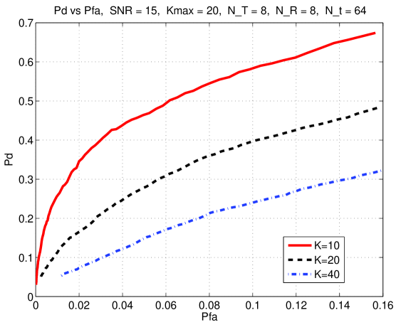
Figure 1: Probability of detection vs. probability of false alarm for SNR = 15 dB, and three values of $K$: $K_{\max}/2,K_{\max},2K_{\max}$.

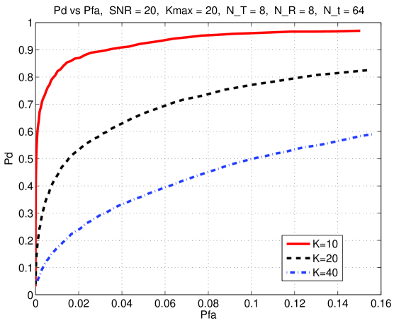
Figure 2: Probability of detection vs. probability of false alarm for SNR = 20 dB, and three values of $K$: $K_{\max}/2,K_{\max},2K_{\max}$.

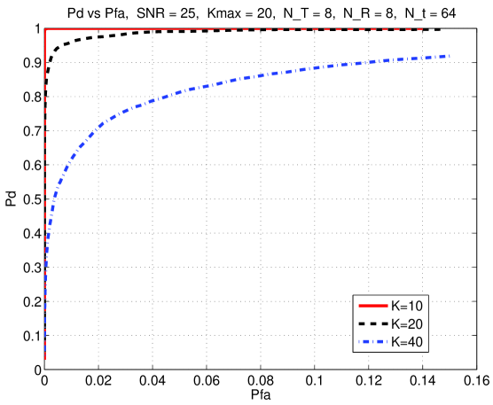
Figure 3: Probability of detection vs. probability of false alarm for SNR = 25 dB, and three values of $K$: $K_{\max}/2,K_{\max},2K_{\max}$.

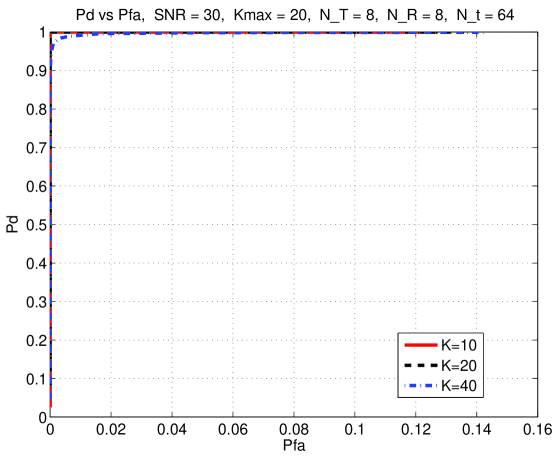
Figure 4: Probability of detection vs. probability of false alarm for SNR = 30 dB, and three values of $K$: $K_{\max}/2,K_{\max},2K_{\max}$.

6 Conclusion

Techniques from compressive sensing and sparse approximation make it possible to exploit the sparseness of radar scenes to potentially improve system performance of MIMO radar. In this paper we have derived a mathematical framework that yields explicit conditions for the radar waveforms and the transmit and receive arrays so that the radar sensing matrix has small coherence and robust sparse recovery in the presence of noise becomes possible. Our approach relies on a deterministic (and very specific) positioning of transmit and receive antennas and random waveforms. It seems plausible that results similar to the ones derived in this paper can be established for the case where the antenna locations are chosen at random and the transmission signals are deterministic. This would be of interest, since one could then potentially take advantage of specific properties of recently designed deterministic radar waveforms such as in [2, 19].

Appendix A

In this appendix we collect some auxiliary results.

Lemma 9

[29, Proposition 34] Let ${\bf x}\in{\mathbb{C}}^{n}$ be a vector with $x_{k}\sim{\cal CN}(0,\sigma^{2})$, then for every $t>0$ one has

$${\mathbb{P}}\Big{(}\|{\bf x}\|_{2}-{\mathbb{E}}\|{\bf x}\|_{2}>t\Big{)}\leq e^{-\frac{t^{2}}{2\sigma^{2}}}.$$ (72)

The following lemma, which relates moments and tails, can be found e.g. in [22, Proposition 6.5].

Lemma 10

Suppose $Z$ is a random variable satisfying

$$({\mathbb{E}}|Z|^{p})^{1/p}\leq\alpha\beta^{1/p}p^{1/\gamma}\qquad\text{for all $p\geq p_{0}$}$$

for some constants $\alpha,\beta,\gamma,p_{0}>0$. Then

$${\mathbb{P}}(|Z|\geq e^{1/\gamma}\alpha u)\leq\beta e^{-u^{\gamma}/\gamma}$$

for all $u\geq p_{0}^{1/\gamma}$.

The following lemma is a rescaled version of Lemma 3.1 in [23].

Lemma 11

Let ${\bf A}\in{\mathbb{C}}^{n\times m}$ be a Gaussian random matrix with $A_{i,j}\sim{\cal CN}(0,\sigma^{2})$. Then for all ${\bf x},{\bf y}\in{\mathbb{C}}^{m}$ with $\|{\bf x}\|_{2}=\|{\bf y}\|_{2}=\sqrt{m}$ and all $t>0$

$${\mathbb{P}}\Big{\{}|\frac{1}{n\sigma^{2}}\langle{\bf A}{\bf x},{\bf A}{\bf y}\rangle-\langle{\bf x},{\bf y}\rangle|>tm\Big{\}}\leq 2\exp\Big{(}-n\frac{t^{2}}{C_{1}+C_{2}t}\Big{)},$$

with $C_{1}=\frac{4e}{\sqrt{6\pi}}$ and $C_{2}=\sqrt{8}e$.

The next lemma is a slight generalization of a result by Hanson and Wright on tail bounds for quadratic forms [12].

Lemma 12

Let ${\bf M}=\{m_{ij}\}_{i,j=1}^{n}$ be a normal matrix and let $X_{i},i=0,\dots,n-1$ be independent, ${\cal CN}(0,1)$-distributed random variables. Denote

$$S_{n}=\sum_{i,j=0}^{n-1}m_{ij}X_{i}\bar{X}_{j}.$$

Then for all $t>0$

$${\mathbb{P}}\Big{(}S_{n}\geq t+{\mathbb{E}}S_{n}\Big{)}\leq\exp\big{(}-C\min\{\frac{t}{\sigma\|{\bf M}\|_{{\text{op}}}},\frac{t^{2}}{\sigma^{2}\|{\bf M}\|_{F}^{2}}\}\big{)},$$

where $C$ is a numerical constant independent of ${\bf M}$ and $n$.

Proof: The proof follows essentially the same steps as the proof of the main theorem in [12], which considers the case where ${\bf M}$ is hermitian and the $x_{i}$ are real-valued. Extending the $x_{i}$ to the complex case is trivial, thus the only modification that needs to be addressed is the extension of ${\bf M}$ from the hermitian to the normal case. But Lemma 5 in [12] holds for normal matrices as well, therefore the lemma follows.  x       

For convenience we state the following version of Bernstein’s inequality, which will be used in the proof of Lemma 14.

Theorem 13 (See e.g. [27])

Let $X_{1},\dots,X_{n}$ be independent random variables with zero mean such that

$${\mathbb{E}}|X_{i}|^{p}\leq\frac{1}{2}p!K^{p-2}v_{i},\qquad\text{for all $i=1,\dots,n;p\in{\mathbb{N}},p\geq 2$},$$

for some constants $K>0$ and $v_{i}>0,i=1,\dots,n$. Then, for all $t>0$

$${\mathbb{P}}\Big{(}\big{|}\sum_{i=1}^{n}X_{i}|\geq t\big{)}\leq 2\exp\Big{(}-\frac{t^{2}}{2v+Kt}\Big{)},$$ (73)

where $v:=\sum_{i=1}^{n}v_{i}$.

We also need the following deviation inequality for unbounded random variables. It is a complex-valued and slightly sharpened version of Lemma 6 in [13], the better constant will be useful when we apply Lemma 14 in the proof of Lemma 3.

Lemma 14

Let $X_{i}$ and $Y_{i}$, $i=1,\dots,n$, be sequences of i.i.d. complex Gaussian random variables with variance $\sigma$. Then,

$${\mathbb{P}}\Big{(}\big{|}\sum_{i=1}^{n}\bar{X}_{i}Y_{i}\big{|}>t\Big{)}\leq 2\exp\big{(}-\frac{t^{2}}{\sigma^{2}(n\sigma^{2}+2t)}\big{)}.$$ (74)

Proof: In order to apply Bernstein’s inequality, we need to compute the moments ${\mathbb{E}}|X_{i}Y_{i}|^{p}$. Since $X_{i}$ and $Y_{i}$ are independent, there holds

$${\mathbb{E}}(|X_{i}Y_{i}|^{p})={\mathbb{E}}(|X_{i}|^{p}){\mathbb{E}}(|Y_{i}|^{p})=({\mathbb{E}}(|X_{i}|^{p}))^{2}.$$

The moments of $X_{i}$ are well-known:

$${\mathbb{E}}|X_{i}|^{2p}=p!\,\sigma^{2p},$$

hence

$$({\mathbb{E}}|X_{i}|^{2p})^{2}=(2p!)^{2}(\sigma^{2p})^{2}\leq\frac{1}{4}(2p)!(\sigma^{2})^{2p}\leq\frac{1}{2}(2p)!(\sigma^{2})^{2p-2}\frac{(\sigma^{2})^{2}}{2}.$$

We apply Bernstein’s inequality (73) with $K=\sigma^{2}$ and $v_{i}=\frac{(\sigma^{2})^{2}}{2},i=1,\dots,n$ and obtain (74).  x       

Appendix B

We consider a general linear system of equations ${\bf\Psi}{\bf x}={\bf y}$, where ${\bf\Psi}\in{\mathbb{C}}^{n\times m}$, ${\bf x}\in{\mathbb{C}}^{m}$ and $n\leq m$. We introduce the following generic $K$-sparse model:

• The support $I\subset\{1,\dots,m\}$ of the $K$ nonzero coefficients of ${\bf x}$ is selected uniformly at random.

• The non-zero entries of $\operatorname{sgn}({\bf x})$ form a Steinhaus sequence, i.e., $\operatorname{sgn}({\bf x}_{k}):={\bf x}_{k}/|{\bf x}_{k}|,k\in I,$ is a complex random variable that is uniformly distributed on the unit circle.

The following theorem is a slightly extended version of Theorem 1.3 in [3].

Theorem 15

Given ${\bf y}={\bf\Psi}{\bf x}+{\bf w}$, where ${\bf\Psi}$ has all unit-$\ell_{2}$-norm columns, ${\bf x}$ is drawn from the generic $K$-sparse model and ${\bf w}_{i}\sim{\cal CN}(0,\sigma^{2})$. Assume that

$$\mu({\bf\Psi})\leq\frac{C_{0}}{\log m},$$ (75)

where $C_{0}>0$ is a constant independent of $n,m$. Furthermore, suppose

$$K\leq\frac{c_{0}m}{\|{\bf\Psi}\|_{{\text{op}}}^{2}\log m}$$ (76)

for some constant $c_{0}>0$ and that

$$\underset{k\in I}{\min}\,|{\bf x}_{k}|>8\sigma\sqrt{2\log m}.$$ (77)

Then the solution $\hat{{\bf x}}$ to the debiased lasso computed with $\lambda=2\sigma\sqrt{2\log m}$ obeys

$$\operatorname{supp}(\hat{{\bf x}})=\operatorname{supp}({\bf x}),$$ (78)

and

$$\frac{\|\hat{{\bf x}}-{\bf x}\|_{2}}{\|{\bf x}\|_{2}}\leq\frac{\sigma\sqrt{3n}}{\|{\bf y}\|_{2}}$$ (79)

with probability at least

$$1-2m^{-1}(2\pi\log m+Km^{-1})-{\cal O}(m^{-2\log 2}).$$ (80)

Proof: The paper [3] treats only the real-values case. However it is not difficult to see that the results by Candès and Plan can be extended to the complex setting if their definition of the sign-function is replaced by (9) and consequently their generic sparse model is replaced by the generic sparsity model introduced in the beginning of this appendix. The proofs of the theorems in [3] can then be easily adapted to the complex case via some straightforward modifications, such as replacing in many steps $\langle\cdot,\cdot\rangle$ by its real part, $\operatorname{Re}\langle\cdot,\cdot\rangle$ and replacing certain scalar quantities by its conjugate analogs. To give a concrete example of such a modification, consider (in the notation of [3]) the inequality right before eq.(3.10) in [3],

$$|\hat{\beta}_{i}|=|\beta_{i}+h_{i}|\geq|\beta_{i}|+\operatorname{sgn}(\beta_{i})h_{i}.$$

This inequality needs to be replaced by its complex counterpart

$$|\hat{\beta}_{i}|=|\beta_{i}+h_{i}|\geq|\beta_{i}|+\operatorname{Re}(\operatorname{sgn}(\beta_{i})\overline{h_{i}}).$$

By carrying out these easy modifications (the details of which are left to the reader) we can readily establish (78) analogous to (1.11) of Theorem 1.3 in [3].

Once we have recovered the support of ${\bf x}$, call it $I$, we can solve for the coefficients of ${\bf x}$ by solving the standard least squares problem $\min\|{\bf A}_{I}{\bf x}_{I}-{\bf y}\|_{2}$, where ${\bf A}_{I}$ is tbe submatrix of ${\bf A}$ whose columns correspond to the support set $I$, and similarly for ${\bf x}_{I}$. Statement (79) follows by noting that the proof of Theorem 3.2 in [3] yields as side result that with high probability the eigenvalues of any submatrix ${\bf A}_{I}^{\ast}{\bf A}_{I}$ with $|I|\leq K$ are contained in the interval $[1/2,3/2]$, which of course implies that $\kappa({\bf A}_{I})\leq\sqrt{3}$. The statement follows now by substituting this bound into the standard error bound, eq. (5.8.11) in [17].  x

References

• [1] S. Becker, E. Candès, and M. Grant. Templates for convex cone problems with applications to sparse signal recovery. Mathematical Programming Computation 3(3), 165–218, 2011.
• [2] J.J. Benedetto and S. Datta. Construction of infinite unimodular sequences with zero auto correlation. Advances in Computational Mathematics, 32:191–207, 2010.
• [3] E.J. Candès and Y. Plan. Near-ideal model selection by $\ell_{1}$ minimization. Annals of Statistics, 37(5A):2145–2177, 2009.
• [4] E.J. Candès and T. Tao. Near-optimal signal recovery from random projections: Universal encoding strategies. IEEE Trans. on Information Theory, 52:5406–5425, 2006.
• [5] E.J. Cand$\grave{\text{e}}$s and Y. Plan. A Probabilistic and RIPless Theory of Compressed Sensing. IEEE Transactions on Information Theory, 57(11):7235–7254, 2011.
• [6] M. Cheney and B. Borden. Fundamentals of Radar Imaging. Society for Industrial and Applied Mathematics, 2009.
• [7] Y. Chi, A. Pezeshki, L. Scharf, and R. Calderbank. Sensitivity to basis mismatch in compressed sensing. IEEE Trans. Signal Processing, 59(5): 2182-2195, 2011.
• [8] D. L. Donoho. Compressed sensing. IEEE Trans. on Information Theory, 52(4):1289–1306, 2006.
• [9] A. Fannjiang and W. Liao. Coherence pattern–-guided compressive sensing with unresolved grids. SIAM J. Imaging Sci., 5:179–202, 2012.
• [10] B. Friedlander. Adaptive Signal Design for MIMO Radar. In J. Li and P. Stoica, editors, MIMO Radar Signal Processing, chapter 5. John Wiley & Sons, 2009.
• [11] B. Friedlander. On the relationship between MIMO and SIMO radars. IEEE Trans. Signal Processing, 57(1):394–398, January 2009.
• [12] D.L. Hanson and F.T. Wright. A bound on tail probabilities for quadratic forms in independent random variables. The Annals of Mathematical Statistics, 42(3):1079–1083, 1971.
• [13] J. Haupt, W. Bajwa, G. Raz, and R. Nowak. Toeplitz compressed sensing matrices with applications to sparse channel estimation. IEEE Trans. Inform. Theory, 56(11):5862–5875, 2010.
• [14] C. Helstrom. Elements of Signal Detection and Estimation. Prentice Hall, 1995, 2005.
• [15] M. Herman and T. Strohmer. High-resolution radar via compressed sensing. IEEE Trans. on Signal Processing, 57(6):2275–2284, 2009.
• [16] M. Herman and T. Strohmer. General deviants: an analysis of perturbations in compressed sensing. IEEE Journal of Selected Topics in Signal Processing: Special Issue on Compressive Sensing, 4(2):342–349, 2010.
• [17] R.A. Horn and C.R. Johnson. Matrix analysis. Cambridge University Press, Cambridge, 1990. Corrected reprint of the 1985 original.
• [18] J. Li and P. Stoica, editors. MIMO Radar Signal Processing. John Wiley & Sons, 2009.
• [19] A. Pezeshki, A.R. Calderbank, W. Moran, and S.D. Howard. Doppler resilient Golay complementary waveforms. IEEE Transactions on Information Theory, 54(9):4254–4266, 2008.
• [20] G.E. Pfander, H. Rauhut, and J. Tanner. Identification of matrices having a sparse representation. IEEE Trans. Signal Processing, 56(11):5376–5388, 2008.
• [21] L. C. Potter, E. Ertin, J. T. Parker, and M. Cetin. Sparsity and compressed sensing in radar imaging. Proceedings of the IEEE, 98(6):1006 –1020, 2010.
• [22] H. Rauhut. Compressive sensing and structured random matrices. In Theoretical Foundations and Numerical Methods for Sparse Recovery, volume 9 of Radon Series Comp. Appl. Math., pages 1–92. deGruyter, 2010.
• [23] H. Rauhut, K. Schnass, and P. Vandergheynst. Compressed sensing and redundant dictionaries. IEEE Transactions on Information Theory, 54(5):2210–2219, 2008.
• [24] A. W. Rihaczek. High-Resolution Radar. Artech House, Boston, 1996. (originally published: McGraw-Hill, NY, 1969).
• [25] L.L. Scharf. Statistical Signal Processing. Prentice Hall, 1990.
• [26] R. Tibshirani. Regression shrinkage and selection via the lasso. J. Roy. Statist. Soc. Ser. B, 58(1):267–288, 1996.
• [27] A.W. van der Vaart and J.A. Wellner. Weak convergence and empirical processes. Springer Series in Statistics. Springer-Verlag, New York, 1996. With applications to statistics.
• [28] H.L. Van Trees. Detection, Estimation, and Modulation Theory, Part I. Wiley-Interscience, 2001.
• [29] R. Vershynin. Introduction to the non-asymptotic analysis of random matrices. In Yonina C. Eldar and Gitta Kutyniok, editors, Compressed Sensing: Theory and Applications. Cambridge University Press, 2010. To Appear. Preprint available at http://www-personal.umich.edu/~romanv/papers/papers.html.
• [30] Y. Yu, A. Petropulu, and V. Poor. Measurement matrix design for compressive sensing-based MIMO radar. IEEE Trans. on Signal Processing, 59(11):5338–5352, 2011.
• [31] Y. Yu, A. Petropulu, and V. Poor. CSSF MIMO RADAR: Low-complexity compressive sensing based MIMO radar that uses step frequency. IEEE Trans. on Aerospace and Electronic Systems, to appear.