Modifying the HF procedure to include screening effects

Abstract

A self-consistent formulation is proposed to generalize the HF scheme with the incorporation of screening effects. For this purpose in a first step, an energy functional is defined by the mean value for the full Hamiltonian, not in a Slater determinant state, but in the result of the adiabatic connection of Coulomb plus the nuclear (jellium charge) in the Slater determinant. Afterwards, the energy functional defining the screening approximation is defined in a diagrammatic way, by imposing a special ”screening” restriction on the contractions retained in the Wick expansion. The generalized self-consisting set of equations for the one particle orbitals are written by imposing the extremum conditions. The scheme is applied to the homogeneous electron gas. After simplifying the discussion by assuming the screening as static and that the mean distance between electrons is close to the Bohr radius, the equations for the electron spectrum and the static screening properties are solved by iterations. The self-consistent results for the self-energies dispersion does not show the vanishing density of states at the Fermi level predicted by the HF self-energy spectrum. In this extreme non retarded approximation, both, the direct and the exchange potentials are strongly screened, and the energy is higher that the one given by the usual HF scheme. However, the inclusion of the retardation in the exact solution and the sum rules associated to the dielectric response of the problem, can lead to energy lowering. These effects will be considered in the extension of the work.

I Introduction

The development of band structure calculation procedures is a theme to which an intense research activity has been devoted in modern Solid State Physics. This area of research has a long history due to existence of important unsolved and relevant questions concerning the structure of solids mott1 ; slater1 ; slater ; bmuller ; dagoto ; almasan ; yanase ; vanharlingen ; damascelli ; pickett ; Burns ; imada ; freltoft ; deBoer ; peierls ; anderson1 ; hubbard ; adersson ; fradkin ; gutzwiller ; gutzwiller1 ; rice ; kohn ; kohn1 ; terakura ; singh ; szabo ; fetter ; matheiss ; mott . One central open problem is the connection between the so called first principles schemes with the Mott phenomenological approach. This important approach, furnishing the descriptions for a wide class of band structures of solids, is not naturally explained by the assumed fundamental first principles approaches mott ; slater ; imada ; yanase ; dagoto . A class of materials which had been in the central place in the existing debate between these two conceptions for band structure calculations are the transition metal oxides (TMO) pickett ; imada ; yanase ; anderson1 ; terakura ; hubbard ; gutzwiller ; gutzwiller1 . A particular compound which is closely related with the TMO is the superconductor material $La_{2}CuO_{4}$ in which the first band structure calculations predicted metal and paramagnetic characters, which are largely at variance with the known isolator and antiferromagnetic nature of the material matheiss . Actually, these two qualities are fully believed to be purely strong correlation properties which are not derivable from HF independent particle descriptions anderson1 ; terakura ; augustoref . However, in Refs. pla ; symmetry a single band Hartree-Fock (HF) study was able to produce these assumed strong correlation properties of $La_{2}CuO_{4}$, as independent particle ones, arising from a combination of crystal symmetry breaking in and an entanglement of the spin and spacial structure of the single particle states. Therefore, this result opens the interesting possibility of clarifying the connection between the Mott and Slater viewpoints in the band theory of the TMO pla ; symmetry . It should be underlined that a former HF study of $La_{2}CuO_{4}$ in Ref. su , also indicated an insulator an AF character of the material. However, the extremely large gap ( $17$ eV) which was predicted by that work had a radical discrepancy with the experimentally estimated value of $2$ eV. However, it could happens that the results of Ref. su could show a close link with the conclusions of Refs. pla ; symmetry . Results in the literature supporting this possibility are the ones presented in Ref. perry , where the same recourse employed in Refs. pla ; symmetry of allowing a crystal symmetry breaking by doubling the unit cell of the lattice was employed. In that work, the spin was treated in a phenomenological way by including a spin dependent functional in the variational evaluation done. These two procedures allowed the authors to predict an insulator and AF structure for the material with a gap of 2 $eV$, well matching the experimental estimate.

The results in Ref. pla ; symmetry were obtained  by starting form a Tight Binding (T.B.) model with a square lattice size equal to the distance between Cu atoms in the CuO planes, by assuming a simple crystalline extended quadratic (near the Cu atoms) T.B. potential. The strength of the potential was fixed to reduce the width of the states to be smaller than the chosen lattice constant to obey the T.B. condition.  Afterwards the metal paramagnetic HF bands obtained when considering the Coulomb interaction in the model,  was fixed to approximately reproduce the single half filled band crossing the Fermi level, obtained in the evaluation of the band structure of $La_{2}CuO_{4}$ in Ref. matheiss .  A curious point was that the value of the dielectric constant that was required to make equal the two bandwidths  was nearly $\epsilon=10$ . Therefore, it come to the mind that the introduction of a dielectric constant in the HF equations of Ref. su , might be produced a band gap of nearly $1.7$  eV for $La_{2}CuO_{4},$ being very close to the measured one of $2$ eV.  This indicates that if a HF method could be extended to predict the screening properties, it could has the chance of  explaining the strongly correlation properties of $La_{2}CuO_{4}$ and with luck, of its close related parents, the transition metal oxides.  The possibility exist that such an approach could furnish a simple way of catching the strong correlation properties of these materials giving in this way a clear explanation for the Mott properties, by showing its connection with the crystal symmetry breaking and spin-space entangled nature of single particle states pla ; symmetry .

Therefore, in this paper we intend to start generalizing the HF scheme to introduce screening effects. A first possibility is considered here by constructing an energy functional $E$ to be optimized by a set of single particle states. The functional $E$ for the HF scheme is simply taken as the mean value of the exact Hamiltonian in the Slater determinant of formed by the single particle functions over which $E$ is optimized.

Since we are interested in introducing Coulomb interaction effects, a first general possibility consists in modifying the variational Slater determinant of the single particle functions by connecting in it the Coulomb interaction between the electrons and with nuclear ”jellium” potential by employing the Gell-Mann-Low procedure gellmann ; goldstone ; thouless ; fetter .̇ This definition will have variational character, that is, will be equal to a mean value of the total Hamiltonian in one state, and thus the result after finding the extremes over the one particle states, should be greater than the ground state energy of the system.  However, the complications in solving the extremum equations following from introducing the Coulomb and nuclear interaction in an exact form will be enormous.  However, we are only interested in catching improvement on the HF scheme produced by more simple screening processes. Then, it becomes possible to approximate the above mentioned state (the one resulting of the connection of the electronic interactions) by restricting the sum over all the Feynman graphs to a set reflecting screening properties. Then, the simpler state will be chosen by only retaining in the sum given by the Wick expansion, only the graphs for which: a) for any line arriving to a point of a vertex and coming from a another different point, always exists another different line that joins the same two points.  This definition basically retains the diagrams in which are essentially the ”tree” diagrams (having now closed loops) in which arbitrary number of insertions of the polarization loop are included. The functional $E$ defined as the mean value of the Hamiltonian is also an upper bound for the ground state energy. However, this functional expression although simpler, yet will  lead to slightly cumbersome procedure. Thus, we defer its study to eventual future discussion.  In order to further simplify the form of the functional, but yet retaining screening effects, we even more simplify the functional by imposing the same screening approximation to the whole sum of Feynman diagrams which defines the functional $E$ in which the Coulomb and nuclear interactions are adiabatically connected.  This definition leads to scheme which is formulated in very close terms with the usual discussions of the screening approximation in Many Body theory kadanoff .

Up to now, we had not been able to show that this approximation also has a variational character. However, at least it follows that the Feynman diagrams  defining the scheme represent allowed physical process, which suggests that the procedure can improve the HF results.  If the variational character turns to be valid, the result for energy will also furnish an upper bound for the ground state energy. This issue will be considered elsewhere.

After defining $E$, the generalized HF equations are derived for the general case of inhomogeneous electron systems. They include exchange and direct like terms, but also show additional contributions being related with effect of the Coulomb interaction and nuclear potential on the kinetic energy of the electron which vanish for homogeneous systems. The equations are also written for the case homogeneous electron gas in which the full translation symmetry simplifies them. In this case, as in the usual HF scheme, only the kinetic and exchange terms are non vanishing. In this first exploration, it is assumed that the screening is static and the density is chosen to be one electron per sphere of radial dimension equal to the Bohr radius. Under these conditions, the self-consistent equations for the electron spectrum and the static screening properties are solved by iterations. The result for the dispersion does not present the vanishing density of states at the Fermi energy appearing in the fist in the HF self-energy spectrum kittel ; madelung ; raimes ; callaway ; zerodensity .

The work proceeds as follows. In Section II, the generalization of the HF functional and equations of motions for the single particle orbitals are presented. Section III then considers the application to the homogenous electron gas. In the conclusions the results are reviewed and possible extensions of the work are commented.

II Generalization of the HF scheme to include screening effects

II.1 Hartree Fock approximation

As it is known the HF approximation is obtained after minimizing the mean value of the full Hamiltonian of the system $H$ in a Slater determinant state $\ |\!$ $\Phi_{0}\rangle$  formed with the elements of a basis of wavefunctions $\varphi_{k}$.  For future purposes, let us define a free Hamiltonian $H_{0}$ in terms for these functions in the form

$$H_{0}=\sum_{k}\epsilon_{k}\text{ }a_{k}^{+}a_{k},$$ (1)

where $a_{k}^{+}$ and $a_{k}$ are the creation and annihilation operators of the functions $\varphi_{k}(\mathbf{x})$ and the energy eigenstates $\{\epsilon_{k}\}$ are to be defined by the optimization process of the energy functional

$$E[\varphi] =\ \langle\!\Phi_{0}|\text{ }H\ |\!\Phi_{0}\rangle-{\displaystyle\sum\limits_{kl}}\lambda_{kl}(\int d\mathbf{x}\text{ }\varphi_{k}^{\ast}(\mathbf{x})\varphi_{l}(\mathbf{x})-\delta_{kl}),$$ (2)

$$\langle\mathbf{x}_{1},\mathbf{x}_{2},...{\small,}\mathbf{x}_{N_{p}}|\!\Phi_{0}\rangle =\frac{1}{N_{p}!}Det\text{ }[\varphi_{k}(\mathbf{x}_{l})]$$ (3)

where $N_{p}$ is the number of electrons.  The bold letters will represent the combination of the position $\overrightarrow{x}$ and spin $s=\pm 1$ coordinates as $\mathbf{x}=(\overrightarrow{x},s)$ and the integrals will mean

$$\int d\mathbf{x=}{\displaystyle\sum\limits_{s=\pm 1}}\int d\text{ }\overrightarrow{x}.$$

In addition, in order to simplify the expressions when time dependence will be considered we will define also space-time coordinates $x=(\mathbf{x},t)=(\overrightarrow{x},s,t).$

The system to be considered will be a set of electrons which move in the presence of a nuclear potential $V_{nuc}$ and interact among themselves with the Coulomb two body potential $v$.  After adding the kinetic energy $T$ of the electrons, the total Hamiltonian is given in the Schrodinger coordinate representation as

$$H =T+V_{nuc}+v,$$ (4)

$$T \equiv-\sum_{i=1}^{N_{p}}\frac{\hslash^{2}}{2m}\partial_{i}^{2},\text{ \ \ \ }\partial_{i}=\frac{\partial}{\partial\text{ }\overrightarrow{x}_{i}},$$ (5)

$$V_{nuc} \equiv-\sum_{i=1}^{N_{p}}\int d\text{ }\overrightarrow{z}\text{ }\rho_{nuc}(\overrightarrow{z})\frac{e^{2}}{|\overrightarrow{z}-\overrightarrow{x}_{i}|},$$ (6)

$$v \equiv\sum_{\begin{subarray}{c}i,j=1\\ i\neq j\end{subarray}}^{N_{p}}\frac{1}{2}\frac{e^{2}}{|\overrightarrow{x}_{i}-\overrightarrow{x}_{j}|},$$ (7)

and, in what follows, in order to simplify the notation, all the operators acting in coordinate space appearing, will be supposed to have a spin structure, which when not written,  are assumed to be the identity matrix in the representation of the functions on which the operators act.  Imposing the extremum conditions on $E$ over the variations of the functions, the $HF$ equations for determining the single particle states follow.  The fact that, on the extremum values of the single particle functions, it is satisfied   the $E=\langle\!\Phi_{0}|$ $H\ |\!\Phi_{0}\rangle,$ implies

$$E\geq E_{g},$$ (8)

where $E_{g}$ is the ground state energy, which for a Hamiltonian system gives the lowest mean value possible in any state.

Let us now intend to construct a generalization of the $HF$ method including screening effects.  For this purpose, initially, let us define the functional to be optimized in an alternative form assuring that the result includes Coulomb interaction effects. A possible form of this kind is the following one

$$E =\ \frac{\langle\!\Phi_{0}|(U_{\alpha}^{c\text{ }}(0,-\infty))^{+}H\text{ }U_{\alpha}^{c}(0,-\infty)\ |\!\Phi_{0}\rangle}{\langle\!\Phi_{0}|(U_{\alpha}^{c\text{ }}(0,-\infty))^{+}U_{\alpha}^{c}(0,-\infty)\ |\!\Phi_{0}\rangle}$$

$$=\frac{\langle\!\Phi_{0}|U_{\alpha}^{c\text{ }}(\infty,0)\text{ }H\text{ }U_{\alpha}^{c}(0,-\infty)\ |\!\Phi_{0}\rangle}{\langle\!\Phi_{0}|U_{\alpha}^{c\text{ }}(\infty,0)U_{\alpha}^{c}(0,-\infty)\ |\!\Phi_{0}\rangle},$$ (9)

in which $U_{\alpha}^{c}$ is the evolution operator connecting the Coulomb interaction among the electrons plus the nuclear potential $V_{nuc}+v,$ in an initial previously defined Slater determinant $|\,\Phi_{0}\rangle$ (the ground state of the free Hamiltonian $H_{0})$ at a large time in the past

$$U_{\alpha}^{c}(0,-\infty) =\sum_{n=0}^{\infty}\frac{(\frac{-i}{\hslash})^{n}}{n!}\int_{-\infty}^{0}dt_{1}\int_{-\infty}^{0}dt_{2}...\int_{-\infty}^{0}dt_{n}\text{ }T\text{ }[H_{\alpha}^{c}(t_{1}),H_{\alpha}^{c}(t_{2}),H_{\alpha}^{c}(t_{3})...,H_{\alpha}^{c}(t_{n})],$$

$$=T\text{ }[\exp(-\frac{i}{\hslash}\int_{-\infty}^{0}dt\text{ }H_{\alpha}^{c}(t))],$$ (10)

$$H_{\alpha}^{c}(t) =\exp(\frac{i}{\hbar}H_{0}t)\text{ }H^{c}\exp(-\frac{i}{\hbar}H_{0}t)\text{ }{\large e}^{(-\alpha\text{ }|\text{ }t\text{ }|)},$$ (11)

$$H^{c} =V_{nuc}+v,$$ (12)

where $H^{c}$ is the sum of the Coulomb and nuclear electron interactions in a time independent Schrodinger representation, $\alpha$ is the Gell-Mann-Low small parameter which implements the adiabatic connection of the interaction when taken in the limit $\alpha\rightarrow 0^{+}.$ The $\alpha$   dependent exponential factor appearing in the definition of the interaction representation operators $H_{\alpha}^{c}(t)$ above, tends to one when $\alpha$ vanishes gellmann ; goldstone ; fetter .  The $T$ symbol appearing is the time ordering operation which orders the operators from right to left for increasing  time arguments gellmann ; goldstone ; fetter .

For the Hermitian conjugate operator $U_{\alpha}^{c+}$ it follows

$$(U_{\alpha}^{c}(0,-\infty))^{+} =\sum_{n=0}^{\infty}\frac{(\frac{i}{\hslash})^{n}}{n!}\int_{-\infty}^{0}dt_{1}\int_{-\infty}^{0}dt_{2}...\int_{-\infty}^{0}dt_{n}\text{ }T^{\ast}\text{ }[H_{\alpha}^{c}(t_{1}),H_{\alpha}^{c}(t_{2}),H_{\alpha}^{c}(t_{3})...,H_{\alpha}^{c}(t_{n})],$$

$$=.T^{\ast}\text{ }[\exp(\frac{i}{\hslash}\int_{-\infty}^{0}dt\text{ }H_{\alpha}^{c}(t))]$$

$$=T\text{ }[\exp(\frac{i}{\hslash}\int_{\infty}^{0}dt^{\ast}H_{\alpha}^{c}(t^{\ast}))]=T\text{ }[\exp(-\frac{i}{\hslash}\int_{0}^{\infty}dt^{\ast}H_{\alpha}^{c}(t^{\ast}))]$$

$$=U_{\alpha}^{c}(\infty,0).$$ (13)

Noticing that $H$ is equal to its interaction representation $H(t)=\exp(\frac{i}{\hbar}H_{0}t)$ $H\exp(-\frac{i}{\hbar}H_{0}t)$ ${\large e}^{(-\alpha\text{ }|\text{ }t\text{ }|)}$ at $t=0$

$$H(0)=T(0)+V_{nuc}(0)+v(0),$$ (14)

it follows that in formula (9), the operators are temporally ordered. Therefore, the Wick theorem can be applied.  The sum of the expressions associated to all the Feynman diagrams giving the denominator, coincides with the sum of all the possible terms associated to disconnected (unlinked) graphs of the numerator, multiplying the contribution of a given arbitrary connected graph.  Thus, this common factor cancels gellmann ; goldstone ; fetter .  The expression for $E$ in this general form is given by the sum of the contributions being associated to all the diagrams being connected through their vertices and lines to the vertices defined by the operator $H.$ In this case, since $E$ is again a mean value of $H$ in a given state, it follows that $E$ should be greater than the ground state energy $E_{g}$

In spite of this property, the complexity of the sum over all the connected part will surely make the optimization problem an impossible to be solved one.  Thus, it is needed to further simplifying the functional incorporating

the screening effects.

II.2 Screening approximation

As it was just mentioned, the general form of the variational problem defined by (9) is too complicated for to be usable in concrete evaluations. Let us consider in this section two simplifications. They will be called as ”screening” ones, and will be implemented through an approximation of the Wick theorem. In the Wick expansion, the time ordered products of creation and annihilation operators are expressed as the sum of all normally ordered products including an arbitrary number of contractions between any pair of operators entering in the product. The terms in this expansion are related by a one-to-one mapping with all the diagrams generated by the Feynman rules of the theory gellmann ; goldstone ; fetter .

The first ”screening” approximation to be considered will be one in which a variational state $|\,\Phi_{s}\rangle=U_{\alpha}^{(s)}\ |\,\Phi_{0}\rangle$ is defined after applying the Wick expansion to the operator $U_{\alpha}^{c}(0,-\infty)$ entering in the definition of the state $U_{\alpha}^{c}(0,-\infty)\ |\!\Phi_{0}\rangle.$ In the Feynman diagram expansion of the operator only the graphs will retained in which,  for any particular line joining two different ending points of any vertices, another different line always exists connecting the same two points goldstone .  We will describe this reduction of the diagrams associated to a time ordered operators $A$ by writing $[A]_{WS}$. Then, the variational state $|\,\Phi_{s}\rangle$ will have the form

$$U_{\alpha}^{(s)}|\!\Phi_{0}\rangle =\left[U_{\alpha}^{c}(0,-\infty)\right]_{WS}|\!\Phi_{0}\rangle$$

$$=\sum_{n=0}^{\infty}\frac{(\frac{-i}{\hslash})^{n}}{n!}\int_{-\infty}^{0}dt_{1}\int_{-\infty}^{0}dt_{2}...\int_{-\infty}^{0}dt_{n}\text{ }{\large[}T\text{ }[H_{\alpha}^{c}(t_{1}),H_{\alpha}^{c}(t_{2}),H_{\alpha}^{c}(t_{3})...,H_{\alpha}^{c}(t_{n})]{\large]}_{WS}|\!\Phi_{0}\rangle$$ (15)

and its Hermitian conjugate state satisfies

$$\langle\Phi_{0}|U_{\alpha}^{(s)} =\left[\langle\Phi_{0}|U_{\alpha}^{c}(\infty,0)\ \right]_{WS}$$

$$=\sum_{n=0}^{\infty}\frac{(\frac{-i}{\hslash})^{n}}{n!}\int_{0}^{\infty}dt_{1}\int_{0}^{\infty}dt_{2}...\int_{0}^{\infty}dt_{n}\text{ }\langle\Phi_{0}|\left[T\text{ }[H_{\alpha}^{c}(t_{1}),H_{\alpha}^{c}(t_{2}),H_{\alpha}^{c}(t_{3})...,H_{\alpha}^{c}(t_{n})]\right]_{WS}$$

$$=\langle\Phi_{0}|\left[T\text{ }[\exp(-\frac{i}{\hslash}\int_{0}^{\infty}dt\text{ }H_{\alpha}^{c}(t))]\right]_{WS}.$$ (16)

It is clear that since the $E$ functional is defined as a mean value in the given normalized state, the minimization of $E$ process will be variational, that is $E>Eg.$ Since the criterion for eliminating a contribution is only determined by the contractions between two linked vertices, the application to the screening approximation to a product of two to disconnected graphs $G_{1}$ and $G_{2}$ in which all the operators are contracted, gives the product of the two independently approximated graphs. That is, the same property as for the Wick expansion

$$[G_{1}G_{2}]_{WS}=[G_{1}]_{WS}[G_{2}]_{WS}.$$ (17)

The approximation done in defining the state eliminates all the graphs in the Wick expansion of the state $U_{\alpha}^{c}(0,-\infty)\ |\!\Phi_{0}\rangle.$ But when the scalar product defining $E$  is taken, a new application of the Wick expansion to the full operator $U_{\alpha}^{(s)+}HU_{\alpha}^{(s)}$ leads to diagrams not satisfying the defined screening approximation. That is, diagrams exist for which not all the internal fermion lines appears in polarization loops and tadpoles.  This fact is not an obstacle of principle, but it leads to an structure of the connected to $H$ sum of Feynman diagrams in which somewhat complicated three and four loops diagrams appear.  Then, in this work will not use the approximation in this form.  Rather, in order to retaining contributions consistently being given by diagrams showing the imposed ”screening” graphical restriction, the functional $E$ will be defined in the form

$$E=\frac{\langle\Phi_{0}|[U_{\alpha}^{(c)+}HU_{\alpha}^{(c)}]_{WS}|\!\Phi_{0}\rangle}{\langle\Phi_{0}|[U_{\alpha}^{(c)+}U_{\alpha}^{(c)}]_{WS}|\!\Phi_{0}\rangle},$$ (18)

in which, the modified Wick expansion $[\,\,\,]_{WS}$ is applied to the whole operators $U_{\alpha}^{(c)+}HU_{\alpha}^{(c)}$ and $U_{\alpha}^{(c)+}U_{\alpha}^{(c)}$.

After expanding the exponential defining the operators, the numerator has the expression

$$\langle\Phi_{0}|[U_{\alpha}^{(c)+}HU_{\alpha}^{(c)}]_{WS}|\!\Phi_{0}\rangle =\sum_{n_{2}=0}^{\infty}\frac{(\frac{-i}{\hslash})^{n_{2}}}{n_{2}!}\int_{0}^{\infty}dt_{1}\int_{0}^{\infty}dt_{2}...\int_{0}^{\infty}dt_{n_{2}}\text{ }$$

$$\sum_{n_{1}=0}^{\infty}\frac{(\frac{-i}{\hslash})^{n_{1}}}{n_{1}!}\int_{-\infty}^{0}dt_{1}^{\prime}\int_{-\infty}^{0}dt_{2}^{\prime}...\int_{-\infty}^{0}dt_{n_{1}}^{\prime}$$

$$\langle\Phi_{0}|{\LARGE[}T\text{ }[H_{\alpha}^{c}(t_{1}),H_{\alpha}^{c}(t_{2}),H_{\alpha}^{c}(t_{3})...,H_{\alpha}^{c}(t_{n_{2}})]\times$$

$$H\times$$

$$T\text{ }[H_{\alpha}^{c}(t_{1}^{\prime}),H_{\alpha}^{c}(t_{2}^{\prime}),H_{\alpha}^{c}(t_{3}^{\prime})...,H_{\alpha}^{c}(t_{n_{1}}^{\prime})]{\LARGE]}_{WS}|\!\Phi_{0}\rangle,$$ (19)

and the denominator has a similar one, obtained by omitting the $H$ operator.

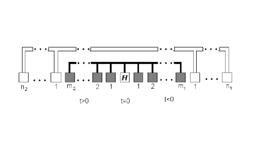
Figure 1: The figure illustrates the terms associated to the product of the power $(n_{1}+m_{1})$ in the series expansion of $U_{\alpha}^{(c)}$ and the power $(n_{2}+m_{2})$ of the expansion of the operator $U_{\alpha}^{(c)+}$ in formula (19) for the $E$ functional.

The figure (1) is a pictorial representation of the terms associated to the product of the power $(n_{1}+m_{1})$ in the series expansion of $U_{\alpha}^{(c)}$ and the power $(n_{2}+m_{2})$ of the expansion of the operator $U_{\alpha}^{(c)+}$ in formula (19) for the $E$ functional. Each square represents one interaction operator $v+V_{nuc}$ evaluated a given time, which grows from right to left in the picture.  The illustrated term represents a particular contribution to the approximated Wick expansion adopted. In it, the white squares represent vertices which have contractions between the operators defining them. Such contractions are in such a form that the graph associated to these vertices and contractions are not connected to the vertices in the operator $H.$ The white channels joining such vertices represent the set of contractions in the illustrated contribution. Alternatively, the black squares represent all the vertices of the interactions $v+V_{nuc}$ being connected among them and with vertices in $H$ by contractions. The square labeled with the letter $H$  represents any of the vertices in the total Hamiltonian. The number $m_{1}$ of black squares come from the expansion of $U_{\alpha}^{(c)}$ and the number $m_{2}$ from the expansion of $U_{\alpha}^{(c)+}.$  The black channels in this case symbolize the set of contractions between operators associated to these vertices.  The fact that all the terms in the Wick expansion are normal orderings including contractions, allows to reorder in the time direction all the square boxes in an arbitrary way. This follows because each vertex has an even number of these operators and the normal ordering are even under a permutations of groups of even numbers of such operators.  Therefore, the same contribution to the result of the expansion will be obtained from the $\frac{(n_{1}+m_{1})!}{n_{1}!}$ terms appearing the expansion of the exponential operator $U_{\alpha}^{(c)},$ each of which has a coefficient$\frac{1}{(n_{1}+m_{1})!}$. In the same way, the $\frac{(n_{1}+m_{1})!}{n_{1}!}$  number of identical contributions in the expansion of $U_{\alpha}^{(c)+}$ changes the original coefficient $\frac{1}{(n_{2}+m_{2})!}$ by  $\frac{1}{n_{2}!}.$ Thus, each connected contribution will be multiplied by the sum of the same contributions defining the denominator $\langle\Phi_{0}|[U_{\alpha}^{(c)+}U_{\alpha}^{(c)}]_{WS}|\!\Phi_{0}\rangle.$ in which $H$ is not appearing. Therefore, the functional $E$ is defined by the sum of all the contributions associated to the Feynman diagrams only including ”screening” contributions being connected to the operator $H$.  It is not ruled out this second type of screening approximation also gives a  value of $E$ being an upper bound for the ground state energy. However, we had yet found a proof of the property, and it will be expected to be considered elsewhere.  In spite of this fact, since the HF approximation furnishes good results for the energy of many systems of interest, leads to the expectation that the inclusion of the screening effect can provide improvements of the HF results for the total energy as well as for the excitation spectrum at least in some situations of physical interest.

II.3 Analytic expression of the functional

Let us write in more detail the Hamiltonian of the system as written in second quantization, and the rules for the Feynman diagrams in the considered general many electron problem. The definition and notation follow the ones in Ref. thouless . The Hamiltonian in second quantization has the form

$$H(t) =T(t)+V_{nuc}(t)+v(t),$$ (20)

$$T(t) \equiv-\int d\text{ }\mathbf{x}\frac{\hslash^{2}}{2m}\Psi^{+}(x)\partial_{i}^{2}\Psi(x),\text{ \ \ \ }\partial_{i}=\frac{\partial}{\partial\overrightarrow{x}_{i}},$$ (21)

$$V_{nuc}(t) \equiv-\int d\text{ }\overrightarrow{z}\text{ }\rho_{nuc}(\overrightarrow{z})\frac{e^{2}}{|\overrightarrow{z}-\overrightarrow{x}|}\int d\text{ }\mathbf{x}\text{ }\Psi^{+}(x)\Psi(x),$$ (22)

$$v(t) \equiv\int d\text{ }x\int d\text{ }x\text{\'{}}\frac{1}{2}\Psi^{+}(\overrightarrow{x}\mathbf{,}s,t)\Psi^{+}(\overrightarrow{x}\acute{},s\acute{},t\text{ }\acute{})\frac{e^{2}\delta(t-t\acute{})}{|\overrightarrow{x}-\overrightarrow{x}\acute{}|}\Psi^{+}(\overrightarrow{x}\acute{},s\acute{},t\text{\'{}})\text{ }\Psi^{+}(\overrightarrow{x}\mathbf{,}s,t),$$ (23)

$$\Psi(x) ={\displaystyle\sum\limits_{k}}a_{k}(t)\text{ }\varphi_{k}(\mathbf{x})={\displaystyle\sum\limits_{k}}a_{k}\exp(-\frac{i}{h}\epsilon_{k}t)\varphi_{k}(\mathbf{x}),$$ (24)

$$\Psi^{+}(x) ={\displaystyle\sum\limits_{k}}a_{k}^{+}(t)\text{ }\varphi_{k}^{\ast}(\mathbf{x})={\displaystyle\sum\limits_{k}}a_{k}^{+}\exp(\frac{i}{h}\epsilon_{k}t)\varphi_{k}^{\ast}(\mathbf{x}),$$ (25)

The above Hamiltonian leads to a diagram expansion as follows. The directed continuous lines represent the free fermion propagator (contractions) associated to the Hamiltonian $H_{0}$

$$G(x,x^{\prime}) =\int\frac{dw}{2\pi}\sum_{k}\frac{i\text{ \ }\varphi_{k}(\mathbf{x})\varphi_{k}^{\ast}(\mathbf{x}^{\prime})\exp(-i\text{ }w(t-t^{\prime}-\delta))}{(w-\frac{1}{\hbar}\epsilon_{k}+i\text{ }\alpha\text{ }sgn(\epsilon_{k}-\epsilon_{f}))}$$

$$=\sum_{k}\varphi_{k}(\mathbf{x})\varphi_{k}^{\ast}(\mathbf{x}^{\prime})(\theta(t-t^{\prime}-\delta)\theta(\epsilon_{k}-\epsilon_{f})-\theta(t^{\prime}-t+\delta)\theta(\epsilon_{f}-\epsilon_{k}),$$

$$\delta \rightarrow 0^{+},$$

where, as defined before, $\alpha$ is the small parameter introduced for connecting the interaction and $\delta$ is small time splitting which is required to well define the time ordering for equal time operators in each interaction Hamiltonian according to the convention in Ref. thouless . In particular it assures the appearance of the usual $HF$ terms in the discussion in the limit of vanishing polarization effects. The wavy lines with two ending points represent the vertices of instantaneous Coulomb interaction potential

$$(-\frac{i}{\hbar})v_{c}(x,x\acute{})=(-\frac{i}{\hbar})\frac{e^{2}\delta(t-t\acute{})}{|\overrightarrow{x}-\overrightarrow{x}\acute{}|},$$ (26)

in which a factor $(-\frac{i}{\hbar})$ multiplying the Coulomb potential and a delta function reflect its instantaneous character. A circle with a central letter $n$ as a label and with a point attached to a Coulomb wavy line ending at point  $\overrightarrow{x}$ (at which two fermion lines attach, one coming and another outgoing) represents the one body nuclear potential in (22)

$$(-\frac{i}{\hbar})\int d\text{ }\overrightarrow{z}\text{ }\rho_{nuc}(\overrightarrow{z})\frac{e^{2}}{|\overrightarrow{z}-\overrightarrow{x}|}.$$ (27)

The kinetic energy vertex (21)

$$-\frac{\hslash^{2}}{2m}\partial_{i}^{2},$$ (28)

is represented by a circle with a central letter $T$ joint to a point on which one fermion line arrives (in the sense of its attached arrow) and another line departs. The Laplacian operator acts on the coordinate argument of the fermion propagator at which the fermion directed line arrives.  Finally a  black circle will represents the sum of the (negative) electron charge density and (positive) charge density of nuclear particles.

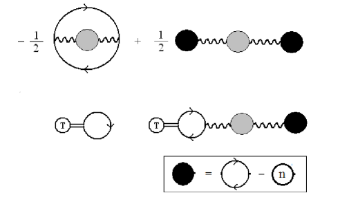
Figure 2: The graphic representation of the sum of the Feynman diagrams associated to contributions linked with the vertices of the total Hamiltonian. The insertion at the bottom symbolize the total particle density (black disk) as defined by the sum of the electron density (the closed propagator line) minus the density of charged particles in the nuclei (the circle with an interior letter ”$n$”). For homogeneous systems in which the jellium is homogeneous and the electron full translation symmetry is not broken, this total density vanishes.

The generic types of connected contributions satisfying the screening approximation are illustrated in figure 2.  The first series corresponds to the addition of an infinite number of self-energy insertions of the fermion polarization loops in the Coulomb interaction line of the standard $HF$ exchange term. The grey circles with attached wavy lines represents screened potential resulting from the described insertions. The second series corresponds to the sum of an arbitrary number of such insertions of the polarization loop in the Coulomb interaction line of the standard direct term in the HF scheme.  As defined before, this total density is the electron particle density minus the density of the nuclear charged particles.  This direct term includes the geometric series of polarization insertions in the Coulomb interaction between: the electron charges among themselves, the nuclear ”jellium” charges among them and the interaction between these two kind of charges. The last four  terms combined correspond to  screening contributions to the mean value of the kinetic energy, which are mainly determined by the total charge density. Each contribution having a given number $\ l$ of fermion polarization loops in its diagram has a sign $(-1)^{l}$.  The geometric series over all the insertions in the graphs of figure 2 reproduces the usual definition of the screened Coulomb potential kadanoff ; thouless .

The polarization loops in the graphic have the expressions

$$P(x,x^{\prime}) =\frac{-i}{\hbar}G(x,x^{\prime})G(x^{\prime},x)$$

$$=\int\varphi{}_{l}(\mathbf{x})\varphi_{l}^{\ast}(\mathbf{x}^{\prime})\varphi_{k}^{\ast}(\mathbf{x}^{\prime})\varphi_{k}^{\ast}(\mathbf{x})\exp(-i\text{ }w(t-t^{\prime}))\times$$

$$\frac{2}{\hbar}\frac{f_{k}-f_{l}}{(w+\frac{1}{\hbar}(\epsilon_{k}-\epsilon_{l})+i\text{ }\alpha(f_{k}-f_{l})\text{ }},$$ (29)

$$f_{k} =\theta(\epsilon_{f}-\epsilon_{k}),$$ (30)

and the screened Coulomb potential arising form the summation of the geometric series of polarization insertions is given as

$$v^{s}(x,x^{\prime}) =v_{c}(x,x^{\prime})-\int dx_{1}dx_{2}v_{c}(x,x_{1})P(x_{1},x_{2})v_{c}(x_{2},x^{\prime})+$$

$$\int dx_{1}dx_{2}dx_{3}dx_{4}v_{c}(x,x_{1})P(x_{1},x_{2})v_{c}(x_{2},x_{3})P(x_{3},x_{4})v_{c}(x_{4},x^{\prime})+...$$

$$(-1)^{n}\int dx_{1}dx_{2}dx_{3}dx_{4}...dx_{2n-1}dx_{2n}v_{c}(x,x_{1})P(x_{1},x_{2})v_{c}(x_{2},x_{3})P(x_{3},x_{4})v_{c}(x_{4},x^{\prime})...$$

$$v_{c}(x,x_{2n-1})P(x_{2n-1},x_{2n})v_{c}(x_{2n},x^{\prime})$$

$$=(v_{c}\frac{1}{1+Pv_{c}})(x,x^{\prime})$$

$$=(\frac{1}{1+v_{c}P}v_{c})(x,x^{\prime})$$

$$=\int dx_{1}\text{ }\varepsilon(x,x_{1})v_{c}(x_{1},x^{\prime}),$$ (31)

in which the usual definition $\varepsilon(x,x$´$)$ of the dielectric function in the screened approximation appears kadanoff .

The screening effect on the kinetic energy can be expressed in terms of a correction to the electron propagator including all the self-energy insertions of the total potential generated by the total charge density $\rho_{t}$, as follows. This screening modified Green function

$$G^{s}(x,x^{\prime}) =G(x,x^{\prime})+\int dx_{1}G(x,x_{1})(\frac{-i}{\hbar})V_{t}(x_{1})G(x_{1},x^{\prime})+$$

$$\int dx_{1}\int dx_{2}G(x,x_{1})(\frac{-i}{\hbar})V_{t}(x_{1})G(x_{1},x_{2})(\frac{-i}{\hbar})V_{t}(x_{2})G(x_{2},x^{\prime})+...$$

$$\int dx_{1}\int dx_{2}G(x,x_{1})(\frac{-i}{\hbar})V_{t}(x_{1})G(x_{1},x_{2})...(\frac{-i}{\hbar})V_{t}(x_{n})G(x_{n},x^{\prime})...$$

$$=(G\frac{1}{1-(\frac{-i}{\hbar})V_{t}G})(x,x^{\prime})$$

$$=(\frac{1}{1-GV_{t}(\frac{-i}{\hbar})}G)(x,x^{\prime}),$$ (32)

$$V_{t}(x) =\int dx\acute{}v^{s}(x,x\acute{})\rho_{t}(x\acute{}),$$ (33)

$$\rho_{t}(x) =G(x,x^{+})+\rho_{n}(x),$$ (34)

$$x^{+} =(\overrightarrow{x},t+\delta),\text{ \ \ }\delta=0^{+}.$$

where the addition of a small infinitesimal positive number $\delta$ to the time component of a four-vector $x$ has been indicated as $x^{+}=(\overrightarrow{x},t+\delta),$   $\delta=0^{+}.$ Finally the analytic expression for the functional $E$ can be written in the form

$$E =-\frac{1}{2}\int dxdx^{\prime}G(x,x^{\prime})G(x^{\prime},x)v^{s}(x,x^{\prime})+$$

$$\frac{1}{2}\int dxdx^{\prime}\rho_{t}(x)v^{s}(x,x^{\prime})\rho_{t}(x^{\prime}))+$$

$$\int dxdx^{\prime}{\large(}\frac{-\hbar^{2}}{2m}\mathbf{\nabla}_{x}^{2}G(x,x^{\prime}){\Large|}_{x^{\prime}->x^{+}})G^{s}(x^{\prime},x),$$ (35)

in which all the participating elements are functionals of the  basis functions $\varphi_{k}$ through the propagator $G(x,x^{\prime})$ as follows

$$v^{s}(x,x^{\prime}) =(v_{c}\frac{1}{1+Pv_{c}})(x,x^{\prime})$$ (36)

$$G^{s}(x,x\text{\'{}}) =(G\frac{1}{1-(\frac{-i}{\hbar})V_{t}G})(x,x^{\prime})$$ (37)

$$P(x,x\acute{}) =\frac{-i}{\hbar}G(x,x^{\prime})G(x^{\prime},x)$$ (38)

$$V_{t}(x) =\frac{-i}{\hbar}\int dx\,v^{s}(x,x\acute{})\rho_{t}(x\acute{})$$ (39)

$$\rho_{t}(x) =G(x,x^{+})+\rho_{n}(x)$$ (40)

$$G(x,x^{\prime}) =\int\frac{dw}{2\pi}\sum_{k}\frac{i\text{ }\varphi_{k}(\mathbf{x})\varphi_{k}^{\ast}(\mathbf{x}^{\prime})\exp(-i\text{ }w(t-t^{\prime}-\delta))}{(w-\frac{1}{\hbar}\epsilon_{k}+i\text{ }\alpha\text{ }sgn(\epsilon_{k}-\epsilon_{f}))}$$ (41)

$$sgn(a) =\theta[a]-\theta[-a].$$ (42)

Let us write the variational equations for the single particle wavefunctions $\ \varphi_{k}(x)$ in next subsection.

II.4 The equations for the single particle states

As usual, the set of equations for determining the basis functions  $\varphi_{k}(x)$ will be written as the vanishing derivatives of a Lagrange functional  with respect to all the functions, by also imposing on them the orthonormality constraints.  Since $E$ is a functional of the $\varphi_{k}(x)$ only through its dependence on the fermion Green functions, the chain rule for the functional derivatives is helpful. Then, the following expression for the derivative of $G$ with respect to any of the conjugate one particle wavefunctions can be employed

$$\frac{\delta}{\delta\varphi_{k}^{\ast}(\mathbf{x}^{\prime\prime})}G(x,x^{\prime}) =\varphi_{k}(\mathbf{x})\text{ }\delta^{(3)}(\mathbf{x}^{\prime\prime}-\mathbf{x}^{\prime})f_{k}(t-t^{\prime})$$

$$f_{k}(t-t^{\prime})= (\theta(t-t^{\prime}-\delta)\theta(\epsilon_{k}-\epsilon_{f})-\theta(t^{\prime}-t+\delta)\theta(\epsilon_{f}-\epsilon_{k})\times$$ (43)

$$.\exp(-i\frac{\epsilon_{k}}{\hbar}(t-t^{\prime}-\delta).$$ (44)

That is, the functional derivative of $G$  with respect to $\varphi_{k}(x),$ is proportional to the wavefunction at the same quantum number, as multiplied by an energy dependent factor of unit absolute value and by a Dirac Delta function. The Delta function when integrated over an internal variable $\mathbf{x}^{\prime}$ will define $\mathbf{x}^{\prime\prime}$ as the external point of the diagram. The point $\mathbf{x}$ will be the one at the other extreme of  fermion line where the arrow arrives to the point to in which the wavefunction $\varphi_{k}$ is evaluated.  Employing the Lagrange multipliers method to  find the extremal of $E$ by also imposing the orthonormality  constraints on the functions $\varphi_{k},$ the  effective  functional  $E_{Lag}$ to be used for writing the equations for the extremals, will be

$$E_{Lag}=E-\sum_{l\neq k}\lambda_{kl}\text{ }(\int d\mathbf{x}\text{ }\varphi_{k}^{\ast}(\mathbf{x})\varphi_{l}(\mathbf{x})-\delta_{kl}).$$ (45)

where $\lambda_{kl}$ are the Lagrange multipliers of the imposed orthonormality constraints.   Note that, the not yet specified energies $\epsilon_{k}$ defining the free Hamiltonian $H_{0},$ are not yet  related with the Lagrange multipliers $\lambda_{kl}$.    Then, the above rule for the derivative of the propagators, allows to write the extremum condition for $E_{Lag}$ in the form

$$\frac{\delta}{\delta\varphi_{k}^{\ast}(\mathbf{x})}E_{Lag} =0$$

$$=\int d\mathbf{x}^{\prime}H_{Fock}(\mathbf{x},\mathbf{x}^{\prime})\varphi_{k}(\mathbf{x}^{\prime})-\sum_{l\neq k}\lambda_{kl}\text{ }\varphi_{l}(\mathbf{x}),$$ (46)

$$\frac{\delta}{\delta\lambda_{kl}^{\ast}(\mathbf{x})}E_{Lag} =\int d\mathbf{x}\text{ }\varphi_{k}^{\ast}(\mathbf{x})\varphi_{l}(\mathbf{x})-\delta_{kl}=0,$$ (47)

in which  the modified Fock kernel including screening effects is written in the form

$$H_{Fock}(\mathbf{x},\mathbf{x}^{\prime}) =T(\mathbf{x},\mathbf{x}^{\prime})+V_{ex}^{k}(\mathbf{x},\mathbf{x}^{\prime})+V_{dir}^{k}(\mathbf{x},\mathbf{x}^{\prime})+$$ (48)

$$V_{s}^{k}(\mathbf{x},\mathbf{x}^{\prime})+^{(1)}V_{T-v}^{k}(\mathbf{x},\mathbf{x}^{\prime})+^{(2)}V_{T-v}^{k}(\mathbf{x},\mathbf{x}^{\prime}).$$ (49)

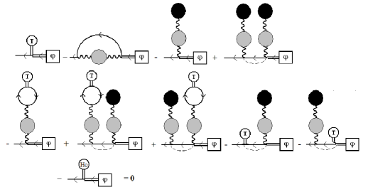
Figure 3: The picture illustrates the set of generalized HF equations for the single particle states. They follows after taking the derivative of the energy functional over the conjugate of the single particle wavefunctions at the space point represented by the external left end of each graphic. The squares with an interior $\varphi$ represent the single particle orbitals being searched. The figures connected with them represent the various kernels defining the generalized Fock operator in expression  48. The dashed lines represent the time and quantum number dependent functions $f_{k}(t-t^{\prime})$. The time integrals over these functions, in combination with the time invariance symmetry implements the time independence of the Fock operator.

The various kernels appearing in the above expression have the explicit forms

$$T(\mathbf{x},\mathbf{x}^{\prime}) =-\frac{\hbar^{2}}{2m}\theta(\epsilon_{f}-\epsilon_{k})\mathbf{\nabla}_{x}^{2}\delta(\mathbf{x-x}^{\prime}),$$ (50)

$$V_{ex}^{k}(\mathbf{x},\mathbf{x}^{\prime}) =\frac{1}{T}\int dt\text{ }dt^{\prime}f_{k}(t-t^{\prime})G(\mathbf{x},t,\mathbf{x}^{\prime},t^{\prime})v_{s}(\mathbf{x},t,\mathbf{x}_{4},t_{4})\varepsilon(\mathbf{x}_{4},t_{4},\mathbf{x}^{\prime},t^{\prime}),$$ (51)

$$V_{dir}^{k}(\mathbf{x},\mathbf{x}^{\prime}) =-\theta(\epsilon_{f}-\epsilon_{k})v_{t}(x)\delta(\mathbf{x-x}^{\prime})$$ (52)

$$V_{s}^{k}(\mathbf{x},\mathbf{x}^{\prime}) =\frac{i}{h}\int dt\text{ }dt^{\prime}f_{k}(t-t^{\prime})v_{t}(x)G(x,x^{\prime})v_{t}(x^{\prime})\rho_{t}(x^{\prime}),$$ (53)

$$v_{t}(x^{\prime}) =\int v_{s}(x,x^{\prime\prime})\rho_{t}(x^{\prime\prime})dx^{\prime\prime}$$ (54)

$$V_{T}^{k}(\mathbf{x},\mathbf{x}^{\prime}) =-\delta(\mathbf{x-x}^{\prime})\int dx^{\prime}v_{s}(x,x_{2})G(x_{2},x_{3})(-\frac{\hbar^{2}}{2m})\mathbf{\nabla}_{\overrightarrow{x}_{3}}^{2}G(x_{3},x_{2}))$$ (55)

$${}^{(1)}V_{T-v}^{k}(\mathbf{x},\mathbf{x}^{\prime}) =-\int dt\int dt^{\prime}dx_{2}dx_{3}\text{ }f_{k}(t-t^{\prime})v_{s}(x,x_{2})G(x_{2},x_{3})(-\frac{\hbar^{2}}{2m})\mathbf{\nabla}_{\overrightarrow{x}_{3}}^{2}G(x_{3},x_{2})\times$$

$$G(x,x^{\prime})v_{t}(x^{\prime})+$$ (56)

$$\text{ \ \ \ \ \ \ }\int dt\int dt^{\prime}dx_{2}dx_{3}\text{ }v_{t}(x)f_{k}(t-t^{\prime})G(x,x^{\prime})v_{s}(x^{\prime},x_{2})G(x_{2},x_{3})(-\frac{\hbar^{2}}{2m})\mathbf{\nabla}_{\overrightarrow{x}_{3}}^{2}G(x_{3},x_{2})$$ (57)

$${}^{(2)}V_{T-v}^{k}(\mathbf{x},\mathbf{x}^{\prime}) =-\int dt\int dt^{\prime}\text{ }f_{k}(t-t^{\prime})(-\frac{\hbar^{2}}{2m})\mathbf{\nabla}_{\overrightarrow{x}}^{2}G(x,x^{\prime})v_{t}(x^{\prime})$$

$$-\int dt\int dt^{\prime}\text{ }v_{t}(x)f_{k}(t-t^{\prime})G(x,x^{\prime})(-\frac{\hbar^{2}}{2m})\mathbf{\nabla}_{\overrightarrow{x^{\prime}}}^{2}$$ (58)

The equations for the single particle wavefunctions are graphically illustrated in figure 3. It should be noted that the electron, nuclear and total particle densities are constant, thus the total potential $V_{t}$ is also time independent.

At this point we will specify the spectrum of the free Hamiltonian $H_{0}$.  The most natural way we estimate for choosing it, seems to require that these energies coincide with the solutions for the diagonal components of the matrix of eigenvalues $\lambda_{kl}$, which are defining by the extremum problem (as functions of the spectrum {$\epsilon_{k}\}$). This selection is suggested, by the fact that in this case, the free quantum mechanical problem defined by $H_{0}$, will have an energy, at the extremum solution for the single particle wavefunctions, which exactly coincides with the value of the optimized functional $E$.

II.5 The homogeneous electron systems

Let us assume now that the electronic system under consideration is homogeneous. Then, the quantum numbers $k$ can be taken in form $\ k=\mathbf{p}=(\overrightarrow{p},\sigma_{z})$, in terms of the spacial momenta and the projections of the spin in a given direction. The normalized wavefunctions in a large box of volume $V$ are the plane waves. The amplitudes $\varphi_{\mathbf{p}}$will have a spin dependence implicitly assumed

$$\varphi_{\mathbf{p}}(\mathbf{x})=\frac{1}{V}\varphi_{\mathbf{p}}\exp(i\text{ }\overrightarrow{p}.\overrightarrow{x}).$$ (59)

Since the Lagrangian multipliers with different indices vanish as follows form the Lagrange extremum conditions, after defining $\lambda_{\mathbf{p}}=\lambda_{\mathbf{pp}}=\epsilon(\mathbf{p})\equiv k$, the HF equations  take the simple form

$$H_{Fock}(\mathbf{p})\varphi_{\mathbf{p}} =\lambda_{\mathbf{p}}\text{ }\varphi_{\mathbf{p}},$$ (60)

$$H_{Fock}(\mathbf{p}) =T(\mathbf{p})+V_{ex}^{\mathbf{p}}(\mathbf{p}),$$

where the Hamiltonian  is the sum of the following constants defined by the Fourier transforms of the potential

$$T(\mathbf{p}) =\frac{\hbar^{2}}{2m}\theta(\epsilon_{f}-\epsilon_{\mathbf{p}})\overrightarrow{p}^{2},$$ (61)

$$V_{ex}^{\mathbf{p}}(\mathbf{p}) =\frac{1}{T}\int d\overrightarrow{x}\int d\tau\text{ }\exp(-i\text{ }\overrightarrow{p}.\overrightarrow{x})\int dt\text{ }dt^{\prime}f_{k}(t-t^{\prime})G(\mathbf{x},t,\mathbf{x}^{\prime},t^{\prime})v_{s}(\mathbf{x},t,\mathbf{x}_{4},t_{4})\varepsilon(\mathbf{x}_{4},t_{4},\mathbf{x}^{\prime},t^{\prime}),$$ (62)

$$\varepsilon(x,x^{\prime}) =(\frac{1}{1+v_{c}P})(x,x^{\prime}).$$ (63)

Note that various potential terms in the general inhomogeneous case are not appearing because in the homogeneous electron systems, the ”jellium” nuclear charge should rigorously cancel the electron charge for the system to be homogeneous. The vanishing of one of these terms, in which the total density is not appearing, also follows after being directly evaluated. The electron Green function in momentum space is

$$G(\mathbf{p},w) =\frac{\exp(i\text{ }w\text{ }\delta)}{i(w-\frac{1}{\hbar}\epsilon_{\mathbf{p}}+i\text{ }\alpha\text{ }sgn(\epsilon_{\mathbf{p}}-\epsilon_{f}))},$$ (64)

$$\delta \rightarrow 0^{+},$$

and the screening potential as a function of the polarization is given by

$$v^{s}(p) =v_{c}(p)-v_{c}(p)P(p)v_{c}(p)+$$

$$v_{c}(p)P(p)v_{c}(p)P(p)v_{c}(p)+...$$

$$(-1)^{n}v_{c}(p)P(p)v_{c}(p)P(p)v_{c}(p)...$$

$$v_{c}(p)P(p)v_{c}(p)$$

$$=\frac{v_{c}(p)}{1+P(p)v_{c}(p)}$$

$$=\varepsilon(p)v_{c}(p),$$ (65)

$$v_{c}(p) =\frac{4\pi e^{2}}{\overrightarrow{p}^{2}}.$$ (66)

Finally, the Fourier transform of the polarization function can be evaluated as follows

$$P(\overrightarrow{q},w) =\frac{1}{\hbar}\int d(\overrightarrow{x}-\overrightarrow{x}^{\prime})d(t-t^{\prime})\exp(-i\text{ }\overrightarrow{q}.(\overrightarrow{x}-\overrightarrow{x}^{\prime})+i\text{ }w.(t-t^{\prime}))G(x-x^{\prime})G(x^{\prime}-x)$$

$$=\sum_{\mathbf{k}}\frac{1}{V}\frac{2}{\hbar}\frac{f_{\overrightarrow{\mathbf{k}}}-f_{\overrightarrow{\mathbf{k}}+\overrightarrow{\mathbf{q}}}}{(w+\frac{1}{\hbar}(\epsilon_{\mathbf{k}}-\epsilon_{\overrightarrow{\mathbf{k}}+\overrightarrow{\mathbf{q}}})+i\text{ }\alpha\text{ (}f_{\overrightarrow{\mathbf{k}}}-f_{\overrightarrow{\mathbf{k}}+\overrightarrow{\mathbf{q}}}\text{)}}$$ (67)

$$=\int\frac{d\overrightarrow{k}}{(2\pi)^{3}}\frac{2}{\hbar}\frac{f_{\overrightarrow{\mathbf{k}}}-f_{\overrightarrow{\mathbf{k}}+\overrightarrow{\mathbf{q}}}}{(w+\frac{1}{\hbar}(\epsilon_{\mathbf{k}}-\epsilon_{\overrightarrow{\mathbf{k}}+\overrightarrow{\mathbf{q}}})+i\text{ }\alpha\text{ (}f_{\overrightarrow{\mathbf{k}}}-f_{\overrightarrow{\mathbf{k}}+\overrightarrow{\mathbf{q}}}\text{)}},$$ (68)

$$\int\frac{d\overrightarrow{k}}{(2\pi)^{3}} \approx\sum_{\mathbf{k}}\frac{1}{V}.$$ (69)

II.6 Iterative solution for the electron self-energies in the static limit

In this subsection we now iteratively solve the set of self-consistent equations for the electron orbitals.   In order to simplify the evaluation, we will  assume the validity of the static approximation. That is, the polarization at all frequencies $P(\overrightarrow{q},w)$ will be substituted by its value at zero frequency $P(\overrightarrow{q},0)$  In other words, the effective potential will act  in the same instantaneous way as the  Coulomb potential does. In what follows, in order to simplify the notation we will not use the combined space-spin momenta notation $\mathbf{p}$=$(\overrightarrow{p},s)$ which is however helpful in less symmetric problems.

The self-consistent  connection between the quantities can be described as follows. Firstly, the screened Coulomb potential can be evaluated from the frequency independent formula

$$v_{s}(p)=v_{s}(\overrightarrow{p})=\frac{v_{c}(\overrightarrow{p})}{1+P(\overrightarrow{p}\mathbf{,}0)v_{c}(\overrightarrow{p})},$$ (70)

in terms of the known Coulomb potential $v_{c}$ and the frequency independent polarization expression

$$P(\overrightarrow{q},0)=\frac{2}{\hbar}\int\frac{d\overrightarrow{k}}{(2\pi)^{3}}\frac{\theta(k_{f}-k)-\theta(k_{f}-|\overrightarrow{k}+\overrightarrow{q}|)}{\frac{1}{\hbar}(\epsilon_{k}-\epsilon_{\overrightarrow{k}+\overrightarrow{q}})+i\text{ }\alpha\text{ }(\theta(k_{f}-k)-\theta(k_{f}-|\overrightarrow{k}+\overrightarrow{q}|)},$$ (71)

which is fully defined in terms of the energy spectrum $\{\epsilon_{k}\}.$  Then, this set of energies can be determined again in terms of the screened potential $v_{s}$ by means of solving the Fock Hamiltonian equations

$$H_{Fock}(\overrightarrow{p})\varphi_{\overrightarrow{p}} =\epsilon_{\overrightarrow{p}}\text{ }\varphi_{\overrightarrow{p}},$$ (72)

$$H_{Fock}(\overrightarrow{p}) =\frac{\hbar^{2}\overrightarrow{p}^{2}}{2m}+V_{ex}^{\overrightarrow{p}}(\overrightarrow{p}),$$ (73)

$$V_{ex}^{\overrightarrow{p}}(\overrightarrow{p}) =-\int\frac{d\overrightarrow{k}}{(2\pi)^{3}}\theta(k_{f}-k)\theta(k_{f}-|\overrightarrow{k}+\overrightarrow{q}|)\varepsilon(\overrightarrow{p})v_{s}(\overrightarrow{p}).$$ (74)

In a more detailed form, firstly we choose the Coulomb  potential $v_{c}$ as the first approximation for  $v_{s}$ in the Fock Hamiltonian equations, to determine the first approximation for the energy spectrum. Next, the single particle energies defined in this approximation, are used to evaluate the polarization $P(\overrightarrow{p},0),$ and with this quantity, a new approximation for the screened potential $v_{s}$ is calculated.  Afterwards, knowing $v_{s}$,  the same cycle is repeated again iteratively up to arriving to stable values of the three quantities $P(\overrightarrow{p},0),$ $v_{s}(\overrightarrow{p})$ and $\epsilon_{\overrightarrow{p}}$.

For the homogeneous electron gas the Fermi momentum $k_{f}$ , defined by

$$N=\frac{2V}{(2\pi)^{3}}\frac{4\pi}{3}k_{f}^{3},$$

will  fully determine the properties of the solution.  It can be defined as usual, the mean radius per particle $r_{0},$ in terms of the volume of the gas $V$ and the number of particles $N_{p}$ by $\ V=N_{p}\frac{4\pi}{3}r_{0}^{3}$ . Then, the Fermi wavevector $k_{f}$ expresses in terms of $r_{0}$  in the form

$$k_{f}=\frac{1}{(\frac{4}{9\pi})^{\frac{1}{3}}r_{0}}.$$

Given the Bohr radius expression $a_{B}$=$\frac{\hbar^{2}}{me^{2}},$ the value of $k_{f}$  that was be chosen for the calculation was

$$k_{f}\text{ }a_{B}=\frac{1}{(\frac{4}{9\pi})^{\frac{1}{3}}}\frac{a_{B}}{r_{0}}=1.$$

That is, the electron gas density is assumed to be close to one electron within the volume of a sphere having as its radius $a_{B}$. The  expression of the  self-energies in the first step of the iterative process, is obtained assuming that the $v_{s}$ coincides with the Coulomb potential, that is $v_{s}(\overrightarrow{k})=v_{c}(\overrightarrow{k}).$ Then, the exchange ${}^{(1)}V_{ex}^{\overrightarrow{p}}(\overrightarrow{p})$ and the total $\epsilon_{\overrightarrow{p}}^{(1)}$ energies coincide with usual $HF$ results

$${}^{(1)}V_{ex}^{\overrightarrow{p}}(\overrightarrow{p}) =-\int\frac{d\overrightarrow{k}}{(2\pi)^{3}}\theta(k_{f}-k)\theta(k_{f}-|\overrightarrow{k}+\overrightarrow{q}|)v_{c}(\overrightarrow{p})$$ (75)

$$=-\frac{e^{2}}{2\pi}(\frac{k_{f}^{2}-p^{2}}{p}\log(|\frac{k_{f}+p}{k_{f}-p}|)+2k_{f}),$$ (76)

$$\epsilon_{\overrightarrow{p}}^{(1)} =\frac{\hbar^{2}\overrightarrow{p}^{2}}{2m}-\frac{e^{2}}{2\pi}(\frac{k_{f}^{2}-p^{2}}{p}\log(|\frac{k_{f}+p}{k_{f}-p}|)+2k_{f}).$$ (77)

Afterwards, the first iterative value of the polarization $P^{(1)}(\overrightarrow{p},0)$, was evaluated with the use of (71) by substituting in this expression the spectrum $\epsilon_{\overrightarrow{p}}^{(1)}$  in  (77).   The values of $P^{(1)}(\overrightarrow{p},0)$ obtained were then employed to evaluate the first iterative values of the  screened potential $v_{s}^{(1)}(\overrightarrow{p})$ through formula (70).

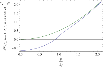
Figure 4: The figure shows the single particle energy spectra for the four iterations done in the solving the generalized HF equations. The system considered corresponds to an inter-electron mean distance close to the Bohr radius. The energy dependence in the first step of the iterative values of the energy coincides with the HF result and corresponds to the lower curve. The convergence of the iterative process is rapid, as indicated by the almost coincidence in the spectra for the next tree iterations, which are given by the three upper almost identical plots.

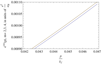
Figure 5: The figure illustrates the small difference between the resulting energy spectra of the second and third iterations done in evaluating the energies. The spectrum following in the fourth iteration is also shown, but is not evident, because almost coincides with the result of the third iteration.

Henceforth, the function $v_{s}^{(1)}(\overrightarrow{p}),$  allowed to start the cycle again, to find the similar quantities in the second step $\epsilon_{\overrightarrow{p}}^{(2)},P^{(2)}(\overrightarrow{p},0)$   and $v_{s}^{(2)}(\overrightarrow{p})$ through the same procedure followed before.

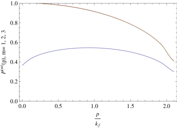
Figure 6: The figure shows the results for the static polarization $P$ in the three iterations in which it was evaluated. Again, the difference between the second an the third iteration (corresponding to the two superposed upper curves) can not be noticed in the scale of the graphic.

The described cycles were repeated three times, after which the evaluated quantities closely approached to self-consistent values of the functions $V_{ex}^{\overrightarrow{p}}(\overrightarrow{p}),\epsilon_{\overrightarrow{p}},P(\overrightarrow{p},0)$   and $v_{s}(\overrightarrow{p}).$  The third iteration for the screened potential allowed to evaluate one further iteration for the energy, which explains the number of four plotted curves in figure 4. The  results for these quantities in the various steps  are illustrated  in figures 4-7.

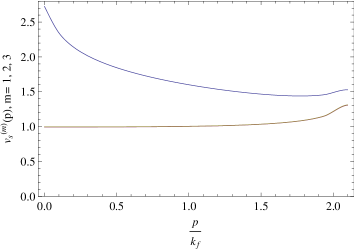
Figure 7: The figure shows the three iterative results evaluated for the screened potential. As for the other plots the differences between the second and third iterations (associated to the coinciding lower two plots) can not be noticed. They indicate that the amount of screening predicted for the considered electron density is high. This can be also noticed form the spectra shown in figure 4, which shows a large reduction of the exchange energy of the usual HF solution. Since the screening properties had been assumed in the static approximation, is not clear whether this reduction of the exchange energy will also appears when the exact dynamic screening effects will be considered.

The  plots in each of these pictures show the  values of the quantities in the  few steps which were required to  attain convergence.   It followed that the energies, and screening potentials rapidly attain their selfconsistent values after two steps of the iteration process.  In all of the pictures 4, 6 and 7, the differences between the second, and third iterations can not be noticed.

Figure 4 illustrates the outcome for single particle energy spectra for the four iterations done in the solving the generalized HF equations. The system considered corresponds to an inter-electron mean distance being close to the Bohr radius. The energy dependence of the first iteration, coincided with the HF result.  Figure 5 gives an augmented picture of the energies of the last two iterations in the low momentum region. It is shown to evidence the rapid convergence of the procedure.  The energy associated to the second, third and fourth are shown, but the third and the fourth, do not differentiate in the scale of the figure.

Figures 6 and 7 show the results for the polarization $P(\overrightarrow{p},0)$ and the screened potential $v_{s}(\overrightarrow{p})$. The plots indicate that the amount of screening at the considered electron density is high. This can be also noticed from the spectra shown in figure 4, which evidences a large reduction of the exchange energy of the usual HF solution. However, since the screening properties in the present exploratory study, had been assumed in the static approximation, is not clear whether or not this effect will also appears when the exact dynamic screening effects will be considered.  This question is expected to be considered elsewhere.

The calculations done in the work referred to homogeneous systems and a very particular value of the density, in order to simply illustrate the implementation of the procedure. With this same purpose the strong static approximation for the polarization properties was also assumed. However, a further investigation of the homogeneous systems is yet a subject of appreciable physical interest and it is expected to be considered elsewhere. In particular, the inclusion of the dynamic screening effects could  modify the results for the energy, which are higher than the HF ones. Finally, it can be noted that the derivative of the energy dispersion at the Fermi  momentum $k_{f}$ is finite in the solution, thus eliminating this known difficulty of the HF self-energy spectrum  kittel .

III Conclusions

A generalization of the self-consistent Hartree Fock procedure including screening effects was introduced. Expressions for the HF like functional and its system of self-consistent equations are presented.  For inhomogeneous electron systems, the equations include additional terms to the standard direct and exchange potentials.  The presence of the nuclear charge is included in the scheme, seeking to allow its further application in the developing of band calculation procedures. To start exploring the implementation of the analysis, it is applied to the homogeneous electron gas.  The system HF equations is then iteratively solved in the further simplified case of assuming that the dielectric properties are taken in the unretarded approximation. The electron density is fixed to be approximately correspond to one Bohr radius mean inter-electron distance. The system of equations is solved iteratively by approximating, the screened potential by the Coulomb one in evaluating the first iteration for the spectrum for the electron energies. Afterwards, the screened potential and the new spectrum determined by it, were recursively calculated. The results indicate that in the non retarded approximation, both the direct and the exchange potential are strongly screened. Therefore the energy spectrum behaves very closely to the free electron one. Thus, the the non retarded approximation does not produce an improvement in lowering the energy of the standard HF procedure. The possibility for such an improvement was a central motivation for the present work. However, the non retardation assumption is a dynamical simplification which is not necessarily compatible with the (not shown here, but expected to be valid) variational character of the scheme. Therefore, the hope exist, that after performing a similar iterative solution, but without assuming the static approximation for the fermion loops, can produce an energy competing with the the standard HF one. This iterative solution, is not very much difficult than the one done in this work. Thus, if it becomes able to furnish an energy competing with the HF one, the method could become a helpful one. The existence of sum rules for the frequency dependent dielectric quantities rises the expectation about they could incorporate lowering energy contribution, possibly becoming able to contest with the exchange energy in the usual HF scheme of the homogeneous electron gas. This question will be investigated in the next extension of the work.

One point to be underlined is that in the homogeneous electron gas, it is known that the $HF$ scheme predicts a non physical vanishing density of states at the Fermi level kittel ; madelung ; raimes ; callaway ; zerodensity , it is clear that this property is eliminated in there result of the iterative process in the proposed scheme.

It should be also remarked that the present work, had been motivated, precisely by the idea of deriving in its further extension, the crystal symmetry breaking and spin-space entanglement effects obtained in Ref. symmetry for $La_{2}CuO_{4}$.  In these works, a simple model of the CuO planes was constructed.  It was defined by a set Coulomb interacting electrons, for which the free Hamiltonian was taken as a Tight Binding one. The electrons were assumed to half fill a single Tight Binding band.  The lattice of the model was chosen as the 2D crystal formed by the Cu atoms in the CuO planes. The Coulomb interaction in the system was then considered in the HF approximation. In the study, a phenomenological value of the dielectric constant of nearly $\varepsilon=10$ was assumed to screen the Coulomb interaction. This consideration was done in order to match the width of the $HF$ spectrum of the Coulomb interacting electrons, with the width of the single half filled band crossing the Fermi level, arising in the Matheiss full band structure calculation in Ref. matheiss . After that, by simply eliminating some usually imposed symmetry constraints on the HF procedure, a fully unrestricted HF solution of the HF problem predicted an insulator gap and the antiferromagnetic structure for the $La_{2}CuO_{4}$, which are considered as pure strong correlation effects in the material.

The above circumstances, also motivated the idea of constructing a full $HF$ band calculation scheme, eventually being able to predict the assumed dielectric screening in Ref. symmetry ,  by also incorporating the mentioned crystal symmetry breaking and spin-spacial entanglement effects, in describing the Mott strong correlation properties of the $La_{2}CuO_{4}$ material. The possibility to derive the above mentioned (just fitted in symmetry ) dielectric constant, is suggested by the following circumstance.  The usual $HF$ band structure evaluations of the $La_{2}CuO_{4}$ are known to predict an enormous band gap of nearly $17$ eV su . However, after dividing this energy gap by the value of $10$ for the dielectric constant employed in the described model of CuO planes, gives a result of $1.7$ eV, which is close to the measured gap of the $La_{2}CuO_{4}$ of $2$ eV. Then, the expectation arises that a band calculation scheme based in the proposed modified HF scheme, could work in predicting the main strong correlation properties of the $La_{2}CuO_{4}$, and eventually of  its close related transition metal oxides. The investigation of these possibilities is expected to be considered elsewhere.

- (1) N. F. Mott. Proc. Phys. Soc., London, A62:416, 1949.
- (2) J. C. Slater. Phys. Rev., 81(3).
- (3) J. C. Slater. Quantum Theory of Atomic Structure, volume 2. Dover Publications Inc., Mineola, New York., 1960.
- (4) J. G. Bednorz y K. A. Müller. Rev. Mod. Phys., 60:585, 1987.
- (5) E. Dagotto. Rev. Mod. Phys., 66:763, 1994.
- (6) C. Almasan y M. B. Maple. Chemistry of High Temperature Superconductors. World Scientific, Singapore, 1991.
- (7) Y. Yanase. Physics Reports, 387:1, 2003.
- (8) D. J. Van Harlingen. Rev. Mod. Phys., 67:515, 1995.
- (9) A. Damascelli. Rev. Mod. Phys., 75, 2003.
- (10) W. E. Pickett. Rev. Mod. Phys., 61:2, 1999.
- (11) G. Burns. High-Temperature Superconductivity. Academic, New York..
- (12) M. Imada. Rev. Mod. Phys., 70(4), 1998.
- (13) G. Shirane D. E. Moncton S. K. Sinha S. Vaknin J. P. Remeika A. S. Cooper y D. Harshman T. J. Freltoft, J. E. Fischer. Phys. Rev., B36:826, 1987.
- (14) J. H. de Boer y E. J. W. Verway. Proc. Phys. Soc., London, A49:94, 1937.
- (15) R. Peierls. Proc. Phys. Soc., London, A49:72, 1937.
- (16) P. W. Anderson. Phys. Rev., 115:2, 1959.
- (17) F. Hubbard. Proc. R. Soc., London, A276:238, 1963.
- (18) P. W. Anderson. Science, 235:1196, 1987.
- (19) E. Fradkin. Field Theories of Condensed Matter, volume 82. Addison Wesley Publishing Company, 1991.
- (20) M. Gutzwiller. Phys. Rev., A134:923, 1964.
- (21) M. Gutzwiller. Phys. Rev., A137:1726, 1965.
- (22) W. F. Brinkman y T. M. Rice. Phys. Rev., B2:4302, 1970.
- (23) W. Kohn. Phys. Rev., A133:171, 1964.
- (24) W. Kohn y L. J. Sham. Phys. Rev., A140:1133, 1965.
- (25) A. R. Williams y N. Hamada K. Terakura, T. Oguchi. Phys. Rev. Lett., 52:1830, 1984.
- (26) D. J. Singh y W. E. Pickett. Phys. Rev., B44:7715, 1991.
- (27) A. Szabo y N. Ostlund. Modern Quantum Chemistry: Introduction to Advanced Electronic Structure Theory. Dover Publications Inc., Mineola, New York., 1989.
- (28) A. L. Fetter y J. D. Walecka. Quantum Theory of Many Particle Physics, volume 1. McGraw-Hill, Inc., 1971.
- (29) L. F. Matheiss. Phys. Rev. Lett., 58:1028, 1987.
- (30) N. F. Mott. Metal-Insulator Transition. Taylor and Francis, London/Philadelphia, 1990
- (31) P. A. M. Dirac. Proc. Cambridge. Phil. Soc., 26:376, 1930.
- (32) R. Gebauer, S. Serra, G. L. Chiarotti, S. Scandolo, S. Baroni and E. Tosatti, Phys. Rev. B 61, 6145, 2000.
- (33) A. Mosca Conte, Quantum mechanical modeling of nano magnetism, Ph. Dissertation Thesis, Interantional School of Advanced Studies, Trieste, Italy, February 2007.
- (34) B. J. Powel, An Introduction to Effective Low-Energy Hamiltonians in Condensed Matter Physics and Chemistry. arXiv:0906.1640v6 2009, physics.chem-ph.
- (35) A. Cabo-Bizet and A. Cabo, Phys. Lett. A 373, 1865,2009.
- (36) A. Cabo-Bizet and A. Cabo, Symmetry 2, 388, 2010;
- (37) Y-S. Su, T.A. Kaplan, S. D. Mahanti and J. F. Harrison, Phys. Rev. B 59, 10521, 1999.
- (38) J. Perry, J. Tahir-Kheli, W. A. Goddard, Phys. Rev. B 63, 144510, 2001.
- (39) L. Kadanoff and G. Baym, Quantum Statiscal Mechanics, Benjamin Inc., New York, 1962.
- (40) M. Gell-Mann and F. Low, Phys. Rev. 84, 350, 1951.
- (41) J. Goldstone, Proc. Roy. Soc. A239, 267 (1957).
- (42) D. J. Thouless, The Quantum Mechanics of Many-Body Systems, Academic Press, New York, 1961.
- (43) A. Fetter and J. D. Walecka, Quantum Theory of Many-Particle Systems, McGraw-Hill, New York, 1971.
- (44) C. Kittel, Quantum Theory of Solids, Wiley, New York, 1987.
- (45) O. Madelung, Introduction to Solid State Theory, Springer Verlag, Berlin-New York, 1978.
- (46) S. Raimes Many Electron Theory, North-Holland, Amsterdan-London, 1972.
- (47) J. Callaway, Energy Band Theory, Academic Press, New York, 1964.
- (48) Y. M. Poluektov, Russian Physics Journal 47, 1229, 2004.