Generalized Gibbs ensemble and work statistics of a quenched Luttinger liquid

Abstract

We analyze the probability distribution function (PDF) of work done on a Luttinger liquid for an arbitrary finite duration interaction quench and show that it can be described in terms a generalized Gibbs ensemble. We construct the corresponding density matrix with explicit intermode correlations, and determine the duration and interaction dependence of the probability of an adiabatic transition and the PDF of non-adiabatic processes. In the thermodynamic limit, the PDF of work exhibits a non-Gaussian maximum around the excess heat, carrying almost all spectral weight. In contrast, in the small system limit most spectral weight is carried by a delta peak at the energy of the adiabatic process, and an oscillating PDF with dips at energies commensurate to the quench duration and with an exponential envelope develops. Relevance to cold atom experiments is also discussed.

Introduction. Non-equilibrium many-body dynamics constitutes a terra incognita in comparison to its equilibrium counterpart. Its exploration has begun recently by a series of experiments on cold atomic gasesgreiner1 ; kinoshita ; hofferberth ; BlochDalibardZwerger_RMP08 and other systemsutsumi , triggering valuable theoretical worksdziarmagareview ; polkovnikovrmp . A number of interesting issues has been analyzed, such as thermalization and equilibration and their relation to integrability, defect and entropy production due to universal near adiabatic dynamics, quantum fluctuation relationsrmptalkner , non-linear response etc.

Monitoring non-adiabatic dynamics provides a great deal of information about the universal features of the quantum system at hand. The scaling of expectation values or the first few moments of observables (e.g the defect density) after a quench through a quantum critical point can be expressed in terms of the equilibrium critical exponentsdziarmagareview ; polkovnikovrmp . However, the full characterization of a quantum state is only possible through its all higher moments, encoding unique information about non-local correlations of arbitrary order and entanglementgritsev . This is equivalent to determining the full distribution function of the quantity of interest. While its equilibrium evaluation is already rather involvedgritsev , obtaining the full non-equilibrium distribution function of a physical observable has rarely been carried outgring .

A delightful exception is the statistics of work done during a quench, which has been studied in Refs. silva ; venuti1 for a sudden quench between gapped phases, separated by a quantum critical point (and gap closing). The probability distribution function (PDF) of work done, $P(W)$, involves all possible moments of energyrmptalkner , thus providing us with full characterization of the energy distribution.

While the transition between two gapped phases is of great interest, many interacting one-dimensional systems form gapless Luttinger liquid (LL) states giamarchi . In particular, interacting cold atoms in a one dimensional trap, e.g., often form such LL’s, as also confirmed by experiments kinoshita ; hofferberth ; haller ; hofferberthnatphys ; paredes , but LL states appear in various spin models or interacting fermion systems giamarchi . This state of matter is characterized by bosonic collective modes as elementary excitations, and by especially strong quantum fluctuations. How this system reacts to a time dependent protocol, i.e. a quantum quench, is a highly nontrivial problem, though some of its properties have already been analyzedcazalillaprl ; iucci ; uhrig ; doraquench ; perfettoEPL .

Here we shall study the PDF of work on this prototypical example of a Luttinger liquid, determine $P(W)$ after an arbitrary quench protocol, and also construct explicitly the generalized Gibbs ensemble which reproduces all moments of $P(W)$. We remark that this is one of the rare occasions, where the generalized Gibbs ensemble can be constructed analytically for an interacting model. The study of an arbitrary quench protocol is inspired by the observation that, in reality, quenches are neither completely adiabatic nor instantaneous and, — as we demonstrate through the properties of $P(W)$, — the characteristic quench time is a crucial parameter of the quench itself. The work PDF is found to exhibit several universal forms (Gumbel or exponential distribution, e.g.), as controlled by the system size and interaction dependent many-body orthogonality exponent, $\alpha$, and the duration of the quench.

Hamiltonian. We consider an inherently gapless system of hard core bosons (or an initially non-interacting Fermi gas) in one dimension, which is interaction quenched by a given protocol into a final LL liquid state. The corresponding LL Hamiltonian reads doraquench ; giamarchi

$$H=\sum_{q\neq 0}\omega_{q}(t)b_{q}^{+}b_{q}+\frac{g_{q}(t)}{2}[b_{q}b_{-q}+b_{q}^{+}b_{-q}^{+}]\;.$$ (1)

Here $\omega_{q}(t)=v(t)|q|$, and $v(t)=v+\delta v\;Q(t)$, with $v$ the bare ”sound velocity”, $\delta v$ its renormalization arising from interaction, and $b_{q}^{+}$ the creation operator of a bosonic density wave. The interaction $g_{q}(t)=g_{2}(q)|q|\,Q(t)$ and the velocity are changed within a quench time $\tau$, with the quench protocol $Q(t)$ satisfying $Q(t<0)=0$ and $Q(\tau<t)=1$. For a linear quench, in particular, $Q(0<t<\tau)=t/\tau$. Eq. (1) constitutes the effective model for bosons quenched away from the hard-core limit as well as for fermions quenched away from the non-interacting limit, or for an XXZ spin chain doraquench ; giamarchi , though our findings apply to interacting initial states as wellEPAPS .

Since Eq. (1) is quadratic, the time evolution can be formally determined exactly. From the Heisenberg equation of motion, we obtain doraquench

$$b_{q}(t)=u_{q}(t)\;b_{q}(0)+v^{*}_{q}(t)\;b^{+}_{-q}(0)\;,$$ (2)

where the time dependence is carried by the time dependent Bogoliubov coefficients $u_{q}(t)$ and $v_{q}(t)$, satisfying

$$i\partial_{t}\left[\begin{array}[]{c}u_{q}(t)\\ v_{q}(t)\end{array}\right]=\left[\begin{array}[]{cc}\omega_{q}(t)&g_{q}(t)\\ -g_{q}(t)&-\omega_{q}(t)\end{array}\right]\left[\begin{array}[]{c}u_{q}(t)\\ v_{q}(t)\end{array}\right],$$ (9)

with the initial condition $u_{q}(0)=1$, $v_{q}(0)=0$.

Generating function of work. Armed with the formal solution of the time-dependent Bogoliubov equations, Eq. (2), we analyze the statistics of work done. Albeit the work done has been studied in classical statistical mechanics exhaustively, its quantum generalization has been carried out only recently rmptalkner , and its properties are known for very few systems. The quantum work cannot be represented by a single Hermitian operator ($\Leftrightarrow$ not an observable), but rather its characterization requires two successive energy measurements, one before and one after the time dependent protocol (thus work characterizes a process). The knowledge of all possible outcomes of such measurements yields the full probability distribution function (PDF) of work done on the system.

The characteristic function of work after the quench, $G(\lambda)\equiv\int dW\,e^{iW\lambda}\,P(W)$ can be expressed as rmptalkner

$$G(\lambda,\tau)=\langle\exp[i\lambda H_{H}(t>\tau)]\exp[-i\lambda H_{H}(0)]\rangle\;,$$ (10)

where $H_{H}(t)$ is the Hamilton in the Heisenberg picture, and the expectation value is taken with the initial thermal state. For a sudden quench (SQ), $\tau=0$, and $G(\lambda,\tau)$ coincides with the Loschmidt echo silva . The expectation value, Eq. (10) is independent of $t$ for $t>\tau$, but depends on the quench protocol and its duration $\tau$. $H_{H}(t)$ is obtained by expressing the time dependent boson operators in Eq. (1) using Eq. (2). Eq. (10) can then be evaluated at $T=0$ temperature using identities familiar from the theory of squeezing operators, yielding EPAPS

$$\ln\;G(\lambda,\tau)=i\lambda E_{ad}-\sum_{q>0}\ln\left(1+n_{q}(1-e^{2i\,\Omega_{q}\lambda})\right),$$ (11)

with $E_{ad}=E_{f}-E_{i}$ the difference between the adiabatic ground state energies in the final and initial state, and $n_{q}={[\omega_{q}(t)-\Omega_{q}+2\textmd{Im}\{v^{*}_{q}(t)\partial_{t}v_{q}(t)\}]}/{2\Omega_{q}}$ the occupation number of mode $q$ in the final LL state, and $\Omega_{q}=\sqrt{\omega_{q}^{2}(t>\tau)-g^{2}_{q}(t>\tau)}$ the corresponding excitation energy giamarchi .

Generalized Gibbs ensemble. The fact that Eq. (11) depends only on the occupation numbers of the steady state indicates that a generalized Gibbs ensemble (GGE) may describe the final state polkovnikovrmp . The analytic construction of the final density matrix is usually an inadmissible task. Therefore, one typically focuses only on few body observables, and tries to build an approximate density matrix describing these. Such an approach is, however, unable to account for the complete PDF of work, which depends on all possible moments of energy.

In our case, the final Hamiltonian can be diagonalized by a Bogoliubov transformation giving $H_{f}=\sum_{q\neq 0}\Omega_{q}\hat{n}_{q}+E_{f}$. In the steady state ($t\gg\tau$), the $\hat{n}_{q}$’s and their arbitrary products are constants of motion, and therefore the density matrix of the GGE should be built up, in principle, from all of these operators iucci . We find, however, that for a $T=0$ temperature quench the density operator

$$\hat{\rho}_{G}=\frac{1}{Z_{G}}\prod_{q>0}\exp\left[-\beta_{q}\Omega_{q}\hat{n}_{q}\right]\delta_{\hat{n}_{q},\hat{n}_{-q}}\;,$$ (12)

accounts for all intermode correlations in the final state. Here the mode dependent inverse temperatures $\beta_{q}$ are defined through $n_{q}\equiv\langle\hat{n}_{q}\rangle\equiv 1/[\exp(\beta_{q}\Omega_{q})-1]$, and $Z_{G}=\textmd{Tr}\{\exp[-\sum_{q>0}\beta_{q}\Omega_{q}\hat{n}_{q}]\}$. Indeed, it is easy to show that ${\rm Tr}\{\hat{\rho}_{G}\,e^{i\lambda(H_{f}-E_{i})}\}$ reproduces $G(\lambda,\tau)$ and thus the complete work distributionEPAPS . Moreover, it gives back the expectation value of any operators in the steady state. Notice that the delta-functions in $\hat{\rho}_{G}$ imply perfect correlations between the mode pairs $\pm q$.

The structure of Eq. (12) follows from the observation that, while time evolution does not conserve the number of bosons in a given pair of modes $\pm q$, it preserves $\hat{n}_{q}(t)-\hat{n}_{-q}(t)$. Since the only non-zero element of the initial density matrix corresponds to $\hat{n}_{q}=\hat{n}_{-q}=0$ at zero temperature, this can only evolve along the diagonal ”direction”, $\hat{n}_{q}(t)-\hat{n}_{-q}(t)=0$. The assumption that evolution during the quantum quench thermalizes the energy distribution of a given momentum pair with this constraint then amounts in the density matrix, Eq. (12). A given pair of modes thus thermalizes only along the diagonal of the density matrix, $\hat{n}_{q}=\hat{n}_{-q}$, characterized by an effective inverse temperature $\beta_{q}$, while the weight of the non-diagonal states $\hat{n}_{q}\neq\hat{n}_{-q}$ remains zero, as in the initial state. Though umklapp processes may lead to further thermalization at larger time scales, this structure is expected to be stable within experimental time scales EPAPS .

Perturbative generating function. Though an exact solution is formally also possible, the general properties of the final work PDF are already captured by a more transparent perturbative solution of Eq. (9) doraquench . We thus expand Eq. (11) for small $g_{2}(q)$ and $\delta v$, and get for large system sizes $L$

$$\ln G(\lambda,\tau)=iE_{ad}\Bigl{(}\lambda-\int\limits_{0}^{\tau}\int\limits_{0}^{\tau}dt_{1}dt_{2}Q^{\prime}(t_{1})Q^{\prime}(t_{2})\tau_{0}\times$$

$$\times\left[f(t_{1}-t_{2}+\lambda)-f(t_{1}-t_{2})\right]\Bigr{)}\;.$$ (13)

Here $E_{ad}=-({L/v})({g_{2}}/{v\tau_{0}})^{2}/16\pi+\dots<0$ and $f(t)=\tau_{0}/(t+i\tau_{0})$, with $\tau_{0}$ a short time cut-off associated with the finite range of interaction, $g_{2}(q)=g_{2}\exp(-\tau_{0}v|q|)$. Interestingly, the velocity renormalization, $\delta v$ does not enter to lowest order. The cumulants, $C_{n}$ of the work done can be derived by expanding Eq. (13) in $\lambda$ (see EPAPS ).

Work PDF: generic properties. To analyze the PDF of work it is worth introducing the dimensionless work, measured with respect to the adiabatic ground state energy shift,

$$w\equiv(W-E_{ad})/{|E_{ad}|}\;.$$ (14)

The distribution of $w$ is then obtained by Fourier transforming $G(\lambda,\tau)$ as

$$p(w)={\mathcal{P}}_{ad}\;\delta(w)+\rho(w)\;.$$ (15)

The Dirac-delta peak corresponds to the probability of staying in the adiabatic ground state, while the broad structure $\rho(w)$ is associated with transitions to excited states with $w>0$. The weight $\mathcal{P}_{ad}$ can be expressed as

$$\ln\left(\mathcal{P}_{ad}\right)=-i\alpha\int\limits_{0}^{\tau}\int\limits_{0}^{\tau}dt_{1}dt_{2}{Q^{\prime}(t_{1})Q^{\prime}(t_{2})}f(t_{1}-t_{2})\;.$$ (16)

The prefactor $\alpha=|E_{ad}\tau_{0}|\sim N(g_{2}/v)^{2}$ denotes the total angle of Bogoliubov rotations ($N\sim L/v\tau_{0}$ is the number of particles), and can be viewed as the many-body orthogonality exponent. It is also closely related to the fidelity susceptibility rams . Alternatively, we can rewrite it as $\alpha\sim L/\textit{l}$ with l the mean free path. Thus $\alpha\gtrless 1$ describes, using fidelity nomenclature, the thermodynamic / small system limits rams or, alternatively, corresponds to the diffusive/ballistic limits, respectively, depending on the picture used.

In the adiabatic limit ($\tau\rightarrow\infty$), a finite system always stays in its ground state, and the time evolved wave function coincides with the lowest energy eigenfunction of the instantaneous Schrödinger equation pollmann . Consequently, only the first term remains in Eq. (15) with $\mathcal{P}_{ad}=1$. For $\tau\ll\tau_{0}$, on the other hand, $\mathcal{P}_{ad}$ scales as $\sim\exp(-\alpha)\sim\exp(-cst.\;L)$ (see Fig. 1), and in the limit $L\rightarrow\infty$ — but fixed interaction — $\mathcal{P}_{ad}$ vanishes due to the orthogonality catastrophe.

$\alpha=20$ (thermodynamic limit)                $\alpha=4$ (crossover region)                 $\alpha=0.2$ (small system limit)  

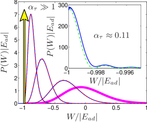
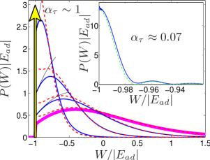
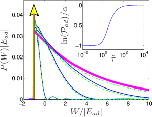
Figure 1: (Color online) The PDF of work done on a LL is plotted after a linear quench from the numerical evaluation of Eq. (13) (blue solid line). Left panel: $\alpha=20$ with $\tilde{\tau}=0$, 1, 2.5 and 5 from right to left and 180 (inset, $P(W>E_{ad})$ only); middle panel: $\alpha=4$ with $\tilde{\tau}=0$, 1, 2 and 4 with increasing peak height and 55 (inset); right panel: $\alpha=0.2$ with $\tilde{\tau}=0$, 2, 5, and 25 from right to left. The thick magenta line denotes the exact SQ expression (Eq. (17)), the red dashed line represent Eq. (21), the thin black line in the middle panel visualizes Eq. (19), while the green dash-dotted line shows Eq. (20). The vertical arrow at $W=E_{ad}$ denotes the Dirac-delta peak, whose spectral weight $\mathcal{P}_{ad}$ is shown in the inset of the right panel on semilog scale as a function of the ramp time $\tau$.

Sudden quench (SQ) limit. In the extreme limit of a SQ, $\tau\ll\tau_{0}$, $G(\lambda,\tau)$ simplifies to $G(\lambda)=\exp\left[{iE_{ad}\lambda^{2}}/{(\lambda+i\tau_{0})}\right]$, and the continuum part of the PDF of work is evaluated exactly as

$$\rho_{\rm SQ}(w)=\mathcal{P}_{ad}\;\exp(-\alpha w)\;{\alpha}\;{w^{-1/2}}\;I_{1}\bigl{(}2\alpha\sqrt{w}\bigr{)}\;,$$ (17)

with $\mathcal{P}_{ad}=\exp(-\alpha)$ and $I_{1}(x)$ the modified Bessel function of the first kind. This is the non-central $\chi^{2}$ distribution with non-centrality parameter $4\alpha$ in the limit of zero degrees of freedom siegel . The average work is zero doraquench , since for a SQ the system remains in its initial state and — on average — there is no back reaction. Entropy is, however, generated by populating high and low energy configurations.

The shape of $\rho(w)$ depends crucially on the orthogonality parameter, $\alpha$. In the thermodynamic limit, $\alpha\gg 1$, almost all probability weight is carried by a peak centered at around $W=0$ ($w=1$) and of width $\Delta W\sim|E_{ad}|/\sqrt{\alpha}$,

$$\rho_{\rm SQ}^{\alpha\gg 1}(w\gg\alpha^{-2})\approx\dfrac{\exp\left(-\alpha\left[1-\sqrt{w}\right]^{2}\right)}{w^{3/4}\sqrt{4\pi\alpha^{-1}}}\;,$$ (18)

whose high energy tail decays according to the Gamma distribution, $\sim\exp(-\alpha w)/w^{3/4}$. In the small system regime $\alpha\ll 1$, on the other hand, the delta function retains almost all weight, and transfers only a fraction $\sim\alpha$ to an exponential distribution of width $\Delta W\sim|E_{ad}|/\alpha$ and threshold at $E_{ad}$ for $w\ll\alpha^{-2}$. In the cross-over regime, $\alpha\sim 1$, the maximum shifts to lower energies and the PDF of work develops a sizable value right above the threshold at $E_{ad}$ (see Fig. 1). The maximum of $P(W)$ occurs at $W>E_{ad}$ for $\alpha>2$, while the PDF becomes monotonically decreasing for $\alpha<2$.

Finite quench times. For finite duration quenches, in addition to the orthogonality parameter $\alpha$, the work statistics also depends on $\tau$ and the protocol $Q(t)$ itself. For definiteness, we focus here on a linear quench EPAPS , and measure the degree of adiabaticity by $\tilde{\tau}=\tau/\tau_{0}$.

For a finite duration quench, $\tilde{\tau}>1$, only a fraction $1/\tilde{\tau}$ of the excitations experiences the quench as sudden. Consequently, in the expression of ${\cal P}_{ad}$, the orthogonality exponent $\alpha$ is replaced by $\alpha_{\tau}\sim\alpha/\tilde{\tau}$, and ${\cal P}_{ad}$ becomes a monotonously increasing function of $\tilde{\tau}$ (see Fig. 1). The crossover with increasing $\alpha_{\tau}$ from $\mathcal{P}_{ad}\lesssim 1$ to vanishingly small spectral weight, $\mathcal{P}_{ad}$, occurs at $\alpha\sim\tilde{\tau}$.

Close to the threshold, $W-E_{ad}\ll 1/\tau$, only states with energy smaller than $1/\tau$ and thus feeling a SQ contribute to work. Therefore, apart from a normalization factor, the PDF of work agrees with the SQ result,

$$\rho(w\ll\alpha^{-1}\tilde{\tau}^{-1})\approx\mathcal{P}_{ad}\exp(\alpha)\rho_{SQ}(w)\;,$$ (19)

and depends on $\tau$ only through $\mathcal{P}_{ad}$.

For $\tilde{\tau}\gg 1$, however, Eq. (19) describes only a small region close to $E_{ad}$ (see thin black lines in Fig. 1), and the overall shape depends both on $\alpha$ and $\tilde{\tau}$. For $4\alpha\gg\tilde{\tau}$, almost all spectral weight is carried by the non-adiabatic processes ($\rho(w)$) around the typical value $W_{typ}-E_{ad}\sim 2|E_{ad}|\ln(\tilde{\tau})/\tilde{\tau}^{2}$, clearly separated from the adiabatic process. For $\tilde{\tau}\gg 4\alpha$, the adiabatic process gains spectral weight, $\mathcal{P}_{ad}\approx 1$, but a maximum for $W>E_{ad}$ remains present, though it gradually merges with the adiabatic processes.

In particular, in the small system limit $\alpha_{\tau}\ll 1$, e.g., we can expand Eq. (13) to get

$$\rho(w)\approx\mathcal{P}_{ad}\alpha^{2}\left(\frac{\sin[w\alpha\tilde{\tau}/2]}{w\alpha\tilde{\tau}/2}\right)^{2}\exp(-\alpha w)\;.$$ (20)

Thus, for a linear quench, for energies commensurate with the quench time the PDF is zero (see Fig. 1). This is related to the steady state behavior of the occupation numbers, $n_{q}\approx[{g_{2}(q)\sin(v|q|\tau)}/{2v^{2}|q|\tau}]^{2}$ for $g_{2}\ll v$ EPAPS , reflecting that modes with energy commensurate to the quench time stay almost unoccupied at $T=0$. In this limit ($\alpha\ll\tilde{\tau}$ and $\tilde{\tau}\gg 1$), the system evolves almost adiabatically, non-adiabatic processes have only a small probability $\sim\alpha/\tilde{\tau}$, and the typical work done in case of a rare non-adiabatic process is $W_{typ}\approx-\alpha^{2}\pi/\tau$.

Increasing $\alpha$, the zeros of the PDF turn gradually into dips, and the PDF develops a more universal form. In the thermodynamic limit $\alpha_{\tau}\gg 1$, using the method of steepest descent we obtain

$$\rho(w)\approx\frac{\mathcal{P}_{ad}\tilde{\tau}^{3/2}\sqrt{\alpha}}{2\sqrt{\tan^{3}(s)\pi}}\exp\left(w\left(\frac{\tilde{\tau}^{2}}{2}-\alpha\right)+2\frac{\alpha s}{\tilde{\tau}}\right)$$ (21)

for $\alpha s\gg\tilde{\tau}$, with $s\equiv\arctan[\sqrt{\exp(w\tilde{\tau}^{2})-1}]$. For $w\gg 1/\tilde{\tau}^{2}\gg 1/\alpha^{2}$, $\rho(w)$ in Eq. (21) behaves as a generalized Gumbel distribution of index $a=\frac{1}{2}+\frac{2\alpha}{\tilde{\tau}^{2}}$ clusel . This latter emerges in the context of global fluctuations, describing the limit distribution of the $a$-th maximum of a sequence of independent and identically distributed random variables gritsev . The distribution in the $1/\tilde{\tau}^{2}\gg w\gg 1/\alpha^{2}$ region resembles closely to Eq. (18) apart from its normalization.

Experimental relevance. Our results can be tested on one-dimensional hard-core bosons kinoshitascience or non-interacting fermions as initial states. The detection of the PDF of work requires two energy measurements, one before and one after the time dependent protocol. The first energy measurement can be omitted if we prepare the initial wave function in an energy eigenstate of $H(t=0)$. The resulting energy distribution can then be probed using time-of-flight experiments polkovnikovrmp ; BlochDalibardZwerger_RMP08 , similarly to Ref.  chen . The crossover between the various regimes can be monitored by tuning $\tau/\tau_{0}$ and $\alpha\sim N\left({g_{2}}/{v}\right)^{2}$, where $N$ is the number of particles in a 1D trap, typically with $N\sim 10^{2}$ - $10^{3}$ atoms paredes ; hofferberth ; kinoshita . By choosing $g_{2}/v\sim 1/\sqrt{N}$, $\alpha$ becomes of order unity, facilitating the observation of crossover between the various regimes. For one-dimensional interacting bosons (i.e. Bose-Hubbard model), $v\sim J$ and $g_{2}\sim J^{2}/U$ for $U\gg J$ (close to the hard-core boson limit) with $U$ the on-site interaction cazalillarmp and $J$ the hopping amplitude. By quenching away from the initial $U\gg J$ $\Leftrightarrow$ $g_{2}\approx 0$ limit (e.g. by changing the lattice parameters or tuning the Feshbach resonance), a final interaction $U\sim J\sqrt{N}$ is reachable. For weakly interacting fermions, $v\sim J$ and $g_{2}\sim U$, therefore ramping from the weakly interacting case to $U\sim J/\sqrt{N}$ is desirable. Nonetheless, our results apply also to interacting initial statesEPAPS .

Summary. We have studied the PDF of work done on a LL after an interaction quench, realizable in strongly interacting Bose systems. We have constructed the density matrix of the generalized Gibbs ensemble with intermode correlations, describing arbitrary correlations of the steady state, thus the PDF of work. The PDF exhibits markedly different characteristics depending on the system size, quench duration and interaction strength. Our method is applicable to the full PDF of other observables as well, e.g. density fluctuations armijo . We also emphasize that our results in Eqs. (11) and (12) apply also to a variety of other systems with effective bosonic Hamiltonians as in Eq. (1), including interacting higher dimensional bosons or spin systems within a spin-wave theory.

I Supplementary material for ”Generalized Gibbs ensemble and work statistics of a quenched Luttinger liquid”

II Quenching between interacting Luttinger liquids

We demonstrate here that our results for the PDF of work applies also when we quench between interacting initial and final states. More precisely, we do not need to start directly from the hard core boson limit for a bosonic LL or from strictly non-interacting fermions for a fermionic LL. Let’s consider an initially interacting LL, given by

$$H_{i}=\sum_{q\neq 0}\omega_{q}b_{q}^{+}b_{q}+\frac{g_{q}^{i}}{2}[b_{q}b_{-q}+b_{q}^{+}b_{-q}^{+}]\;,$$ (S1)

where $g_{q}^{i}$ is the initial interaction. This can conveniently be diagonalized by a standard, time independent Bogoliubov transformation as

$$b_{q}=\cosh(\phi_{q})a_{q}-\sinh(\phi_{q})a_{-q}^{+},$$ (S2)

$$\tanh(2\phi_{q})=\frac{g_{q}^{i}}{\omega_{q}},$$ (S3)

yielding

$$H_{i}=E_{i}+\sum_{q\neq 0}\tilde{\omega}_{q}a_{q}^{+}a_{q},$$ (S4)

where $\tilde{\omega}_{q}=\sqrt{(\omega_{q})^{2}-(g_{q}^{i})^{2}}$, and $E_{i}$ is the ground state energy of $H_{i}$ with respect to the non-interacting ground states. The ground state of this Hamiltonian is the vacuum of the $a$ bosons.

The interaction quench is described, in the language of the initial bosonic operators, by the additional term

$$H^{\prime}=\sum_{q\neq 0}\frac{\Delta g_{q}(t)}{2}[b_{q}b_{-q}+b_{q}^{+}b_{-q}^{+}],$$ (S5)

where $\Delta g_{q}(t)=(g_{q}^{f}-g_{q}^{i})Q(t)$, and $g_{q}^{f}$ is the final interaction strength. After applying Eq. (S2) to this, we obtain the total time dependent Hamiltonian, $H=H_{i}+H^{\prime}$ as

$$H=E_{i}+\sum_{q\neq 0}\left\{\left(\tilde{\omega}_{q}-\frac{\Delta g_{q}(t)}{2}\frac{g_{q}^{i}}{\tilde{\omega}_{q}}\right)a_{q}^{+}a_{q}+\right.$$

$$\left.+\frac{\Delta g_{q}(t)}{2}\frac{\omega_{q}}{\tilde{\omega}_{q}}[a_{q}a_{-q}+a_{q}^{+}a_{-q}^{+}]-\frac{\Delta g_{q}(t)}{2}\frac{g_{q}^{i}}{\tilde{\omega}_{q}}\right\}.$$ (S6)

This, apart from the constant first and last terms on the r.h.s, is identical to Eq. (1) in the main text, after redefining its parameters, $v$, $\delta v$ and $g_{q}(t)$ appropriately. Therefore, our results for the PDF of work apply for any initial and final interactions, provided that we stay in the perturbative regime throughout the quench, namely $\omega_{q}\gg|g_{q}^{i}|,|g_{q}^{f}|$. The threshold above which work is possible, occurs at the difference of the adiabatic ground state energies of the final and initial states, namely at $E_{ad}=-({L/v})[(g_{2}^{f})^{2}-(g_{2}^{i})^{2}]/(v\tau_{0})^{2}16\pi+\dots$. The orthogonality exponent is determined by another energy scale, $E_{oe}=|E_{ad}(g_{2}^{f}-g_{2}^{i})/(g_{2}^{f}+g_{2}^{i})|$, giving $\alpha=E_{oe}\tau_{0}$. After redefining $w=(W-E_{ad})/E_{oe}$, our results for $p(w)$ hold for this general case as well.

III Calculating the characteristic function of work

The Hamiltonian in the Heisenberg picture for $t>\tau$ is given by

$$H_{H}(t)=\sum_{q>0}c_{0}(q,t)\left(b_{q}^{+}b_{q}+b_{-q}b^{+}_{-q}\right)-\omega_{q}(t)+$$

$$+c_{1}(q,t)b_{q}b_{-q}+c_{1}^{*}(q,t)b_{q}^{+}b_{-q}^{+}.$$ (S7)

where

$$c_{0}(q,t)=\omega_{q}(t)\left(|u_{q}(t)|^{2}+|v_{q}(t)|^{2}\right)+$$

$$+g_{q}(t)2\textmd{Re}[u_{q}(t)v_{q}^{*}(t)],$$ (S8)

$$c_{1}(q,t)=2\omega_{q}(t)u_{q}(t)v_{q}(t)+g_{q}(t)(u_{q}^{2}(t)+v_{q}^{2}(t)).$$ (S9)

This is simplified upon realizing that the operators

$$K_{0}(q)=\frac{b^{+}_{q}b_{q}+b_{-q}b^{+}_{-q}}{2},$$ (S10)

$$K_{+}(q)=b^{+}_{q}b^{+}_{-q},\hskip 28.45274ptK_{-}(q)=b_{q}b_{-q}$$ (S11)

are the generators of a SU(1,1) Lie algebra, satisfying $[K_{+}(q),K_{-}(q)]=-2K_{0}(q)$, $[K_{0}(q),K_{\pm}(q)]=\pm K_{\pm}(q)$, and the operators for distinct $q$’s commute with each other. Following Ref. truax , we obtain

$$\exp[i\lambda H_{H}(t)]=\prod_{q>0}\exp[\beta_{+}(q,\lambda,t)K_{+}(q)-i\omega_{q}(t)\lambda]\times$$

$$\times\exp[2\beta_{0}(q,\lambda,t)K_{0}(q)]\exp[\beta_{-}(q,\lambda,t)K_{-}(q)],$$ (S12)

and the $\beta_{\pm,0}(q,\lambda,t)$ coefficients can be determined using Ref. truax . When starting from the ground state at $T=0$, the characteristic function of work is obtained as

$$\tilde{G}(\lambda,\tau)=\exp\left(\sum_{q>0}\beta_{0}(q,\lambda,t)-i\omega_{q}(t)\lambda\right)$$ (S13)

with

$$\beta_{0}(q,\lambda,t)=-\ln\left(\cos(\Omega_{q}\lambda)-\right.$$

$$\left.-i\frac{\omega_{q}(t)+2\textmd{Im}[v_{q}^{*}(t)\partial_{t}v_{q}(t)]}{\Omega_{q}}\sin(\Omega_{q}\lambda)\right),$$ (S14)

where $\Omega_{q}=\sqrt{\omega_{q}^{2}(t>\tau)-g_{q}^{2}(t>\tau)}$ is the time independent adiabatic eigenenergy of a given mode in the final LL stategiamarchi . After some trivial steps, Eq. (S13) is rewritten as

$$\ln\left(\tilde{G}(\lambda,\tau)\right)=-\sum_{q>0}\ln\left(1+n_{q}(1-\exp[2i\Omega_{q}\lambda])\right)+$$

$$+i\lambda E_{ad},$$ (S15)

where

$$n_{q}=\frac{\omega_{q}(t)+2\textmd{Im}[v_{q}^{*}(t)\partial_{t}v_{q}(t)]}{2\Omega_{q}}-\frac{1}{2}$$ (S16)

is the occupation number in the steady state and

$$E_{ad}=\sum_{q>0}\left[\Omega_{q}-\omega_{q}(t>\tau)\right].$$ (S17)

is time independent, and stands for the difference of the adiabatic ground state energies of the final and initial states.

The occupation number in the steady state is obtained for a linear quench from Eq. (S16) using the results of Ref. doraquench as

$$n_{q}\approx\left[\frac{g_{2}(q)\sin(v|q|\tau)}{2v^{2}|q|\tau}\right]^{2}$$ (S18)

for $g_{2}\ll v$. We have checked this prediction by numerically solving the differential equation in Eq. (3) in the main text. The occupation numbers turn out to be periodic in the time averaged mode energies, defined by

$$\omega_{av}(q)=\frac{1}{\tau}\int\limits_{0}^{\tau}\sqrt{\omega_{q}^{2}(t)-g_{q}^{2}(t)}dt,$$ (S19)

and the numerically evaluated occupation numbers are plotted in Fig. S1. States with average energy commensurate with $\tau$ possess the lowest effective temperatures. The zeros predicted by Eq. (S18) turn to sharp dips with increasing interaction, and our analytical expression describes rather reliably the numerical data. Although for finite $g_{2}$, all effective temperatures are finite, the steady state is far from being thermal, as evidenced by the highly non-thermal structure of the steady state density matrix.

\psfrag{x}[t][1][0]{$\omega_{av}(q)\tau/2\pi$}\psfrag{y}[b][t][1][0]{$(v/g_{2})^{2}n_{q}$}\includegraphics[width=156.49014pt]{nqexact.eps}

Figure S1: The numerically evaluated occupation numbers in the steady state are plotted on a semilogarithmic scale after a linear quench with $\delta v=0$, $g_{2}/v=0.1$ (blue solid line), 0.5 (red dashed line) and 0.8 (black dash-dotted line), ranging from weak to strong interactions. The result of Eq. (S18) is practically indistinguishable from the blue solid curve except close to $\omega_{av}(q)=2\pi n/\tau$ with $n$ integer, where the effective temperatures are the lowest. The figure is valid for arbitrary $q$ since it depends only on the dimensionless combination $\omega_{av}(q)\tau$.

IV On the steady state density matrix from GGE

The steady state density matrix reveals a highly non-thermal structure, namely

$$\hat{\rho}_{G}=\frac{1}{Z_{G}}\prod_{q>0}\exp\left[-\beta_{q}\Omega_{q}\hat{n}_{q}\right]\delta_{\hat{n}_{q},\hat{n}_{-q}},$$ (S20)

possessing finite matrix elements only along $\hat{n}_{q}=\hat{n}_{-q}$. Thermalization would mean the same matrix elements for a fixed $\hat{n}_{q}+\hat{n}_{-q}$, which is not the case here. Therefore, one can ask to what extent this density matrix is immune to additional perturbations, not considered within our Hamiltonian.

On the one hand, one can argue that experimental results on one dimensional cold atoms did not find any sign of thermalization, but rather prethermalization, i.e. reaching a certain non-thermal steady state, took placekinoshita ; gring ; hofferberth ; hofferberthnatphys . These experimental results are nicely accounted for by a simple Gaussian model, similar to our Eq. (1) in the main text, without additional terms. On the other hand, from a theoretical point of view, additional interactions between the $b$ bosons are generated by the non-linearity of the non-interacting dispersion relation. As was investigated in Ref. samokhin ; imambekovrmp , this broadens the otherwise sharp peak around the bare dispersion at $\omega_{q}=v|q|$ in the spectral function of the bosons, which, as a rough estimate, scales with $\sim q^{2}/m$, where $m$ is the effective mass arising from curvature effects. In the long wavelength limit ($q\sim 0$), this gives a ”lifetime”, which is usually much longer that the typical experimental timescales. Higher order terms in the $b$ bosons also arise from density-density interactionscazalillarmp , but these provide higher powers of $q$ in the broadening of the bosonic mode, suppressing further their effect.

Nonlinear terms of sine-Gordon type giamarchi are absent without any lattice, i.e. for interacting particles in the continuum limit, which can also be realized experimentallykinoshitascience . In the presence of an optical lattice, these are inevitably present, though their effect can be weakened by choosing incommensurate fillings or suppressing spin backscattering (e.g. by using single component bosons). Therefore, our non-thermal density matrix in Eq. (S20) is expected to describe fairly reliably the steady state of interaction quenched one dimensional systems.

Having established the validity of our density matrix, we now turn to the derivation of results, presented in the main text, using the steady state density matrix. The partition function of the GGE is determined as

$$Z_{G}=\prod_{q>0}\frac{1}{1-\exp[-\beta_{q}\Omega_{q}]},$$ (S21)

and the characteristic function of work reads as

$$\tilde{G}(\lambda,\tau)\exp(-i\lambda E_{ad})=$$

$$=\frac{1}{Z_{G}}\prod_{q>0}\sum\limits_{n_{q}=0}^{\infty}\exp\left[-\beta_{q}\Omega_{q}+2i\lambda\Omega_{q}n_{q}\right]=$$

$$=\prod_{q>0}\frac{1-\exp[-\beta_{q}\Omega_{q}]}{1-\exp[-\beta_{q}\Omega_{q}+2i\lambda\Omega_{q}]}=$$

$$=\exp\left(-\sum_{q>0}\ln\left(\frac{\exp[\beta_{q}\Omega_{q}]-\exp[2i\lambda\Omega_{q}]}{\exp[\beta_{q}\Omega_{q}]-1}\right)\right)=$$

$$=\exp\left(-\sum_{q>0}\ln\left(1+\frac{1-\exp[2i\Omega_{q}\lambda]}{\exp(\beta_{q}\Omega_{q})-1}\right)\right).$$ (S22)

V The cumulants of energy

The cumulants, $C_{n}$ of the PDF of work done can be derived after expanding the characteristic function of work done in power series as $\ln\left(\tilde{G}(\lambda,\tau)\right)=\sum_{n=1}^{\infty}C_{n}(i\lambda)^{n}/n!$, yielding

$$\frac{C_{n}}{E_{ad}}=\delta_{n,1}-\int\limits_{0}^{\tau}\int\limits_{0}^{\tau}\frac{Q^{\prime}(t_{1})Q^{\prime}(t_{2})\tau_{0}^{2}n!}{\left[i(t_{1}-t_{2})-\tau_{0}\right]^{n+1}}dt_{1}dt_{2},$$ (S23)

where the first term denotes the adiabatic ground state energy difference between the initial and final state, while the second one stems from the non-adiabatic evolution (i.e. heat). The first cumulant, $C_{1}=\langle H(t>\tau)\rangle$ was already calculated in Ref. doraquench, . Their behaviour is illustrated in Fig. S2 after a linear quench: $C_{1}-E_{ad}$ decays as $\ln(\tau/\tau_{0})/\tau^{2}$, since $Q^{\prime}(t)$ exhibits kinks at $t=0$ and $\tau$doraquench ; degrandi , consequently all $C_{n>1}$ decay as $\tau^{-2}$.

For a SQ, the cumulants are $C_{1}=\langle H(t>0)\rangle=E_{SQ}(=0$ to second order in $g_{2}$ and $\delta v$ within our scheme), $C_{n>1}=\alpha n!/\tau_{0}^{n-2}$.

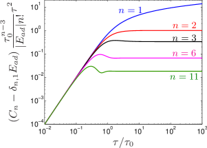
Figure S2: (Color online) Several cumulants of the work done on a LL are log-log plotted as a function of the quench time for a linear protocol. Close to the SQ limit ($\tau\ll\tau_{0}$), all properly normalized cumulants are equal, while in the near adiabatic limit ($\tau\gg\tau_{0}$), these approach $2/n(n-1)$.

VI Analytical results for a linear quench

In the case of a linear quench, the characteristic function of work is obtained as

$$\ln\left[\tilde{G}(\lambda,\tau)\right]=iE_{ad}\left[\lambda-\frac{\tau_{0}^{2}}{\tau^{2}}\left(g(\lambda+i\tau_{0})-g(i\tau_{0})\right)\right],$$ (S24)

where $g(z)=(z+\tau)\ln(z+\tau)+(z-\tau)\ln(z-\tau)-2z\ln(z)$. The cumulants are obtained from a variant of Eq. (S23) as

$$\frac{C_{n}}{E_{ad}}=\delta_{n,1}-{(-1)^{n}\tau_{0}^{2}}\frac{\partial^{n-1}}{\partial\tau_{0}^{n-1}}\frac{\Delta E}{E_{ad}\tau_{0}^{2}},$$ (S25)

where the heating, $\Delta E$ is

$$\Delta E=-E_{ad}\frac{\tau_{0}^{2}}{\tau^{2}}\ln\left(1+\frac{\tau^{2}}{\tau_{0}^{2}}\right),$$ (S26)

and Eq. (S25) holds true for an arbitrary quench protocol. The asymptotic behaviour of Eq. (S24) for $\lambda\rightarrow\infty$ gives

$$\tilde{G}(\lambda\rightarrow\infty,\tau)=\exp\left(i\lambda E_{ad}-2\frac{\alpha}{\tilde{\tau}}\arctan\left(\tilde{\tau}\right)\right)\times$$

$$\times\left(1+\tilde{\tau}^{2}\right)^{\alpha/\tilde{\tau}^{2}}=\left\{\begin{array}[]{cc}\exp\left(i\lambda E_{ad}-\dfrac{\pi\alpha}{\tilde{\tau}}\right)&\tau\rightarrow\infty,\\ \exp\left(i\lambda E_{ad}-\alpha\right)&\tau\rightarrow 0.\end{array}\right.$$ (S29)

From this, the asymptotic behaviour of $P_{ad}$ follows as

$$P_{ad}=\left\{\begin{array}[]{cc}\exp\left(-\alpha+\dfrac{\alpha\tilde{\tau}^{2}}{6}\right),&\tau\rightarrow 0,\\ 1-\dfrac{\pi\alpha}{\tilde{\tau}},&\tau\rightarrow\infty.\end{array}\right.$$ (S32)