Numerical approximation of one phase quadrature domains

Abstract.

In this work, we present two numerical schemes for a free boundary problem called one phase quadrature domain. In the first method by applying the proprieties of given free boundary problem, we derive a method that leads to a fast iterative solver. The iteration procedure is adapted in order to work in the case when topology changes. The second method is based on shape reconstruction to establish an efficient Shape-Quasi-Newton-Method. Various numerical experiments confirm the efficiency of the derived numerical methods.

1. Introduction.

In this paper we shall consider general mathematical approaches to solve the free boundary problems of type

(1.1) $$A(u,\Omega)=0,$$

(1.2) $$B(u,\Omega)=0.$$

Here $A$ corresponds to a well posed elliptic boundary value problem in an unknown domain $\Omega=\{x\,:\,u(x)>0\}=\{u>0\}$ and $B$ operates on the functions supported at the free boundary $\Gamma=\partial\Omega$. It is supposed that function $u$ can be solved from equation (1.1) for any given suitable domain $\Omega.$ More precisely, in this paper we consider the following problem:

(P) $$\begin{cases}\Delta u=\chi_{\Omega}-\mu,&\mbox{in}\quad\,\,\mathbb{R}^{N},\\ u\geq 0,&\mbox{in}\quad\mathbb{R}^{N},\\ u=0,&\mbox{in}\quad\mathbb{R}^{N}\setminus\Omega,\end{cases}$$

where $\mu$ is a given measure with compact support. Our aim in this work is to study systematic and efficient ways to solve Problem (P) numerically. The outline of the paper is as follows.

In section 2, we present some basic facts and mathematical background of quadrature domains. In section 3, we investigate one of the applications of quadrature domains, Hele Shaw flow. Section 4 is devoted to derive a numerical scheme which is based on the properties of the free boundary especially blow up techniques. In section 5 we construct another numerical scheme for Problem (P) based on shape reconstruction formulation. Finally, in last section we investigate some numerical examples which show the efficency of the numerical algorithms.

2. Notations and mathematical background of quadrature domains.

Let us review some notations that we use here. By $\Omega$ we mean an open subset of $\mathbb{R}^{N}$ and $L^{p}(\Omega)$ the usual Lebesgue space with respect to the Lebesgue measure. $HL^{p}(\Omega)$ denote the subspace of $L^{p}(\Omega)$ that consists of harmonic functions and $SL^{p}(\Omega)$ for the subspace of $L^{p}(\Omega)$ that consists of subharmonic functions. We also show the characteristic function of $\Omega$ by $\chi_{\Omega}$ and $G$ always denotes the usual ”fundamental solution” for the Laplace operator in $\mathbb{R}^{N}$. In other words, for $x\in\mathbb{R}^{N}\setminus\{0\}$

$$G(x)=\begin{cases}\frac{1}{N(N-2)\omega_{N}}|x|^{2-N},&{\rm for~{}~{}~{}}N\geq 3,\\ -\frac{1}{2\pi}\ln|x|,&{\rm for~{}~{}~{}}N=2,\end{cases}$$

where $\omega_{N}$ denotes the volume of the unit ball in $\mathbb{R}^{N}$.

It is immediately verified that if $\Omega$ is open and bounded then as function of $x\in\Omega$,

$$G(x-y)\in HL^{1}(\Omega),\quad\,\,\text{for all }y\in\Omega^{c},$$

$$-G(x-y)\in SL^{1}(\Omega),\quad\,\,\text{for all }y\in\Omega.$$

Definition 2.1.

Let $\mu$ be a measure with compact support. By a subharmonic quadrature domain we mean an open connected set $\Omega\subset\mathbb{R}^{N}$ such that $supp(\mu)\subset\Omega$ and

(2.1) $$\int_{\Omega}h\,dx\geq\int\,h\,d\mu,$$

holds for all $h\in SL^{1}(\Omega)$. We write $\Omega\in Q(\mu,SL^{1})$ if (2.1) holds and $\mu(\Omega)<\infty$.

If one consider $\int_{\Omega}h\,dx=\int\,h\,d\mu$ for all $h\in HL^{1}(\Omega)$ then $\Omega$ is a quadrature domain and we write $\Omega\in Q(\mu,HL^{1})$.

The simplest quadrature domain is a circular disc. Suppose that $\mu=\alpha\delta_{0}$ where $\delta_{0}$ is a Dirac mass at origin and $\alpha>0$. Then

$$Q(\mu,HL^{1})=Q(\mu,SL^{1})=\{B(0;r)\},$$

where $r\geq 0$ is determined by $|B(0;r)|=\alpha$, (see [6]). Generally if $\Omega$ is a bounded domain in $\mathbb{R}^{N}$ and

(2.2) $$\int_{\Omega}~{}hdx=|\Omega|\,h(x_{0}),$$

holds for all $h\in HL^{1}(\Omega)$, where $x_{0}$ is an arbitrary point, then $\Omega$ is a ball centered at $x_{0}$.

In this article we deal only with subharmonic quadrature domain, and from now on by a quadrature domain we mean a subharmonic quadrature domain.

Let $U^{\mu}$, the Newtonian potential of the measure $\mu$ which is defined by

$$U^{\mu}(x):=(G*\mu)(x)=\int_{\mathbb{R}^{N}}G(x-y)d\mu(y),~{}~{}~{}x\in\mathbb{R}^{N},$$

and it satisfies the Poisson’s equation $-\Delta U^{\mu}=\mu$ in the distribution sense. For the sake of simplicity, we shall use $U^{\Omega}$ instead of $U^{\chi_{\Omega}}$.

Gustafsson in [6] has showed that $\Omega\in Q(\mu,SL^{1})$ if and only if

(2.3) $$\begin{cases}U^{\Omega}\leq U^{\mu},&\hbox{in}\,\mathbb{R}^{N},\\ U^{\Omega}=U^{\mu},&\hbox{in}\,\mathbb{R}^{N}\setminus\Omega.\end{cases}$$

Also if one considers $u=U^{\mu}-U^{\Omega}\geq 0$, then

(2.4) $$\Delta u=\chi_{\Omega}-\mu\quad\mbox{in}\quad\mathbb{R}^{N}.$$

Note that from (2.4) one has $\Delta u=\chi_{\Omega}$ away from $supp(\mu)$ and according to the results in local regularity of solutions for elliptic PDEs, we obtain $u\in W_{\text{loc}}^{2,p}(\mathbb{R}^{N})$, for every $1<p<\infty$. Also $\nabla u\in W_{\text{loc}}^{1,p}(\mathbb{R}^{N})$. By the Sobolev embedding theorem the first derivatives are therefore Hölder continuous with Hölder exponent $\alpha<1$.

Sakai in [13] has proved that the definition of quadrature domain is equivalent to the well-known one-phase free boundary problem in distribution scenes. More precisely, from PDE point of view, $\Omega\in Q(\mu,SL^{1})$ is equivalent to

(2.5) $$\begin{cases}\Delta u=\chi_{\Omega}-\mu,&\mbox{in}\quad\mathbb{R}^{N},\\ u\geq 0,&\mbox{in}\quad\mathbb{R}^{N},\\ u=0,&\mbox{in}\quad\mathbb{R}^{N}\setminus\Omega.\end{cases}$$

Remark 1.

Suppose that $m$ denotes the Lebesgue measure. By (2.3) we know that $u=|\nabla u|=0$ in $\mathbb{R}^{N}\setminus\Omega$. Now taking integration of (2.4) gives

$$0=\int_{\partial\Omega}\frac{\partial u}{\partial n}\,ds=\int_{\Omega}\Delta u\,dx\,=\,m(\Omega)-\mu(supp(\mu)).$$

This fact is also a consequence of (2.1). In other words, we know the volume of the solution priori.

Example 2.2.

As an other example of one phase quadrature domain, suppose that $x_{0}\in\mathbb{R}^{N}$ and $a>0,\,M>1$. Let $B_{1}=B_{1}(x_{0},a)$ and $\mu=M\chi_{B_{1}}$. Then (2.5) reads

(2.6) $$\begin{cases}\Delta u=\chi_{\Omega}-M\chi_{B_{1}},&\mbox{in}\,\,\Omega,\\ u=|\nabla u|=0,&\mbox{in}\,\,\Omega^{c}.\end{cases}$$

The spherical symmetry of the problem shows that the we have to find a radial solution $u=u(|x|)$ for (2.6). Consequently, we suppose that $\Omega=B_{2}=B_{2}(x_{0},r)$ for some $r>a$. To make more easier we consider that $u=u_{1}$ on $B_{1}$ and $u=u_{2}$ on $B_{2}\setminus B_{1}$. We desire to patch $u_{1}$ and $u_{2}$ on $\partial B_{1}$ without loosing regularity. Therefore our problem is

(2.7) $$\Delta u=\begin{cases}1-M,&\mbox{in}~{}~{}B_{1},\\ 1,&\mbox{in}~{}~{}B_{2}\setminus B_{1},\end{cases}$$

with the following conditions

(2.8) $$\begin{cases}u_{1}=u_{2},\,\,\nabla u_{1}=\nabla u_{2},&\mbox{in}~{}~{}B_{1},\\ u_{2}=|\nabla u_{2}|=0&\mbox{in}~{}~{}(B_{2})^{c}.\end{cases}$$

By some calculations and considering the fundamental solution for Laplacian operator one has

(2.9) $$u(x)=\begin{cases}(1-M)\frac{|x-x_{0}|^{2}}{2N}+A_{1},&\mbox{in}~{}~{}B_{1},\\ \frac{|x-x_{0}|^{2}}{2N}+A_{2}|x-x_{0}|^{2-N}+A_{3},&\mbox{in}~{}~{}B_{2}\setminus B_{1},\\ 0,&\mbox{in}~{}~{}(B_{2})^{c},\end{cases}$$

where $A_{1},A_{2},A_{3}$ are appropriate constants which are computed with respect to (2.8). Now we obtain

(2.10) $$u(x)=\begin{cases}(1-M)\frac{|x-x_{0}|^{2}}{2N}+\frac{r^{2}-Ma}{2(2-N)},&\mbox{in}~{}~{}B_{1},\\ \frac{|x-x_{0}|^{2}}{2N}-\frac{r^{N}|x-x_{0}|^{2-N}}{N(N-2)}+\frac{r^{2}}{2(2-N)},&\mbox{in}~{}~{}B_{2}\setminus B_{1},\\ 0,&\mbox{in}~{}~{}(B_{2})^{c},\end{cases}$$

where $r=M^{\frac{1}{N}}a$.

For $N=2$ we can replace $|x-x|^{2-N}$ by $\log|x-x_{0}|$ in (2.10) and we derive that

(2.11) $$u(x)=\begin{cases}(1-M)\frac{|x-x_{0}|^{2}}{4}+\frac{a^{2}}{4}M+\frac{r^{2}}{2}(\log\frac{a}{r}-\frac{1}{2}\big{)},&\mbox{in}~{}~{}B_{1},\\ \frac{|x-x_{0}|^{2}}{4}+\frac{r^{2}}{2}\log|x-x_{0}|-\frac{r^{2}}{2}\big{(}\log r+\frac{1}{2}\big{)},&\mbox{in}~{}~{}B_{2}\setminus B_{1},\\ 0,&\mbox{in}~{}~{}(B_{2})^{c},\end{cases}$$

with $r=M^{\frac{1}{2}}a$.

Remark 2.

Suppose that $N=2,\,\mu=\delta_{0}$. Let $B(0,\epsilon)$ be an approximation of $supp(\mu)$ with $M=\frac{1}{\pi\epsilon^{2}}$ for $\epsilon$ small enough. Then one can obtain $r=\frac{1}{\sqrt{\pi}}$.

2.1. An estimate of quadrature domain.

In Problem (P) the domain $\Omega$ is part of the solution and in order to generate a mesh, one needs to find a domain which contains $\Omega$. To do this we find a bigger domain such that $\Omega$ is embedded in it as follows.

By $r(\mu)$ we mean a positive number corresponding to the positive measure $\mu$ such that

$$|B_{r(\mu)}|=m(B_{r(\mu)})=\int_{\mathbb{R}^{N}}\,d\mu=\mu(\mathbb{R}^{N}),$$

where $m$ denotes the Lebesgue measure in $\mathbb{R}^{N}$. The following theorem is due to Sakai, see [14].

Theorem 2.3.

[14] Let $\mu$ be a finite positive measure with support in the closed ball $\overline{B_{R}},\,R>0$. Then every quadrature domain $\Omega$ of $\mu$ for subharmonic functions satisfies

(2.12) $$\Omega\subset B_{r(\mu)+R}.$$

Furthermore, if $r(\mu)>2R$ then

$$B_{r(\mu)-R}\subset\Omega.$$

For instance let $\mu=g(x)\chi_{B_{1}}$, where $g$ is a positive function with $M=\sup_{B_{1}}g(x)$, then $\Omega\subset B_{\sqrt{M}+1}$.

For more information about one phase quadrature domain see [6, 7, 8, 13, 15].

3. An application (Hele Shaw flow).

One application of Problem (P) appears in Laplacian growth like Hele-Shaw flow which comes up in flow’s dynamic. Here we describe the Hele-Shaw problem briefly.

Suppose that some incompressible fluid has been confined between two parallel plate and we inject more fluid by moderate velocity to it. Therefore the fluid between plates begin to occupy more space. We are interested in to study the behavior of the boundary of the fill space.

To be precise, let $\nu$ be a positive, finite and non zero measure with compact support and $supp(\nu)\subseteq D$ where $D$ is an open subset of $\mathbb{R}^{N}$ by a $C^{1}$ boundary. Let $p_{D}$ be a super harmonic function such that

(3.1) $$\begin{cases}-\Delta p_{D}=\nu&\hbox{in}\,D,\\ p_{D}=0&\hbox{on}\,\partial D.\end{cases}$$

We are looking for a family of regions $D_{t}$ for $t\geq 0$, such that $\partial D_{t}$ moves with the velocity $-\nabla p_{D_{t}}$. This problem was introduced by S. Richardson [12].

Definition 3.1.

Suppose that $I$ is an interval in $\mathbb{R}$. Let $\mu=\chi_{D_{0}}+t\nu$, $t\in I$. A map $t\rightarrow D_{t}\subset\mathbb{R}^{N}$ is a weak solution of the free boundary problem if the function $u_{t}\in H^{1}{(\mathbb{R}^{N})}$ defined by

(3.2) $$\Delta u_{t}=\chi_{D_{t}}-\mu,$$

satisfies the following conditions:

• $u_{t}\geq 0,$

• $\int u_{t}(1-\chi_{D_{t}})\,dx=0.$

Last condition guarantee that $u_{t}=0$ in $\mathbb{R}^{N}\setminus D_{t}$, see [5].

Remark 3.

PDE (3.2) together with the above conditions are a special case of Problem (P).

Next theorem states the corresponding quadrature domain of the solution of the Hele-Shaw problem.

Theorem 3.2.

[5] Suppose that $\mu$ and $D_{0}$ are as before and $T>0$. Then there exists a weak solution

$$[0,T]\ni t\rightarrow D_{t}\subset\mathbb{R}^{N},$$

for Hele Shaw problem which is unique and if $u_{t}$ be the function appearing in (3.2), then $u_{t}$ is also unique and

$$u_{t}=\int_{0}^{t}p_{D_{\tau}}\,d\tau.$$

Moreover, $D_{t}$ can be chosen to be

$$D_{t}=D_{0}\cup\{z:u_{t}(z)>0\}.$$

For more information about Hele shaw see [5], [12], [9] and references therein.

4. First numerical method to approximate the solution of Problem (P).

In this part by applying the properties of free boundary problem, we construct an algorithm that leads us to a fast iterative solver. The level set method is next employed to evolve the interface in the direction of the normal velocity field.

Consider Problem (P) in dimension one. Our motivation for the first method is based on the fact that for any $x$ outside of the $\mbox{supp}(\mu)$ one has

$$u^{\prime}(x)=\pm\sqrt{2u}.$$

To be more precise, one has

(4.1) $$\Delta u=1,\quad\text{in}\,\,{\{x:u(x)>0}\}\setminus supp(\mu).$$

Let $x_{f}$ be a free boundary point. Multiply (4.1) by $u^{\prime}$ and integrate over $[x\,,\,x_{f}]$ to find that

$$\frac{1}{2}(u^{\prime})^{2}(x)=u(x).$$

Let $(c,d)$ be an initial guess for ${\{x:u(x)>0}\}$ which contains the support of measure $\mu$. Next we solve the following boundary value problem

(4.2) $$\begin{cases}u^{\prime\prime}=1-\mu&\mbox{in}\quad(c,d),\\ u^{\prime}(c)=\sqrt{2u(c)},&u^{\prime}(d)=-\sqrt{2u(d)}.\end{cases}$$

Then to get the free boundary points, we move the points $c,d$ in the normal direction with speeds $\sqrt{2u(c)}$ and $\sqrt{2u(d)}$, i.e,

$$d_{f}=d+\sqrt{2u(d)},\quad c_{f}=c-\sqrt{2u(c)},$$

where $c_{f}$ and $d_{f}$ are free boundary points. Note that in this case we need only one iteration, see section 4.2.

Remark 4.

To have existence for the boundary value problem (4.2) one has to choose $(c,d)$ close enough to $\text{supp}(\mu)$.

4.1. Blow up techniques and the main idea.

In higher dimensions we shall prove that when we approach to the free boundary still the quotient $\frac{|\nabla u(x)|}{\sqrt{2u(x)}}$ goes to one. First, we recall some known properties and lemmas that have been proved in [11]. We shall use them in the proof of Theorem 4.6. The following lemma shows the growth of $u$ away from the free boundary $\Gamma$.

Lemma 4.1.

[11] Let $u\in L^{\infty}_{\text{loc}}(\Omega)$, $\Omega={\{u>0}\}$ be a solution of Problem (P). If $\,x_{0}\in\Gamma$ then

$$\underset{B_{r}(x_{0})}{\sup}u\leq Cr^{2},$$

where $C=C(N)$.

Corollary 4.2.

Let $u$ be as in Lemma 4.1. Then

$$u(x)\leq Cdist(x,\partial\Omega)^{2}.$$

Also we need the following Non degeneracy property of the solutions.

Lemma 4.3.

[11] Let $u$ be a solution of given free boundary problem, then we have the inequality

$$\underset{\partial B_{r}(x_{0})}{\sup}\,u\geq\frac{r^{2}}{8N},\quad\,\,\,\,\,\,\text{for any }x_{0}\in\Gamma.$$

Definition 4.4.

(Local solutions) For given $R,M>0,$ and $x_{0}\in\Gamma,$ let $P_{R}(x_{0},M)$ be the class of $C^{1,1}$ solutions $u$ of Problem (P) in $B_{R}(x_{0})$ such that

$$|Du(x)-Du(y)|\leq M|x-y|,\qquad\text{for any }x,y\in\mathbb{R}^{N}.$$

In the case $x_{0}=0$ we also set $P_{R}(M)=P_{R}(0,M).$

In the above definition if $R=\infty$ then we get solutions in the entire space $\mathbb{R}^{N}$ and grow quadratically at infinity, which are called global solutions.

If $u\in P_{R}(x_{0},M)$ and $\lambda>0,$ then the proper re-scaling of $u$ at $x_{0}$ is defined by

$$u_{x_{0},\lambda}(x)=\frac{u(x_{0}+\lambda x)-u(x_{0})}{\lambda^{2}}.$$

Note that by using non degeneracy, Lemma 4.3, and quadratic growth properties, Lemma 4.1, it can be shown that when $\lambda\rightarrow 0$ then

$$u_{x_{0},\lambda}\rightarrow u_{0}\quad\mbox{in}\,\,C_{\text{loc}}^{1,\alpha}(\mathbb{R}^{N})\,\,\mbox{for any}\,\,0<\alpha<1,$$

where $u_{0}\in C_{\text{loc}}^{1,1}(\mathbb{R}^{N})$. This $u_{0}$ is called a blow up of $u$ with fixed center $x_{0}$ and also $u_{0}$ is a global solution, i.e, $u_{0}\in P_{\infty}(M).$ For more details see [11].

Theorem 4.5.

[11] (Blow up with fixed center). Let $u\in P_{R}(x_{0},M)$ be a solution of Problem (P). Suppose that

$$u_{0}(x)=\lim_{j\rightarrow\infty}u_{x_{0},\lambda_{j}}(x),\quad x\in\mathbb{R}^{N},$$

for some sequence $\lambda_{j}\rightarrow 0$ as $j\rightarrow\infty.$ Then $u_{0}$ is homogeneous of degree two with respect to the origin, i.e.

$$u_{0}(\lambda x)=\lambda^{2}u_{0}(x),\quad\text{ for any }x\in\mathbb{R}^{N}\text{ and }\lambda>0.$$

In the proof of next theorem we will use the concept of regular points. A $x_{0}\in\Gamma$ is a regular point if every blow up of $u$ at $x_{0}$ is a half plane solution. Precisely, there is two category of blowup for a solution of the Problem (P). Let $u_{0}$ be a blowup with a fixed center then it has one of the following forms (see [11]):

• Polynomial solution: $u_{0}(x)=\frac{1}{2}(x\cdot Ax),\,x\in\mathbb{R}^{N}.$ Here $A$ is an $n\times n$ symmetric matrix with $Tr(A)=1.$

• Half plane solutions: $u_{0}(x)=\frac{1}{2}(x\cdot e)^{2}_{+},\,x\in\mathbb{R}^{N}$ where $e$ is a unit vector.

Theorem 4.6.

Let $x_{0}$ be a free boundary point and $x\in{\{u>0\}}$ then

$$\limsup_{x\rightarrow x_{0}}=\liminf_{x\rightarrow x_{0}}\frac{|\nabla u(x)|}{\sqrt{2u(x)}}=1.$$

Proof.

By Theorem 4.5, blowup solutions at fixed point $x_{0}\in\Gamma$ is a global homogeneous solution of degree two. Let $u$ be a homogeneous global solution. Then by above discussion, $u$ has the following form

$$u_{0}(x)=\frac{1}{2}(x\cdot e)^{2}_{+},\,x\in\mathbb{R}^{N}\,\,\mbox{where}\,\,e\,\,\mbox{is a unit vector.}$$

Without loss of generality assume that $x_{0}=0$ then we know that

$\frac{u(rx)}{r^{2}}\rightarrow\frac{(x_{1})_{+}^{2}}{2}$ in $C^{1,\alpha},$

which means

$${\left|\frac{u(rx)}{r^{2}}-\frac{(x_{1})_{+}^{2}}{2}\right|}\rightarrow 0,$$

and consequently,

$${\left|\frac{\nabla u(rx)}{r}-x_{1}e_{1}\right|}\rightarrow 0.$$

From above one can get

$$u(rx)=\frac{(rx_{1})_{+}^{2}}{2}+cr^{2},\text{ where }c\text{ is an arbitrary small constant and}$$

$$\nabla u(rx)=(rx_{1})e_{1}+O(r^{\alpha}),\quad\alpha<1.$$

Using above expression for $u(rx)$ and $|\nabla u(rx)|$ and taking the quotient implies the limit. ∎

4.2. A mixed boundary value problem and first algorithm.

Assume $(\Omega,u)$ be a smooth solution of Problem (P). Our aim is to build a sequence $(\Omega_{k},u_{k})$ of solutions of an approximate quadrature domain problem which converges towards $(\Omega,u).$ Assume that $p_{k}\in\partial\Omega_{k}$. Let $\mathbf{n}_{k}$ be the normal outward vector on $\partial\Omega_{k}$. By Taylor formula, one can write

$$u(p_{k}+d_{k}\mathbf{n}_{k})\simeq u(p_{k})+d_{k}\nabla u(p_{k})\cdot\mathbf{n}_{k}+\frac{d_{k}^{2}}{2}\,\mathbf{n}_{k}^{T}\cdot D^{2}u(p_{k})\cdot\mathbf{n}_{k}.$$

We wish to have $u(p_{k}+\mathbf{n}_{k}d_{k})=0$, so if we put $\nabla u(p_{k})\cdot\mathbf{n}_{k}=-\sqrt{2u(p_{k})}$ and use the approximation $D^{2}u\simeq\frac{1}{2}(\Delta u)I$, then one gets

(4.3) $$d_{k}=\zeta\sqrt{2u(p_{k})},$$

where $\zeta=2-\sqrt{2}$. It means that if $\Gamma_{k}=\partial\Omega_{k}$ then $\{\Gamma_{k}+d_{k}\cdot\mathbf{n}_{k}\}$ converges to $\Gamma$. We note that in dimension one, $d_{k}=\sqrt{2u(p_{k})}$.

To construct an algorithm, let $\Omega_{0}$ be an initial guess of $\Omega$ which contains $supp(\mu)$. Consider the following boundary value problem which has a vital role in the numerical scheme

(4.4) $$\begin{cases}\Delta u=1-\mu,&\mbox{ in }\Omega_{0},\\ \frac{\partial u}{\partial n}=-\sqrt{2u},&\mbox{ on }\partial\Omega_{0}.\end{cases}$$

Remark 5.

We note that (4.4) is not stable at the points close to the free boundary, therefore alternatively we solve the following problem to have more efficient and robust scheme,

(4.5) $$\begin{cases}\Delta u_{k}=1-\mu,&\mbox{ in }\Omega_{k},\\ \frac{\partial u_{k}}{\partial n_{k}}=-\theta u_{k},&\mbox{ on }\partial\Omega_{k}.\end{cases}$$

We desire that $\theta u_{k}$ behaves like $\sqrt{2u_{k}}$, therefore one is able to choose

(4.6) $$\theta=\bigg{(}{\frac{2}{\displaystyle\sup_{\partial\Omega_{k-1}}u_{k-1}}}\bigg{)}^{1/2}.$$

To determine an optimal value for $\theta$ we employe the fixed point process and iterate $\theta$ as follows.

First of all, let $\theta$ be as in (4.6) and solve (4.5) to obtain the value of $u$ on $\partial\Omega_{k}$. Then compute the corresponding $\theta$ by the formula (4.6) and repeat the same process again. This scenario will converge to the best choice of $\theta$.

The existence of (4.5) is based on minimization techniques and is a special case of the next lemma.

Lemma 4.7.

[3] Assume $\beta\,:\,\mathbb{R}\rightarrow\mathbb{R}$ is smooth, with

$$0<a\leq\beta^{\prime}(z)\leq b\quad(z\in\mathbb{R}),$$

for constants $a,b$. Let $f\in L^{2}(U)$, $U\subset\mathbb{R}^{N}$ is a bounded, open set with smooth boundary. For

$$\begin{cases}-\Delta u=f,&\mbox{in}\,\,U,\\ \frac{\partial u}{\partial n}+\beta(u)=0,&\mbox{on}\,\,\partial U,\end{cases}$$

there exists a unique weak solution.

4.3. Level set formulation.

The level set method was introduced by Osher and Sethian for implicitly tracking dynamic surfaces and curves, see [10, 16]. The main idea behind this method is to embed an interface $\Gamma$, which lies in $\mathbb{R}^{N-1}$ into a surface in dimension $\mathbb{R}^{N}$. We can do this embedding by defining a proper function $\phi$ such that $\Gamma$ is the zero level set of $\phi$, i.e,

$$\Gamma=\partial\Omega=\{x\in\mathbb{R}^{N};\,\phi(x)=0\}.$$

Suppose that $\Gamma$ divides $\mathbb{R}^{N}$ into multiple connected components then one can recognize the inside of one component from its exterior when the sign of $\phi$ changes.

Regarding to Theorem 2.3, let $\mathcal{T}$ be a given rectangle such that $\Omega\subset B_{r(\mu)+R}\subset\mathcal{T}$ for appropriate $R>0$. To apply the level set method for Problem (P), we need $\phi$ be positive in $\mathcal{T}\setminus\Omega$ and negative in $\Omega$. By this way the outward normal vector of $\Omega$ is given by

$$\bf n=\frac{\nabla\phi}{|\nabla\phi|}.$$

We note that Problem (P) is stationary and the level set formulation requires a time evolution so we define the parameter $t$ and introduce a family of boundaries $\Omega(t)$ for $t>0$ as the level sets by

$$\partial\Omega(t)=\{x\in\mathbb{R}^{N};\,\phi(x,t)=0\},$$

for unknown function $\phi\,:\,\mathcal{T}\times\mathbb{R}^{+}\rightarrow\mathbb{R}$. By chain rule

$$\phi_{t}+\nabla\phi(x(t),t)\cdot x^{\prime}(t)=0.$$

Let $F=x^{\prime}(t)\cdot\bf n$ which means that $F$ is speed in outward normal direction. Then the level set equation will be as follows

$$\begin{cases}\phi_{t}+F|\nabla\phi|=0,\\ \phi(x,t=0)\,\,\text{is given}.\end{cases}$$

In this paper we restrict our attention to the case that $\phi$ is considered as the sign distance function and therefore $|\nabla\phi|=1$. Hence the level set equation turns to

(4.7) $$\frac{\partial\phi}{\partial t}+F=0\quad\text{in}\quad\mathcal{T}\times\mathbb{R}^{+}.$$

Now consider the following boundary value problem

(4.8) $$\begin{cases}\Delta u(t)=1-\mu,&\mbox{in}\quad\Omega(t),\\ \frac{\partial u(t)}{\partial n}=-\theta u(t),&\mbox{on}\quad\partial\Omega(t).\end{cases}$$

According to (4.3), we choose the quantity $\zeta\sqrt{2u(t)}$ as the speed which decreases in $\Omega(t)\setminus supp(\mu)$ and goes to zero when $\Omega(t)$ approaches to the free boundary. Regarding to (4.7), the displacement of the boundary $\Omega(t)$ can be obtained by considering the following equation :

(4.9) $$\frac{\partial\phi}{\partial t}+\zeta\sqrt{2u(t)}=0,\quad\mbox{on}\,\,\partial\Omega(t).$$

Now let $\mathcal{T}$ be the rectangle in section 4.2. The extension of the previous equation to whole domain $\mathcal{T}$, is one of the important issue in the level set approach. To do this we solve the problem:

(4.10) $$\begin{cases}\Delta v(t)=1,&\mbox{in}\quad\Omega(t)\setminus supp(\mu),\\ \Delta v(t)=0,&\mbox{in}\quad\mathcal{T}\setminus\Omega(t),\\ v(t)=0,&\mbox{on}\quad\partial(supp(\mu))\cup\partial\mathcal{T},\\ v(t)=\zeta\sqrt{2u(t)},&\mbox{on}\quad\partial\Omega(t).\end{cases}$$

We now extend equation (4.9) to $\mathcal{T}$ by

(4.11) $$\frac{\partial\phi}{\partial t}+v(t)=0,\quad\mbox{in}\,\,\mathcal{T}\setminus supp(\mu).$$

For more information on velocity extension see [4, 10].

4.3.1. First algorithm for Problem (P).

Choose a tolerance, TOL$<<1$.

1. Set $k=0$, choose an initial domain $\Omega_{0}$ with $\Gamma_{0}=\partial\Omega_{0}$ such that

   $$supp(\mu)\subset\Omega_{0}\subset B_{r(\mu)+R}.$$

2. Compute $u_{k}$ on $\Omega_{k}$ which is the solution of the following elliptic boundary value problem

   $$(\star)\qquad\begin{cases}\Delta u_{k}=1-\mu,&\mbox{in }\Omega_{k},\\ \frac{\partial u_{k}}{\partial n_{k}}=-\theta u_{k},&\mbox{on }\partial\Omega_{k}.\end{cases}$$

3. Solve (4.10) and obtain $v$.

4. Update the level set function $\phi$ from (4.11) to get $\Omega_{k+1}$.

5. Solve $(\star)$ in $\Omega_{k+1}$ and get $u_{k+1}$.

6. If $\displaystyle\sup_{\partial\Omega_{k+1}}|u_{k+1}|<\mbox{TOL}$, then stop else set $k=k+1$ and go to (2).

5. Second numerical method to approach to the solution of Problem (P) based on shape optimization.

The shape sensitivity analysis is used to define a velocity field, which allows us to update the surface while decreasing a given cost function. The solution of an elliptic boundary value problem usually depends highly nonlinearly on the geometry of the given domain. Thus the geometry can not be solved straightforward from a linear equation.

In shape optimization approach, we rewrite the free boundary problem such that the minimum of some cost functional is attained at the solution of free boundary. The solution of Problem (P) minimizes the functional

(5.1) $$E(u,\Omega)=\int_{\Omega}\frac{1}{2}|\nabla u|^{2}dx+\int_{\Omega}(1-\mu)\,u\,dx,$$

over $u\in H^{1}(\Omega)$ where $\Omega={\{u>0}\}.$ Note that we get $u=0$ on $\partial\Omega.$

In the following we discuss the shape sensitivity analysis for the above shape functional related to Problem (P). At first, we briefly recall some basic facts related to shape calculus [20].

In shape sensitivity we analyze how the solution of a PDE changes when the domain is changing with a velocity field. Let $x\in\mathbb{R}^{N}$, and $\mathbf{V}(t,x)$ be a velocity field (vector field) defined in $D,\mathbf{V}\in C^{k}(D;\mathbb{R}^{N}),\mathbf{V}|_{\partial D}=0$. Let $t$ be artificial time. Assume that $\Sigma\subseteq D$. It is natural to define transformation $T_{t}(\mathbf{V})x=X(t,x)$ with a velocity field $\mathbf{V}$ by differential equations

$$\frac{\partial X}{\partial t}(t,x)=\mathbf{V}(t,x),\ \ X(0,x)=x,~{}~{}~{}~{}x\in\Sigma.$$

One can see that this transformation is quite close to a perturbation of the identity in [20, 1], where the transformation was defined by

$$T_{t}(\mathbf{V})=I+t\mathbf{V}(x).$$

For small perturbations these two transformations are close (see [21]). The image of $\Sigma\subset\Omega$ under $T_{t}$ is $\Sigma_{t}$.

Let $J$ be a domain functional $J:\Sigma\longmapsto\mathbb{R}$ . We say that the functional has a directional shape derivative to direction $\mathbf{V}$ at $\Sigma$ if the limit

$$\underset{t\rightarrow 0}{\text{lim}}\frac{J(\Sigma_{t})-J(\Sigma)}{t}:=dJ(\Sigma,\mathbf{V}),\\$$

exists. If further $dJ(\Sigma,\mathbf{V})$ is linear and continuous with respect to $\mathbf{V}$ and it exists for all directions $\mathbf{V}$, we say that $J$ is shape differentiable at $\Sigma$. By Hadamard’s structure theorem, $dJ(\Sigma,\mathbf{V})$ depends only on the normal component of $\mathbf{V}$ on the boundary of $\Sigma$, see [22, 23].

We use the notations $u_{\Omega}$ or $u(\Omega)$ to show the dependence of solution of a given PDE with respect to the domain $\Omega$. For a function $v(\Sigma)$ and $\Sigma\in C^{k},\,k\geq 1$, we define material derivative as a limit

$$\dot{v}(\Sigma;\mathbf{V})(x):=\underset{t\rightarrow 0}{\text{lim}}\frac{v(\Sigma_{t})\circ T_{t}(\mathbf{V})-v(\Sigma)}{t}.$$

This limit may exist either in a weak or a strong sense, and the material derivative is called a weak or strong material derivative respectively, see [20].

The shape derivative of $v(\Sigma)$ in the direction $\mathbf{V}$ is the element $v^{\prime}(\Sigma;\mathbf{V})$ defined by

$$v^{\prime}(\Sigma;\mathbf{V}):=\dot{v}(\Sigma;\mathbf{V})-\nabla v(\Sigma)\cdot\mathbf{V}(0),$$

whenever it exists either in a weak or a strong sense. For simplicity’s sake we shall utilize $v^{\prime}_{\Sigma}$ instead of $v^{\prime}(\Sigma;\mathbf{V}).$

Shape derivative represents the change of function $v$ with respect to the geometry. Equivalently, shape derivative is the variation of the state variable with respect to the shape change.

The following lemmas represent the basic formulas for shape differentiation of integrals. In the following we assume that $\Omega$ is bounded.

Lemma 5.1.

[20] Let $f(\Omega_{t})\in L^{1}(\Omega_{t})$ be shape differentiable and $f^{\prime}(\Omega_{t})\in L^{1}(\Omega_{t})$, $t\in[0,T]$ and $T>0.$ If $\Omega_{t}$ is a $C^{0,1}$-domain, then

(5.2) $$\bigg{(}\frac{d}{dt}\int_{\Omega_{t}}f(\Omega_{t})dx\bigg{)}\bigg{|}_{t=0}=\int_{\Omega}f^{\prime}(\Omega)dx+\int_{\partial\Omega}f(\Omega)<\mathbf{V},\mathbf{n}>ds.$$

5.1. Shape optimization techniques for Problem (P) and second algorithm.

First ingredient is the shape derivative of the function $u_{\Omega}$.

Lemma 5.2.

The shape derivative of $u_{\Omega}$ in the normal direction $\mathbf{V}$, is given by the function $u^{\prime}_{\Omega}$, satisfies

(5.3) $$\begin{cases}\Delta u^{\prime}_{\Omega}=0,&\text{in}\quad\Omega,\\ u^{\prime}_{\Omega}=-\frac{\partial u}{\partial\mathbf{n}}<\mathbf{V}(0),\mathbf{n}>,&\mbox{on}\quad\partial\Omega.\end{cases}$$

Proof.

The minimizer of the functional in (5.1) satisfies the following equation

$$\Delta u_{\Omega_{t}}=f=1-\mu\quad\text{in }\Omega_{t}.\\$$

By multiplying a test function, $\varphi\in H^{1}_{0}(\Omega_{t}),$ and taking integral one obtains

(5.4) $$\int_{\Omega_{t}}\nabla u_{\Omega_{t}}\cdot\nabla\varphi\ dx=-\int_{\Omega_{t}}f\,\varphi\,dx.$$

Taking the derivative of the above equation respect to $t$ and considering Lemma 5.1 one can see that $u^{\prime}_{\Omega}$ satisfies

$$\int_{\Omega}\nabla u^{\prime}_{\Omega}\cdot\nabla\varphi\,dx=-\int_{\partial\Omega}f^{\prime}\,dx=0.$$

That is

$$\Delta u^{\prime}_{\Omega}=0.$$

The boundary condition in (5.3) is verified by equation (3.6), chapter 3 in [20]. ∎

Remark 6.

Let $\Gamma=\partial\Omega$ be the free boundary for the solution of Problem (P). Then

$$u^{\prime}_{\Omega}=0\qquad\text{in }\Omega.$$

Let us now to analyze the behavior of the energy near the solution.

Lemma 5.3.

Consider the energy functional (5.1) of Problem (P). Then the shape derivative of $E$ with respect to $\mathbf{V}$ is

(5.5) $$dE(\Sigma,\mathbf{V})\,=\,\int_{\Sigma}div(-\frac{1}{2}|\nabla u|^{2}\,\mathbf{V})\,dx.$$

Proof.

By Lemma 5.1 one can see

$$dE(\Sigma,\mathbf{V})=\int_{\Sigma}\big{(}\nabla u\cdot\nabla u^{\prime}+(1-\mu)u^{\prime}\big{)}\,dx+\int_{\partial\Sigma}\big{(}\frac{1}{2}|\nabla u|^{2}+(1-\mu)u\big{)}\mathbf{V}\cdot\mathbf{n}\,ds,$$

where $u^{\prime}$ is the shape derivative of $u$ into direction $\mathbf{V}$. Our assumption on Problem (P) states that $u\lfloor_{\partial\Sigma}=0$. Then the shape derivative of $E$ is

(5.6) $$dE(\Sigma,\mathbf{V})=\int_{\Sigma}\nabla u\cdot\nabla u^{\prime}\ dx+\int_{\Sigma}(1-\mu)u^{\prime}+\int_{\partial\Sigma}\frac{1}{2}|\nabla u|^{2}\,\mathbf{V}\cdot\mathbf{n}\,ds.$$

According to Green’s theorem, the first term of (5.6) is

$$\int_{\Sigma}\nabla u\cdot\nabla u^{\prime}\,dx=-\int_{\Sigma}u^{\prime}\,\Delta u\,dx+\int_{\partial\Sigma}u^{\prime}\frac{\partial u}{\partial\mathbf{n}}\,ds,$$

and we get

$$dE(\Sigma,\mathbf{V})= -\int_{\Sigma}u^{\prime}\Delta u\,dx+\int_{\partial\Sigma}u^{\prime}\frac{\partial u}{\partial\mathbf{n}}ds$$

$$+\int_{\Sigma}(1-\mu)u^{\prime}\,dx+\int_{\partial\Sigma}\frac{1}{2}|\nabla u|^{2}\,\mathbf{V}\cdot\mathbf{n}\,ds$$

$$=-\int_{\Sigma}u^{\prime}(1-\mu)\,dx+\int_{\partial\Sigma}u^{\prime}\frac{\partial u}{\partial\mathbf{n}}ds$$

$$+\int_{\Sigma}(1-\mu)u^{\prime}\,dx+\int_{\partial\Sigma}\frac{1}{2}|\nabla u|^{2}\,\mathbf{V}\cdot\mathbf{n}\,ds$$

$$=\int_{\partial\Sigma}u^{\prime}\frac{\partial u}{\partial\mathbf{n}}ds+\int_{\partial\Sigma}\frac{1}{2}|\nabla u|^{2}\,\mathbf{V}\cdot\mathbf{n}\,ds.$$

As $u$ is the solution of a Dirichlet problem, Lemma 5.2 gives us $u^{\prime}=-\frac{\partial u}{\partial\mathbf{n}}<\mathbf{V},\mathbf{n}>$ on $\partial\Sigma$. Hence we have for $dE(\Sigma,\mathbf{V})$ the expression

$$dE(\Sigma,\mathbf{V})=-\int_{\partial\Sigma}\frac{1}{2}|\nabla u|^{2}\,\mathbf{V}\cdot\mathbf{n}\,ds,$$

and by Stock’s theorem it turns

$$dE(\Sigma,\mathbf{V})\,=\,\int_{\Sigma}div(-\frac{1}{2}|\nabla u|^{2}\,\mathbf{V})\,dx.$$

∎

Corollary 5.4.

The solution of Problem (P) is a critical point of the energy functional $E$.

Proof.

We choose $\mathbf{V}\cdot\mathbf{n}=-\frac{\partial u_{\Sigma}}{\partial\mathbf{n}}$ on $\partial\Sigma$. If $\Sigma\subset\Omega$ then $\frac{\partial u_{\Sigma}}{\partial\mathbf{n}}<0$ so we have $dE(\Sigma,\mathbf{V})\leq 0$ and it means that $E$ is decreasing respect to $V$ and the solution of free boundary where $\nabla u=0$, is a critical point of $E$. ∎

5.1.1. Second algorithm for Problem (P).

1. Set $k=0$, choose an initial domain $\Sigma_{0}$ such that $supp(\mu)\subset\Sigma_{0}$ and set $\Gamma_{0}=\partial\Sigma_{0}$.

2. Solve $\Delta u_{k}=1$ in $\Sigma_{k}\setminus supp(\mu)$ with Dirichlet boundary condition $u_{k}=0$ on $\Gamma_{k}$,

3. Compute a normal velocity from (2), i.e.

   $$\mathbf{V}\cdot\mathbf{n}=-\nabla u_{k}\cdot\mathbf{n}_{\Gamma_{k}}.$$

4. Stop if $\|\nabla u_{k}\|_{L^{2}(\Gamma)}$ is sufficiently small.

5. Given $\Gamma_{k},$ move the free boundary by Quasi-Newton method, i.e,

   In dimension one

   $$x_{k+1}=x_{k}-{u^{\prime}(x_{k})}.$$

   In dimension two

   $$\Gamma_{k+1}=\Gamma_{k}-{\nabla u({x}_{k})}\cdot I.$$

   Obtain the new shape $\Sigma_{k+1}$ with the free boundary $\Gamma_{k+1}$.

6. Set $k=k+1$ and go to (2).

5.2. Alternative viewpoint.

One can consider another starting point. We try to determine a shape $\Omega$ such that

$$\frac{\partial u_{\Omega}}{\partial\mathbf{n}}=0,\qquad\text{on }\Gamma.$$

In order to derive a suitable weak formulation, we multiply the normal derivative by a smooth test function $\varphi$ and integrate over $\Gamma$, i.e. we have

$$\int_{\Gamma}\frac{\partial u_{\Omega}}{\partial\mathbf{n}}\varphi~{}d\sigma=0.$$

By Gauss’ Theorem together with the Poisson equation for $u_{\Omega}$ we have

$$\int_{\Omega}(f\varphi+\nabla u_{\Omega}\cdot\nabla\varphi)~{}dx=0,\qquad\forall~{}\varphi\in H_{0}^{1}(\Omega).$$

In other words, the first optimality condition for $E$ (with respect to $v$) reads

$$dE(u;\varphi,\Omega):=dE(u+\varepsilon\,\varphi,\Omega)\lfloor_{\varepsilon=0}=\int_{\Omega}(f\varphi+\nabla u_{\Omega}\cdot\nabla\varphi)~{}dx=0,$$

for all $u\in H_{0}^{1}(\Omega)$. If one consider

$$J(\varphi,\Omega)=\int_{\Omega}(f\varphi+\nabla u_{\Omega}\cdot\nabla\varphi)~{}dx,$$

then $J(\Omega,.)$ is a continuous linear functional on $H_{0}^{1}(\Omega)$, i.e, it can be interpreted as an element of $H^{-1}(\Omega)$ and we can define an operator $F(\Omega)=J(\Omega,.)$ mapping into $H^{-1}(\Omega)$ such that (5.2) is equivalent to solving

(5.7) $$F(\Omega)=0\qquad\text{in }H^{-1}(\Omega).$$

Now we can do all similar calculations for the functional $J$ and deduce same results.

6. Numerical examples.

Example 6.1.

Suppose that $\mu=(1+2x^{2}+y^{2})\chi_{B}$ where $B$ is the unit ball. We apply the first method and compute the corresponding quadrature domain for Problem (P). Let $B$ be the initial guess. Figure 1 depicts the numerical solution after just three iterations and Figure 2 demonstrates the quantity of $|\nabla u|$ on the boundary of solution. This example confirms that the first method is a fast iterative solver.

Example 6.2.

In this example the support of the measure $\mu$ is a polygon which is shown in Figure 3. We employ the second method and obtain the corresponding quadrature domain. Set $\mu=1.5\chi_{P}.$ In Figure 3, the initial guess is the circle and this figure shows the solution after first iteration. Figure 4 states the result after four iterations. Figure 5 illustrates the norm of the gradient on the boundary of the solution in forth iteration.

Now let $\mu=11\chi_{P}$. Figure 6 shows the solution after first iteration and Figure 7 states the final result which is close to a ball. Figure 9 illustrates the quantity of $\frac{|\nabla u|}{\sqrt{2u}}$ on a cross section line which has been shown in Figure 8. This Figure verifies Theorem 4.6.

Example 6.3.

Suppose that $\mu=t(\chi_{B_{1}}+2\chi_{B_{2}})$ is uniformly distributed on two circles $B_{1}(x_{1},1),B_{2}(x_{2},1)$ where $x_{1}=(-2,0),x_{2}=(\sqrt{8},0)$. According to Example 2.2 or Remark 1, we find that if $t=4$ then $B_{1}$ and $B_{2}$ touch each other at origin tangentially. Consider the second method and let time increase to $t=5$ and solve

(6.1) $$\begin{cases}\Delta u=1-t(\chi_{B_{1}}+2\chi_{B_{2}}),&\mbox{in}\,\,\Omega,\\ u=0,&\mbox{on}\,\,\partial\Omega,\end{cases}$$

to get the corresponding quadrature domain. Figure 10 shows the solution at $t=5$ and Figure 11 illustrates $|\nabla u|$ for $t=5$. Figure 12 is the solution of similar PDE for $t=6$.

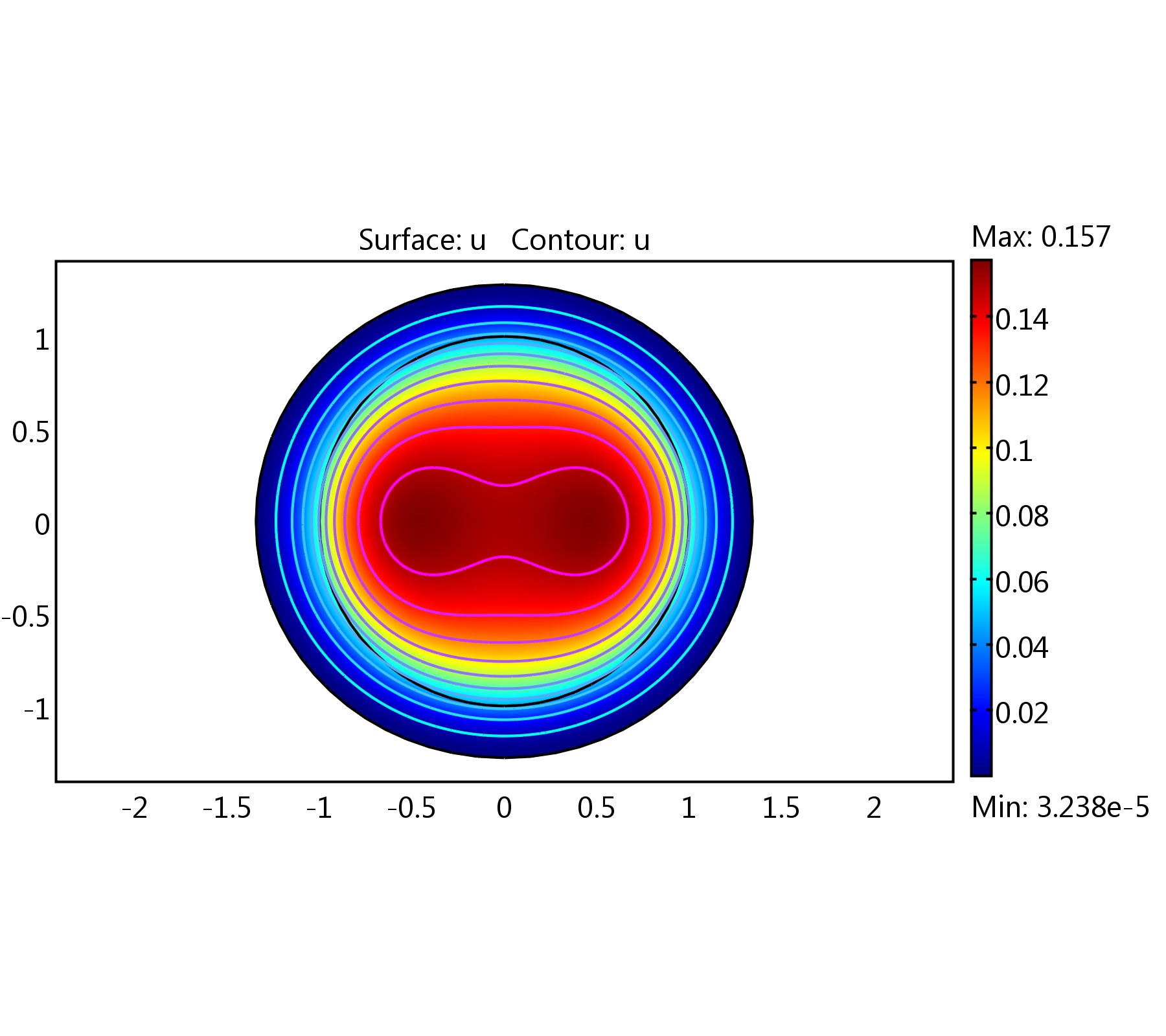
Figure 1. The solution of Problem (P) by employing the first method and considering $\mu=(1+2x^{2}+y^{2})\chi_{B}$ after three iterations.

Figure 2. The quantity $|\nabla u|$ on the boundary of the solution in Figure 1.

Figure 3. The colored part shows the solution $\Omega_{1}$, after first iteration, where support of $\mu$ is the polygon and the initial guess ($\Omega_{0}$) is a ball.

Figure 4. Final domain after four iterations when $\mu=1.5\chi_{P}$ and where $P$ is the polygon.

Figure 5. The value of $|\nabla u|$ on the boundary of the solution after four iterations.

Figure 6. The first iteration for $\mu=11\chi_{P},\,$ where $P$ is the polygon. Initial guess is a ball with center at origin.

Figure 7. Final quadrature domain when $\mu=11\chi_{P}$ and where $P$ is the polygon.

Figure 8. The surface of the solution $u$ and a cross section line.

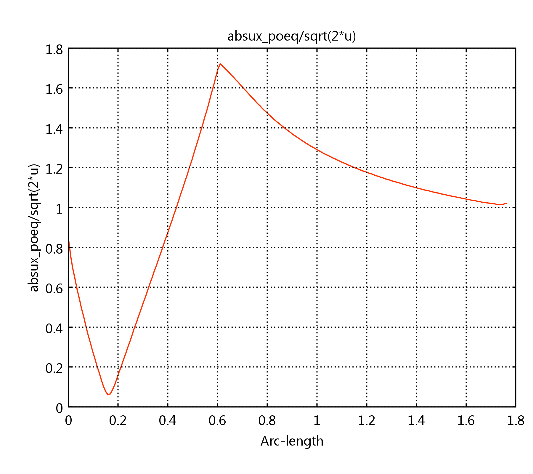
Figure 9. The amount of $\frac{|\nabla u|}{\sqrt{2u}}$ on the cross section line in figure (8).

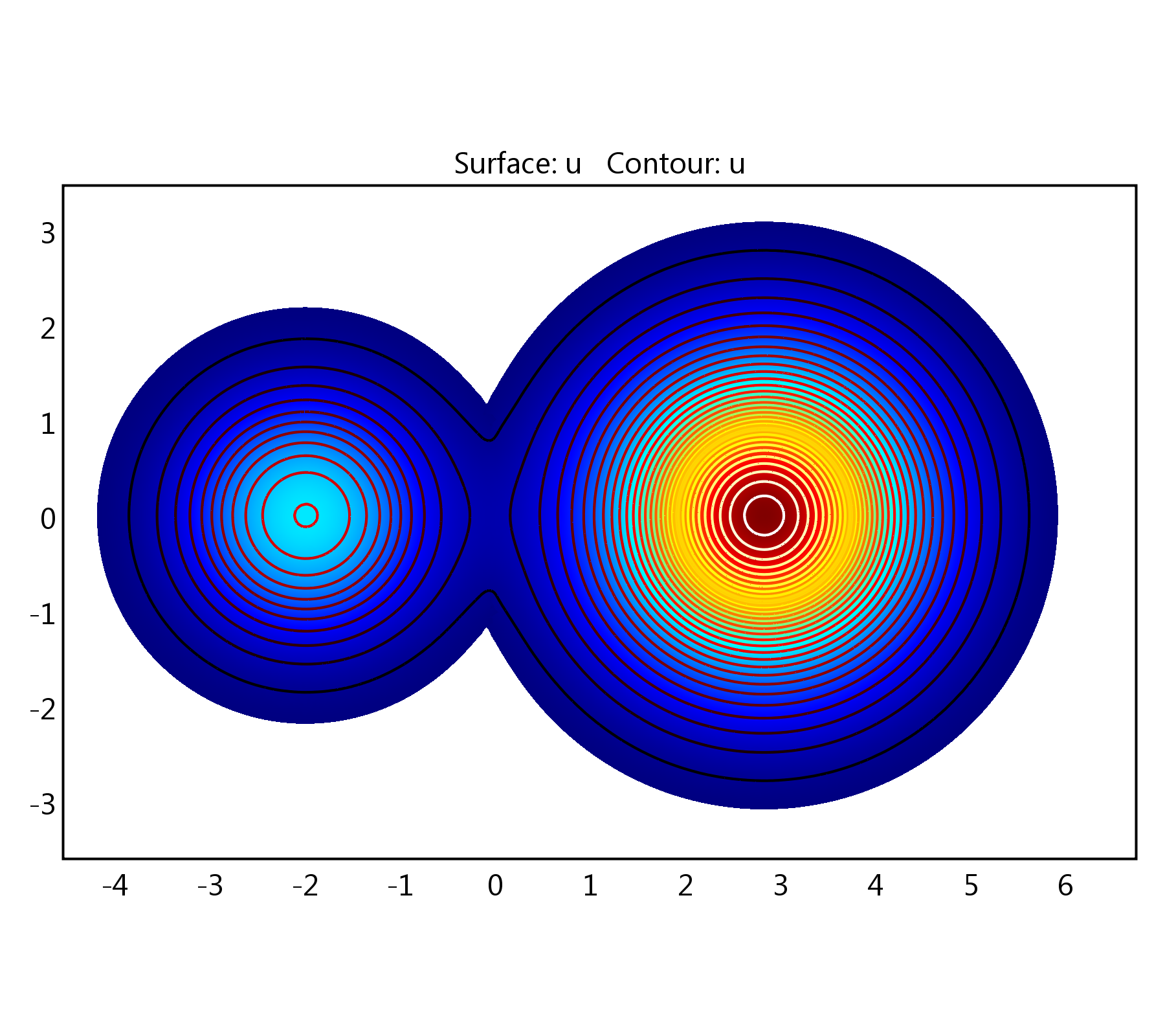
Figure 10. The quadrature domain corresponding to the solution of (6.1) for $t=5$.

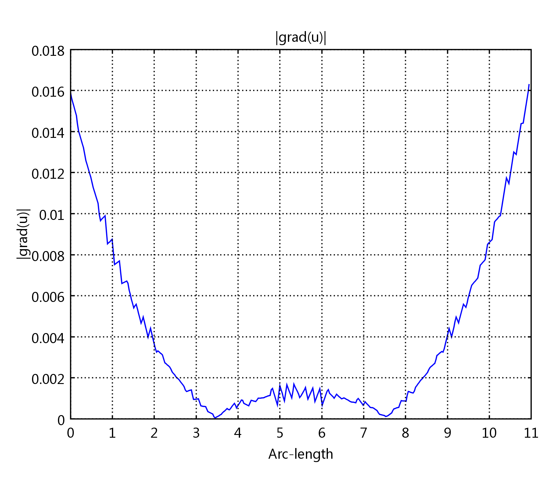
Figure 11. The quantity of $|\nabla u|$ on the boundary of the solution of (6.1) for $t=5$.

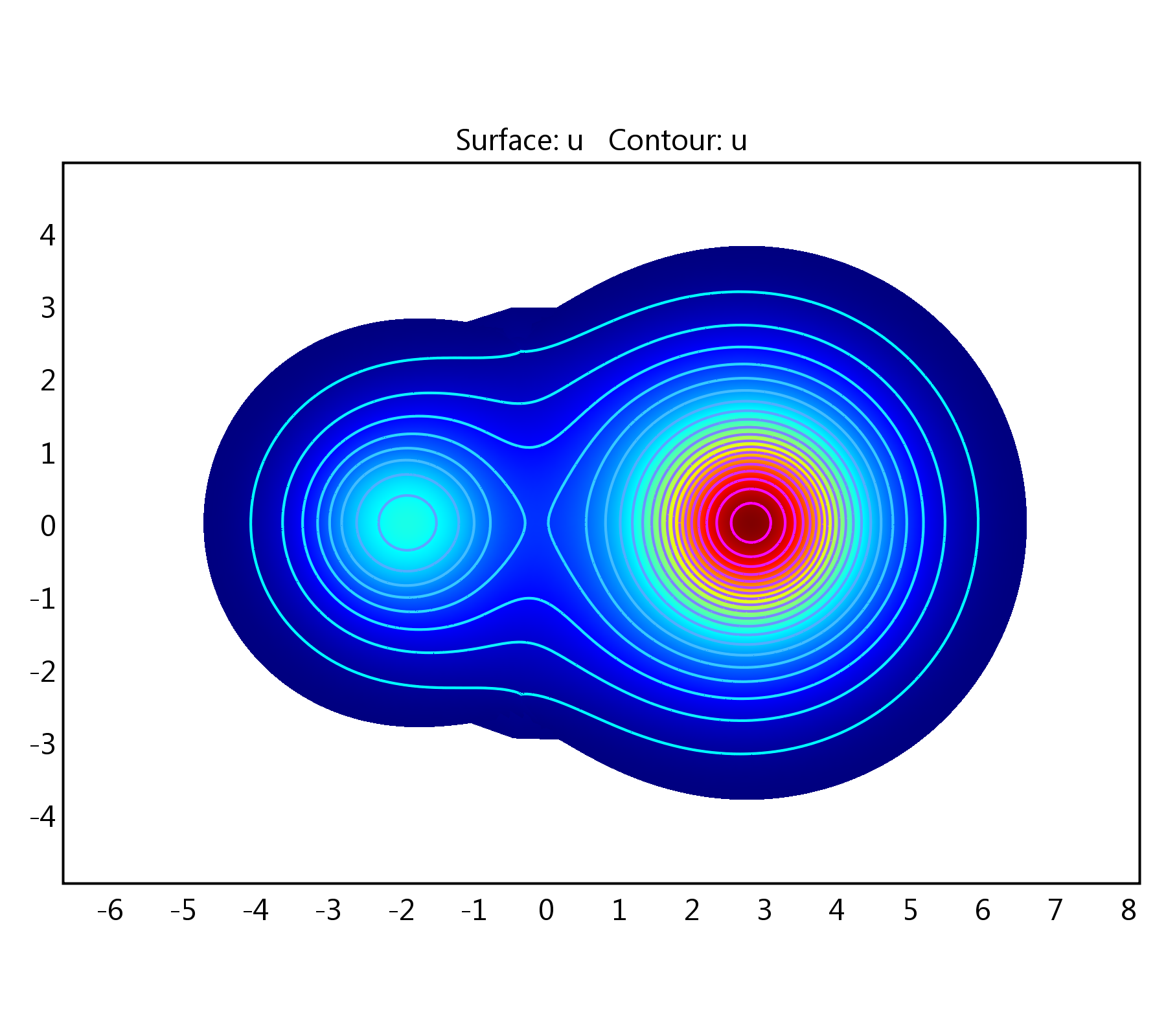
Figure 12. The quadrature domain corresponding to the solution of (6.1) for $t=6$.

Acknowledgments: This problem was suggested by Professor Henrik Shahgholian. We wish to thank him for plentiful discussions and profitable suggestions.