Speed limits for quantum gates in multi-qubit systems

Abstract

We use analytical and numerical calculations to obtain speed limits for various unitary quantum operations in multi-qubit systems under typical experimental conditions. The operations that we consider include single-, two- and three-qubit gates, as well as quantum state transfer in a chain of qubits. We find in particular that simple methods for implementing two-qubit gates generally provide the fastest possible implementations of these gates. We also find that the three-qubit Toffoli gate time varies greatly depending on the type of interactions and the system’s geometry, taking only slightly longer than a two-qubit controlled-NOT (CNOT) gate for a triangle geometry. The speed limit for quantum state transfer across a qubit chain is set by the maximum spin wave speed in the chain.

I Introduction

There are a number of candidate physical systems for the implementation of qubits in a future quantum computer QubitReviews . Single-, two- and three-qubit gates have been implemented in some of these systems in the past few years. Various other quantum-information-related tasks based on collective manipulation of qubits have also been demonstrated on larger systems QubitReviews .

As qubit systems advance towards large-scale demonstrations and practical applications, it becomes increasingly important to optimize the time required to implement the different operations, such that the maximum number of operations is achieved within the coherence time of the system. This goal is the main motivation of this work.

The question of time-optimal control has already been discussed in a number of studies in the literature. For example, Refs. Barenco ; Yuan considered optimized constructions of general quantum gates using sequences of basic gates. References MandelstamTamm discussed the relationship between speed limits on quantum gates and the different energy scales in a physical system, while Refs. GeometricArguments explored the analogy between the problem of finding the minimum times for quantum gates and the problem of finding geodesics in curved spaces. These ideas were applied in Ref. Vidal in order to find a general recipe for calculating speed limits for two-qubit gates. The time-optimal implementation of the quantum Fourier transform in multi-qubit systems was analyzed in Ref. SchulteHerbrueggen , and the time-optimal implementation of the CNOT gate on indirectly coupled qubits was studied in Ref. Carlini . References Spoerl ; Stojanovic performed numerical calculations in order to determine the minimum time required for quantum gates in specific experimental setups based on superconducting qubits. The speed limit on quantum state transfer in long spin chains has also been studied recently Osborne ; Caneva .

Here we consider a number of important operations in a variety of possible setups, with varying degrees of single-qubit control and inter-qubit coupling mechanisms. We use analytical arguments and numerical calculations based on optimal control theory in order to give speed limits for these operations.

The paper is organized as follows: In Sec. II we introduce the different possible setups, with varying forms of single-qubit controls and interactions. We then discuss the speed limits of single-qubit gates (Sec. III), two-qubit gates (Sec. IV) and three-qubit gates (Sec. V). In Sec. VI we discuss the problem of quantum state transfer. We conclude with a brief summary of the results in Sec. VII.

II Different types of qubits and their coupling

Over the years, various physical systems and designs have been proposed and demonstrated as implementations of qubits. This variety means that the degree of control in qubit manipulation and the physical mechanisms for coupling between qubits vary from one system to another. In some cases, the qubit is formed by the lowest two energy levels of a multi-level quantum system, adding complications to the control requirements of the qubit. Here we shall focus on “good” qubits, where a description with only two quantum states provides a good approximation of the physical system.

With the assumption of two-state qubits, the single-qubit Hamiltonian can be expressed in terms of the two-dimensional Pauli matrices $\hat{\sigma}_{\alpha}$ (with $\alpha=x$, $y$ or $z$):

$$\hat{H}=-\frac{\Delta(t)}{2}\hat{\sigma}_{x}-\frac{\epsilon(t)}{2}\hat{\sigma}_{z},$$ (1)

where the time dependence in Eq. (1) suggests that both $\Delta$ and $\epsilon$ are tunable. Some experimental setups (e.g. early experiments on superconducting qubits) have only one tunable parameter, typically expressed as $\epsilon$ in Eq. (1). We shall consider both cases below.

Driving signals used for the manipulation of the qubits can be applied through the tunable parameters in the Hamiltonian. We shall assume that any arbitrary driving signal can be applied to the system. In other words, we look for the fastest implementation of quantum operations in the space of all possible control signals.

The coupling Hamiltonian between two qubits is typically of Ising or Heisenberg form. The former is described by the Hamiltonian

$$\hat{H}_{\rm I}=J\hat{\sigma}_{z}^{(i)}\otimes\hat{\sigma}_{z}^{(j)},$$ (2)

while the latter is described by the Hamiltonian

$$\hat{H}_{\rm H}=J\left(\hat{\sigma}_{x}^{(i)}\otimes\hat{\sigma}_{x}^{(j)}+\hat{\sigma}_{y}^{(i)}\otimes\hat{\sigma}_{y}^{(j)}+\hat{\sigma}_{z}^{(i)}\otimes\hat{\sigma}_{z}^{(j)}\right).$$ (3)

where $J$ is the coupling strength and the superscripts $i$ and $j$ denote the two coupled qubits. There are situations where the coupling strength is tunable, e.g. using additional coupler elements in the system. However, since we are interested in the speed limits for performing multi-qubit gates, we shall assume that one would want to set $J$ at its maximum achievable value and therefore treat $J$ as a fixed parameter in the calculations below. It is worth mentioning here that it is possible in principle to have fixed values of $\Delta$ and $\epsilon$ and still be able to obtain the desired gates via the modulation of $J$, an approach sometimes referred to as parametric coupling Bertet .

The parameters of the single-qubit Hamiltonian are typically much larger than the inter-qubit coupling strength, i.e. $J\ll\Delta,\epsilon$. This separation in energy scales simplifies the process of identifying the central elements in the speed limits found in our calculations, and it makes the results easily applicable to different setups.

III Single-qubit gates

Since the parameters of the single-qubit Hamiltonian are typically much larger than the inter-qubit coupling strength, one can ignore inter-qubit interactions when performing single-qubit gates. Furthermore, performing single-qubit gates typically requires a negligibly short duration compared to the duration required for performing a two- or multi-qubit gate, such that the time required for performing single-qubit gates is usually ignored for purposes of evaluating the computational cost of a given multi-qubit task.

Ignoring interactions, and thus reducing the problem of finding optimal pulses and speed limits for performing a given single-qubit gate to a single-qubit problem, the task at hand becomes straightforward. A common situation is that in which one of the two parameters, say $\epsilon$, is tunable over a much larger range than the other one, while the other parameter is either fixed or tunable over a much smaller range. A rotation by an angle $\beta$ about an axis that makes an angle $\theta$ with the $z$ axis and an angle $\phi$ with the $xz$ plane can be implemented as follows: rotate the state by an angle $-\phi$ about the $z$ axis, set the Hamiltonian to $\Delta(\hat{\sigma}_{x}+\hat{\sigma}_{z}\cot\theta)/2$ and let it act for a duration $\beta\sin\theta/\Delta$, and finally rotate the state by an angle $\phi$ about the $z$ axis. The first and last steps are fast operations that are implemented by setting $\epsilon$ to a value that is much larger than $\Delta$. As a result, the duration of the second step is the limiting factor for the minimum time required for implementing the desired rotation. One can therefore say that the speed limit is set by the smaller of the two qubit parameters (or more accurately the smaller of the largest achievable values of the two parameters), which in the above example is $\Delta$.

IV Two-qubit gates

We start the discussion of finding the speed limits for two-qubit gates by mentioning two approaches that might seem promising at first sight, but to our knowledge are not always applicable to the problem at hand. First, there are expressions for the speed limits of quantum operations based on the energy and the spread in energy of the quantum state MandelstamTamm . The reason why these arguments do not apply straightforwardly here can be seen by considering two qubits with a coupling strength that is much smaller than the inter-qubit detuning. The energy scales of the combined system are then, to a very good approximation, set by the individual qubit energies and their detuning from each other. The coupling strength only slightly modifies the energy eigenstates and eigenvalues. The coupling strength must, however, be the limiting factor for performing two-qubit gates. The larger energy scales can be used to set a lower bound on the required gate time (i.e. an upper bound on the speed). However, the coupling strength would give a much higher lower bound.

The other approach is that in which two-qubit gates are visualized using geometric representations, and the process of performing a two-qubit gate is seen as the motion of the system’s propagator through the space of all two-qubit quantum operations GeometricArguments . This approach does indeed provide an intuitive view of the problem and can be very useful in calculations. Furthermore, for the case of fully tunable single-qubit parameters, i.e. the case where one can assume to have (i) a fixed interaction Hamiltonian with no single-qubit terms and (ii) the ability to perform fast single-qubit gates, Ref. Vidal gives a recipe for determining the speed limit of any two-qubit gate with any interaction Hamiltonian. However, it is not obvious that the speed limits provided by this approach apply to the case of fixed $\Delta$, which is relevant to a good number of realistic experiments.

Four representative gates that are commonly studied in the literature are: iSWAP, controlled-Z (CZ), CNOT and $\sqrt{\rm SWAP}$. There are a number of simple methods that can be obtained using intuition for the implementation of these gates assuming a given (fixed) coupling strength $J$ and tunable single-qubit parameters. The basic techniques, which can also be shown to be time-optimal Vidal , are summarized in the following Schuch :

iSWAP Gate: The standard approach to implementing the iSWAP gate with Ising interactions is to put the two qubits in resonance with each other, i.e. setting $\Delta_{1}=\Delta_{2}=\Delta$, with $\epsilon_{1}=\epsilon_{2}=0$ and $J\ll\Delta$:

$$\hat{H} = -\frac{\Delta_{1}}{2}\hat{\sigma}_{x}^{(1)}-\frac{\Delta_{2}}{2}\hat{\sigma}_{x}^{(2)}+J\hat{\sigma}_{z}^{(1)}\otimes\hat{\sigma}_{z}^{(2)}$$

$$\approx -\frac{\Delta_{1}}{2}\hat{\sigma}_{x}^{(1)}-\frac{\Delta_{2}}{2}\hat{\sigma}_{x}^{(2)}+J\left(\hat{\sigma}_{+}^{(1)}\otimes\hat{\sigma}_{-}^{(2)}+\hat{\sigma}_{-}^{(1)}\otimes\hat{\sigma}_{+}^{(2)}\right)$$

where the operators $\hat{\sigma}_{\pm}$ are raising and lowering operators that excite or de-excite the individual qubits between their single-qubit energy eigenstates, which in this case are the eigenstates of $\hat{\sigma}_{x}$. When allowed to act for a duration $t=\pi/(2J)$, the Hamiltonian in Eq. (LABEL:Eq:iSWAPHamiltonian) effects an iSWAP gate, in addition to two single-qubit rotations.

Controlled-$\pi$-phase gate: With Ising interactions, the controlled-$\pi$-phase (or CZ) gate can be performed by setting $\Delta_{1}=\Delta_{2}=0$:

$$\hat{H}=-\frac{\epsilon_{1}}{2}\hat{\sigma}_{z}^{(1)}-\frac{\epsilon_{2}}{2}\hat{\sigma}_{z}^{(2)}+J\hat{\sigma}_{z}^{(1)}\otimes\hat{\sigma}_{z}^{(2)},$$ (5)

with no conditions on $\epsilon_{1}$ and $\epsilon_{2}$. When allowed to act for a duration $t=\pi/(4J)$, the Hamiltonian in Eq. (5) effects a CZ gate, in addition to two single-qubit rotations and an (unimportant) overall phase factor.

CNOT gate: The CNOT gate can be obtained by combining the CZ gate with two single-qubit gates. These are $\pi/2$ pulses applied to the target qubit before and after the CZ gate. As a result, the amount of time required to obtain the CNOT gate using this approach is approximately equal to the amount of time required for the CZ gate, i.e. $\pi/(4J)$ with Ising interactions.

$\sqrt{\rm\bf SWAP}$ gate: The $\sqrt{\rm SWAP}$ gate is more naturally obtained with Heisenberg interactions. In this case, one sets $\Delta_{1}=\Delta_{2}$ and $\epsilon_{1}=\epsilon_{2}$, and after a time $t=\pi/(8J)$ one obtains the $\sqrt{\rm SWAP}$ gate.

Numerical calculations: Here we use numerical calculations to find the speed limits for a number of standard two-qubit gates. The method is based on optimal control theory for finding driving pulses that maximize the gate fidelity Khaneja . The fidelity is essentially a measure of the overlap between the numerically calculated gate and the desired target gate. Here we use the definition

$${\rm Fidelity}=\left|\frac{{\rm Tr}\left\{U_{\rm Target}^{\dagger}U_{\rm Numerical}\right\}}{2^{n}}\right|^{2},$$ (6)

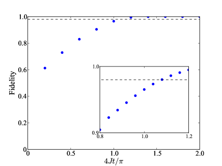
Figure 1: (Color online) The fidelity of the CNOT gate for the pulse obtained using optimal control theory as a function of the allowed time $t$ (plotted in the combination $4Jt/\pi$) in the case of Ising interactions and fixed values of $\Delta$. The parameters are $\Delta_{2}/\Delta_{1}=0.9$ and $J/\Delta_{1}=0.01$. The dashed line represents a possible threshold fidelity for identifying the minimum gate time. Here this threshold is set at 0.98.

where $U_{\rm Target}$ and $U_{\rm Numerical}$ are, respectively, the target gate and any given unitary operation (which is obtained from solving the Schrödinger equation with a given driving signal), and $n$ is the number of qubits (here $n=2$). When the gate time (which is a variable parameter in the calculations) is set to a small value, the maximum achievable fidelity is substantially smaller than unity. As the allowed time is increased, the maximum achievable fidelity increases, until at a certain value of the allowed time the fidelity reaches the value one and remains at that value for larger times SchulteHerbrueggen ; Caneva . In other words, when plotted as a function of the allowed time, the fidelity exhibits non-analytic behaviour as it suddenly hits the value one and remains there. The time at which the fidelity reaches unity defines the minimum gate time, which can alternatively be expressed as the speed limit. A commonly used procedure for deducing speed limits is to set a threshold value for the fidelity (say 99%) and numerically identify the minimum time required in order to attain this fidelity. This procedure is illustrated in Fig. 1.

Here we use an alternative procedure that avoids one of the drawbacks of the above procedure, namely the slow convergence of the pulse-optimization algorithm when the fidelity approaches its asymptotic value (when plotted as a function of iteration number). We calculate the maximum achievable fidelity for times varying between zero and an estimated value for the minimum gate time. The results of such a calculation are plotted in Fig. 2 for the case of the $\sqrt{\rm SWAP}$ gate with Heisenberg interactions. We can see that the results fit very well with a function that gives the gate time $\pi/(8J)$. The sine function used in the figure was used as a ‘trial’ fitting function; it was inspired by the behaviour of single-qubit gates but turned out to produce an excellent fit in this case as well. We note here that this alternative method (i.e. the method where one looks away from the threshold region in order to identify the minimum gate time) has not been used in the literature in the context of optimal-control theory. More complicated fitting functions might be required when applying this method to systems with more than two qubits. However, it would be interesting to explore in the future the usefulness of this approach to similar problems. We shall use this method when identifying the minimum gate time in the calculations below.

It is worth mentioning that the numerical method used here is guaranteed to give the optimal pulses, and therefore the correct speed limit, if given sufficient computation time Brif . Small-scale calculations could produce results that overestimate the speed limit, because the algorithm might not converge to the optimal pulses with the given calculation parameters. The availability of known speed limits in the literature (e.g. in Ref. Vidal ) for some physical setups and gates allows us to characterize the performance of our calculations with a given set of parameters. We find that in most cases we obtain the correct speed limits to within a few percent with relatively small-scale calculations.

The results for the deduced gate times are summarized in Table 1. The numerical calculations are performed with 500 time steps and $10^{4}$ iterations. With these parameters a single data point takes a calculation time on the order of one hour. We run each calculation a few times with a variety of initial pulses in order to minimize the chances of slow convergence towards the optimal pulse, which is a possibility given the fact that we do not know the structure of the fidelity landscape. For fixed-$\Delta$ calculations, we set $\Delta_{2}/\Delta_{1}=0.9$ and $J/\Delta_{1}=0.01$. The speed limits for the case of tunable $\Delta_{i}$ are known, and using them we can see that our relatively small-scale calculations produce a very good approximation to the speed limit in most cases. This observation gives us confidence in the convergence behaviour of the calculations.

The main observation that we make from the results in Table 1 is that all the results remained unchanged whether the parameters $\Delta_{i}$ were taken to be fixed or tunable, a result that is not a prioi obvious. In some cases, the calculations with tunable $\Delta$ produced higher estimates for the minimum gate time than the calculations with fixed $\Delta$, even though the tunable-$\Delta$ case has more tunable parameters and must therefore result in gates that are at least as fast as those obtained in the fixed-$\Delta$ case. It seems, however, that the presence of additional tunable parameters can have the effect of slowing down the convergence of the optimization algorithm, which we see for some of the cases considered in Table 1. On the other hand, one case where the fixed-$\Delta$ result is substantially higher than the tunable-$\Delta$ result is that of the iSWAP gate with Ising interactions. The speed limit that we find numerically for the fixed-$\Delta$ case is about 25% higher than that for the tunable $\Delta$ case. However, this difference is again caused by numerical inaccuracies. In the case where $J\ll|\Delta_{1}-\Delta_{2}|\ll\Delta_{1}$ it is known that one can approach a gate time of $\pi/(2J)$, and this fast gate is achieved by strongly driving the two qubits such that they are effectively tuned into resonance with each other Ashhab . Since the fixed-$\Delta$ speed limit cannot be higher than the tunable-$\Delta$ speed limit, one can conclude that the speed limit is $\pi/(2J)$ in both cases. The fact that a large-amplitude, high-frequency driving pulse is needed in order to achieve the speed limit (assuming that this is the only way to achieve the speed limit) might partly explain why the algorithm is not converging to the optimal pulses. Another partial explanation of the relatively large gate time obtained in this case could be the fact that $J/\Delta_{1}=0.01$, which could increase the minimum gate time by a few percent.

It is also worth noting here that even though the Heisenberg interaction Hamiltonian has more terms than the Ising interaction Hamiltonian, which generally results in larger frequency shifts and gaps in spectroscopy measurements, it is not the case that Heisenberg interactions will always result in faster two-qubit gates. One case that might be particularly surprising at first sight is that of the iSWAP gate. The term proportional to $(\hat{\sigma}_{+}^{(1)}\otimes\hat{\sigma}_{-}^{(2)}+\hat{\sigma}_{-}^{(1)}\otimes\hat{\sigma}_{+}^{(2)})$ is larger in the case of Heisenberg interactions. However, the presence of the $\hat{\sigma}_{z}^{(1)}\otimes\hat{\sigma}_{z}^{(2)}$ term in some sense has the effect of slowing down the iSWAP-gate dynamics, such that Heisenberg interactions and Ising interactions give the same minimum gate times.

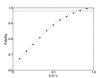
Figure 2: (Color online) The fidelity of the $\sqrt{\rm SWAP}$ gate for the pulse obtained using optimal control theory as a function of the allowed time $t$ (plotted in the combination $8Jt/\pi$) in the case of Heisenberg interactions and fixed values of $\Delta$. The parameters are $\Delta_{2}/\Delta_{1}=0.9$ and $J/\Delta_{1}=0.01$. The dashed line represents, as an example, a threshold fidelity of 0.98. The red dotted line is the function $(5/8)+(3/8)\times\sin(4Jt)$. Note that the value $5/8$ is the fidelity of the unit matrix with the $\sqrt{\rm SWAP}$ gate.

Table 1: Minimum times required for various two-qubit gates and physical realizations. The analytical expressions given below are extracted from the numerical calculations: for each calculation we identify the value of the time that gives a good fit to a figure similar to Fig. 2 (the sine function used for the fidelity dependence always provided a good fit to the data). In the fixed-$\Delta$ calculations, we set $\Delta_{2}/\Delta_{1}=0.9$ and $J/\Delta_{1}=0.01$.

Gate		CNOT		CZ		iSWAP		$\sqrt{\rm SWAP}$
Matrix		$\left(\begin{array}[]{cccc}1&0&0&0\\ 0&1&0&0\\ 0&0&0&1\\ 0&0&1&0\end{array}\right)$		$\left(\begin{array}[]{cccc}1&0&0&0\\ 0&1&0&0\\ 0&0&1&0\\ 0&0&0&-1\end{array}\right)$		$\left(\begin{array}[]{cccc}1&0&0&0\\ 0&0&i&0\\ 0&i&0&0\\ 0&0&0&1\end{array}\right)$		$\left(\begin{array}[]{cccc}1&0&0&0\\ 0&\frac{1+i}{2}&\frac{1-i}{2}&0\\ 0&\frac{1-i}{2}&\frac{1+i}{2}&0\\ 0&0&0&1\end{array}\right)$
Ising, fixed $\Delta$		$\displaystyle\frac{\pi}{4J}\times$ 1.12		$\displaystyle\frac{\pi}{4J}\times$ 1.14		$\displaystyle\frac{\pi}{2J}\times$ 1.25		$\displaystyle\frac{3\pi}{8J}\times$ 1.00
Ising, tunable $\Delta$		$\displaystyle\frac{\pi}{4J}\times$ 1.17		$\displaystyle\frac{\pi}{4J}\times$ 1.26		$\displaystyle\frac{\pi}{2J}\times$ 1.04		$\displaystyle\frac{3\pi}{8J}\times$ 1.03
Heisenberg, fixed $\Delta$		$\displaystyle\frac{\pi}{4J}\times$ 1.01		$\displaystyle\frac{\pi}{4J}\times$ 1.00		$\displaystyle\frac{\pi}{2J}\times$ 1.04		$\displaystyle\frac{\pi}{8J}\times$ 1.01
Heisenberg, tunable $\Delta$		$\displaystyle\frac{\pi}{4J}\times$ 1.10		$\displaystyle\frac{\pi}{4J}\times$ 1.00		$\displaystyle\frac{\pi}{2J}\times$ 1.02		$\displaystyle\frac{\pi}{8J}\times$ 1.00

V Three-qubit gates

The most well-known three-qubit gate is the Toffoli gate. This gate is also known as the controlled-controlled-NOT gate, because it applies the NOT operation to the target qubit when both control qubits are in the state $\left|1\right\rangle$. It has been known for some time that the Toffoli gate can be constructed from six CNOT gates, in addition to a number of single-qubit gates. Recently it has been shown that this number (i.e. six) is the minimum number of CNOT gates required in order to construct the Toffoli gate Shende . Different constructions based on general conditional gates have also been proposed, reducing the Toffoli-gate time from 6 to 3.5 times that CNOT gate time Barenco . An optimal-control-theory-related calculation based on certain forms of pulses has found a gate time of about 2.2 times the CNOT gate time for qubits coupled in a triangle geometry Yuan .

We have performed numerical calculations in order to determine the minimum time required in order to obtain the Toffoli gate for a Hamiltonian with pairwise interaction terms given by Eq. (2) or Eq. (3). We should stress here that these calculations are independent of the results mentioned above. The reason is that the gate-counting calculations assume that the different gates are applied as separate, well-defined units, and in some calculations it is assumed that the two-qubit gates used in the construction are taken from a specific class of gates (e.g. conditional gates). One can therefore expect that it should be possible to obtain a shorter minimum time for the Toffoli gate by considering essentially all the possible driving pulses.

The results are summarized in Table 2. There we show results where all coupling strengths are equal (allowing small differences between the different coupling strengths does not change the main results). We only present results for fixed-$\Delta$ calculations, because the variable-$\Delta$ calculations did not produce any useful results within any reasonable calculation time. In addition to the fact that our procedure typically overestimates the minimum gate time, we would like to point out that the results of the calculations also showed stronger dependence on the guess pulses than in the case of two-qubit gates (the data also did not result in smooth fitting functions as shown in Fig. 2). We therefore cannot exclude the possibility that some of the expressions in Table 2 are substantially larger than the true minimum gate time. However, for the triangle geometry, we find Toffoli gate times that are smaller than twice the minimum time required for a CNOT gate with the same coupling strength. In this case, we can have a good level of confidence that the results are at least close to the true minimum gate time, since it seems implausible that the Toffoli gate could be faster than the CNOT gate for the same value of the coupling strengths. From the results shown in the table, we can also conclude that having the qubits connected in a triangle geometry would be desirable for purposes of implementing fast three-qubit gates. We should point out here that the results presented here give faster gates than any results for the maximum speed of Toffoli gates in the literature Barenco ; Yuan . In particular, one can compare the factor 1.9 in Table 2 with the corresponding factor of 2.2 in Ref. Yuan : an improvement of about 15%.

Table 2: Minimum times required for the three-qubit Toffoli gate with various physical realizations. The results are given in terms of the CNOT gate time, i.e. $\pi/(4J)$. The numerical calculations are performed with $\sim 10^{4}$ time steps and $\sim 10^{4}$ iterations (a single data point now takes a calculation time on the order of one day). The parameters $\Delta_{i}$ are fixed in the calculations, and we set $\Delta_{2}/\Delta_{1}=0.9$, $\Delta_{3}/\Delta_{1}=0.82$ and $J/\Delta_{1}=0.01$ for all of the coupling terms.

Geometry		chain		chain		triangle
Target qubit		center qubit		side qubit		any qubit
Ising		3.8		3.8		1.9
Heisenberg		2.8		2.6		1.4

VI Quantum state transfer in a chain of qubits

Another operation in multi-qubit systems that has received considerable attention in recent years is that of quantum state transfer across a chain of qubits SpinChainPapers . In this section we provide analytical expressions for the speed limit of state transfer across a long chain.

The Hamiltonian for a qubit chain with nearest neighbour interactions is given by

$$\hat{H}=\sum_{i=1}^{N}\left(-\frac{\Delta_{i}}{2}\hat{\sigma}_{x}^{(i)}-\frac{\epsilon_{i}}{2}\hat{\sigma}_{z}^{(i)}\right)+\sum_{i=1}^{N-1}J_{i}\hat{\sigma}_{z}^{(i)}\otimes\hat{\sigma}_{z}^{(i+1)}$$ (7)

for the case of Ising interactions and

$$\hat{H} = \sum_{i=1}^{N}\left(-\frac{\Delta_{i}}{2}\hat{\sigma}_{x}^{(i)}-\frac{\epsilon_{i}}{2}\hat{\sigma}_{z}^{(i)}\right)+\sum_{i=1}^{N-1}J_{i}\times$$ (8)

$$\left(\hat{\sigma}_{x}^{(i)}\otimes\hat{\sigma}_{x}^{(i+1)}+\hat{\sigma}_{y}^{(i)}\otimes\hat{\sigma}_{y}^{(i+1)}+\hat{\sigma}_{z}^{(i)}\otimes\hat{\sigma}_{z}^{(i+1)}\right).$$

for Heisenberg interactions. The case with fixed and generally disordered values of $\Delta_{i}$ and/or $J_{i}$ leads to serious complications (such as Anderson localization), and we therefore do not consider this case. For the case of fixed, uniform values of $\Delta_{i}$ and $J_{i}$ or the case of tunable $\Delta_{i}$ and uniform $J_{i}$, we can use arguments from band theory to find the speed limit for state transfer.

The state-transfer process can be thought of as the process of wave propagation through the chain, as discussed in Ref. Osborne . The speed limit is then determined by the maximum group velocity of a wave packet traveling through the chain. We also observe here that wave propagation cannot be sped up through the application of nonuniform external fields. We can therefore calculate the maximum wave speed assuming a uniform external field (i.e. time- and position-independent values of $\Delta_{i}$ and $\epsilon_{i}$). For the case of Ising interactions, we start by noting that if we take $\Delta=0$, then the operator $\hat{\sigma}_{z}^{(i)}$ commutes with the Hamiltonian, prohibiting “propagation”. We therefore conclude that the condition $\Delta\gg J$ is optimal for maximizing the propagation speed. With this assumption, the wave function that describes a wave with momentum $k$ (with $-\pi<k<\pi$) is given by

$$\left|k\right\rangle=\sum_{j=1}^{N}e^{ikj}\hat{\sigma}_{z}^{(j)}\left|\sigma_{x}^{(1)}=1,\cdots,\sigma_{x}^{(N)}=1\right\rangle.$$ (9)

The energy spectrum of these waves is given by $E_{k}=2J\cos k$. The group velocity of the wave is given by

$$v_{k}=\frac{dE}{dk}=-2J\sin k,$$ (10)

which has a maximum at $k=\pi/2$, and the maximum is given by $2J$. The minimum time for the wave to traverse a chain of length $N$ is attained when the wave is initialized and set to travel at this maximum wave speed. Ignoring chain-length-independent contributions at the beginning and end of the transfer process, the minimum transfer time is therefore given by

$$T_{\rm min}=\frac{N}{2J}.$$ (11)

It is worth noting that $T_{\rm min}$ is faster by a factor of $\pi$ than the sequential application of iSWAP operations across the chain. We also note that the expression for the maximum wave speed given above can be found in the literature, e.g. in Ref. Happola .

For the case of Heisenberg interactions, the speed of wave propagation is independent of the external fields. Taking $\Delta\gg J$, $\epsilon=0$, and assuming only one excitation in the system, the problem reduces to that with Ising interactions but with twice the coupling strength: the $\hat{\sigma}_{x}^{(i)}\otimes\hat{\sigma}_{x}^{(j)}$ term has no effect on the dynamics, and

$$\hat{\sigma}_{y}^{(i)}\otimes\hat{\sigma}_{y}^{(j)}+\hat{\sigma}_{z}^{(i)}\otimes\hat{\sigma}_{z}^{(j)}=2\left(\hat{\sigma}_{+}^{(i)}\otimes\hat{\sigma}_{-}^{(j)}+\hat{\sigma}_{-}^{(i)}\otimes\hat{\sigma}_{+}^{(j)}\right).$$ (12)

The minimum transfer time is therefore given by

$$T_{\rm min}=\frac{N}{4J}.$$ (13)

This expression is essentially the same as the one given in Ref. Osborne . Using numerical calculations Ref. Caneva found a time that is a few percent higher (note that there is a factor-of-two difference between Eq. (8) and the Hamiltonian used in Ref. Caneva ).

Even though the maximum wave speed sets an upper limit to the speed of quantum-state transfer, one still needs to make sure that the quantum state is transferred without distortion. The authors of Ref. Osborne assumed that one has access to a limited number of qubits in the chain and analyzed the dispersion of the propagating wave. They found that if one has access to a number that is at least on the order of $\sqrt{N}$ at both ends of the chain, then state transfer can occur with high fidelity. The authors of Ref. Caneva assumed access to all of the qubits and, using numerical calculations, demonstrated that by using a ‘carrier’ external field (e.g. a harmonic-oscillator potential that moves along the chain and carries the quantum state as it moves along) the dispersion of the wave can also be prevented, and high-fidelity state transfer is possible.

VII Conclusion

We have derived a number of speed limits, or lower bounds on the required time, for various quantum operations in various setups that correspond to a variety of experimental conditions. Single-qubit operation speeds are limited by the smaller of the Pauli-matrix coefficients in the Hamiltonian. We have used optimal control theory to obtain speed limits for a few well-known two-qubit gates and the three-qubit Toffoli gate. As expected, two-qubit gate speeds are limited by the inter-qubit coupling strength. The Toffoli gate requires approximately three times the minimum time required for a CNOT gate in a chain geometry and less than twice the minimum time required for a CNOT gate in a triangle geometry. Finally, we have used arguments from condensed-matter physics to derive the speed limit for quantum state transfer in a qubit chain. The expressions that we find agree with analytical results known in the literature and also with recent numerical results.

References

- (1) I. Buluta, S. Ashhab, and F. Nori, Rep. Prog. Phys. 74, 104401 (2011); T. D. Ladd, F. Jelezko, R. Laflamme, Y. Nakamura, C. Monroe, J. L. O’Brien, Nature 464, 45 (2010).
- (2) A. Barenco, C. H. Bennett, R. Cleve, D. P. DiVincenzo, N. Margolus, P. Shor, T. Sleator, J. A. Smolin, and H. Weinfurter Phys. Rev. A 52, 3457 (1995).
- (3) H. Yuan and N. Khaneja, Phys. Rev. A 84, 062301 (2011).
- (4) L. Mandelstam and I. G. Tamm, J. Phys. USSR 9, 249 (1945); N. Margolus and L. B. Levitin, Physica D 120, 188 (1998); P. Pfeifer, Phys. Rev. Lett. 70, 3365 (1993); V. Giovannetti, S. Lloyd, and L. Maccone, Phys. Rev. A 67, 052109 (2003).
- (5) N. Khaneja, R. Brockett, and S. J. Glaser, Phys. Rev. A 63, 032308 (2001); Y. Makhlin, Quant. Info. Proc. 1, 243 (2002); J. Zhang, J. Vala, S. Sastry, and K. B. Whaley, Phys. Rev. A 67, 042313 (2003); N. Khaneja, B. Heitmann, A. Spörl, H. Yuan, T. Schulte-Herbrüggen, and S. J. Glaser, arXiv:quant-ph/0605071; M. R. Geller, E. J. Pritchett, A. Galiautdinov, and J. M. Martinis, Phys. Rev. A 81, 012320 (2010); M. M. Müller, D. M. Reich, M. Murphy, H. Yuan, J. Vala, K. B. Whaley, T. Calarco, and C. P. Koch, Phys. Rev. A 84, 042315 (2011).
- (6) G. Vidal, K. Hammerer, and J. I. Cirac, Phys. Rev. Lett. 88, 237902 (2002).
- (7) T. Schulte-Herbrüggen, A. Spörl, N. Khaneja, and S. J. Glaser, Phys. Rev. A 72, 042331 (2005).
- (8) A. Carlini, A. Hosoya, T. Koike, and Y. Okudaira, J. Phys. A: Math. Theor. 44 145302 (2011).
- (9) T. J. Osborne and N. Linden, Phys. Rev. A 69, 052315 (2004).
- (10) T. Caneva, M. Murphy, T. Calarco, R. Fazio, S. Montangero, V. Giovannetti, and G. E. Santoro, Phys. Rev. Lett. 103, 240501 (2009); M. Murphy, S. Montangero, V. Giovannetti, and T. Calarco, Phys. Rev. A 82, 022318 (2010).
- (11) A. Spörl, T. Schulte-Herbrüggen, S. J. Glaser, V.Bergholm, M. J. Storcz, J. Ferber, and F. K. Wilhelm, Phys. Rev. A 75, 012302 (2007).
- (12) V. M. Stojanovic, A. Fedorov, A. Wallraff, and C. Bruder, Phys. Rev. B 85, 054504 (2012).
- (13) See e.g. P. Bertet, C. J. P. M. Harmans, and J. E. Mooij, Phys. Rev. B. 73, 064512 (2006); A. O. Niskanen, K. Harrabi, F. Yoshihara, Y. Nakamura, S. Lloyd, and J. S. Tsai, Science 316, 723 (2007); S. Ashhab, A. O. Niskanen, K. Harrabi, Y. Nakamura, T. Picot, P. C. de Groot, C. J. P. M. Harmans, J. E. Mooij, and F. Nori, Phys. Rev. B 77, 014510 (2008).
- (14) N. Khaneja, T. Reiss, C. Kehlet, T. S. Herbrüggen, S. J. Glaser, J. Magn. Reson. 172, 296 (2005).
- (15) C. Brif, R. Chakrabarti, and H. Rabitz, New J. Phys. 12, 075008 (2010).
- (16) See e.g. N. Schuch and J. Siewert, Phys. Rev. A 67, 032301 (2003); T. Tanamoto, Yu-xi Liu, X. Hu, and F. Nori, Phys. Rev. Lett. 102, 100501 (2009).
- (17) See e.g. S. Ashhab and F. Nori, Phys. Rev. B 76, 132513 (2007).
- (18) V. V. Shende and I. L. Markov, Quant. Inf. Comp. 9, 461 (2009).
- (19) S. Bose, Phys. Rev. Lett. 91, 207901 (2003); M. Christandl, N. Datta, A. Ekert, and A. J. Landahl, Phys. Rev. Lett. 92, 187902 (2004); M. H. Yung, Phys. Rev. A 74, 030303 (2006).
- (20) J. Häppölä, G. B. Halász, and A. Hamma, Phys. Rev. A 85, 032114 (2012).