Energy absorption by “sparse” systems: beyond linear response theory

Abstract

The analysis of the response to driving in the case of weakly chaotic or weakly interacting systems should go beyond linear response theory. Due to the “sparsity” of the perturbation matrix, a resistor network picture of transitions between energy levels is essential. The Kubo formula is modified, replacing the ”algebraic” average over the squared matrix elements by a “resistor network” average. Consequently the response becomes semi-linear rather than linear. Some novel results have been obtained in the context of two prototype problems: the heating rate of particles in Billiards with vibrating walls; and the Ohmic Joule conductance of mesoscopic rings driven by electromotive force. Respectively, the obtained results are contrasted with the “Wall formula” and the “Drude formula”.

I Introduction

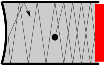
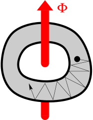
This presentation concerns driven systems, like those illustrated in Fig.​​ 1, whose dynamics is generated by an Hamiltonian that is represented by a matrix that has the generic structure

$$\mathcal{H}_{\mbox{\tiny total}}\ \ =\ \ \mbox{diag}\{E_{n}\}-f(t)\{V_{nm}\}$$ (1)

Here $E_{n}$ are the ordered energy levels of the unperturbed system. Their density $\varrho$[states/energy] is assumed to be roughly uniform. The system is driven by a low frequency stationary driving source $f(t)$. The elements of the perturbation matrix are $V_{nm}$. The induced transitions have rates that are proportional to $|V_{nm}|^{2}$. We define

$$\bm{X}\ \ =\ \ \{|V_{nm}|^{2}\}$$ (2)

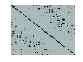
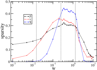
Our interest concerns Hamiltonians that have a “sparse” perturbation matrix. This means that the majority of elements in $\bm{X}$ are small. To be more precise we assume that these elements have a log-wide distribution with a median that is much smaller compared with the average. An example for such matrix is given in Fig.​​ 2, and a typical histogram of the elements is presented in Fig.​​ 3.

Figure 1: Model systems: a Billiard with a moving wall (upper panel), and a Ring with a time dependent magnetic flux (lower panel). The deviation of the Billiard from integrability is quantified by a parameter $u$. It is due to the deformation of the boundary (as in the figure) or due to a deformation of the potential floor (not illustrated). In the lower panel the Ring is regarded as a rectangular-like billiard with periodic boundary conditions in one of its coordinates. In the numerics the Ring has been modeled as a tight binding array of dimensions ${L\times\mathcal{M}}$. In the latter case the non-integrability was due to on-site disorder $W$.

Figure 2: The upper panel is an image of the matrix ${\bm{X}}$ for a billiard very similar in shape to that of Fig.​​ 1. This matrix is ”sparse”. This can be deduced either by inspection, or by looking in the lower panel where the average value $\langle x\rangle$ of the elements (upper curves) is calculated as a function of the distance $\omega$ from the diagonal, and contrasted with the much smaller median values (lower curves). For further details see cqb ; cqc .

Figure 3: Histogram of the in-band elements $x$ of the matrix ${\bm{X}}$ for a rectangular billiard that has deformed potential floor. Different symbols refer to different values of the deformation parameter $u$. The vertical line is the average value of the elements, while the median is roughly at the locations of the peaks. The former unlike the latter is not sensitive to the degree of deformation. For details see kbw .

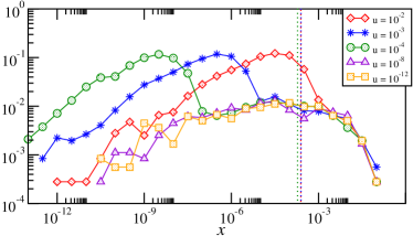
The question that we ask is simple: Given $\bm{X}$, what is the calculation that should be done in order to get the energy absorption rate (EAR). It makes sense that the result should be proportional to some weighted average $\langle\langle\bm{X}\rangle\rangle$ over the matrix elements. Indeed, within the framework of linear response theory (LRT) the Kubo formula is doing just that - a weighted algebraic average.

One should realize that the use of the Kubo formula for EAR calculation can be justified only in the very weak driving limit, provided there is a background “bath” that maintains quasi-equilibrium at any moment. However, if the driving is not very weak, compared with the relaxation, then one should be worried: in order for the system to heat up, it is essential to have connected sequences of transitions, else the system is “stuck”. There is an obvious analogy here with a resistor network calculation: due to the sparsity the energy absorption somewhat resembles a percolation process.

The bottom line of the above considerations is that the algebraic average of Kubo $\langle\langle\bm{X}\rangle\rangle_{a}$, should be replaced by a resistor network average $\langle\langle\bm{X}\rangle\rangle_{s}$, whose value is much smaller if the matrix is “sparse”. This should be regarded as an anomaly in the theory of response: it is an effect that arises upon quantization. Namely, one can characterize the sparsity of $\bm{X}$ by a parameter ${0<s<1}$ that is absent in the classical context, but has a dramatic effect in the quantum analysis.

A few words are in order regarding the literature. We go here beyond the conventional random matrix theory (RMT) perspective of wigner ; bohigas , because we are dealing with “sparse” matrices sparse1 ; sparse2 ; sparse3 ; sparse4 , possibly banded mario1 ; mario2 ; mario3 ; mario4 ; prosen1 ; prosen2 . Our view of LRT follows that of ott1 ; ott2 ; ott3 ; jar1 ; jar2 ; wilk ; WA ; robbins . In the context of Billiards, LRT implies the “Wall formula” wall1 ; wall2 ; wall3 ; frc ; dil ; wlf , while in the context of mesoscopic conductance LRT implies the “Drude formula” kamenev . In both cases one should take into account corrections that are related to correlations and level statistics. The quest for anomalies that cannot be explained by introducing corrections within the framework of LRT, but go beyond LRT, has some history wilk ; WA ; crs ; rsp ; krav1 ; krav2 ; lc . The line of study regarding the anomaly that arises due to “sparsity” is documented in kbr ; bls ; slr ; bld ; kbd ; kbw ; cqb ; cqc , see acknowledgment. The resistor network analysis that is introduced below is inspired by mott ; miller ; AHL ; pollak ; VRHbook ; kbv , but generalizes its scope in a somewhat revolutionary way.

Outline.– We first introduce with more details the model systems of Fig.​​ 1. Then we outline the formalism of the EAR calculation, that is based on a simple Fermi golden rule (FGR) picture. Finally we present results that we have obtained for the dependence of the absorption coefficient or the conductance on the sparsity, where the latter is controlled by the degree of deformation or by the disorder in the system. Two appendices gives extra details on the resistor network calculation and on what we call “resistor network average”.

II The model systems

Assume that we have $N$ non-interacting particles in a “box”. For presentation purpose assume a rectangular-like two dimensional billiard shaped box as in Fig.​​ 1a, or optionally, imposing periodic boundary conditions in once direction, a ring shaped box as in Fig.​​ 1b. The box is slightly deformed: either its walls are slightly curved, or optionally the potential floor is not flat, e.g. due to some scatterer or disorder. The system is driven by a low frequency stationary source. In Fig.​​ 1a the driving is induced by moving a “piston”, while in Fig.​​ 1b it is by varying a magnetic flux through the ring. The Hamiltonian matrix in the unperturbed energy basis takes that form of Eq.​​ (1). In the case of the driven ring we have the identifications

$$f(t) \ \mapsto\ \Phi(t)$$ (3)

$$V_{nm} \ \mapsto\ (e/L)\,v_{nm}$$ (4)

where $\Phi(t)$ is the magnetic flux, and $v_{nm}$ are the matrix elements of the velocity operator. Note that by Faraday law $-\dot{\Phi}$ is the electromotive force (EMF).

The driving induces transitions between energy levels. We assume stationary driving source, and define the its power spectrum as

$${\tilde{S}(\omega)}\ \ =\ \ \mbox{FT}\ {\langle\dot{f}(t)\dot{f}(0)\rangle}$$ (5)

Note that as far as EAR is concerned, it is a non-zero $\dot{f}$ that makes the Hamiltonian time dependent, corresponding to the EMF in the case of the ring. We assume low frequency driving. Accordingly we write

$$\tilde{S}(\omega)\ \ =\ \ 2\pi\overline{|\dot{f}|^{2}}\ \delta_{c}(\omega)$$ (6)

where the prefactor is the RMS value that characterizes the driving intensity, and $\delta_{c}(\omega)$ is a broadened delta function whose line shape reflects the spectral content of the driving.

III The energy absorption rate

The driving induce transitions between energy levels, which implies diffusion in energy space. This diffusion is characterized by a coefficient $D$[energy²/time] for which we would like to have a formula. Assuming that $D$ is known, the EAR is given by the following expression:

$$\mbox{EAR}\ \ =\ \ \mbox{density}\times D$$ (7)

This is a straightforward generalization of Einstein type relations that are discussed in wilk and in greater details in frc . We can call it a diffusion-dissipation relation. What we label in Eq.​​ (7) as “density” stands for the number of particles ($N$) per energy, meaning $N/T$ in the case of a Boltzmann occupation at tempeature $T$, or $\varrho$ in the case of a low temperature Fermi occupation. In the latter case the role of the temperature is overtaken by the Fermi energy, namely ${\varrho\sim N/E_{\mbox{\tiny F}}}$.

What we would like to have, is a theory that allows the calculation of $D$. The formulas that we would like to advertise is

$$D\ \ =\ \ \pi\varrho\ \langle\langle|{V_{nm}}|^{2}\rangle\rangle\ \overline{\dot{f}^{2}}$$ (8)

Depending on the interpretation of $\langle\langle|{V_{nm}}|^{2}\rangle\rangle$ this is the Kubo formula of LRT, or its resistor-network variation. In the latter case we refer to the results as the outcome of semi-linear response theory (SLRT). The latter term indicates that $\langle\langle|{V_{nm}}|^{2}\rangle\rangle_{s}$ unlike $\langle\langle|{V_{nm}}|^{2}\rangle\rangle_{a}$ is a semi-linear rather than linear operation. The derivations of both the LRT and the SLRT variations of Eq.​​ (8) are outlined in the next sections.

In the case of an EMF driven Ring, it is convenient to re-write the EAR formulas Eq.​​ (7) as

$$\mbox{EAR}\ \ =\ \ G\,\overline{\dot{f}^{2}}$$ (9)

where the so-called mesoscopic conductance is given by the expression

$$G\ \ =\ \ \pi\varrho^{2}\ \left(\frac{e}{L}\right)^{2}\ \langle\langle|v_{mn}|^{2}\rangle\rangle$$ (10)

One can regard $G$ as a mesoscopic version of the absorption coefficient, while Eq.​​ (9) can be regarded as the mesoscopic version of Joule law.

IV The Fermi golden rule picture and the Kubo formula

The Hamiltonian in the standard basis is Eq.​​ (1). We can transform it to the adiabatic basis:

$$\tilde{\mathcal{H}}\ \ =\ \ \mbox{diag}\{E_{n}\}-{\dot{f}(t)}\left\{\frac{i{V_{nm}}}{E_{n}-E_{m}}\right\}$$ (11)

The FGR transition rate from $E_{m}$ to $E_{n}$ due to the low frequency noisy driving is:

$$w_{nm}\ \ =\ \ \left|\frac{{V_{nm}}}{E_{n}-E_{m}}\right|^{2}\ \tilde{S}(E_{n}{-}E_{m})$$ (12)

The FGR transitions lead to diffusion in energy space. Assuming that there is a background relaxation process that maintains at any moment quasi-equilibrium with occupation probabilities $p_{n}$ that are the same as in the absence of driving, we get for the driving induced diffusion

$$D\ \ =\ \ \sum_{n}p_{n}\left[\frac{1}{2}\sum_{m}(E_{m}{-}E_{n})^{2}\ w_{mn}\right]$$ (13)

leading to the Kubo formula

$$D\ \ =\ \ \int_{0}^{\infty}{\tilde{C}(\omega)}{\tilde{S}(\omega)}\frac{d\omega}{2\pi}$$ (14)

with the spectral function

$$\tilde{C}(\omega) = \mbox{FT}\ {\langle V(t)V(0)\rangle}$$

$$= \sum_{n}p_{n}\sum_{m}|V_{nm}|^{2}\ 2\pi\delta(\omega-(E_{m}{-}E_{n}))$$

Note that this spectral function reflects the band profile of $\bm{X}$, as defined in Eq.​​ (2), and illustrated in Fig.​​ 2.

It is important to realize that the Kubo formula Eq.​​ (14) is a linear functional of $\tilde{S}(\omega)$. The dependence on the matrix elements of $\bm{X}$ is linear too:

$$D\ \ =\ \ \left[\pi\sum_{n,m}p_{n}|V_{mn}|^{2}\ \delta_{c}(E_{m}{-}E_{n})\right]\ \overline{\dot{f}^{2}}$$ (16)

This can be formally written as Eq.​​ (8) with an implied definition of the weighted algebraic average $\langle\langle|{V_{nm}}|^{2}\rangle\rangle_{a}$.

For completeness we note that in the context of conductance calculation the popular textbook version of the Kubo formula is

$$G=\pi\left(\frac{e}{L}\right)^{2}\sum_{n,m}|v_{mn}|^{2}\ \delta_{{T}}(E_{n}{-}E_{F})\ \delta_{c}(E_{m}{-}E_{n})$$ (17)

This expression is implied by Eq.​​ (16), with averaging over the levels in the vicinity of the Fermi energy. Namely ${p_{n}=\varrho^{-1}\delta_{T}(E_{n}{-}E_{F})}$, where the width of $\delta_{T}()$ is determined by the temperature.

Figure 4: The driving induces transitions between levels $E_{n}$ of a closed system, leading to diffusion in energy space, and hence an associated heating. The diffusion coefficient $D$ can be calculated using a resistor network analogy. Connected sequences of transitions are essential in order to have a non-vanishing result, as in the theory of percolation.

V The calculation of the diffusion coefficient

We would like to consider circumstances in which the driving induced transitions are faster compared with the background relaxation. In such circumstances the occupation probabilities $p_{n}$ are no longer as in equilibrium. For the purpose of analysis we simply neglect the bath, and describe the dynamics by a rate equation

$$\frac{dp_{n}}{dt}=-\sum_{m}w_{nm}(p_{n}-p_{m})$$ (18)

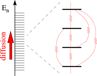
where the rates $w_{nm}$ are determined by Eq.​​ (12). The matrix ${\bm{w}=\{w_{nm}\}}$ can be regarded as a quasi one-dimensional network. See Fig.​​ 4. Optionally one may interpret the rate equation as a probabilistic description of a random walk process, where $w_{nm}$ is the probability to hop from $m$ to $n$ per unit time. The local spreading is described by

$$\mbox{Var}(n)\ \ = \ \ \sum_{n}[w_{n,n_{0}}t]\,(n-n_{0})^{2}$$ (19)

$$\equiv \ \ 2\tilde{D}_{\mbox{\tiny local}}t$$ (20)

It follows that the course-grained spreading should be described by a diffusion equations

$$\frac{\partial p_{n}}{\partial t}\ \ =\ \ \tilde{D}\frac{\partial^{2}}{\partial n^{2}}p_{n}$$ (21)

where $n$ is regarded as a continuous variable. The diffusion equation is formally a continuity equation

$$\frac{\partial p_{n}}{\partial t}\ \ =\ \ -\frac{\partial}{\partial n}I_{n}$$ (22)

where the current is given by Fick’s law:

$$I_{n}\ \ =\ \ -\tilde{D}\frac{\partial}{\partial n}p_{n}$$ (23)

If we have a sample of length $N$ then

$$I\ \ =\ \ -\frac{\tilde{D}}{N}\times[p_{N}-p_{0}]$$ (24)

This shows that $\tilde{D}/N$ is formally like the inverse resistance of the chain: it is the ratio between the current and the “potential difference”. We therefore can use standard recipes of electrical engineering in order to calculate its value. For example, if we have only near-neighbor transitions then “adding connectors in series” implies

$$\frac{\tilde{D}}{N}\ \ =\ \ \left[\sum_{n=1}^{N}\frac{1}{w_{n,n{-}1}}\right]^{-1}$$ (25)

In general we use the notation $\tilde{D}=[[\bm{w}]]$, where the doubled brackets stand for inverse resistivity calculation, as discussed in App.A.

In the above analysis we have assumed unit distance between sites. If the mean level spacing is $\varrho^{-1}$, the expression for the diffusion coefficient should be re-scaled as follows:

$$D\ \ =\ \ \varrho^{-2}[[\bm{w}]]$$ (26)

Recall that the $w_{nm}$ are given by Eq.​​ (12), it follows that

$$D=\varrho^{-2}\left[\left[\left|\frac{{V_{nm}}}{E_{n}-E_{m}}\right|^{2}\ 2\pi\overline{|\dot{f}|^{2}}\delta_{c}(E_{n}{-}E_{m})\right]\right]$$ (27)

leading to Eq.​​ (10), with an implied definition of the resistor network average $\langle\langle|V_{nm}|^{2}\rangle\rangle_{s}$. The definition and the calculation of the latter are further discussed in App.B.

VI The wall formula and beyond

The roughest estimate for the diffusion that is induced by a vibrating wall is known as the “Wall formula” wall1 ; wall2 ; wall3 ; frc ; dil ; wlf . Its original derivation is based on a simple kinetic picture: it is based on the assumption that collisions with the vibrating wall are not correlated. This leads in the two dimensional case frc ; cqc to the result

$$D_{0}\ \ =\ \ \frac{4}{3\pi}\frac{\mathsf{m}^{2}v_{\mbox{\tiny E}}^{3}}{L_{x}}\ {\overline{\dot{f}^{2}}}$$ (28)

where $\mathsf{m}$ is the mass of the particles, and $L_{x}$ is the linear dimension of the box as illustrated in Fig.​​ 1. The result assumes a microcanonical preparation at energy $E$, and we have defined $v_{\mbox{\tiny E}}=[2E/\mathsf{m}]^{1/2}$. If we have a Boltzmann occupation, the expression should be averaged accordingly. If we have low temperature Fermi occupation, what counts in Eq.​​ (7) is the the value at $E=E_{\mbox{\tiny F}}$.

Within the framework of LRT the same result is obtained from the Kubo formula Eq.​​ (14), provided $\tilde{C}(\omega)$ is flat, i.e. provided there are no correlations between collisions. In practice there are correlations leading to ${D=g_{c}D_{0}}$ with $g_{c}$ that can be either smaller or larger than unity depending on the geometry. In the quantum calculation $g_{c}$ is slightly affected by the level spacing statistics.

Within the framework of SLRT one has to calculate the resistor network average of the $\bm{X}$ matrix. If this matrix is sparse, the result becomes very suppressed, leading to ${D=g_{s}g_{c}D_{0}}$, where

$$g_{s}\ \ \equiv\ \ \frac{\langle\langle|V_{nm}|^{2}\rangle\rangle_{s}}{\langle\langle|V_{nm}|^{2}\rangle\rangle_{a}}$$ (29)

We emphasize that $g_{s}$ reflects an anomaly: it depends on the sparsity $s$ of the matrix, a parameter that has no meaning in the classical context. For more details, including RMT analysis of this dependence see kbd .

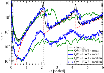
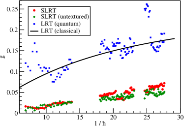
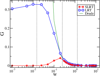
Some numerical results for $g_{c}$ (LRT) and $g=g_{s}g_{c}$ (SLRT) are presented in Fig.​​ 5. The calculation is done with the $\tilde{C}(\omega)$ of Fig.​​ 2. The $\hbar$ dependence of the LRT “classical” result is due to the lower cutoff of the $d\omega$ integral in the Kubo formula Eq.​​ (14), that is sensitive to mean level spacing. If $\tilde{C}(\omega)$ were “flat” the result would not be much sensitive to $\hbar$. As expected the SLRT calculation gives a much smaller result. The effect becomes more conspicuous for smaller deformations, for which the sparsity is “stronger”.

Figure 5: The scaled absorption coefficient $g_{c}$ (LRT) and $g=g_{s}g_{c}$ (SLRT) versus the dimensionless $1/\hbar$ (upper panel), and versus the dimensionless deformation parameter $u$ (lower panel). The input for this analysis is the matrix $\bm{X}$ of Fig.​​ 2. The calculation of each point has been carried out on a $100\times 100$ sub-matrix of $\bm{X}$ centered around the $\hbar$ implied energy $E$. The “untextured” data points are calculated for an artificial random matrices with the same bandprofile and sparsity. The complementary lower panel is oriented to show the small $u$ dependence within an energy window that corresponds to ${1/\hbar\sim 9}$. For further details see cqb ; cqc .

VII The Drude formula and beyond

The EAR by particles that are driven by an oscillating electric field, due to an induced EMF, is very similar problem to that of particles driven by an oscillating wall. Here the simple result that is based on kinetic considerations is known as the “Drude formula”. As in the case of the “Wall formula” it is assumed that scattering events are uncorrelated, leading to the estimate

$$D_{0}\ \ =\ \ \left(\frac{e}{L}\right)^{2}\ v_{\mbox{\tiny E}}\ell\ \ \overline{\dot{\Phi}^{2}}$$ (30)

where $e$ is the charge of the electron, $L$ is the length of the ring, and $\ell$ is the mean free path between collisions. Note that $\mathcal{D}=v_{\mbox{\tiny E}}\ell$ is the spatial diffusion coefficient, while $(e\dot{\Phi}/L)$ is the energy that is gained per circulation. The implied result for the conductance can be written as

$$G_{0}\ \ =\ \ \frac{e^{2}}{2\pi\hbar}\ \mathcal{M}\ \frac{\ell}{L}$$ (31)

where $\mathcal{M}=\mathsf{m}v_{\mbox{\tiny E}}L_{y}/\pi$ is the number of open modes. This way of writing the Drude formula is very illuminating because it reflects Ohm law, and the units are as in the Landauer formula. For clarity we have restored the $\hbar$ in this formula.

Within the framework of LRT, the same result is obtained from the Kubo formula Eq.​​ (14), provided $\tilde{C}(\omega)$ of Eq.​​ (IV) is a Lorentzian that reflects an exponential decay of the velcoity-velocity correlation function. In practice there are extra correlations leading to ${D=g_{c}D_{0}}$ with $g_{c}$ that can be either smaller or larger than unity depending on the geometry. In the quantum calculation $g_{c}$ is slightly affected by the level spacing statistics, and the correction is of order $(\varrho\omega_{c})^{-1}$. This is sometimes regarded as a variation of weak localization corrections kamenev .

Within the framework of SLRT one has to calculate the resistor network average of the matrix $\{|v_{nm}|^{2}\}$. Here one should distinguish between different regimes, depending on the strength $W$ of the disorder. In the Born approximation the mean free path is ${\ell\propto W^{2}}$, while the localization length is ${\ell_{\infty}\approx\mathcal{M}\ell}$. The diffusive regime, where there is no issue of sparsity, requires an intermediate strength of disorder, such that ${\ell\ll L\ll\ell_{\infty}}$. For either stronger or weaker disorder, the matrix $\{|v_{nm}|^{2}\}$ becomes “sparse”. This is because the eigenstates become non-ergodic: either they are localized in real space (for strong disorder) or in mode space (for weak disorder). Note also that for very weak disorder (”clean” ring) each eigenstate occupies a single mode (up to small correction). For detailed analysis that supports the above picture see kbd .

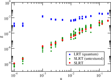
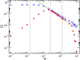
The expectation with regard o the dependence of $G/G_{0}$ on the strength of the disorder is sketched in Fig.​​ 6. Some numerical results for both the LRT and the SLRT conductance are presented in Fig.​​ 7. The calculation is done for a tight binding model. The SLRT result in the Anderson localization regime is completely analogous to the reasoning of variable range hopping mott ; miller ; AHL ; pollak ; VRHbook , as explained in kbv . It should be appreciated that in our approach all regimes are treated on equal footing.

In the ballistic regime, contrary to the Drude expectation, the conductance becomes worse as the disorder is reduced. This looks strange, but can easily be rationalized if we think about the extreme case of no disorder: in the absence of scattering the particle stays all the time in the same mode; hence irreversible diffusive spreading in energy is impossible.

Figure 6: Schematic illustration that sketch the dependence of the DC mesoscopic conductance on the strength of the disorder. It should be regarded as a caricature of Fig.​​ 7. The level width $\Gamma=\hbar\omega_{c}$ affects the so-called weak localization correction in the diffusive regime. In the other two regimes of either weak or strong disorder, the perturbation matrix becomes “sparse” and consequently $G$ is suppressed compared with Drude.

Figure 7: Various measures of sparsity (upper panel), and the mesoscopic conductance (lower panels) as a function of the disorder $W$ in the Ring. The vertical line separate between the clean, ballistic, diffusive and localization regimes. Note that the scaled conductance in arbitrary units equals $\langle\langle|v_{mn}|^{2}\rangle\rangle$. The Drude, the LRT and the SLRT results are displayed in both normal and log scale. We see that in the ballistic regime the SLRT conductance becomes worse as the disorder becomes weaker, in opposition with the Drude expectation. For further details see bld ; kbd

VIII Conclusions

The random matrix approach of Wigner ($\sim 1955$) is based on the observation that in generic circumstances the perturbation can be represented by a random matrix whose elements are taken from a Gaussian distribution. Our interest in this presentation concerned a restricted class of “sparse” systems for which this observation does not hold. In such weak quantum chaos circumstances the elements are characterized by a log-wide distribution. Consequently, the response, and in particular the energy absorption, are similar to a percolation process, and their analysis requires a novel resistor-network approach.

Besides the quantitative issue, the experimental fingerprint of the resistor-network calculation is the implied semi-linearity of the response. In the SLRT regime, i.e. if the driving is the predominant mechanism for transitions between levels, one expects the combined effect of two independent sources to be super-linear, namely,

$$D\big{[}\tilde{S}_{a}(\omega)+\tilde{S}_{b}(\omega)\big{]}\ \ >\ \ D\big{[}\tilde{S}_{a}(\omega)\big{]}+D\big{[}\tilde{S}_{b}(\omega)\big{]}$$ (32)

but still semi-linear $D\big{[}\lambda\tilde{S}(\omega)\big{]}=\lambda\ D\big{[}\tilde{S}(\omega)\big{]}$. We have provides in this presentation two prototype examples where an SLRT anomaly can arise: heating of particles that are trapped in billiards with vibrating walls; and Joule heating of charged carriers that are driven by an induced electro-motive force.

Appendix A The resistor network calculation

In this appendix we explain how the inverse resistivity $G=[[\bm{G}]]$ of a one-dimensional resistor network ${\bm{G}\equiv\{G_{nm}\}}$ is calculated. We use the language of electrical engineering for this purpose. In general this relation is semi-liner rather than linear, namely ${[[\lambda\bm{G}]]=\lambda[[\bm{G}]]}$, but ${[[\bm{A}+\bm{B}]]\neq[[\bm{A}]]+[[\bm{B}]]}$.

There are a few cases where an analytical expression is available. If only near neighbor nodes are connected, allowing ${G_{n,n+1}=g_{n}}$ to be different from each other, then “addition in series” implies that the inverse resistivity calculated for a chain of length $N$ is

$$G\ \ =\ \ \left[\frac{1}{N}\sum_{n=1}^{N}\frac{1}{g_{n}}\right]^{-1}$$ (33)

If $G_{nm}=g_{n-m}$ is a function of the distance between the nodes $n$ and $m$ then it is a nice exercise to prove that “addition in parallel” implies

$$G\ \ =\ \ \sum_{r=1}^{\infty}r^{2}g_{r}$$ (34)

In general an analytical formula for $G$ is not available, and we have to apply a numerical procedure. For this purpose we imagine that each node $n$ is connected to a current source $I_{n}$. The Kirchhoff equations for the voltages are

$$\sum_{m}G_{mn}(V_{n}-V_{m})\ =\ I_{n}$$ (35)

This set of equation can be written in a matrix form:

$$\tilde{\bm{G}}\bm{V}\ =\ \bm{I}$$ (36)

where the so-called discrete Laplacian matrix of the network is defined as

$$\tilde{G}_{nm}=\left[\sum_{n^{\prime}}G_{n^{\prime}n}\right]\delta_{n,m}-G_{nm}$$ (37)

This matrix has an eigenvalue zero which is associated with a uniform voltage eigenvector. Therefore, it has a pseudo-inverse rather than an inverse, and the Kirchhoff equation has a solution if and only if ${\sum_{n}I_{n}=0}$. In order to find the resistance between nodes ${n_{\mbox{\tiny in}}=0}$ and ${n_{\mbox{\tiny our}}=N}$, we set ${I_{0}=1}$ and ${I_{N}=-1}$ and ${I_{n}=0}$ otherwise, and solve for $V_{0}$ and $V_{N}$. The inverse resistivity is ${G=[(V_{0}-V_{N})/N]^{-1}}$.

Appendix B The resistor-newtwork average

We use the notation $\langle\langle\bm{X}\rangle\rangle$ in order to indicate the weighted average value of its elements. First we would like to define the standard algebraic average. It is essential to introduce a weight function that defines the band of interest. In the physical context this function reflects the spectral content of the driving source. Namely, we define $F(r)$ as the normalized version of $\tilde{S}(\omega)$, such that $\sum_{r}F(r)=1$, where ${r=n-m}$ is the energy difference $\omega=E_{n}-E_{m}$ in integer units. The bandwidth in these dimensionless units (${b_{c}=\varrho\omega_{c}}$) it is assumed to be quantum mechanically large ($b_{c}\gg 1$). The algebraic average is defined in the standard way:

$$\langle\langle\bm{X}\rangle\rangle_{a}\ \ =\ \ \frac{1}{N}\sum_{n,m}F(n-m)\ X_{nm}$$ (38)

where $N$ is the size of the matrix, which is assumed to be very large. The algebraic average is a linear operation, meaning that

$$\langle\langle\lambda\bm{X}\rangle\rangle = \lambda\langle\langle\bm{X}\rangle\rangle$$ (39)

$$\langle\langle\bm{X}+\bm{Y}\rangle\rangle = \langle\langle\bm{X}\rangle\rangle+\langle\langle\bm{Y}\rangle\rangle$$ (40)

There are different type of “averages” in the literature, such as the harmonic average, geometric average, and we can also include the median in the same list. All these “averages” are semi-linear operations because only the $\langle\langle\lambda\bm{X}\rangle\rangle=\lambda\langle\langle\bm{X}\rangle\rangle$ property is satisfied for them. Irrespective of the semi-linearity issue any type of average should satisfy the following requirement: if all the elements equal to the same number, then also the average should equal the same number.

In this presentation we highlight a new type of average that we call a resistor-network average:

$$\langle\langle\bm{X}\rangle\rangle_{s}\ \ \equiv\ \ \left[\left[2F(n{-}m)\,\frac{X_{nm}}{(n-m)^{2}}\right]\right]$$ (41)

Writing the expression above as $[[\tilde{w}_{nm}]]$, one should realize that the $\tilde{w}_{nm}$ can be regarded as FGR transition rates. Using Eq.​​ (34) it is not difficult to show that if all the elements $X_{nm}$ are the same number, then also their resistor network average is the same number. While in general

$$\langle\langle\bm{X}\rangle\rangle_{s}\ \ <\ \ \langle\langle\bm{X}\rangle\rangle_{a}$$ (42)

Typically the resistor network average is bounded from below by the median. In order to get a realistic estimate in the case of a “sparse” matrix one can use a generalized variable range hopping scheme that we have developed in kbd .