Consistent modeling of the geodetic precession in Earth rotation

Abstract

A highly precise model for the motion of a rigid Earth is indispensable to reveal the effects of non-rigidity in the rotation of the Earth from observations. To meet the accuracy goal of modern theories of Earth rotation of 1 microarcsecond ($\mu$as) it is clear, that for such a model also relativistic effects have to be taken into account. The largest of these effects is the so called geodetic precession.
In this paper we will describe this effect and the standard procedure to deal with it in modeling Earth rotation up to now. With our relativistic model of Earth rotation (Klioner et al., 2001) we are able to give a consistent post-Newtonian treatment of the rotational motion of a rigid Earth in the framework of General Relativity. Using this model we show that the currently applied standard treatment of geodetic precession is not correct. The inconsistency of the standard treatment leads to errors in all modern theories of Earth rotation with a magnitude of up to 200 $\mu$as for a time span of one century.

1 Introduction

Geodetic precession/nutation is the largest relativistic effect in Earth rotation. This effect has been discovered already a few years after the formulation of General Relativity (de Sitter, 1916) and very early it was recognized to be important for Earth rotation. It results mainly in a slow rotation of a geocentric locally inertial reference frame with respect to remote celestial objects roughly about the ecliptic normal. Due to its relatively large magnitude of about $1.9^{\prime\prime}$ per century, which is $3\times 10^{-4}$ of the general precession, corresponding corrections are used in all standard theories of precession and nutation since the IAU 1980 theory (Seidelmann, 1982).

The standard way to consider geodetic precession in Earth rotation theories up to now was the following: firstly, using purely Newtonian equations, one computed the orientation of the Earth in a geocentric, locally inertial reference frame. To obtain the solution with respect to the kinematically non-rotating Geocentric Celestial Reference System (GCRS) the corrections for geodetic precession were then simply added, as described for example in Bretagnon et al. (1997, Section 8). These corrections can be calculated separately, since they are completely independent of the rotational state of the Earth, e. g. Brumberg et al. (1991).

The purpose of this work is to demonstrate that the standard way of applying the geodetic precession is not correct. After stating the problem in the following Section, we explain shortly our relativistic model of Earth rotation used for this study in Section 3. In Section 4 we describe how the corrections for the geodetic precession can be computed, while in Section 5 two different, but equivalent and correct ways to obtain a GCRS solution are given. In the last section of this paper we compare our solution to published ones and draw concluding remarks.

Throughout the paper we will use the following conventions:

• Lower case Latin indices take the values $1,2,3$.

• Repeated indices imply the Einstein’s summation irrespective of their positions, e. g. $x^{i}y^{i}=x^{1}y^{1}+x^{2}y^{2}+x^{3}y^{3}$

• $\epsilon_{abc}$ is the fully antisymmetric Levi-Civita symbol, defined as $\epsilon_{abc}=(a-b)(b-c)(c-a)/2$.

• Vectors are set boldface and italic: ${\bm{X}}=X^{\,i}$, while matrices are set boldface and upright: ${\bf P}=P^{\,ij}$

• The choice to use index or vector notation for a specific formula is done with regard to readability and clarity.

2 The GCRS and geodetic precession

The Geocentric Celestial Reference System is officially adopted by the IAU to be used to describe physical phenomena in the vicinity of the Earth and, in particular, the rotational motion of the Earth. The GCRS is connected with the Barycentric Celestial Reference System (BCRS) by a generalized version of the Lorentz transformation. This transformation was chosen in such a way that the GCRS spatial coordinates ${\bm{X}}_{K}$ are kinematically non-rotating with respect to the BCRS coordinates, i. e. no additional spatial rotation of the coordinates is involved in the transformation from one system to the other (Soffel et al., 2003).

Since the origin of the GCRS coincides with the geocenter and the Earth is moving in the gravitational field of the Solar system a local inertial frame with spatial coordinates ${\bm{X}}_{D}$ slowly rotates in the GCRS:

$$X^{i}_{D}=R^{\,ij}(T)\,X^{j}_{K}.$$ (1)

Here $R^{\,ij}$ is an orthogonal matrix, the time variable $T$ is the Geocentric Coordinate Time ${\rm TCG}$. Due to this rotation the equations of motion in the GCRS contain a Coriolis force. The locally inertial analogon of the GCRS is called dynamically non-rotating. This rotation between the kinematically non-rotating GCRS and its dynamically non-rotating counterpart is called geodetic precession. The angular velocity of geodetic precession $\bm{\Omega}_{\rm GP}$ is given by

$$\bm{\Omega}_{\rm GP}\approx\frac{1}{c^{2}}\sum_{A}\frac{GM_{A}}{r_{EA}^{3}}\left[\left(\frac{3}{2}\bm{v}_{E}-2\bm{v}_{A}\right)\times\bm{r}_{EA}\right],$$ (2)

where $c$ is the speed of light in the vacuum, $G$ the gravitational constant, $\bm{v}_{A}$ the BCRS velocity of the body $A$ with mass $M_{A}$, $\bm{v}_{E}$ is the velocity of the geocenter, $\bm{r}_{EA}$ the vector from body $A$ to the geocenter and $r_{EA}$ its Euclidean norm. The angular velocity $\bm{\Omega}_{\rm GP}$ corresponds to the orthogonal matrix $R^{\,ij}$ so that the respective kinematical Euler equations read

$$\Omega_{\rm GP}^{a}={1\over 2}\,\varepsilon_{abc}\,R^{\,db}(T)\,{d\over dT}\,R^{\,dc}(T).$$ (3)

This equation can be easily verified by direct substitution of the matrix elements.

3 Model of Earth rotation

A complete and profound discussion of our relativistic model of Earth rotation can be found in Klioner et al. (2001, 2010). For the purposes of this work we neglect all other relativistic effects except for the geodetic precession. In particular, we neglect relativistic torques, relativistic time scales, and relativistic scaling of various parameters. Then, in dynamically non-rotating coordinates ${\bm{X}}_{D}$ the equations of rotational motion of the Earth can be written as

$${d\over dT}\,{\bm{S}}_{D}={\bm{L}}_{D},$$ (4)

$${\bm{S}}_{D}={\bm{S}}_{D}({\bf P}_{D};{\cal A,B,C}),$$ (5)

$${\bm{L}}_{D}={\bm{L}}_{D}({\bf P}_{D};C_{lm},S_{lm};{\bm{x}}_{AD}).$$ (6)

Here ${\bm{L}}_{D}$ is the torque and ${\bm{S}}_{D}$ the angular momentum in the dynamical non-rotating frame and ${\bf P}_{D}$ is a time-dependent orthogonal matrix transforming the coordinates ${\bm{X}}_{D}$ to a terrestrial reference system ${\bm{Y}}$, where the gravitational field of the Earth is constant:

$$Y^{a}=P_{D}^{\,ab}(T)\,X_{D}^{b}.$$ (7)

${\cal A,B,C}$ are the principle moments of inertia of the Earth, $C_{lm},S_{lm}$ are the coefficients of the gravitational field of the Earth in ${\bm{Y}}$ and ${\bm{x}}_{AD}$ are the BCRS coordinates ${\bm{x}}_{A}$ of body A (Sun, Moon, etc.) rotated by the geodetic precession:

$$x^{i}_{AD}=R^{\,ij}(T)\,x^{j}_{A}.$$ (8)

The matrix ${\bf P}_{D}$ can be parametrized by Euler angles $\varphi$, $\psi$ and $\omega$ in the usual way (Bretagnon et al., 1997). Thus, these three angles as functions of time $T$ represent a solution of Eqs. (4)–(6). Note that the only difference between a purely Newtonian solution of Earth rotation and Eqs. (4)–(6) is that the torque should be computed by using rotated positions ${\bm{x}}_{AD}$ of external bodies and not the normal BCRS positions ${\bm{x}}_{A}$. This reflects the fact that the coordinates ${\bm{X}}_{D}$ rotate with respect to the BCRS.

The corresponding equations in the kinematically non-rotating GCRS take the form

$${d\over dT}\,{\bm{S}}_{K}={\bm{L}}_{K}+\bm{\Omega}_{\rm GP}\times{\bm{S}}_{K},$$ (9)

$${\bm{S}}_{K}={\bm{S}}_{K}({\bf P}_{K};{\cal A,B,C};\bm{\Omega}_{\rm GP}),$$ (10)

$${\bm{L}}_{K}={\bm{L}}_{K}({\bf P}_{K};C_{lm},S_{lm};{\bm{x}}_{A}).$$ (11)

The torque ${\bm{L}}_{K}$ is defined by the same functional form as ${\bm{L}}_{D}$, but the coordinates of external bodies are taken directly in the BCRS. Eq. (9) contains an additional Coriolis torque proportional to $\bm{\Omega}_{\rm GP}$. Besides this, the angular momentum ${\bm{S}}_{K}$ in the GCRS explicitly depends on the geodetic precession $\bm{\Omega}_{\rm GP}$. For details of these equations see Klioner et al. (2010) and references therein.

From Eqs. (1) and (7) it is clear, that the solutions of these two sets of equations are related by

$$P^{\,ab}_{K}=P^{\,ac}_{D}\,R^{\,cb}.$$ (12)

4 Computing the geodetic precession

To determine the effect of geodetic precession one has to compute the matrix ${\bf R}$. This can be done by a numerical integration of Eqs. (2)–(3). It should be remarked that care has to be taken how to represent this matrix properly. To avoid the discontinuities that can arise when using the common Euler angles to describe an arbitrary rotation, we decided to use quaternions to represent this matrix. With matrix ${\bf R}$, solution ${\bf P}_{D}$ and Eq. (12) we can calculate the differences $\delta\varphi$, $\delta\psi$ and $\delta\omega$ between the Euler angles $\varphi$, $\psi$ and $\omega$ corresponding to matrix ${\bf P}_{K}$ and those corresponding to ${\bf P}_{D}$.

In the process of computing and verifying the results we have found and corrected a sign error for the correction induced by the geodetic precession for angle $\varphi$ in Bretagnon et al. (1998). Taking this sign error into account the differences between the analytical solution for $\delta\varphi$, $\delta\psi$ and $\delta\omega$ derived by Brumberg et al. (1991) and Bretagnon et al. (1998) and our numerical solution are below 1 $\mu$as. They are shown in Fig. 1.

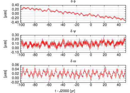
Figure 1: Differences (in $\mu$as) for the analytical solution for geodetic precession derived by Bretagnon et al. (1998) and our numerical solution. The sign error in the SMART solution (Bretagnon et al., 1998) for angle $\varphi$ is corrected here.

The remaining differences are explained by the limited accuracy of the analytical treatment of this effect by the other authors compared to our numerical result.

5 Computing the GCRS solution

According to the equations given in Section 3 there are two ways to compute the matrix ${\bf P}_{K}$ corresponding to the solution of the rotational motion of the Earth with respect to the kinematically non-rotating GCRS:

1. One can numerically integrate Eqs. (4)–(6) and obtain the solution ${\bf P}_{D}$ with respect to dynamically non-rotating coordinates ${\bm{X}}_{D}$. Then one can correct for geodetic precession using the matrix ${\bf R}$ and Eq. (12) to rotate the solution into the GCRS.

2. One can integrate Eqs. (9)–(11) and directly obtain ${\bf P}_{K}$.

Obviously, the initial conditions for Eqs. (4)–(6) and (9)–(11) are again related by (12) taken at the initial epoch.

We have implemented both of the above mentioned possibilities to compute ${\bf P}_{K}$ and verified that the differences in $\varphi$, $\psi$ and $\omega$ computed in the two ways represent only numerical noise at the level of 0.001 $\mu$as and less after 100 years of integration.

The implementation is done in an efficient way. The numerical integration of the matrix ${\bf R}$ runs for example simultaneously with the numerical integration for ${\bf P}_{D}$. The relative running times between a purely Newtonian integration and both ways described above are given in Table 1. Further details on our numerical code and its capabilities can be found for example in Klioner et al. (2008).

Table 1: Relative CPU times for various integrations.

Newtonian case	1.00
Interation of ${\bf P}_{D}$ with rotated ephemeris	1.21
Direct integration of ${\bf P}_{K}$	1.08

A purely Newtonian model differs from Eqs. (4)–(6) only by the positions of the solar system bodies used to compute the torque on the Earth: the Newtonian model uses the BCRS ephemeris directly, while for Eqs. (4)–(6) one has to rotate this ephemeris according to Eq. (8). It is this rotation that has never been considered before in any theory of Earth rotation, which represents the main source of inconsistency in the standard way of taking the geodetic precession into account. The effect of the rotation of the ephemeris on the Euler angles $\varphi$, $\psi$ and $\omega$ is shown in Fig. 2. One finds that the error due to this inconsistency amounts to 200 $\mu$as after 100 years of integration.

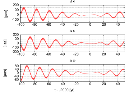
Figure 2: Differences (in $\mu$as) for the Euler angles between a purely Newtonian solution and the correct solution in dynamically non-rotating coordinates. The latter is obtained by using ephemeris data rotated according to Eq. (8).

A summary of the interrelations between the correct solutions for the Earth rotation in dynamically and kinematically non-rotating coordinates as well as Newtonian and “kinematically non-rotating” solution derived in the standard, inconsistent way is given schematically in Fig. 3.

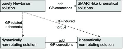
Figure 3: Schematic representation of the differences in the standard and the correct way to treat geodetic precession. “GP” stands for geodetic precession/nutation. Each gray block represents a solution. A solid arrow means: add precomputed geodetic precession/nutation to a solution to get a new one. A dashed arrow means: recompute a solution with indicated change in the torque model.

6 Difference to existing GCRS solutions

The difference between the Euler angles of the GCRS solution obtained in this work and the published kinematically non-rotating SMART solution (Bretagnon et al., 1998) is given in Fig. 4. Analysing the sources of these differences, one can identify three components:

• influence of the rotation of the ephemeris shown in Fig. 2 due to the incorrect treatment of the geodetic precession;

• sign error in the correction for geodetic precession in $\varphi$;

• errors of the analytical SMART solution compared to the more accurate numerical integration, as already discussed in Bretagnon et al. (1998).

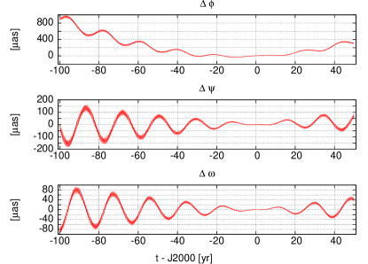
Figure 4: Differences (in $\mu$as) between the published kinematically non-rotating SMART solution and the correct kinematically non-rotating solution derived in this study.

It should be remarked that the above-mentioned inconsistency is not only restricted to the SMART solution, which we used in this study for comparison, but is also contained in the IAU 2000A Precession-Nutation model as described in section 5.5.1 of the IERS Conventions (McCarthy and Petit, 2004). Therefore Fig. 4 allows us to conclude that the existing GCRS solutions for rigid Earth rotation are wrong by 1000 $\mu$as in $\varphi$, 200 $\mu$as in $\psi$ and 100 $\mu$as in $\omega$ within 100 years from J2000. It can be shown that these differences cannot be eliminated by fitting the free parameters of our model, namely the moments of inertia, the initial Euler angles and their time derivatives.

Let us finally note that the effects of non-rigidity in the Earth rotation and the inaccuracies of the corresponding models, e. g. for the atmosphere and oceans, are significantly larger than the effects discussed in this work. Nevertheless to avoid a wrong geophysical interpretation of the observed Earth orientation parameters, the treatment of geodetic precession should be done along the lines presented in this paper.

References

- Bretagnon et al. (1998) Bretagnon, P., Francou, G., Rocher, P., and Simon, J. L. (1998): SMART97: a new solution for the rotation of the rigid Earth, Astron. Astrophys. 329, 329-338.
- Bretagnon et al. (1997) Bretagnon, P., Rocher, P., and Simon, J. L. (1997): Theory of the rotation of the rigid Earth., Astron. Astrophys. 319, 305-317.
- Brumberg et al. (1991) Brumberg, V. A., Bretagnon, P., and Francou, G. (1991): Analytical algorithms of relativistic reduction of astronomical observations. in Journées 1991: Systèmes de Référence Spatio-temporels, pp 141–148.
- de Sitter (1916) de Sitter, W. (1916): Einstein’s theory of gravitation and its astronomical consequences, Mon. Not. R. Astron. Soc. 76, 699-728.
- Klioner et al. (2010) Klioner, S. A., Gerlach, E., and Soffel, M. H. (2010): Relativistic aspects of rotational motion of celestial bodies in S. A. Klioner, P. K. Seidelmann, and M. H. Soffel (eds.), IAU Symposium 261, pp 112–123.
- Klioner et al. (2008) Klioner, S. A., Soffel, M. H., and Le Poncin-Lafitte, C. (2008): Towards the relativistic theory of precession and nutation in Journées 2007: Systèmes de Référence Spatio-temporels, pp 139–142.
- Klioner et al. (2001) Klioner, S. A., Soffel, M. H., Xu, C., and Wu, X. (2001): Earth’s rotation in the framework of general relativity: rigid multipole moments in The Celestial Reference Frame for the Future (Proc. of Journées 2007), N. Capitaine (ed.), Paris Observatory, Paris, pp 232–238.
- McCarthy and Petit (2004) McCarthy, D. D. and Petit, G. (2004): IERS Conventions (2003), IERS Technical Note No.32, BKG, Frankfurt.
- Seidelmann (1982) Seidelmann, P. K. (1982): 1980 IAU Nutation: The Final Report of the IAU Working Group on Nutation, Celest. Mech. Dyn. Astron. 27, 79-106.
- Soffel et al. (2003) Soffel, M. H., Klioner, S. A., Petit, G., Wolf, P., Kopeikin, S. M., Bretagnon, P., Brumberg, V. A., Capitaine, N., Damour, T., Fukushima, T., Guinot, B., Huang, T., Lindegren, L., Ma, C., Nordtvedt, K., Ries, J. C., Seidelmann, P. K., Vokrouhlický, D., Will, C. M., and Xu, C. (2003): The IAU 2000 Resolutions for Astrometry, Celestial Mechanics, and Metrology in the Relativistic Framework: Explanatory Supplement, Astron. J. 126, 2687-2706.