Abstract

An effective method for ultrafast magnetization reversal of nanoclusters is suggested. The method is based on coupling a nanocluster to a resonant electric circuit. This coupling causes the appearance of a magnetic feedback field acting on the cluster, which drastically shortens the magnetization reversal time. The influence of the resonator properties, nanocluster parameters, and external fields on the magnetization dynamics and reversal time is analyzed. The magnetization reversal time can be made many orders shorter than the natural relaxation time. The reversal is studied for both the cases of a single nanocluster as well as for the system of many nanoclusters interacting through dipole forces.

PACS numbers: 75.75.Jn, 75.40.Gb, 75.50.Tt, 75.60.Jk,

1 Introduction

The effect of magnetization reversal in nanomaterials is of considerable importance for various magneto-electronic devices, magnetic recording and storage, and other information processing techniques. The standard way of recording an information bit is to reverse the magnetization by applying a magnetic field antiparallel to the magnetization. From another side, the nanoparticle magnetic moment has to be sufficiently stable, which can be achieved by the use of materials with high magnetic anisotropy. But the latter complicates the process of magnetization reversal. In order to resolve the contradiction between these two requirements, different methods of magnetization reversal have been suggested, as can be inferred from the review articles [1,2].

Magnetization reversals caused by thermal fluctuations and phonon-assisted quantum tunneling are rather slow processes at low temperatures, below the blocking temperature, where nanoclusters exhibit stable magnetization [1,2,3-10]. To make the reversal faster, several methods have been suggested. Thus, one can employ transverse magnetic constant fields [11] or short pulses [12-17], transverse microwave alternating fields at magnetic resonance frequency [18-24], and optical laser pulses [25].

In the present paper, we suggest another method for achieving an ultrafast magnetization reversal of nanoclusters. The method is based on coupling the considered nanocluster with a resonator by placing the cluster into the magnetic coil of an electric circuit. Then the motion of the cluster magnetization produces a magnetic feedback field acting on the cluster. This feedback mechanism essentially accelerates the magnetization reversal. Actually, the effect of the accelerated thermalization of nuclear magnets was proposed by Purcell [26] and considered, using the classical Bloch equations, by Blombergen and Pound [27]. Here we study the magnetization reversal by employing quantum microscopic Hamiltonians typical of strongly anisotropic nanoclusters possessing large spins.

We study magnetic clusters with the effective sizes shorter than the exchange length of atoms composing them, when the magnetic cluster is in a single-domain state and its magnetization can be represented by a large total spin. Such clusters are necessarily of nanosizes, which explains their name of nanoclusters. To avoid complications, due to distributions of particle sizes and shapes, we consider the magnetization dynamics of similar nanoclusters. There are two essentially different cases. One is the magnetization reversal of a single nanocluster. And the other is the magnetization dynamics in an ensemble of nanoclusters interacting through dipolar forces. We study both these limiting cases.

2 Spin Dynamics of Magnetic Nanoclusters

Let us, first, consider a single nanocluster. The typical Hamiltonian of a nanocluster, with the total spin ${\bf S}$, can be written in the form

$$\hat{H}=-\mu_{0}{\bf B}\cdot{\bf S}-D\left(S^{z}\right)^{2}+D_{2}\left(S^{x}\right)^{2}\;,$$ (1)

where $\mu_{0}=-\hbar\gamma_{S}$ is the cluster magnetic moment, $\gamma_{S}\approx 2\mu_{B}/\hbar$ is the gyromagnetic ratio, $\mu_{B}$, Bohr magneton, ${\bf B}$ is the total magnetic field acting on the cluster, $D$ and $D_{2}$ are anisotropy constants. This Hamiltonian reminds the classical Stoner-Wohlfarth model [28,29]. However, we start with the microscopic quantum Hamiltonian (1), where the spin vector is treated as an operator. This will allow us to explicitly define all system parameters and to take into account quantum effects that can be important for the dynamics of nanocluster assemblies.

One usually represents the cluster energy in a reduced form [1,2] with the anisotropy parameters related to $D$ and $D_{2}$ as

$$K=\frac{DS^{2}}{V_{1}}\;,\qquad K_{2}=\frac{D_{2}S^{2}}{V_{1}}\;,$$ (2)

with $V_{1}$ being the single-cluster volume and $S$, the cluster spin value. The second-order magnetic anisotropy is caused by magnetocrystalline anisotropy, shape anisotropy, and surface anisotropy [1,2]. Sometimes, one includes the fourth-order and sixth-order anisotropy. However such higher-order anisotropy terms are usually much smaller than the second-order terms, so their inclusion does not essentially change the overall picture.

The total magnetic field is the sum

$${\bf B}=B_{0}{\bf e}_{z}+H{\bf e}_{x}+B_{1}{\bf e}_{y}$$ (3)

of an external constant magnetic field, generally having the longitudinal, $B_{0}$, and transverse, $B_{1}$, components, and of the resonator feedback field $H$ directed along the axis of the coil, where the cluster is inserted to. The field $B_{0}$ is directed opposite to the initial cluster magnetization. The magnetic field, created by the coil, is described by the Kirchhoff equation. The latter, as is known, defines electric current generated in the coil by varying magnetization. In turn, the current produces magnetic field along the coil axis. The resulting equation for the generated magnetic field $H=H(t)$ can be written [30,31] in the form

$$\frac{dH}{dt}+2\gamma H+\omega^{2}\int_{0}^{t}H(t^{\prime})\;dt^{\prime}=-4\pi\eta\;\frac{dm_{x}}{dt}\;,$$ (4)

in which $\omega$ is the circuit natural frequency, $\gamma$ is the circuit attenuation, $\eta=V_{1}/V_{res}$ is the filling factor, with $V_{res}$ being the volume of the resonant coil, and

$$m_{x}\equiv\frac{\mu_{0}}{V_{1}}\;\langle S^{x}\rangle$$ (5)

is the average magnetization density, corresponding to the mean spin in the direction of the coil axis. Thus, moving spins produce magnetic field that acts back on spins, accelerating their motion.

To write down the equations of motion for the spin operators, it is convenient to introduce several notations. We define the Zeeman frequency

$$\omega_{0}\equiv-\;\frac{\mu_{0}}{\hbar}\;B_{0}=\gamma_{S}B_{0}\;,$$ (6)

the transverse frequency

$$\omega_{1}\equiv-\frac{\mu_{0}}{\hbar}\;B_{1}=\gamma_{S}B_{1}\;,$$ (7)

and the effective transverse field acting on the spin,

$$f\equiv-\;\frac{i}{\hbar}\;\mu_{0}H+\omega_{1}\;.$$ (8)

Then the Heisenberg equations of motion for the spin operators $S^{\pm}=S^{x}\pm S^{y}$ take the form

$$\frac{dS^{-}}{dt}=-i\omega_{0}S^{-}+fS^{z}+i\;\frac{D}{\hbar}\;\left(S^{-}S^{z}+S^{z}S^{-}\right)+i\;\frac{D_{2}}{\hbar}\;\left(S^{x}S^{z}+S^{z}S^{x}\right)\;,$$ (9)

plus its Hermitian conjugate. And the equation for the longitudinal spin becomes

$$\frac{dS^{z}}{dt}=-\;\frac{1}{2}\;\left(f^{*}S^{-}+S^{+}f\right)+\frac{D_{2}}{\hbar}\;\left(S^{x}S^{y}+S^{y}S^{x}\right)\;.$$ (10)

The measurable quantities are the average spin components, such as the reduced transverse component

$$u\equiv\frac{1}{S}\;\langle S^{-}\rangle$$ (11)

and the reduced longitudinal magnetization

$$s\equiv\frac{1}{S}\;\langle S^{z}\rangle\;.$$ (12)

Averaging the equations of motion (9) and (10), we use the decoupling

$$\langle S^{\alpha}S^{\beta}+S^{\beta}S^{\alpha}\rangle=\left(2\;-\;\frac{1}{S}\right)\langle S^{\alpha}\rangle\langle S^{\beta}\rangle\qquad(\alpha\neq\beta)\;,$$ (13)

which preserves the correct behavior for all spins. Thus, for spin one-half it gives exactly zero, because of the anticommutativity of different Pauli matrices, and it becomes asymptotically exact for large spins [32-34]. We also take into account that nanoclusters possess a longitudinal relaxation rate $\gamma_{1}$ that is due to phonon-assisted tunneling and to spin-phonon interactions of the nanocluster with its surrounding.

Let us introduce the longitudinal anisotropy frequency

$$\omega_{D}\equiv(2S-1)\;\frac{D}{\hbar}\;,$$ (14)

the transverse anisotropy frequency

$$\omega_{2}\equiv(2S-1)\;\frac{D_{2}}{\hbar}\;,$$ (15)

the effective anisotropy frequency

$$\omega_{A}\equiv\omega_{D}+\frac{1}{2}\;\omega_{2}\;,$$ (16)

and the effective rotation frequency

$$\Omega\equiv\omega_{0}-\omega_{A}s\;.$$ (17)

Also, let us define the effective field

$$F\equiv f+\frac{i}{2}\;\omega_{2}u^{*}=-\;\frac{i}{\hbar}\;\mu_{0}H+\omega_{1}+\frac{i}{2}\;\omega_{2}u^{*}\;.$$ (18)

Then averaging Eqs. (9) and (10) yields the equations for the transverse spin component,

$$\frac{du}{dt}=-i\Omega u+Fs\;,$$ (19)

plus its complex conjugate, and for the spin magnetization,

$$\frac{ds}{dt}=-\;\frac{1}{2}\left(u^{*}F+F^{*}u\right)-\gamma_{1}(s-\zeta)\;,$$ (20)

where $\zeta$ is the equilibrium magnetization of a cluster.

There exists a large variety of different nanoclusters [1,2,6,35-38], because of which the system parameters can take values in a wide range. Concrete examples will be discussed in the concluding section.

3 Approximate Analysis of Spin Dynamics

The equations of motion (19) and (20) are derived for arbitrary cluster parameters. Their solution can be done numerically. But before we pass to numerical investigation, it is useful to give an approximate qualitative analysis allowing for the better understanding of physics involved. For this purpose, we shall assume that some of the parameters are small as compared to the Zeeman and resonator frequencies.

First, it is possible to show [32-34] that the feedback equation (4) can be represented as the integral equation

$$H=-4\pi\eta\int_{0}^{t}G(t-t^{\prime})\dot{m}_{x}(t^{\prime})\;dt^{\prime}\;,$$ (21)

in which the transfer function is

$$G(t)=\left[\cos(\widetilde{\omega}t)\;-\;\frac{\gamma}{\widetilde{\omega}}\;\sin(\widetilde{\omega}t)\right]\;e^{-\gamma t}\;,$$

with the shifted frequency

$$\widetilde{\omega}\;\equiv\;\sqrt{\omega^{2}-\gamma^{2}}\;,$$

and the source is

$$\dot{m}_{x}=\frac{\mu_{0}S}{2V_{1}}\;\frac{d}{dt}\;\left(u^{*}+u\right)\;.$$

The resonator feedback field efficiently acts on the cluster only when the resonator natural frequency is tuned close to the Zeeman frequency, so that the detuning be small, satisfying the resonance condition

$$\left|\frac{\Delta}{\omega}\right|\ll 1\qquad(\Delta\equiv\omega-\omega_{0})\;.$$ (22)

The effective rotation frequency (17) should also be close to $\omega$, which requires that the anisotropy frequency (16) be also sufficiently small,

$$\left|\frac{\omega_{A}}{\omega}\right|\ll 1.$$ (23)

We assume that all attenuation parameters are smaller than $\omega$, such that

$$\frac{\gamma}{\omega}\ll 1\;,\qquad\frac{\gamma_{1}}{\omega}\ll 1\;.$$ (24)

And let us introduce the parameter playing the role of the feedback rate

$$\gamma_{0}\equiv\pi\eta\;\frac{\mu_{0}^{2}S}{\hbar V_{1}}=\pi\;\frac{\mu_{0}^{2}S}{\hbar V_{res}}\;,$$ (25)

which characterizes the attenuation caused by the coupling between the cluster and resonator.

Under these conditions, the solution to the integral equation (21) can be found by an iterative procedure [32-34], which here gives

$$\mu_{0}H=i\hbar\left(\alpha u-\alpha^{*}u^{*}\right)\;,$$ (26)

where the coupling function, for small detuning, such that $|\Delta|<\gamma$, reads as

$$\alpha=\frac{\gamma\gamma_{0}\Omega}{\gamma^{2}+\Delta^{2}}\;\left(1\;-\;e^{-\gamma t}\right)\;.$$ (27)

Substituting form (26) into Eqs. (19) and (20) results in the equations

$$\frac{du}{dt}=-i\Omega u+\alpha su+\omega_{1}s-s\left(\widetilde{\alpha}u\right)^{*}\;,$$

$$\frac{dw}{dt}=2\alpha sw+\omega_{1}\left(u^{*}+u\right)s-2s{\rm Re}\left(\widetilde{\alpha}u^{2}\right)\;,$$

$$\frac{ds}{dt}=-\alpha w\;-\;\frac{\omega_{1}}{2}\;\left(u^{*}+u\right)-\gamma_{1}(s-\zeta)+{\rm Re}\left(\widetilde{\alpha}u^{2}\right)\;,$$ (28)

in which

$$w\equiv|\;u\;|^{2}\;,\qquad\widetilde{\alpha}\equiv\alpha+\frac{i}{2}\;\omega_{2}\;.$$ (29)

According to inequalities (22) to (24), the variables $w$ and $s$ can be treated as slowly varying in time, while $u$ as a fast variable. The existence of two time scales allows us to invoke the scale separation approach [30,31,39,40] that is a variant of the averaging techniques [41]. Then we solve the equation for $u$, keeping there $w$ and $s$ as quasi-integrals of motion, which gives

$$u=-\;\frac{i\omega_{1}s}{\Omega+i\alpha s}+\left(u_{0}+\frac{\omega_{1}s}{\Omega+i\alpha s}\right)\exp\left\{-i(\Omega+i\alpha s)t\right\}\;,$$ (30)

where $u_{0}\equiv u(0)$. This solution is to be substituted into the equations for the slow variables $w$ and $s$, with averaging their right-hand sides over time, thus, obtaining the equations for the guiding centers of $w$ and $s$.

The scale separation approach is a very powerful method for dealing with a system of many interacting elements, such as the assemblies of spins [30-34] or of quantum dots [42]. However, it requires the use of limitations on the range of the system parameters, such as inequalities (22) to (24). While, in our case, we have derived Eqs. (19) and (20) that are valid for arbitrary parameter values. The latter equations are not difficult to solve numerically. But the present approximate consideration is useful for understanding the following physical points.

The source of creating the resonator feedback field (21) is the motion of the cluster spin, which generates the magnetic field (26) acting back on the spin. The back action is absent at the initial time. The coupling of the cluster spin and the resonator increases with time according to the behavior of the coupling function (27). The transverse spin component (30) oscillates with time with the rotation frequency (17). The initial push to the spin oscillation is done by the transverse field $B_{1}$ entering through the transverse frequency (7). This also requires that the initial magnetization (12) be nonzero. Generally, there is one more source triggering the initial spin motion. These are quantum spin fluctuations that start the spin motion even in the absence of a transverse field, as has been shown for multi-spin systems [30-33]. Such quantum spin fluctuations are especially important for particles with low spins. The input of quantum fluctuations for large spins $S\gg 1$ diminishes as $1/S$, in agreement with Eq. (13). Therefore, in the case of a single nanocluster, these fluctuations can be neglected as soon as the transverse field $B_{1}$ is present. The transverse field, that can be easily regulated, serves as a convenient triggering mechanism for initiating spin motion.

4 Numerical Solution of Evolution Equations

Now we go back to the general evolution equations (19) and (20). For numerical investigation, it is appropriate to pass to dimensionless quantities. To this end, we define the dimensionless feedback field

$$h\equiv-\;\frac{\mu_{0}H}{\hbar\gamma_{0}}=\frac{\gamma_{S}H}{\gamma_{0}}\;.$$ (31)

The effective forces (8) and (18), respectively, become

$$f=i\gamma_{0}h+\omega_{1}\;,\qquad F=i\gamma_{0}h+\frac{i}{2}\;\omega_{2}u^{*}+\omega_{1}\;.$$ (32)

Instead of the complex variable (11), let us use the real components

$$x\equiv\frac{1}{S}\;\langle S^{x}\rangle\;,\qquad y\equiv\frac{1}{S}\;\langle S^{y}\rangle\;,$$ (33)

when

$$u=\frac{1}{S}\;\langle S^{-}\rangle=x-iy\;.$$

And in the following, let us measure time in units of $1/\gamma_{0}$.

With these notations, Eqs. (19) and (20) yield the equations for the spin components:

$$\frac{dx}{dt}=-\omega_{0}y+\omega_{D}ys+\omega_{1}s\;,$$ (34)

$$\frac{dy}{dt}=\omega_{0}x-(\omega_{D}+\omega_{2})xs-hs\;,$$ (35)

$$\frac{ds}{dt}=hy-\omega_{1}x+\omega_{2}xy-\gamma_{1}(s-\zeta)\;.$$ (36)

The feedback equation (4) can be rewritten in the form

$$\frac{d^{2}h}{dt^{2}}+2\gamma\;\frac{dh}{dt}+\omega^{2}h=4\;\frac{d^{2}x}{dt^{2}}\;.$$ (37)

We assume that at the starting moment of time the cluster magnetization is polarized along the axis $z$, which implies the initial spin components

$$x_{0}\equiv x(0)=0\;,\qquad y_{0}\equiv y(0)=0\;,\qquad s_{0}\equiv s(0)=1\;.$$ (38)

And for the initial feedback field we set

$$h_{0}\equiv h(0)=0\;,\qquad\dot{h}_{0}\equiv\dot{h}(0)=0\;,$$ (39)

where the overdot signifies time derivative.

The overall time evolution is described by Eqs. (34) to (37), with the initial conditions (38) and (39). These equations possess the stable stationary solution

$$x^{*}=0\;,\qquad y^{*}=\frac{\omega_{1}\zeta}{\omega_{0}-\omega_{D}\zeta}\;,\qquad s^{*}=\zeta\;,\qquad h^{*}=\dot{h}^{*}=0\;,$$ (40)

that is reached in the relaxation time $T_{1}=1/\gamma_{1}$. The attenuation $\gamma_{1}$ can be defined by the Arrhenius law

$$\gamma_{1}=\gamma_{A}\exp\left(-\;\frac{E_{A}}{k_{B}T}\right)\;,$$

where $E_{A}=\hbar\omega_{A}S$ is the anisotropy barrier. At low temperatures, below the blocking temperature, the attenuation $\gamma_{1}$ is exponentially suppressed, so that the relaxation time $T_{1}$ is very long. However the magnetization reversal can be ultrafast due to the action of the resonator feedback field. In our calculations, we set $\gamma_{1}=10^{-3}$ (in units of $\gamma_{0}$) and take the initial conditions (38) and (39).

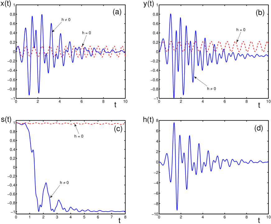
Figure 1: Solutions to the evolution equations: (a) $x=x(t)$; (b) $y=y(t)$; (c) $s=s(t)$; (d) $h=h(t)$ for the parameters $\omega_{0}=\omega=10$, $\omega_{D}=\omega_{1}=\omega_{2}=1,\gamma=1,\gamma_{1}=10^{-3}$. The parameters are measured in units of $\gamma_{0}$ and time, in units of $1/\gamma_{0}$. To emphasize the role of the resonator feedback field, the solutions in the presence of the resonator (solid lines) are compared with those for the case of no resonator (dashed lines).

Figure 1 shows the solutions to the evolution equations (34) to (37), with the initial conditions (38) and (39), as functions of time (in units of $1/\gamma_{0}$) for typical parameters expressed in units of $\gamma_{0}$. The resonator feedback field realizes the magnetization reversal that can be many orders shorter than the relaxation time $T_{1}$. Comparing the behavior in the presence of the resonator and in its absence, we see that in the time scale of $1/\gamma_{0}$ the influence of $\gamma_{1}$ is not noticeable at all.

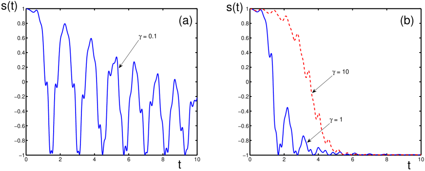
Figure 2: Role of the resonator attenuation. Magnetization as a function of time for the parameters $\omega_{0}=\omega=10,\omega_{D}=\omega_{1}=\omega_{2}=1$ and varying resonator attenuation: (a) $\gamma=0.1$; (b) $\gamma=1$ (solid line) and $\gamma=10$ (dashed line).

Figure 2 demonstrates the influence of the resonator attenuation on the magnetization reversal. Too short $\gamma$ means a large ringing time $1/\gamma$, when the resonator several times exchanges the energy with the cluster, which leads to the oscillations of the magnetization. The optimal value of the resonator attenuation is $\gamma=1$, when the resonator attenuation $\gamma$ coincides with the attenuation $\gamma_{0}$ characterizing the coupling between the resonator and the cluster.

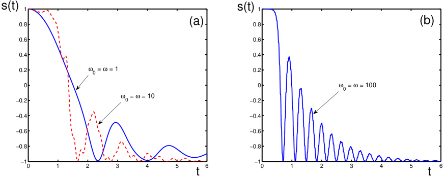
Figure 3: Role of the Zeeman frequency. Magnetization as a function of time for the parameters $\omega_{D}=\omega_{1}=\omega_{2}=1$, $\gamma=1$ and varying Zeeman frequency: (a) $\omega_{0}=\omega=1$ (solid line) and $\omega_{0}=\omega=10$ (dashed line); (b) $\omega_{0}=\omega=100$.

Figure 3 illustrates the role of the Zeeman frequency. The larger the latter, the shorter the reversal time. However too large $\omega_{0}$ leads to many oscillations of magnetization, which is not good, if one aims at the stable reversal.

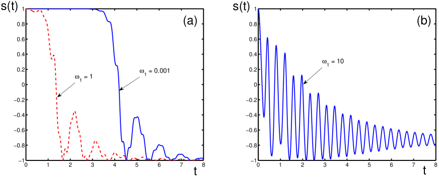
Figure 4: Role of the triggering field. Magnetization as a function of time for the parameters $\omega_{0}=\omega=10$, $\omega_{D}=\omega_{2}=1$, and varying triggering field: (a) $\omega_{1}=0.001$ (solid line) and $\omega_{1}=1$ (dashed line); (b) $\omega_{1}=10$.

Figure 4 shows the influence of the transverse field $B_{1}$ entering through the transverse frequency $\omega_{1}$. The larger the latter, the shorter the reversal time. But too large $\omega_{1}$ results in multiple oscillations, which may be inconvenient for practical purposes.

Figure 5 demonstrates the role of magnetic anisotropy. The anisotropy frequencies that are smaller than the Zeeman frequency do not strongly influence the reversal. But if the anisotropy frequencies are larger than the Zeeman frequency, then the reversal is blocked.

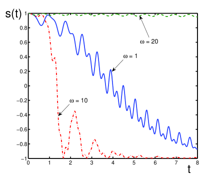
Figure 6: Role of the resonance. Magnetization as a function of time for the parameters $\omega_{0}=10$, $\omega_{D}=\omega_{1}=\omega_{2}=1$, $\gamma=1$, and varying detuning from the resonance, with $\omega=1$ (solid line); $\omega=10$ (dashed-dotted line); $\omega=20$ (dashed line).

Figure 6 shows the importance of the resonance condition. Large detuning from resonance makes the magnetization reversal slower. The larger the detuning, the slower the reversal. The reversal is the fastest when the resonance condition $\omega_{0}=\omega$ is valid.

These figures demonstrate that the coupling to a resonant electric circuit results in the ultrafast magnetization reversal of a single nanocluster, as compared to its natural relaxation time caused by thermal fluctuations and phonon-assisted tunneling. Estimates for typical nanoclusters will be given in the concluding section.

5 System of Nanoclusters with Dipolar Interactions

In the previous sections, we have treated the magnetization reversal of a single nanocluster. An important question is whether such an ultrafast magnetization reversal could be achieved for an ensemble of nanoclusters. The basic difference of the latter case from that of a single cluster is the existence of strong dipolar interactions between the nanoclusters. These dipolar interactions completely suppress coherent spin motion in dephasing time $T_{2}$, so that collective spin rotation, without a resonant feedback, becomes impossible [32-34,43]. One should not confuse the real dipolar interactions between spins with the effective interactions through photon exchange of resonant atoms radiating at optical frequencies. The dipolar spin interactions dephase spin motion, while the atomic interactions through the photon exchange, vice versa, collectivize atomic radiation [44]. Spin motion, of course, also produces electromagnetic radiation that, however, is extremely weak and can never collectivize spins in time shorter than the dephasing time [33,34,43,44]. Self-organized coherent atomic radiation, called superradiance, is the Dicke effect [45]. The principally different collectivization of spin motion by means of a resonator feedback field is what is termed the Purcell effect [26]. The Dicke effect for spin systems is impossible, so that the self-organized coherent spin motion is admissible only through the Purcell effect [32-34,43,44], which necessarily requires the coupling of the spin system with a resonator.

Let us consider a system of $N$ nanoclusters in volume $V$, with the density $\rho\equiv N/V$. The system Hamiltonian reads as

$$\hat{H}=\sum_{j=1}^{N}\hat{H}_{j}+\frac{1}{2}\sum_{i\neq j}^{N}\hat{H}_{ij}\;.$$ (41)

Here the first term is the sum of the single-cluster Hamiltonians

$$\hat{H}_{j}=-\mu_{0}{\bf B}\cdot{\bf S}_{j}-D(S_{j}^{z})^{2}+D_{2}(S_{j}^{x})^{2}\;,$$ (42)

with the cluster spin operators ${\bf S}_{j}$ and the index $j=1,2,\ldots,N$ enumerating the nanoclusters. Aiming at studying the role of the dipolar interactions, we keep in mind similar nanoclusters with close anisotropy parameters and spins $S$. The dipolar interactions are characterized by the Hamiltonian parts

$$\hat{H}_{ij}=\sum_{\alpha\beta}D_{ij}^{\alpha\beta}S_{i}^{\alpha}S_{j}^{\beta}\;,$$ (43)

with the dipolar tensor

$$D_{ij}^{\alpha\beta}=\frac{\mu_{0}^{2}}{r_{ij}^{3}}\;\left(\delta_{\alpha\beta}-3n_{ij}^{\alpha}n_{ij}^{\beta}\right)\;,$$ (44)

in which

$$r_{ij}\equiv|{\bf r}_{ij}|\;,\qquad{\bf n}_{ij}\equiv\frac{{\bf r}_{ij}}{r_{ij}}\;,\qquad{\bf r}_{ij}={\bf r}_{i}-{\bf r}_{j}\;.$$

The resonator feedback field is described by the same Eq. (4), but with

$$m_{x}=\frac{\mu_{0}}{V}\;\sum_{j=1}^{N}\;\langle S_{j}^{x}\rangle\;.$$ (45)

To write the equations of motion in a compact form, we introduce several notations. The dipolar terms are combined into the variables

$$\xi_{i}^{0}\equiv\frac{1}{\hbar}\sum_{j(\neq i)}^{N}\left(a_{ij}S_{j}^{z}+c_{ij}^{*}S_{j}^{-}+c_{ij}S_{j}^{+}\right)\;,\qquad\xi_{i}\equiv\frac{i}{\hbar}\sum_{j(\neq i)}^{N}\left(2c_{ij}S_{j}^{z}\;-\;\frac{1}{2}\;a_{ij}S_{j}^{-}+2b_{ij}S_{j}^{+}\right)\;,$$ (46)

where

$$a_{ij}\equiv D_{ij}^{zz}\;,\qquad b_{ij}\equiv\frac{1}{4}\left(D_{ij}^{xx}-D_{ij}^{yy}-2iD_{ij}^{xy}\right)\;,\qquad c_{ij}\equiv\frac{1}{2}\left(D_{ij}^{xx}-iD_{ij}^{yz}\right)\;.$$ (47)

In the evolution equations, as is well known, there arise pair spin correlators that need to be decoupled for obtaining a closed system of differential equations. For different clusters, we use the semiclassical decoupling

$$\langle S_{i}^{\alpha}S_{j}^{\beta}\rangle=\langle S_{i}^{\alpha}\rangle\langle S_{j}^{\beta}\rangle\qquad(i\neq j)\;,$$ (48)

supplemented by the account of quantum spin correlations yielding the appearance of the dephasing term $\gamma_{2}$. And the spin correlators for different components of the same cluster, similar to Eq. (13), are decoupled as

$$\langle S_{j}^{\alpha}S_{j}^{\beta}+S_{j}^{\beta}S_{j}^{\alpha}\rangle=\left(2\;-\;\frac{1}{S}\right)\langle S_{j}^{\alpha}\rangle\langle S_{j}^{\beta}\rangle\qquad(\alpha\neq\beta)\;,$$ (49)

in order to retain the correct limiting expressions for spin one-half and large spins [32-34]. The angle brackets, as earlier, imply statistical averaging over the initial statistical operator. This type of spin decoupling will lead to the appearance of the expressions

$$\xi_{0}\equiv\frac{1}{N}\sum_{j=1}^{N}\;\langle\xi_{j}^{0}\rangle\;,\qquad\xi\equiv\frac{1}{N}\sum_{j=1}^{N}\;\langle\xi_{j}\rangle\;.$$ (50)

As we see, the consideration of an ensemble of magnetic nanoclusters with dipolar interactions is essentially more complicated than that of a single nanocluster, treated in the previous sections.

6 Magnetization Reversal in Ensemble of Nanoclusters

The quantities of interest are the average spin components, for which it is convenient to introduce, instead of Eqs. (11) and (12), the relative transverse component

$$u\equiv\frac{1}{SN}\sum_{j=1}^{N}\;\langle S_{j}^{-}\rangle$$ (51)

and the relative longitudinal component

$$s\equiv\frac{1}{SN}\sum_{j=1}^{N}\;\langle S_{j}^{z}\rangle\;.$$ (52)

The effective force acting on a cluster spin, instead of Eq. (18), now is

$$F=-\;\frac{i}{\hbar}\;\mu_{0}H+\omega_{1}+\frac{i}{2}\;\omega_{2}u^{*}+\xi\;.$$ (53)

Writing down the equations of motion for the spin operators and averaging them [46], we come to the evolution equations for the mean spin components (51) and (52) in the form

$$\frac{du}{dt}=-i(\Omega+\xi_{0}-i\Gamma_{2})u+Fs\;,\qquad\frac{ds}{dt}=-\;\frac{1}{2}\left(u^{*}F+F^{*}u\right)-\gamma_{1}(s-\zeta)\;,$$ (54)

where

$$\Gamma_{2}=\gamma_{2}\left(1-s^{2}\right)\;,\qquad\gamma_{2}=\frac{\rho\mu_{0}^{2}S}{\hbar}=\rho\hbar\gamma_{S}^{2}S\;.$$ (55)

Equations (54) for a nanocluster system replace Eqs. (19) and (20) for a single cluster. These equations are to be considered together with Eq. (4) for the resonator feedback field, with

$$m_{x}=\frac{1}{2}\;\rho\mu_{0}S(u^{*}+u)\;.$$ (56)

Instead of the feedback rate (25) for a single cluster, for $N$ clusters, we now have

$$\gamma_{0}(N)=\pi N\;\frac{\mu_{0}^{2}S}{\hbar V_{res}}=\pi\eta\rho\hbar\gamma_{S}^{2}S\;.$$ (57)

And instead of the coupling function (27), we get

$$\alpha(N)=g\gamma_{2}(1-As)\left(1-e^{-\gamma t}\right)\;,$$ (58)

with the dimensionless coupling parameter

$$g\equiv\frac{\gamma\omega_{0}\gamma_{0}(N)}{\gamma_{2}(\gamma^{2}+\Delta^{2})}$$ (59)

and the effective anisotropy parameter

$$A\equiv\frac{\omega_{A}}{\omega_{0}}=\frac{2\omega_{D}+\omega_{2}}{2\omega_{0}}\;.$$ (60)

Notice that, for $\pi\eta\sim 1$, the feedback rate (57) is of order of $\gamma_{2}$. Under good resonance, with a small detuning $\Delta\sim 0$, the coupling parameter (59) is $g\sim\omega_{0}/\gamma$.

The system of equations (54) and (21) can be solved numerically, either directly, as has been done for magnetic molecules [47], or invoking the averaging techniques [39,40], when fast oscillations are averaged out, so that the resulting curves are smoothed. Both these methods give close results. The averaging techniques provide more physically transparent description of the initial stage of spin motion, showing that this motion starts with stochastic spin fluctuations caused by nonsecular terms of dipolar interactions. Thus, dipolar interactions play at the initial stage the positive role of a triggering mechanism initiating spin motion, while at the later stage they play the negative role, by destroying the coherence of spin rotation.

In Fig. 7, we show the results of numerical calculations, involving the averaging techniques, for the time dependence of the reduced spin polarization (52) for different system parameters. Time is measured in units of $\gamma_{2}^{-1}$ and all frequencies, in units of $\gamma_{2}$. The realistic value for the anisotropy parameter (60) is taken as $A=0.1$. It is worth emphasizing that for $\gamma_{2}>\omega_{1}$, dipolar interactions initiate spin dynamics so that $\omega_{1}$ plays a minor role. In order to stress the triggering role of the dipolar interactions, the transverse frequency is set to zero, $\omega_{1}=0$. Analogously to Eqs. (38), the initial conditions are

$$w_{0}\equiv w(0)=0\;,\qquad s_{0}\equiv s(0)=1\;,$$

where $w=|u|^{2}=x^{2}+y^{2}$. The figure shows that ultrafast magnetization reversal happens also in a system of nanoclusters interacting through dipolar forces. Even more interesting is the fact that the dipolar interactions play the role of a triggering mechanism starting spin dynamics. The magnetization reversal is realized during the time of order $1/g\gamma_{2}=T_{2}/g$, which, for $g>1$ is shorter that the dephasing time $T_{2}=1/\gamma_{2}$. Hence it is feasible to find the system parameters, when dipolar interactions do not disturb the coherence of spin motion, provided the sample is coupled to a resonator. Without the latter, the Purcell effect does not exist and the ultrafast magnetization reversal is impossible.

7 Discussion

We have suggested a method for realizing an ultrafast magnetization reversal of nanoclusters. The possibility of such a fast reversal is important for a number of applications, e.g., for the functioning of various magneto-electronic devices, spintronics, magnetic recording and storage, and other information processing techniques [48-50]. The idea of the method is based on the coupling of the nanocluster with a resonant electric circuit. This is easily achievable by placing the nanoclusters inside a magnetic coil. Then the motion of the nanocluster magnetic moment produces electric current in the circuit, which creates magnetic field acting back on the cluster magnetization. This feedback field of the resonator accelerates the magnetization reversal. The reversal time can be made many orders shorter than the natural relaxation time.

First, we have considered a single nanocluster, which makes it possible to avoid complications due to distributions of particle sizes, shapes, spin values, and so on, which could arise in the case of an assembly of many nanoclusters. In the latter case, the basic complication is the necessity of taking into account dipole interactions between the clusters. All these additional problems are avoided when dealing with a single cluster.

The case of an ensemble of nanoclusters, interacting through dipolar forces is also analyzed. The ultrafast magnetization reversal is feasible for this case as well. The reversal occurs during the time shorter than the dipole dephasing time, because of which dipolar interactions do not destroy coherent spin motion that is responsible for the ultrafast reversal. Even more, dipolar interactions are useful at the initial stage, when they trigger spin dynamics.

To give the feeling of typical values for the characteristic parameters, let us make estimates for some nanoclusters. Actually, the family of magnetic nanoclusters is very wide and these can display rather different properties [1-3,51-54]. To be concrete, let us keep in mind the values typical of Co, Fe, and Ni nanoclusters. The coherence radius for these clusters, below which they are in a single-domain state and can display coherent rotation of magnetization is $R_{coh}\sim 10$ nm. The standardly formed clusters have the radii $R\sim 1-3$ nm. The corresponding cluster volume is $V_{1}\sim 10^{-20}$ cm³. A cluster contains about $N_{1}\sim 10^{3}$ atoms. The atomic density in a cluster is $\rho_{1}\sim 10^{23}$ cm^-3. The cluster spin is proportional to the number of atoms in the cluster, hence $S\sim 10^{3}$, that is, the magnetic moment is of the order $10^{3}\mu_{B}$. The magnetic anisotropy parameters (2) are $K_{1}\sim K_{2}\sim 10^{6}$ erg/cm³. The fourth-order anisotropy is much smaller, $K_{4}\sim 10^{5}$ erg/cm³. This, for the anisotropy parameters of Hamiltonian (1), gives $D\sim D_{2}\sim 10^{-20}$ erg. And for the fourth-order anisotropy, this would make $D_{4}\sim 10^{-27}$ erg.

These values, for the anisotropy frequencies (14) to (16) yield $\omega_{D}\sim\omega_{2}\sim\omega_{A}\sim 10^{10}$ Hz. This corresponds to the anisotropy field $B_{A}\equiv\omega_{A}/\gamma_{S}\sim 10^{3}$ G. The Zeeman frequency, for the magnetic field $B_{0}\sim 1$ T is $\omega_{0}\sim 10^{11}$ Hz. Note that the present day facilities allow for the generation of magnetic fields as high as about $100$ T [55]. The feedback rate (25) is $\gamma_{0}\sim 10^{10}$ s^-1. This rate provides the reversal time $t_{rev}\sim 1/\gamma_{0}\sim 10^{-10}$ s.

The blocking temperature, below which thermally activated reversals are exponentially suppressed is $T_{B}\sim 10-40$ K. The typical prefactor in the Arrhenius law is $\gamma_{A}\sim 10^{9}-10^{11}$ s^-1. The anisotropy energy barrier in the Arrhenius law is $E_{A}\sim 10^{-14}$ erg. This gives the anisotropy temperature $E_{A}/k_{B}\sim 100$ K. The resulting relaxation time $T_{1}\equiv 1/\gamma_{1}$, below the blocking temperature, is rather long. Thus, even at the temperature $T=10$ K, we have $T_{1}\sim 10^{-5}$ s. At the temperature $T=5$ K, one has $T_{1}\sim 0.1$ s. And for temperature $T=1$ K, the thermal reversal time is astronomically large, being $T_{1}\sim 10^{34}$ s. But, coupling the nanocluster to a resonator, produces a very short reversal time $t_{rev}\sim 10^{-10}$ s, independently of the value $T_{1}$. The reversal time could be made shorter by choosing the appropriate types of nanoclusters and resonator properties.

As has been explained above, the spin relaxation in the system of nanoclusters, which would be caused by the photon exchange between different spins is negligible [33,34,43,44]. The corresponding radiation width is

$$\gamma_{rad}=\frac{2\omega^{3}\mu_{0}^{2}S}{3\hbar c^{3}}=\frac{2\omega^{3}}{3\rho c^{3}}\;\gamma_{2}\;.$$

For the typical density of nanoclusters $\rho\sim 10^{20}$ cm^-3, the spin of a cluster $S\sim 10^{3}$, and frequency $\omega\sim 10^{11}$ Hz, we get $\gamma_{rad}\sim 10^{-8}$ s^-1, which is much smaller than the dipolar width $\gamma_{2}\sim 10^{10}$ s^-1. Therefore the relaxation time, due to the photon exchange between spins, $t_{rad}=1/\gamma_{rad}\sim 10^{8}$ s $\sim 10$ years, is enormously larger than the dipolar dephasing time $T_{2}\sim 10^{-10}$ s. This confirms that the photon exchange mechanism plays no role in the spin relaxation, that is, the Dicke effect for spin systems does not exist. But the ultrafast magnetization reversal is completely due to the Purcell effect.

The typical density of an ensemble of clusters is $\rho\sim 10^{20}$ cm^-3. With the natural dipolar width $\gamma_{2}\sim 10^{10}$ s^-1, the dephasing time is $T_{2}\sim 10^{-10}$ s. As is seen in Fig. 7, the reversal time can be an order shorter than the dephasing time, being $t_{rev}\sim 10^{-11}$ s.

Concluding, by coupling nanoclusters to a resonant electric circuit, it is possible to realize ultrafast magnetization reversal for single nanoclusters as well as for assemblies of nanoclusters. For such nanoclusters as Fe, Co, or Ni, the reversal time can be made as short as $10^{-11}$ s.

Acknowledgement

The authors acknowledge financial support from the Russian Foundation for Basic Research.

Figure Captions

Fig. 1. Solutions to the evolution equations: (a) $x=x(t)$; (b) $y=y(t)$; (c) $s=s(t)$; (d) $h=h(t)$ for the parameters $\omega_{0}=\omega=10$, $\omega_{D}=\omega_{1}=\omega_{2}=1$, $\gamma=1,\gamma_{1}=10^{-3}$. The parameters are measured in units of $\gamma_{0}$ and time, in units of $1/\gamma_{0}$. To emphasize the role of the resonator feedback field, the solutions in the presence of the resonator (solid lines) are compared with those for the case of no resonator (dashed lines).

Fig. 2. Role of the resonator attenuation. Magnetization as a function of time for the parameters $\omega_{0}=\omega=10$, $\omega_{D}=\omega_{1}=\omega_{2}=1$, and varying resonator attenuation: (a) $\gamma=0.1$; (b) $\gamma=1$ (solid line) and $\gamma=10$ (dashed line).

Fig. 3. Role of the Zeeman frequency. Magnetization as a function of time for the parameters $\omega_{D}=\omega_{1}=\omega_{2}=1$, $\gamma=1$, and varying Zeeman frequency: (a) $\omega_{0}=\omega=1$ (solid line) and $\omega_{0}=\omega=10$ (dashed line); (b) $\omega_{0}=\omega=100$.

Fig. 4. Role of the triggering field. Magnetization as a function of time for the parameters $\omega_{0}=\omega=10$, $\omega_{D}=\omega_{2}=1$, and varying triggering field: (a) $\omega_{1}=0.001$ (solid line) and $\omega_{1}=1$ (dashed line); (b) $\omega_{1}=10$.

Fig. 5. Role of the anisotropy. Magnetization as a function of time for the parameters $\omega_{0}=\omega=10$, $\omega_{1}=1,\gamma=1$, and varying anisotropy frequencies $\omega_{D}=\omega_{2}=1$ (dashed-doted line); $\omega_{D}=\omega_{2}=10$ (solid line); $\omega_{D}=\omega_{2}=15$ (dashed line).

Fig. 6. Role of the resonance. Magnetization as a function of time for the parameters $\omega_{0}=10$, $\omega_{D}=\omega_{1}=\omega_{2}=1$, $\gamma=1$, and varying detuning from the resonance, with $\omega=1$ (solid line); $\omega=10$ (dashed-dotted line); $\omega=20$ (dashed line).

Fig. 7. Magnetization reversal in the system of nanoclusters with dipolar interactions. The system parameters are $\gamma_{1}=10^{-3}$, $\Delta=0$, $A=0.1$, $\omega_{1}=0$. Time is measured in units of $T_{2}\equiv 1/\gamma_{2}=10^{-10}$ s, and the frequencies, in units of $\gamma_{2}$. Other parameters are: $\gamma=10$, $\omega_{0}=\omega=1000$, $g=100$ (solid line); $\gamma=1$, $\omega_{0}=\omega=100$, $g=100$ (dashed-dotted line); $\gamma=10$, $\omega_{0}=\omega=100$, $g=10$ (dashed line). The shown functions of time are: (a) coherence intensity $w(t)$; (b) reduced magnetization $s(t)$.

Figure 5: Role of the anisotropy. Magnetization as a function of time for the parameters $\omega_{0}=\omega=10$, $\omega_{1}=1$, $\gamma=1$, and varying anisotropy frequencies $\omega_{D}=\omega_{2}=1$ (dashed-doted line); $\omega_{D}=\omega_{2}=10$ (solid line); $\omega_{D}=\omega_{2}=15$ (dashed line).

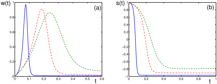
Figure 7: Magnetization reversal in the system of nanoclusters with dipolar interactions. The system parameters are $\gamma_{1}=10^{-3}$, $\Delta=0$, $A=0.1$, $\omega_{1}=0$. Time is measured in units of $T_{2}\equiv 1/\gamma_{2}=10^{-10}$ s, and the frequencies, in units of $\gamma_{2}$. Other parameters are: $\gamma=10$, $\omega_{0}=\omega=1000$, $g=100$ (solid line); $\gamma=1$, $\omega_{0}=\omega=100$, $g=100$ (dashed-dotted line); $\gamma=10$, $\omega_{0}=\omega=100$, $g=10$ (dashed line). The shown functions of time are: (a) coherence intensity $w(t)$; (b) reduced magnetization $s(t)$.

References

- [1] W. Wernsdorfer, Adv. Chem. Phys. 118, 99 (2001).
- [2] J. Ferré, Topics Appl. Phys. 83, 127 (2002).
- [3] B. Barbara, L. Thomas, F. Lionti, I. Chiorescu, and A. Sulpice, J. Magn. Magn. Mater. 200, 167 (1999).
- [4] W. Wernsdorfer, E.B. Orozco, B. Barbara, A. Benoit, and D. Mailly, Physica B 280, 264 (2000).
- [5] R.H. Koch, G. Grinstein, G.A. Keefe, Y. Lu, P.L. Throuilloud, and W.J. Gallagher, Phys. Rev. Lett. 84, 5419 (2000).
- [6] S. Takagi, Macroscopic Quantum Tunneling (Cambridge University, Cambridge, 2002).
- [7] G.F. Goya, F.C. Fonseca, R.F. Jardim, R. Muccillo, N.L. Carreno, E. Longo, and E.R. Leite, J. Appl. Phys. 93, 6531 (2003).
- [8] F. Luis, J. Bartolomé, F. Petroff, L.M. Garcia, A. Vaures, and J. Carrey, J. Appl. Phys. 93, 7032 (2003).
- [9] F. Luis, F. Petroff, and J. Bartolomé, J. Phys. Condens. Matter 16, 5109 (2004).
- [10] S. Krause, G. Herzog, T. Stapelfeldt, L. Berbil-Bautista, M. Bode, E.Y. Vedmedenko, and R. Wiesendanger, Phys. Rev. Lett. 103, 127202 (2009).
- [11] Y.B. Bazaliy and A. Stankiewicz, Appl. Phys. Lett. 98, 142501 (2011).
- [12] H.C. Siegmann, E.L. Garwin, C.Y. Prescott, J. Heidmann, D. Mauri, D. Weller, R. Allenspach, W. Weber, J. Magn. Magn. Mater. 151, 8 (1995).
- [13] O.S. Kolotov, A.P. Krasnozhon, and V.A. Pogozhev, Phys. Solid State 40, 277 (1998).
- [14] C.H. Back, R. Allenspach, W. Weber, S.S. Parkin, D. Weller, E.L. Garwin, and H.C. Siegmann, Science 285, 864 (1999).
- [15] H.W. Schumacher, C. Chappert, R.C. Sousa, P.P. Freitas, and J. Miltat, Phys. Rev. Lett. 90, 017204 (2003).
- [16] S.J. Gamble, M.H. Burkhardt, A. Kashuba, R. Allenspach, S.S. Parkin, H.C. Siegmann, and J. Stöhr, Phys. Rev. Lett. 102, 217201 (2009).
- [17] A. Sukhov and J. Berakdar, Phys. Rev. B 79, 134433 (2009).
- [18] C. Thirion, W. Wernsdorfer, and D. Mailly, Nature Mater. 2, 524 (2003).
- [19] S.I. Denisov, T.V. Lyutyy, P. Hänggi, and K.N. Throhidou, Phys. Rev. B 74, 104406 (2006).
- [20] P.M. Pimentel, B. Leven, B. Hillebrands, and H. Grimm, J. Appl. Phys. 102, 063913 (2007).
- [21] C. Nistor, K. Sun, Z. Wang, M. Wu, C. Mathieu, and M. Hadley, Appl. Phys. Lett. 95, 012504 (2009).
- [22] S. Li, B. Livshitz, H.N. Bertram, E.E. Fullerton, and V. Lomakin, J. Appl. Phys. 105, 07B909 (2009).
- [23] T. Yoshioka, T. Nozaki, T. Seki, M. Shiraishi, T. Shinjo, Y. Suzuki, and Y. Uehara, Appl. Phys. Express 3, 013002 (2010).
- [24] S.V. Titov, P.M. Déjardin, H.E. Mrabti, and Y.P. Kalmykov, Phys. Rev. B 82, 100413 (2010).
- [25] C.D. Stanciu, F. Hansteen, A.V. Kimel, A. Kirilyuk, A. Tsukamoto, A. Itoh, and T. Rasing, Phys. Rev. Lett. 99, 047601 (2007).
- [26] E.M. Purcell, Phys. Rev. 69, 681 (1946).
- [27] N. Bloembergen and R.V. Pound, Phys. Rev. 95, 8 (1954).
- [28] E.C. Stoner and E.P. Wohlfarth, Phil. Trans. Roy. Soc. London A 240, 599 (1948).
- [29] A. Thiaville, J. Magn. Magn. Mater. 182, 5 (1998).
- [30] V.I. Yukalov, Phys. Rev. Lett. 75, 3000 (1995).
- [31] V.I. Yukalov, Phys. Rev. B 53, 9232 (1996).
- [32] V.I. Yukalov, Laser Phys. 12, 1089 (2002).
- [33] V.I. Yukalov and E.P. Yukalova, Phys. Part. Nucl. 35, 348 (2004).
- [34] V.I. Yukalov, Phys. Rev. B 71, 184432 (2005).
- [35] D.J. Sellmyer and R. Skomski, eds. Advanced Magnetic Nanostructures (Springer, Berlin, 2006).
- [36] J.P. Liu, E. Fullerton, O. Guttfleisch, and D.J. Sellmyer, eds. Nanoscale Magnetic Materials and Applications (Springer, Berlin, 2009).
- [37] J.S. Miller and D. Gatteschi, Chem. Soc. Rev. 40, 3065 (2011).
- [38] J.S. Miller, Chem. Soc. Rev. 40, 3266 (2011).
- [39] V.I. Yukalov, Laser Phys. 3, 870 (1993).
- [40] V.I. Yukalov and E.P. Yukalova, Phys. Part. Nucl. 31, 561 (2000).
- [41] N.N. Bogolubov and Y.A. Mitropolsky, Asymptotic Methods in the Theory of Nonlinear Oscillations (Gordon and Breach, New York, 1961).
- [42] V.I. Yukalov and E.P. Yukalova, Phys. Rev. B 81, 075308 (2010).
- [43] V.I. Yukalov and E.P. Yukalova, Laser Phys. Lett. 2, 302 (2005).
- [44] V.I. Yukalov, Laser Phys. Lett. 2, 356 (2005).
- [45] R.H. Dicke, Phys. Rev. 93, 99 (1954).
- [46] V.I. Yukalov and E.P. Yukalova, Laser Phys. Lett. 8, 804 (2011).
- [47] V.I. Yukalov, V.K. Henner, and P.V. Kharebov, Phys. Rev. B 77, 134427 (2008).
- [48] F. Troiani and M. Affronte, Chem. Soc. Rev. 40, 3119 (2011).
- [49] S. Sanvito, Chem. Soc. Rev. 40, 3336 (2011).
- [50] V.I. Yukalov and D. Sornette, Laser Phys. Lett. 6, 833 (2009).
- [51] R.H. Kodama, J. Magn. Magn. Mater. 200, 359 (1999).
- [52] G.C. Hadjipanayis, J. Magn. Magn. Mater. 200, 373 (1999).
- [53] M. Jamet, W. Wernsdorfer, C. Thirion, V. Dupuis, P. Mélinon, A. Pérez, and D. Maily, Phys. Rev. B 69, 024401 (2004).
- [54] G.F. Goya and M.P. Morales, J. Metast. Nanocryst. Mater. 20, 673 (2004).
- [55] M. Motokawa, Rep. Prog. Phys. 67, 1995 (2004).