Giant Monopole Resonances and nuclear incompressibilities studied for the zero-range and separable pairing interactions.

Abstract

Background:

Following the 2007 precise measurements of monopole strengths in tin isotopes, there has been a continuous theoretical effort to obtain a precise description of the experimental results. Up to now, there is no satisfactory explanation of why the tin nuclei appear to be significantly softer than ²⁰⁸Pb.

Purpose:

We determine the influence of finite-range and separable pairing interactions on monopole strength functions in semi-magic nuclei.

Methods:

We employ self-consistently the Quasiparticle Random Phase Approximation on top of spherical Hartree-Fock-Bogolyubov solutions. We use the Arnoldi method to solve the linear-response problem with pairing.

Results:

We found that the difference between centroids of Giant Monopole Resonances measured in lead and tin (about 1 MeV) always turns out to be overestimated by about 100%. We also found that the volume incompressibility, obtained by adjusting the liquid-drop expression to microscopic results, is significantly larger than the infinite-matter incompressibility.

Conclusions:

The zero-range and separable pairing forces cannot induce modifications of monopole strength functions in tin to match experimental data.

I Introduction

The incompressibility of infinite nuclear matter as well as of finite nuclei has been studied in a number of theoretical papers and reviews. In the classic review by Blaizot [Bla80] the connection between the finite-nucleus incompressibility and centroid of the Giant Monopole Resonance (GMR) was shown. This relation allows us to study incompressibility of nuclei through microscopic calculations of the monopole excitation spectra. It also brings us the possibility to directly compare theoretical results with experimental data. For examples, see the measurements presented in Refs. [You99] ; [Li07] ; [Li10] .

In Ref. [Pie10] , it was shown that the self-consistent models that succeed in reproducing the GMR energy in the doubly-magic nucleus ²⁰⁸Pb systematically overestimate the GMR energies in the tin isotopes. In spite of many studies related to the isospin [Sag07] ; [Pea10] ; [Cen10] , surface [Sha09] , and pairing [Civ91] ; [Li08a] ; [Nik08a] ; [Tse09] ; [Kha09a] ; [Kha09b] ; [Kha10] influence on the nuclear incompressibility, to date there is no theoretical explanation of the question ”Why is tin so soft?” [Pie07] ; [Pie10] . For an excellent recent review of the subject matter we refer the reader to Ref. [Li10] .

Studies in Refs. [Kha09a] ; [Kha09b] were restricted to the effect of zero-range pairing interaction. In the present paper we focus on a different kind of pairing force, namely, we implement the finite-range, fully separable, translationally invariant pairing interaction of the Gaussian form [Dug04] ; [Tia09] ; [Nik10] , together with the general phenomenological quasilocal energy density functional in the ph-channel [Car08e] . We have performed calculations for all particle-bound semi-magic nuclei starting from $Z=8$ or $N=8$, up to $Z=82$ or $N=126$. The ground-state properties were explored within the Hartree-Fock-Bogolyubov (HFB) method, whereas the monopole excitations were calculated by using the Quasiparticle Random Phase Approximation (QRPA) within the Arnoldi iteration scheme [Toi10] . For the numerical solutions, we used an extended version of the code HOSPHE [Car10d] .

The paper is organized as follows. In Secs. II and III, we briefly outline the Arnoldi method to solve the QRPA equations and present the separable pairing interaction, respectively. In Sec. IV, we discuss the nuclear incompressibility, including its theoretical description, definitions in finite and infinite nuclear matter, and relations to monopole resonances. Then, our results are shown and discussed in Sec. V and conclusions are given in Sec. VI, whereas the Appendix presents numerical tests of the approach.

II QRPA method

In the present study, we solve the QRPA equations by using the iterative Arnoldi method, implemented in Ref. [Toi10] . It provides us with an extremely efficient and fast way to solve the QRPA equations. The QRPA equations are well known [RS80] ; [Bla86] and have been recently reviewed in the context of the finite amplitude method [Avo11] . Therefore, here we only give a brief resumé of basic equations, by presenting their particularly useful and compact form.

Basic dynamical variables of the QRPA method are given by the generalized density matrix ${\cal R}$,

$${\cal R}=\begin{pmatrix}\rho&\kappa\\ \kappa^{+}&1-\rho^{T}\end{pmatrix}=\begin{pmatrix}V^{*}V^{T}&V^{*}U^{T}\\ U^{*}V^{T}&U^{*}U^{T}\end{pmatrix},$$ (1)

corresponding to mean-field Hamiltonian ${\cal H}=\partial{\cal E}/\partial{\cal R}$,

$${\cal H}=\begin{pmatrix}h-\lambda&\Delta\\ \Delta^{+}&-h^{*}+\lambda\end{pmatrix}.$$ (2)

The standard HFB equations that define amplitudes $U$ and $V$ read

$$\begin{pmatrix}h-\lambda&\Delta\\ \Delta^{+}&-h^{*}+\lambda\end{pmatrix}\begin{pmatrix}U&V^{*}\\ V&U^{*}\end{pmatrix}=\begin{pmatrix}U&V^{*}\\ V&U^{*}\end{pmatrix}\begin{pmatrix}E&0\\ 0&-E\end{pmatrix}$$ (3)

where the diagonal matrix $E$ contains positive quasiparticle energies. Then the quasiparticle ($\chi$) and quasihole ($\varphi$) states are given by columns of eigen-vectors:

$$\varphi:=\begin{pmatrix}V^{*}\\ U^{*}\end{pmatrix},\hskip 56.9055pt\chi:=\begin{pmatrix}U\\ V\end{pmatrix},$$ (4)

that is,

$${\cal H}\varphi=-\varphi E,\hskip 56.9055pt{\cal H}\chi=\chi E.$$ (5)

The vibrational time-dependent HFB state $|\Psi(t)\rangle$,

$$|\Psi(t)\rangle=|\Psi\rangle+\mbox{e}^{i\omega t}|\tilde{\Psi}\rangle,$$ (6)

where $|\tilde{\Psi}\rangle$ is a small-amplitude correction, leads to the time-dependent density matrix,

$${\cal R}(t)={\cal R}+\mbox{e}^{i\omega t}\tilde{\cal R}+\mbox{e}^{-i\omega t}\tilde{\cal R}^{+}$$ (7)

and time-dependent mean field ${\cal H}(t)$,

$${\cal H}(t)={\cal H}+\mbox{e}^{i\omega t}\tilde{\cal H}+\mbox{e}^{-i\omega t}\tilde{\cal H}^{+}.$$ (8)

After a linearization of fields in the time-dependent Hamiltonian, one obtains the QRPA equations in a simple form,

$$-\hbar\omega\tilde{\cal R}=[{\cal H},\tilde{\cal R}]+[\tilde{\cal H},{\cal R}].$$ (9)

In this approach, states in Eq. (6) play a role of Kohn-Sham-like wave functions, which serve the purpose of generating generalized density matrices ${\cal R}(t)$ only. Neither $|\Psi\rangle$ represents a correct ground state of the system nor $|\tilde{\Psi}\rangle$ represents that of an excited vibrational state. However, the amplitude $\tilde{\cal R}$, which constitutes the fundamental degree of freedom of the QRPA method, does represent a fair approximation to the transition density matrix between both states of the system. It then allows for calculating matrix elements of arbitrary one-body operators between the ground state and vibrational state, which is the primary goal of the QRPA approach.

Equation (9) constitutes the base for our solution of the QRPA equations in terms of the iterative Arnoldi method. Indeed, since the mean-field amplitude $\tilde{\cal H}$ depends linearly on the density amplitude $\tilde{\cal R}$, Eq. (9) constitutes an eigen-equation determining $\tilde{\cal R}$ and $\hbar\omega$. However, the matrix to be diagonalized, that is the QRPA matrix, does not have to be explicitly determined. To obtain the entire QRPA strength function, it is enough to start from a pivot amplitude and repeatedly act on it with the expression on the right-hand side [Toi10] . In each iteration, one only has to calculate the mean-field amplitude $\tilde{\cal H}$ corresponding to the current density amplitude $\tilde{\cal R}$, which is an easy task. The pivot can be freely chosen to optimally suit the calculation. It can for example be random, a QRPA eigen-phonon or be constructed from an external field. In this work we construct the pivot from the monopole transition operator. This approach is fundamentally different than that used within the FAM of Ref. [Avo11] , where an external field is used throughout the calculation and Eq. (9) has to be iterated for all values of frequencies $\omega$.

Since both stationary (${\cal R}^{2}={\cal R}$) and time-dependent, (${\cal R}^{2}(t)={\cal R}(t)$) density matrices are projective, the QRPA amplitude $\tilde{\cal R}$ has vanishing matrix elements between the quasihole and between the quasiparticle states, that is,

$$\varphi^{+}\tilde{\cal R}\varphi=\chi^{+}\tilde{\cal R}\chi=0.$$ (10)

Therefore, $\tilde{\cal R}$ is solely defined through the antisymmetric amplitude matrices $\tilde{Z}$ and $\tilde{Z}^{\prime+}$ defined as

$$\tilde{Z}=-\tilde{Z}^{T}=\chi^{+}\tilde{\cal R}\varphi,$$

$$\tilde{Z}^{\prime+}=-\tilde{Z}^{\prime*}=\varphi^{+}\tilde{\cal R}\chi.$$ (11)

Explicitly, amplitudes $\tilde{Z}$ and $\tilde{Z}^{\prime+}$ read

$$\tilde{Z} = U^{+}\tilde{\rho}V^{*}+U^{+}\tilde{\kappa}U^{*}+V^{+}\tilde{\kappa}^{\prime+}V^{*}-V^{+}\tilde{\rho}^{T}U^{*},$$

$$\tilde{Z}^{\prime+} = V^{T}\tilde{\rho}U+V^{T}\tilde{\kappa}V+U^{T}\tilde{\kappa}^{\prime+}U-U^{T}\tilde{\rho}^{T}V.$$ (12)

Within such a formalism, the QRPA equations (9) can be expressed as

$$-\hbar\omega\tilde{Z} = E\tilde{Z}+\tilde{Z}E+\tilde{W},$$

$$\hbar\omega\tilde{Z}^{\prime+} = E\tilde{Z}^{\prime+}+\tilde{Z}^{\prime+}E+\tilde{W}^{\prime+},$$ (13)

where the field amplitudes $\tilde{W}$ and $\tilde{W}^{\prime+}$ are defined as

$$\tilde{W}=-\tilde{W}^{T}=\chi^{+}\tilde{\cal H}\varphi,$$

$$\tilde{W}^{\prime+}=-\tilde{W}^{\prime*}=\varphi^{+}\tilde{\cal H}\chi,$$ (14)

or explicitly,

$$\tilde{W} = U^{+}\tilde{h}V^{*}+U^{+}\tilde{\Delta}U^{*}+V^{+}\tilde{\Delta}^{\prime+}V^{*}-V^{+}\tilde{h}^{T}U^{*},$$

$$\tilde{W}^{\prime+} = V^{T}\tilde{h}U+V^{T}\tilde{\Delta}V+U^{T}\tilde{\Delta}^{\prime+}U-U^{T}\tilde{h}^{T}V.$$ (15)

We can also invert Eq. (12) and obtain transition densities $\tilde{\rho}$, $\tilde{\kappa}$, and $\tilde{\kappa}^{\prime+}$ expressed in terms of amplitudes $\tilde{Z}$ and $\tilde{Z}^{\prime+}$, that is,

$$\tilde{\rho}=U\tilde{Z}V^{T}+V^{*}\tilde{Z}^{\prime+}U^{+},$$

$$\tilde{\kappa}=U\tilde{Z}U^{T}+V^{*}\tilde{Z}^{\prime+}V^{+},$$

$$\tilde{\kappa}^{\prime+}=V\tilde{Z}V^{T}+U^{*}\tilde{Z}^{\prime+}U^{+}.$$ (16)

Finally, we can reduce the above QRPA formalism to spherical symmetry used in the present study. Then, the vibrating amplitude of Eq. (6) has good angular-momentum quantum numbers $JM$, that is, $|\tilde{\Psi}\rangle\equiv|\tilde{\Psi}^{JM}\rangle$ and hence all the QRPA amplitudes pertain to the given preselected channel $JM$, while the ground state $|\Psi\rangle$ is spherical. As a consequence, as dictated by the angular-momentum algebra, only specific spherical single-particle states are coupled by the QRPA amplitudes, which can be expressed through the Wigner-Eckart theorem and reduced matrix elements as

$$\!\!\!\!\tilde{X}^{JM}_{\alpha jm,\alpha^{\prime}j^{\prime}m^{\prime}} \!\!=\!\! \frac{1}{\sqrt{2j+1}}C^{jm}_{j^{\prime}m^{\prime}JM}\langle\psi_{\alpha j}||\tilde{X}^{J}||\psi_{\alpha^{\prime}j^{\prime}}\rangle,$$ (17)

where $\tilde{X}$ stands for amplitudes $\tilde{\rho}$ or $\tilde{h}$, and

$$\!\!\!\!\!\!\!\!\tilde{X}^{JM}_{\alpha jm,\alpha^{\prime}j^{\prime}m^{\prime}} \!\!=\!\! \frac{(-1)}{\sqrt{2J+1}}C^{JM}_{jmj^{\prime}m^{\prime}}\langle\psi_{\alpha j}||\tilde{X}^{J}||\psi_{\alpha^{\prime}j^{\prime}}\rangle,$$ (18)

$$\!\!\!\!\!\!\!\!\tilde{X}^{\prime}{}^{+JM}_{\alpha jm,\alpha^{\prime}j^{\prime}m^{\prime}} \!\!=\!\! \frac{(-1)^{J-M}}{\sqrt{2J+1}}C^{J,-M}_{jmj^{\prime}m^{\prime}}\langle\psi_{\alpha j}||\tilde{X}^{\prime}{}^{+J}||\psi_{\alpha^{\prime}j^{\prime}}\rangle,$$ (19)

where $\tilde{X}$ stands for amplitudes $\tilde{\kappa}$, $\tilde{\Delta}$, $\tilde{Z}$, or $\tilde{W}$. In these expressions, we have used the standard quantum numbers $\alpha jm$ of spherical single-particle states.

Spurious QRPA mode appears in the $0^{+}$ QRPA calculations. In a self-consistent full QRPA diagonalization, the spurious mode decouples from the physical QRPA modes and appears at zero energy. In the Arnoldi method, this separation does not happen unless we make the full Arnoldi diagonalization, which usually is not feasible.

To prevent the mixing of physical QRPA excitations with the spurious $0^{+}$ mode, before the Arnoldi iteration we create the spurious-mode QRPA amplitudes and its associated conjugate-state (boost-mode) QRPA amplitudes. The spurious $0^{+}$ mode amplitudes follow from the particle number operator and have the form,

$$\tilde{P}^{00} = U^{+}V^{*},\quad\tilde{P}^{\prime+00}=V^{T}U.$$ (20)

The $0^{+}$ boost mode is generated by making an additional HFB calculation whose chemical potentials $\lambda_{\tau}$ and average particle numbers are slightly shifted from the ground state values, producing a perturbed state $|{\rm HFB}_{2}\rangle$. The boost-mode amplitudes are calculated by using Thouless theorem as,

$$\tilde{R}^{00}_{\alpha jm,\alpha^{\prime}j^{\prime}m^{\prime}} = \frac{\langle{\rm HFB}_{2}|a^{+}_{\alpha jm}a^{+}_{\alpha^{\prime}j^{\prime}m^{\prime}}|{\rm HFB}\rangle}{\langle{\rm HFB}_{2}|{\rm HFB}\rangle}$$ (21)

$$= \bigl{(}{\tilde{V}}{\tilde{U}}^{-1}\bigr{)}_{\alpha jm,\alpha^{\prime}j^{\prime}m^{\prime}},$$

$$\tilde{R}^{{}^{\prime}+00}_{\alpha jm,\alpha^{\prime}j^{\prime}m^{\prime}} = \frac{\langle{\rm HFB}|a_{\alpha^{\prime}j^{\prime}m^{\prime}}a_{\alpha jm}|{\rm HFB}_{2}\rangle}{\langle{\rm HFB}|{\rm HFB}_{2}\rangle}$$ (22)

$$= \bigl{(}{\tilde{V}}{\tilde{U}}^{-1}\bigr{)}^{*}_{\alpha jm,\alpha^{\prime}j^{\prime}m^{\prime}},$$

where we used the standard transformation matrices from one quasiparticle basis to another [RS80] ,

$${\tilde{V}} = U^{T}V_{2}+V^{T}U_{2},$$ (23)

$${\tilde{U}} = U^{+}U_{2}+V^{+}V_{2}.$$ (24)

Gram-Schmidt orthogonalization is used to keep during the Arnoldi iteration the Krylov-space basis vectors orthogonal to the spurious and boost modes, that is, each Krylov-space basis vector is orthogonalized against ${\tilde{P}}$ and ${\tilde{R}}$. The orthogonalization procedure is described in detail in Ref. [Toi10] . For the semi-magic nuclei considered here, we only vary the particle number of the nucleon species that has non-vanishing pairing correlations.

III Separable Pairing Interaction

The separable finite-range pairing interaction for neutrons ($\tau=n$) and protons ($\tau=p$) that we use in this study is defined as [Tia09]

$$\hat{V}_{\tau}(\bm{r}_{1}s_{1},\bm{r}_{2}s_{2};\bm{r}^{\prime}_{1}s^{\prime}_{1},\bm{r}^{\prime}_{2}s^{\prime}_{2})$$ (25)

$$= -G_{\tau}\delta(\bm{R}-\bm{R}^{\prime})P(r)P(r^{\prime})\frac{1}{2}(1-\hat{P}_{\sigma}),$$

where $\bm{R}=(\bm{r}_{1}+\bm{r}_{2})/2$ denotes the centre of mass coordinate, $\bm{r}=\bm{r}_{1}-\bm{r}_{2}$ is the relative coordinate, $r=|\bm{r}|$, $\hat{P}_{\sigma}$ is the standard spin-exchange operator, and function $P(r)$ is a sum of $m$ Gaussian terms,

$$P(r)=\frac{1}{m}\sum_{i=1}^{m}\frac{1}{(4\pi a_{i}^{2})^{3/2}}\mbox{e}^{-\frac{r^{2}}{4a_{i}^{2}}}.$$ (26)

Coupling constants $G_{\tau}$ define the pairing strengths for neutrons and protons.

For such a pairing interaction, the pairing energy acquires a fully separable form, which in spherical symmetry reads

$$E_{\text{pair}}^{\text{sep}} = -\frac{1}{2}\sum_{NJ\tau}G_{\tau}\Bigl{(}\sum_{\mu\nu}V_{\mu\nu}^{NJ}\langle\psi_{\mu}||\kappa^{\prime+J}_{\tau}||\psi_{\nu}\rangle\Bigr{)}$$ (27)

$$\hskip 42.67912pt\times\Bigl{(}\sum_{\mu^{\prime}\nu^{\prime}}V_{\mu^{\prime}\nu^{\prime}}^{NJ}\langle\psi_{\mu^{\prime}}||\kappa^{J}_{\tau}||\psi_{\nu^{\prime}}\rangle\Bigr{)},$$

and depends on the reduced matrix elements of the pairing densities $\kappa_{\tau}$ and $\kappa^{\prime+}_{\tau}$ between the single-particle wave functions $\psi_{\mu}(\bm{r})$ for $\mu$ denoting the set of spherical harmonic-oscillator (HO) quantum numbers $n_{\mu}l_{\mu}j_{\mu}$. The interaction matrix elements $V_{\mu\nu}^{NJ}$ are defined as

$$V_{\mu\nu}^{NJ} = \sqrt{(4\pi)(2J+1)(2j_{\mu}+1)(2j_{\nu}+1)}\begin{Bmatrix}l_{\mu}&l_{\nu}&J\\ \frac{1}{2}&\frac{1}{2}&0\\ j_{\mu}&j_{\nu}&J\end{Bmatrix}$$ (28)

$$\times M^{NJn0}_{n_{\mu}l_{\mu}n_{\nu}l_{\nu}}\frac{2^{1/4}}{b^{3/2}}\sqrt{\frac{\pi^{1/2}(2n+1)!}{2(2^{n}n!)^{2}}}\frac{1}{m}\sum_{i=1}^{m}\frac{1}{(4\pi a_{i}^{2})^{3/2}}$$

$$\times \Bigl{(}\frac{2a_{i}^{2}b^{2}}{1+a_{i}^{2}b^{2}}\Bigr{)}^{3/2}\Bigl{(}\frac{1-a_{i}^{2}b^{2}}{1+a_{i}^{2}b^{2}}\Bigr{)}^{n},$$

where $2n=2n_{\mu}+l_{\mu}+2n_{\nu}+l_{\nu}-2N-J$, $M^{N\lambda n0}_{n_{\mu}l_{\mu}n_{\nu}l_{\nu}}$ are the standard Talmi-Moshinski coefficients [Bar66] , and $b=\sqrt{m\omega/\hbar}$ denotes the HO constant.

IV Nuclear Incompressibility

The isoscalar incompressibility of infinite nuclear matter is defined by the well-known formula [Bla80]

$$K_{\infty}=9\rho^{2}\frac{\mbox{d}^{2}}{\mbox{d}\rho^{2}}\Bigl{(}\frac{E}{A}\Bigr{)}_{\rho=\rho_{nm}},$$ (29)

where $\rho_{nm}$ is the saturation density of nuclear matter. Of course, $K_{\infty}$ cannot be directly measured; however, by using Eq. (29) it can be calculated from theoretical equation of state $E(\rho)$ or it can be indirectly estimated from measurements of monopole excitations of finite nuclei.

The incompressibility of finite nucleus, $K_{A}$, is defined by its scaling-model relation [Str82] to the centroid of the giant monopole resonance (GMR), $E_{\text{GMR}}$, as

$$E_{\text{GMR}}=\sqrt{\frac{\hbar^{2}K_{A}}{m\langle r^{2}\rangle}}$$ (30)

where $\langle r^{2}\rangle$ is the average square radius of the nucleus. Eq. (30) is derived under the assumption that most of the monopole strength is concentrated within one dominant peak, see Ref. [Bla80] . However, often the monopole giant resonances consist of more than one dominant peak. The reliability of the scaling-model was also challenged in, e.g., Ref.[Nis85] . Therefore, we want to emphasize that extracting the incompressibility $K_{A}$ from the GMR centroid in Eq. (30) is only approximative and model-dependent. For this reason, we pay attention to analyze not only the nuclear incompressibilities, but also directly the GMR centroids.

The centroid of the GMR can be extracted from its strength function as the ratio of the first and zero moments, that is,

$$E_{\text{GMR}}=\frac{m_{1}}{m_{0}}.$$ (31)

There exist several alternative ways to extract $E_{\text{GMR}}$ through different moments of the strength function, such as $E_{\text{GMR}}=\sqrt{m_{1}/m_{-1}}$ or $E_{\text{GMR}}=\sqrt{m_{3}/m_{1}}$. However, they are more sensitive to details of the strength function and thus less appropriate for studies of the incompressibility.

In analogy to the Weizsäcker formula for the nuclear masses, one can introduce [Bla80] a similar relation for nuclear incompressibilities,

$$K_{A} = K_{V}+K_{S}A^{-1/3}+(K_{\tau}+K_{S,\tau}A^{-1/3})\frac{(N-Z)^{2}}{A^{2}}$$ (32)

$$+K_{C}\frac{Z^{2}}{A^{4/3}}\ .$$

Similarly as in the liquid-drop (LD) model, we refer to $K_{V}$, $K_{S}$, $K_{\tau}$, $K_{S,\tau}$, and $K_{C}$ as the volume, surface, symmetry, surface-symmetry, and Coulomb incompressibility parameters, respectively. By adjusting these parameters to the incompressibilities $K_{A}$, calculated in finite nuclei from Eqs. (30) and (31), we can obtain an estimate of the infinite-matter incompressibility as $K_{\infty}\simeq K_{V}$.

V Results

In our study we performed a set of calculations for semi-magic nuclei starting from $Z=8$ or $N=8$ and ending with $Z=82$ or $N=126$. The ground states properties were calculated within the HFB method by using the code HOSPHE [Car10d] , whereas the monopole strength functions were obtained by implementing in the same code the QRPA method within the Arnoldi iterative method [Toi10] .

We decided to use two different Skyrme functionals – SLy4 [Cha98] and UNEDF0 [Kor10b] . Both of them were tuned (among other observables) to reproduce the main properties of the infinite nuclear matter. In particular, they correspond to the same value of nuclear incompressibility (29) of $K_{\infty}=230$ MeV and differ in their values of the effective mass of $m^{*}/m=0.70$ and 1.11 for SLy4 and UNEDF0, respectively.

The present study is focused on comparing incompressibilities obtained with two different pairing interactions, namely, the standard zero-range force, $V_{\tau}(\bm{r},\bm{r}^{\prime})=-V_{0\tau}\delta(\bm{r}-\bm{r}^{\prime})$, and separable force presented in Sec. III. To make the comparison meaningful, we adjusted the strength parameters, $G_{\tau}$ and $V_{\tau}$, so as to obtain for both forces very similar neutron (proton) pairing gaps in $Z=50$ isotopes ($N=50$ isotones). The resulting gaps roughly correspond to the experimental odd-even mass staggering along the $Z=50$ and $N=50$ chains of nuclei. Theoretical pairing gaps, $\Delta_{n}$ and $\Delta_{p}$, were determined as in Ref. [Dob96] , namely,

$$\Delta_{\tau}=\frac{\mbox{Tr}^{\prime}(\rho_{\tau}\Delta_{\tau})}{\mbox{Tr}\rho_{\tau}}$$ (33)

where $\mbox{Tr}A=\sum_{k}A_{kk}$ and $\mbox{Tr}^{\prime}A=\sum_{k>0}A_{k\bar{k}}$. For the separable pairing, in Eq. (26) we used only one Gaussian term with $a_{1}=0.66$ fm.

In this way, in the calculations we used the separable-force strength parameters of $G_{n}=631$ and 473 MeV fm³ ($G_{p}=647$ and 521 MeV fm³) for the SLy4 and UNEDF0 functionals, respectively, and similarly, for the zero-range force: $V_{n}=195$ and 126 MeV fm³ ($V_{p}=221$ and 157 MeV fm³). All calculated neutron and proton pairing gaps are shown in Figs. 1 and 2, respectively. One can see that the results obtained for both pairing forces are fairly similar. The HFB iterations were carried out using a linear mixing of densities from the current and previous iteration defined by a constant mixing parameter [Car10d] . With this recipe, for some of the nuclei, the HFB iterations did not end in converged solutions. Such cases were excluded from the analysis of pairing properties and the subsequent QRPA calculations.

We note here that no energy cut-off is needed for calculations using the separable force, and thus in our calculations the entire HO basis up to $N_{0}=20$ shells was used, see Appendix A. On the other hand, for the zero-range force we used the cut-off energy of 60 MeV applied within the two-basis method [Gal94] ; [Sch12] .

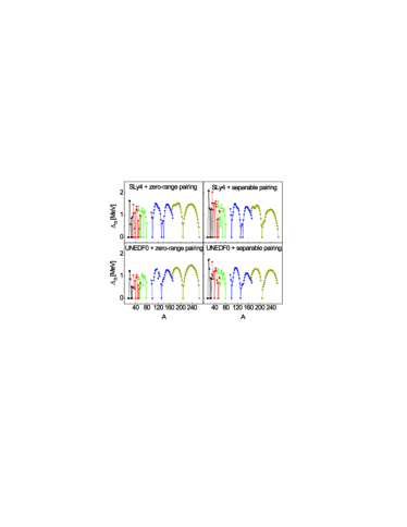
Figure 1: (Color online) Neutron pairing gaps in the $Z=8$, 20, 28, 50, and 82 isotopes (see the legend shown in Fig. 4). Upper and lower panels show results obtained for the SLy4 and UNEDF0 functionals, respectively. Left and right panels show results obtained for the zero-range and separable pairing, respectively.

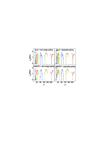
Figure 2: (Color online) Same as in Fig. 1 but for the proton gaps in the $N=8$, 20, 28, 50, 82, and 126 isotones (see the legend shown in Fig. 5).

In Fig. 3 we compare our QRPA results with raw experimental data obtained in Ref. [Li10] . In this work, a Lorentzian fit to data was performed in the region of energies of 10.5–20.5 MeV, and the experimental values of ${m_{1}}/{m_{0}}$ were determined from the corresponding fitted curve (its moments were calculated for energies from zero to infinity). In determining our theoretical values of ${m_{1}}/{m_{0}}$, we also perform the integration in the entire energy domain. We have checked that the integration of theoretical curves in the fixed region of 10.5–20.5 MeV does not bring meaningful results, because, in the wide region of masses studied here, the GMR peaks move too much, and extend beyond the above narrow range of energies. Our QRPA strength functions were obtained from the discrete Arnoldi strength distributions by using the smoothing methods explained in Ref. [Toi10] . We also note that in our QRPA calculations, the high-energy shoulder of the strength function is not obtained, cf. discussion in Ref. [Li10] .

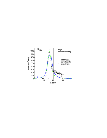
Figure 3: (Color online) The QRPA monopole strength function in ¹¹²Sn (solid line) compared to raw experimental data [Li10] and Lorentzian fit to data (dashed line) performed in the region of energies of 10.5–20.5 MeV [Li10] .

Figs. 4 and 5 present the overview of all obtained finite-nucleus incompressibilities $K_{A}$, Eqs. (30) and (31), calculated along the isotopic and isotonic chains, respectively. One can see that for both Skyrme functionals, SLy4 and UNEDF0, values corresponding to the zero-range (full symbols) and separable (open symbols) pairing forces are very similar.

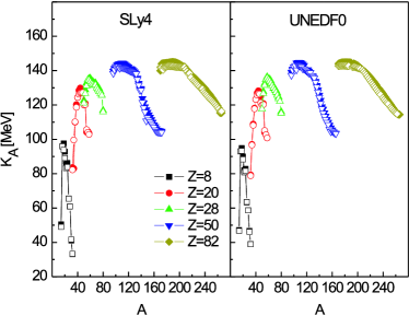
Figure 4: (Color online) Incompressibility $K_{A}$ calculated for the isotopic chains of semimagic nuclei with $Z=8$, 20, 28, 50, and 82. Left and right panels show results obtained for the SLy4 and UNEDF0 functionals, respectively. Full (empty) symbols correspond to the zero-range (separable) pairing force.

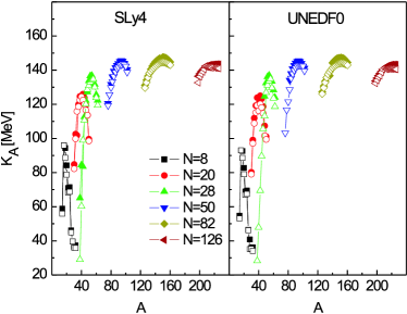
Figure 5: (Color online) Same as in Fig. 4, but for the isotonic chains with $N=8$, 20, 28, 50, 82, and 126.

To see effects of the pairing interaction in more detail, we focus on the results obtained for chains of tin and lead isotopes. In Figs. 6 and 7 we compare theoretical results with the experimental data for ²⁰⁸Pb and ^112-124Sn, taken from Refs. [You99] ; [Li07] ; [Li10] . A comparison of the two types of pairing interactions, and two different Skyrme functionals, leads to the conclusion that the calculated incompressibilities $K_{A}$ depend on the interactions in the particle-particle channel as well as the particle-hole channel of the two Skyrme functionals used in our study - SLy4 and UNEDF0 - only weakly. Of course, we can expect that using Skyrme parametrizations tuned to higher (lower) values of $K_{\infty}$ may lead to uniformly higher (lower) values of $K_{A}$.

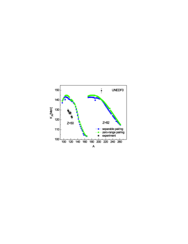
Figure 6: (Color online) Incompressibility $K_{A}$ calculated for chains of the $Z=50$ and 82 isotopes. Results obtained by using the separable (squares) and zero-range (circles) pairing with the UNEDF0 functional are compared to the available experimental data [You99] ; [Li07] ; [Li10] .

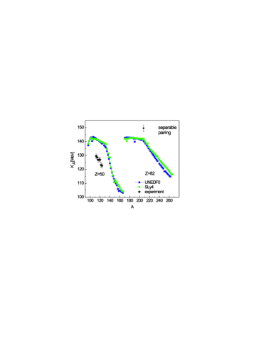
Figure 7: (Color online) Same as in Fig. 6, but for the UNEDF0 (squares) and SLy4 (circles) functionals and separable pairing force.

To check a weak dependence of $K_{A}$ on the intensity of pairing correlations, we have repeated the calculations by using values of neutron pairing strengths varied in a wide range, $G_{n}=631\pm 150$ MeV fm³ and $V_{n}=195\pm 30$ MeV fm³. Such variations induce very large changes of neutron pairing gaps, shown in Fig. 8; the ones that are certainly beyond any reasonable range of uncertainties related to adjustments of pairing strengths to data. In Figs. 9 and 10, we show the influence of the varied pairing strengths on the calculated incompressibilities $K_{A}$. We see clearly that even such large variations cannot induce changes compatible with discrepancies with experimental data.

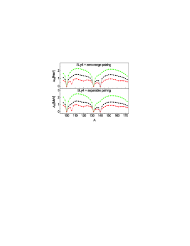
Figure 8: (Color online) Neutron pairing gaps calculated in tin isotopes for low (triangles), central (squares), and high (circles) values of pairing strength parameters given in captions of Figs. 9 and 10.

To illustrate the effect of isospin asymmetry, in Figs. 9 and 10 we plotted the results as functions of $N/Z$, whereby ¹²⁴Sn and ²⁰⁸Pb are located at almost the same point of the abscissa. These figures clearly show that the discrepancies with data are probably not related to the isospin dependence of $K_{A}$. Indeed, for both types of pairing, in the region of $1.0<N/Z<1.6$, the results obtained for tin and lead isotopes roughly follow each other.

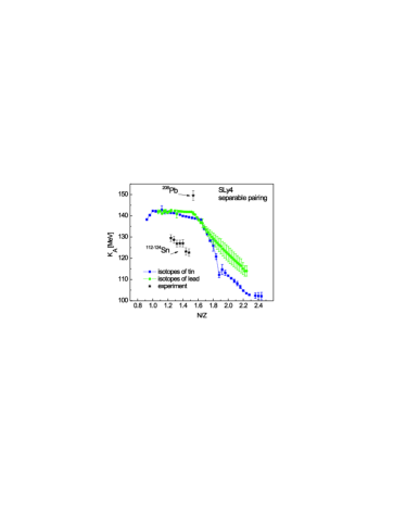
Figure 9: (Color online) Incompressibility $K_{A}$ calculated for the SLy4 functional and separable pairing force in tin (squares) and lead (circles) isotopes compared to the available experimental data. Theoretical results are plotted together with uncertainties pertaining to variations of the neutron strength parameter in the range of $G_{n}=631\pm 150$ MeV fm³.

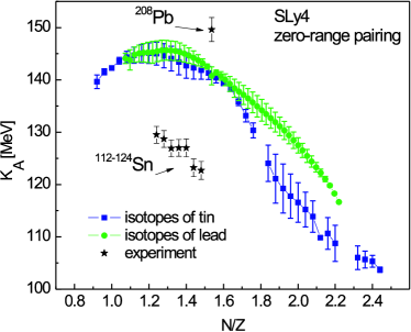
Figure 10: (Color online) Same as in Fig. 9, but for the zero-range pairing force and uncertainties pertaining to variations of the neutron strength parameter in the range of $V_{n}=195\pm 30$ MeV fm³.

Finally, to illustrate the fact that nuclear radii are fairly robust and cannot significantly influence the values of $K_{A}$, determined from Eqs. (30) and (31), we show values of $m_{1}/m_{0}$ alone in Figs. 11 and 12. We see that for both types of pairing, in tin and lead the calculated values of $m_{1}/m_{0}$ overestimate and underestimate the measured ones by 0.6–0.8 and 0.4 MeV, respectively. Exactly the same pattern was obtained within the relativistic nuclear energy density functionals studied in Ref. [Nik08a] , where the corresponding discrepancies were equal to 0.8–1.0 and 0.2 MeV. We also note that this comparison directly relates calculations to data, without using the intermediate and model-dependent definition of $K_{A}$.

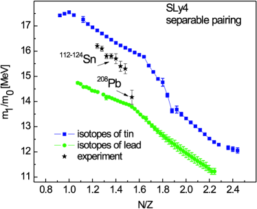
Figure 11: (Color online) Same as in Fig. 9, but for the centroids $m_{1}/m_{0}$.

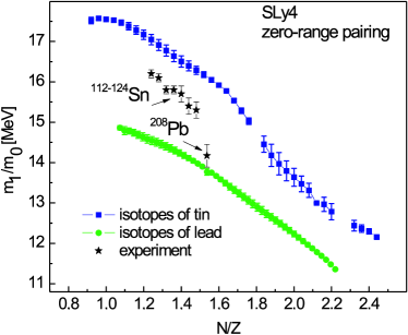
Figure 12: (Color online) Same as in Fig. 11, but for the zero-range pairing force.

To conclude our analysis, we have performed adjustments of the LD formula (32) to our microscopically calculated values of $K_{A}$. Since in the LD formula all parameters appear linearly, we could use the standard linear-regression method, which gave us the values of parameters that minimize $\chi^{2}$ along with standard estimates of statistical errors.

The obtained parameters are collected in Table 1. We see that the LD formula is able to provide an excellent description of the QRPA results, with average deviations of the order of 5 MeV, that is, about 3% of the typical value of $K_{A}$. Similarly the values of the volume incompressibility $K_{V}$ are determined to about 2% of precision. The least precisely determined LD parameter is the surface-symmetry incompressibility $K_{S,\tau}$, estimated up to 25% of precision. We also note that, within the fit precision, the volume parameter $K_{V}$ averaged over both functionals and both pairing forces equals to 254$\pm$5 MeV, which is significantly higher than the corresponding infinite-matter incompressibility of $K_{\infty}$=230 MeV. We would like to point out that the errors given in Table 1 are the statistical errors of the adjusted parameters and do not take into account possible systematic errors caused by using the model-dependent Eq. (30). Nevertheless, the results of the fit can be used as a useful parameterization of the microscopic calculations.

Table 1: Parameters (in MeV) of the LD formula (32) with standard errors, obtained by a fit to the values of $K_{A}$ calculated in $M$ semi-magic nuclei across the mass chart. The parameter $\chi$ was determined as the square root of the sum of fit residuals squared divided by the number of fit degrees of freedom ($M-5$ in our case).

	SLy4						UNEDF0
	separable			zero-range			separable			zero-range
$K_{V}$	252	$\pm$	5	258	$\pm$	5	249	$\pm$	5	257	$\pm$	4
$K_{S}$	$-$391	$\pm$	14	$-$406	$\pm$	13	$-$397	$\pm$	14	$-$412	$\pm$	13
$K_{\tau}$	$-$460	$\pm$	30	$-$500	$\pm$	30	$-$510	$\pm$	30	$-$550	$\pm$	30
$K_{S,\tau}$	410	$\pm$	110	560	$\pm$	100	570	$\pm$	120	740	$\pm$	100
$K_{C}$	$-$5.2	$\pm$	0.4	$-$5.4	$\pm$	0.4	$-$4.5	$\pm$	0.4	$-$5.1	$\pm$	0.4
$M$	210			211			204			195
$\chi$	5.0			4.7			5.3			4.4

VI Conclusions

In this work we have presented the first application of the separable, finite-range pairing interaction of the Gaussian form together with the non-relativistic functional of the Skyrme type. This interaction was used to determine both the ground-state Hartree-Fock-Bogolyubov solutions and Quasiparticle-Random-Phase-Approximation monopole strength functions in semi-magic nuclei. Results were systematically compared with those pertaining to the standard zero-range pairing interaction.

From the monopole strength functions, we extracted the finite-nucleus incompressibilities and compared them to experimental data. It turned out that neither zero-range nor separable pairing effects were able to describe the low values of incompressibilities measured in tin, relative to the high value measured in ²⁰⁸Pb. By changing the infinite-matter incompressibility, one can certainly describe either the tin or lead values; however, the high difference thereof remains unexplained.

The lack of agreement with experimental data is evident also in the case of the GMR centroids. This is even more important for the conclusions of our work, since the analysis of the centroids is not affected by the model-dependent extraction of incompressibilities by way of Eq. (30).

We have also performed adjustments of the LD formula to microscopically calculated incompressibilities, and we found that (i) such a formula is able to describe microscopic results very well, and (ii) the volume LD term is significantly higher than the infinite-matter incompressibility determined for a given functional.

VII acknowledgements

We thank Umesh Garg for discussions regarding the experimental data. This work was supported in part by the Academy of Finland and University of Jyväskylä within the FIDIPRO programme.

Appendix A Numerical tests

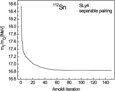
Figure 13: Convergence of the ratio of first and zero moments ${m_{1}}/{m_{0}}$ calculated in ¹¹²Sn as a function of the number of Arnoldi iterations.

Fig. 13 illustrates the reliability of the Arnoldi method in determining the key factors of our analysis, namely, the ratios of moments of the monopole strength functions. To obtain a perfectly stable result, only about 70 Arnoldi iterations suffice. In this way, the QRPA result is achieved within the CPU time that is of the same order as that needed to obtain a converged HFB ground state. Note that the Arnoldi iteration conserves all odd moments, so during the iteration, the moment ${m_{1}}$ does not change; thus the convergence of ${m_{1}}/{m_{0}}$ simply illustrates the convergence of ${m_{0}}$ alone.

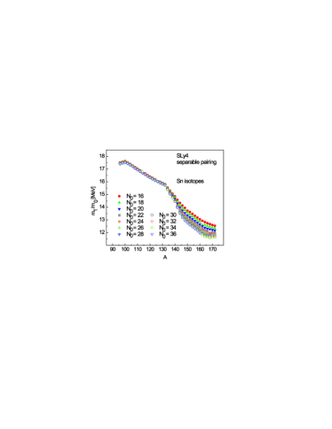
Figure 14: (Color online) Dependence of the ratio of first and zero moments ${m_{1}}/{m_{0}}$ on the number of HO shells $N_{0}$, calculated in tin isotopes.

The HO basis used in our calculations is characterized by two numerical parameters: frequency $\hbar\omega$ and number of shells included in the basis $N_{0}$. With varying particle numbers $A$, we use the standard prescription of

$$\hbar\omega=1.2\times 41\,\mbox{MeV}\times A^{-1/3},$$ (34)

established for the ground-state calculations [Dob97d] . Within this prescription, in Fig. 14 we study dependence of the QRPA moments ${m_{1}}/{m_{0}}$ on the number of HO shells $N_{0}$. One can see that in well-bound tin isotopes with $A\leq 132$, one obtains perfectly-well converged results. As is well known, in weakly-bound isotopes, owing to the effects of coupling to the continuum, the convergence properties gradually deteriorate and the HO-basis calculations become less reliable.

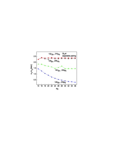
Figure 15: (Color online) Dependence of differences of ${m_{1}}/{m_{0}}$, calculated for pairs of tin and lead isotopes, on the number of HO shells $N_{0}$.

Nevertheless, as is often the case for restricted-space calculations, results pertaining to relative observables are much less basis-dependent. This is illustrated in Fig. 15, where we show differences of ratios of the QRPA moments ${m_{1}}/{m_{0}}$, calculated for pairs of tin and lead isotopes. We start form the pair of well-bound isotopes, ¹²⁴Sn and ²⁰⁸Pb, where experimental data are known, but we also show pairs with 8, 16, and 24 more neutrons. We see again that results for well-bound isotopes are perfectly-well converged. However, even for very exotic weakly-bound nuclei, the HO basis provides reasonably reliable results.

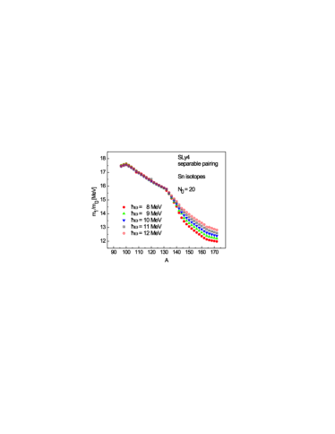
Figure 16: (Color online) Dependence of the ratio of first and zero moments ${m_{1}}/{m_{0}}$ on the HO frequency $\hbar\omega$, calculated in tin isotopes.

Finally, in Fig. 16 we show dependence of results on the HO frequency $\hbar\omega$, determined for $N_{0}=20$ HO shells. Note that the range of frequencies shown in the plot is much wider than those corresponding to prescription (34), which gives $\hbar\omega=10.60$ and 8.88 MeV for ¹⁰⁰Sn and ¹⁷⁰Sn, respectively. Nevertheless, no significant $\hbar\omega$-dependence is obtained for the $A\leq 132$ isotopes, whereas for weakly bound ones the estimated uncertainty does not exceed 1 MeV.

As an additional check, for the tin isotope ¹¹²Sn we performed the standard QRPA calculation by using the same $N_{0}=20$ configuration space as that used for our Arnoldi-method calculations. We found the spurious 0⁺ peak at a very small energy of $5.2\times 10^{-6}$ MeV, which guarantees a proper separation of the spurious mode from the physical spectrum.

References

- [1] J.P. Blaizot, Phys. Rep. 64, 171 (1980).
- [2] D.H. Youngblood, H.L. Clark, and Y.-W. Lui, Phys. Rev. Lett. 82, 691 (1999).
- [3] T. Li, U. Garg, Y. Liu, R. Marks, B.K. Nayak, P.V. Madhusudhana Rao, M. Fujiwara, H. Hashimoto, K. Kawase, K. Nakanishi, S. Okumura, M. Yosoi, M. Itoh, R. Matsuo, T. Terazono, M. Uchida, T. Kawabata, H. Akimune, Y. Iwao, T. Murakami, H. Sakaguchi, S. Terashima, Y. Yasuda, J. Zenihiro, and M.N. Harakeh, Phys. Rev. Lett. 99, 162503 (2007).
- [4] T. Li, U. Garg, Y. Liu, R. Marks, B.K. Nayak, P.V. Madhusudhana Rao, M. Fujiwara, H. Hashimoto, K. Nakanishi, S. Okumura, M. Yosoi, M. Ichikawa, M. Itoh, R. Matsuo, T. Terazono, M. Uchida, Y. Iwao, T. Kawabata, T. Murakami, H. Sakaguchi, S. Terashima, Y. Yasuda, J. Zenihiro, H. Akimune, K. Kawase, and M.N. Harakeh, Phys. Rev. C 81, 034309 (2010).
- [5] J. Piekarewicz, J. Phys. G: Nucl. Part. Phys. 37, 064038 (2010).
- [6] H. Sagawa, S. Yoshida, G.-M. Zeng, J.-Z. Gu, and X.-Z. Zhang, Phys. Rev. C 76, 034327 (2007).
- [7] J.M. Pearson, N. Chamel, and S. Goriely, Phys. Rev. C 82, 037301 (2010).
- [8] M. Centelles, S.K. Patra, X. Roca-Maza, B.K. Sharma, P.D. Stevenson, and X. Viñas, J. Phys. G: Nucl. Part. Phys. 37, 075107 (2010).
- [9] M.M. Sharma, Nucl. Phys. A 816, 65 (2009).
- [10] O. Civitarese, A.G. Dumrauf, M. Reboiro, P. Ring, and M.M. Sharma, Phys. Rev. C 43, 2622 (1991).
- [11] J. Li, G. Colò, and J. Meng, Phys. Rev. C 78, 064304 (2008).
- [12] T. Nikšić, D. Vretenar, and P. Ring, Phys. Rev. C 78, 034318 (2008).
- [13] V. Tselyaev, J. Speth, S. Krewald, E. Litvinova, S. Kamerdzhiev, N. Lyutorovich, A. Avdeenkov, and F. Grümmer, Phys. Rev. C 79, 034309 (2009).
- [14] E. Khan, Phys. Rev. C 80, 011307(R) (2009).
- [15] E. Khan, Phys. Rev. C 80, 057302 (2009).
- [16] E. Khan, J. Margueron, G. Colò, K. Hagino, and H. Sagawa, Phys. Rev. C 82, 024322 (2010).
- [17] J. Piekarewicz, Phys. Rev. C 76, 031301(R) (2007).
- [18] T. Duguet, Phys. Rev. C 69, 054317 (2004).
- [19] Y. Tian, Z. Y. Ma, and P. Ring, Phys. Lett. B 676, 44 (2009); Phys. Rev. C 79, 064301 (2009); Phys. Rev. C 80, 024313 (2009).
- [20] T. Nikšić, P. Ring, D. Vretenar, Y. Tian, and Z. Y. Ma, Phys. Rev. C 81, 054318 (2010).
- [21] B.G. Carlsson, J. Dobaczewski, and M. Kortelainen, Phys. Rev. C 78, 044326 (2008); 81, 029904(E) (2010).
- [22] J. Toivanen, B.G. Carlsson, J. Dobaczewski, K. Mizuyama, R.R. Rodríguez-Guzmán, P. Toivanen, and P. Veselý, Phys. Rev. C 81, 034312 (2010).
- [23] B.G. Carlsson, J. Dobaczewski, J. Toivanen, and P. Veselý, Comput. Phys. Commun. 181, 1641 (2010).
- [24] P. Ring and P. Schuck, The Nuclear Many-Body Problem (Springer-Verlag, Berlin, 1980).
- [25] J.P. Blaizot and G. Ripka, Quantum theory of finite systems, MIT Press, Cambridge Mass., 1986.
- [26] P. Avogadro and T. Nakatsukasa, Phys. Rev. C 84, 014314 (2011).
- [27] M. Baranger and K.T.R. Davies, Nucl. Phys. 79, 403 (1966).
- [28] S. Stringari, Phys. Lett. B108, 232 (1982).
- [29] S. Nishizaki and K. Ando, Prog. Theor. Phys. 73, 889 (1985).
- [30] E. Chabanat, P. Bonche, P. Haensel, J. Meyer, and R. Schaeffer, Nucl. Phys. A 635, 231 (1998).
- [31] M. Kortelainen, T. Lesinski, J. Moré, W. Nazarewicz, J. Sarich, N. Schunck, M.V. Stoitsov, and S. Wild, Phys. Rev. C 82, 024313 (2010).
- [32] J. Dobaczewski, W. Nazarewicz, T.R. Werner, J.-F. Berger, C.R. Chinn, and J. Dechargé, Phys. Rev. C 53, 2809 (1996).
- [33] B. Gall, P. Bonche, J. Dobaczewski, H. Flocard, and P.-H. Heenen, Z. Phys. A348, 183 (1994).
- [34] N. Schunck, J. Dobaczewski, J. McDonnell, W. Satuła, J.A. Sheikh, A. Staszczak, M. Stoitsov, P. Toivanen, Comp. Phys. Commun. 183, 166 (2012).
- [35] J. Dobaczewski and J. Dudek, Comput. Phys. Commun. 102, 183 (1997).