An equation-free approach
to coarse-graining the dynamics of networks

Abstract

We propose and illustrate an approach to coarse-graining the dynamics of evolving networks (networks whose connectivity changes dynamically). The approach is based on the equation-free framework: short bursts of detailed network evolution simulations are coupled with lifting and restriction operators that translate between actual network realizations and their (appropriately chosen) coarse observables. This framework is used here to accelerate temporal simulations (through coarse projective integration), and to implement coarse-grained fixed point algorithms (through matrix-free Newton-Krylov GMRES). The approach is illustrated through a simple network evolution example, for which analytical approximations to the coarse-grained dynamics can be independently obtained, so as to validate the computational results. The scope and applicability of the approach, as well as the issue of selection of good coarse observables are discussed.

I Introduction

Complex dynamic systems, exhibiting emergent dynamics, often arise in the form of graphs (or networks): the internet, social networks, chemical and biochemical reaction networks, communication networks and more Falo99power-law ; Albe02statistical ; Newm02random ; Newm03structure ; Aren06synchronizationa ; Bocc06complex ; Newm06structure ; Barr08dynamical ; Binz09topology ; Lain09dynamics ; Toiv09comparative . In a social network, for example, the individuals are represented by nodes (or vertices), while the relations among them are represented by the edges connecting these nodes.

One type of network dynamics arises in cases where the network topology (connectivity) is static, but the state of each vertex is a variable that evolves in time (in part due to interactions with the states of connected vertices). Such problems are said to exhibit “dynamics on networks”. A different type of network dynamics (on which we focus here) arises when the existence or the strength of connections between the vertices constitute the variables that evolve in time. These problems are said to exhibit “dynamics of networks”. These two types of dynamics are not, of course, mutually exclusive; clearly we can have dynamical problems involving dynamics both on and of networks. The evolutionary network problems we will refer to in this work will be exclusively of the second type of dynamics mentioned above: dynamics of networks, where the network structure is the state that changes over time. We will restrict ourselves to networks with unweighted edges, that are either present or absent; we will not study edges of continuously variable strength here, even though our methods can be adapted to function in such situations also (in fact, with appropriate modifications, in any type of network evolution problem).

In our networks of choice the detailed graph representation constantly changes over time according to some specified rules: edges (and/or nodes) are added or deleted. Although these fine-scale, “node level”, microscopic details of the graph are changing in time, coherence often emerges at a macroscopic level. At such a coarse-grained, system scale, the (expected) structure is often seen to evolve smoothly in time: it may eventually become stationary or may possibly oscillate between a number of states. We will use a coarse-grained, macroscopic view to study graph dynamics, treating the coarse temporal evolution as a dynamical system.

Reduced descriptions of high-dimensional dynamical systems (in our case, of large graphs) are possible predominantly due to two mechanisms: (a) decoupling of the evolution of a set of variables and/or (b) separation of time scales between evolution of different groups of variables. In the former (much simpler) case, the few uncoupled variables evolve independently of other variations in the system and hence a reduced closed description can be written in terms of just these variables. In the latter (more interesting) case, characteristic time scales of evolution of a few variables (called the “slow” variables) of the system are much longer than the time scales of evolution of the remaining “fast” variables. After a short evolution time the fast variables will then often become slaved to the slow variables, i.e., the evolution of the fast variables becomes (in the long term) solely determined by the evolution of the slow variables. The long-term dynamics of the system can therefore in principle be approximated by equations written only in terms of the slow variables, the “coarse variables” of the system. Note also that, depending on the time scales of interest, it may be possible to close the system (write closed form evolution equations) at different levels of detail.

To use the established tools and techniques of dynamical systems (e.g. bifurcation and stability computations), however, one must explicitly derive the evolution equations describing the coarse variable dynamics. We are interested in cases where such coarse evolution equations conceptually exist, yet they are not available in closed form. In such cases, it has been shown that it may be possible to circumvent their explicit derivation using equation-free techniques Kevr03equation-free ; Kevr04equation-free: . These techniques are based on short bursts of appropriately designed computational experiments with the detailed, “fine scale” network dynamic evolution model, and on the knowledge of the appropriate coarse observables: the variables in terms of which reduced closed coarse equations could in principle be written. Using traditional numerical algorithms as the basis for the design of computational experiments, and exploiting algorithms that translate between coarse variable values (relevant network statistics) and actual realizations of networks with these statistics, equation-free approaches may significantly accelerate the computer-assisted study of network dynamics. In recent work, we have applied equation-free techniques to illustrative examples of several different types: molecular dynamics Chen04from , collective animal behavior Moon07heterogeneous , cell population dynamics Bold07equation-free and also dynamical models on static networks Raje11coarse . Here, we demonstrate the use of equation-free techniques on an illustrative graph evolution problem, and test our results against explicitly derived coarse equations.

A crucial prerequisite for equation-free modeling is the knowledge of a good set of coarse variables - the collective network features that can be used to predict its (expected) coarse evolution, the variables in terms of which the coarse model would close. While a large graph is an intrinsically high dimensional object and difficult to visualize, its complicated structure can be probed by measuring statistical properties of the graph. Such statistical properties of graphs are often good candidate coarse variables. Commonly used statistical properties for describing a graph include the average degree, the degree distribution, the clustering coefficient, and the distributions of shortest path lengths. Newm03structure .

As we will see below, even after a good set of such coarse variables has been selected, an important requirement for using our equation-free algorithms is the ability to routinely construct graphs exhibiting prescribed values of these properties. It is clearly trivial to construct a graph with a given number of nodes and edges; yet it is quite non-trivial to construct realizations of graphs with, say, a prescribed distribution of shortest path lengths.

These issues will be discussed and illustrated through a simple model example in the remainder of the paper as follows: The model behavior is discussed briefly in Section II. We describe our coarse-graining approach in Section III. For our simple example, it so happens that several theoretical results can be explicitly obtained (and used for validation of the computer-assisted approach). These will be discussed in Sections IV and V. We will conclude with a brief summary and a discussion of the scope of the approach, its strengths and shortcomings, and of certain (in our opinion) important open research directions.

II Model: A random evolution of networks

We consider a simple, illustrative model of stochastic network evolution. Let the graph at any discrete time, $T=0,1,...$ be denoted by $G_{n}(T)$. The subscript $n$ denotes the number of nodes in the network. The rules governing the dynamics at each iteration can be described as follows:

1. Select a pair of nodes at random and connect them together by an edge if they are not already connected to each other.

2. With probability $r$, remove an edge chosen uniformly at random. ($r$ stands for removal probability.)

We performed numerical simulations using these detailed, node-level, “microscopic” rules (using $r=0.9$) on graphs with $n=100$ nodes and observed the evolution of several statistical graph properties over time. In these preliminary numerical experiments, the initial conditions were either empty graphs or Erdős-Rényi random graphs with a specified value of edge probability, $p$ (of which empty graphs are a special case, corresponding to $p=0$). It is interesting to consider the evolution of graph properties starting from an ensemble of initial conditions: Erdős-Rényi graphs with the same edge probability $p$. Fig.1 shows the evolution of one such property of interest: the degree distribution of the (nodes of the) graphs, obtained statistically from a $100$-copy sample. (The degree of a node in a network is the number of edges connected to the node.) The figure demonstrates that the degree distribution can be thought of as a function (ignoring, for the sake of simplicity, the discrete nature of the degree) that appears to evolve smoothly over time. Thus, the degree distribution can serve as a potential coarse observable of the system; one must, however, carefully investigate whether it is a good candidate for coarse variable.

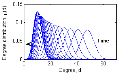
Figure 1: The (apparently) smooth evolution of degree distribution according to the model with $r=0.9$.

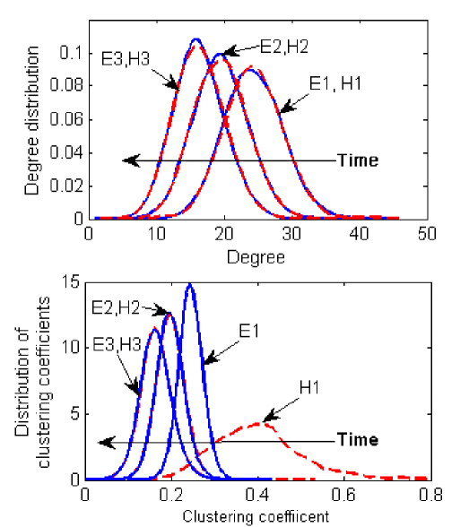
Figure 2: Evolution of (a) degree distribution and (b) triangle distribution, for two distinct ensembles of graphs. The solid (blue) curves represent the case where the initial graphs are chosen to be Erdős-Rényi graphs with $p=0.25$. The plots corresponding to this case are denoted by the labels, $E1$, $E2$ and $E3$ at times $0$, $10$ and $20$ respectively. Note that one time unit in the plot corresponds to $n=100$ iterations of the model. The dotted (red) curves represent the case where the initial graphs were created to match the degree distribution of the initial graphs of the previous Erdős-Rényi case through the Havel-Hakimi algorithm. The plots corresponding to this second case are denoted by the labels, $H1$, $H2$ and $H3$ at times $0$, $10$ and $20$ respectively.

In particular, one must test whether it is possible to obtain a description of the long-term evolution of this observable that is closed - that would imply that an accurate reduced model of the system evolution can, at least in principle, be derived. In other words, if one had measurements of the chosen set of coarse variables (observables) at particular time, that information alone should, in principle, be enough to predict future states of the system (in terms of these variables). We reiterate that, depending on the time scales of interest, different useful reduced models of the same system, i.e. closures at different levels of coarse description, may be possible to obtain.

We then proceeded to test whether the degree distribution constitutes a good choice of coarse observable. For this purpose we constructed initial graphs with identical degree distributions but different higher order information (triangle statistics, for instance), evolved the graphs using our model rules and compared their evolutions in time. Figures 2(a) and 2(b) show the evolution of degree distributions and of clustering coefficient distributions starting from graphs with identical degree distributions, but distinct distributions of clustering coefficients. (The clustering coefficient of a node is the ratio of the number of triangles attached to the node divided by the maximum possible number, given its degree.) The solid (blue) curves represent the case where the initial graph is an Erdős-Rényi graph ($p=0.25$). The dotted (red) curves corresponds to the case where the initial graphs were created to match the degree distribution of Erdős-Rényi graphs with $p=0.25$; this was done by sampling $n=100$ numbers (degrees) from the required degree distribution and using the Havel-Hakimi Have55remark algorithm to construct a graph with the sampled sequence of degrees. The Havel-Hakimi algorithm consists of three iterated steps:

1. sort the vertices by their degrees ($d_{i}$) in non-increasing order;

2. select the first vertex ($d_{1}$) and connect it to the next $d_{1}$ vertices; and

3. decrease the value of $d_{1}$ by $d_{1}$ (it is now 0) and the value of the $d_{1}$ successive degrees by 1.

As an illustration, consider the sorted list of residual degrees of the vertices (residual degree is the degree of a vertex minus the number of assigned edges for the same vertex at any given point in the algorithm)

$$d_{1}\geq d_{2}\geq...d_{n}.$$

Once we connect the first vertex with the next $d_{1}$ vertices, the residual degree sequence is

$$(0,d_{2}-1,d_{3}-1,...,d_{d_{1}+1}-1,d_{d_{1}+2},...).$$

After sorting, the sequence becomes

$$(d_{2}-1,d_{3}-1,...,d_{d_{1}+1}-1,...,0).$$

These steps are repeated until we get a sequence of zeros, implying that the graph with the desired degree sequence has been achieved.

For both our test cases, we thus have the same initial degree distribution. However, since the graphs themselves are different, properties like clustering coefficients will differ between them, at least initially. The model was evolved using $100$ copies to obtain smooth distribution functions. The figures show that the evolution of degree distribution is similar in both cases. Although the initial clustering coefficient distributions are very different for the two cases, they quickly (within a few time steps, compared to the time scale of evolution of the degree distribution) converge visually to the same function and subsequently coevolve. This suggests that the clustering coefficient distribution (and possibly other higher order information) may become quickly slaved to the evolution of the degree distribution: triangle statistics (and so also clustering coefficients) evolve at a much faster rate, and quickly reach a distribution that appears to depend only on the comparatively slowly evolving degree distribution. These results encourage us to attempt to find a coarse-grained reduction of the system using a discretization of the degree distribution as the coarse variable(s).

III Coarse-graining

We propose a computer-assisted coarse-graining approach –the Equation-Free (EF) framework Kevr03equation-free ; Kevr04equation-free: – to develop and implement a reduced description of the system, using the degree distribution as the coarse observable. In this approach, short bursts of simulations at the “microscopic” (individual node) level are used to estimate information (such as time-derivatives) pertaining to the coarse variables. This is accomplished by defining operators that allow us to translate between coarse observables and consistent detailed, fine realizations. The transformation from coarse to fine variables is called the lifting operator ($R$), while the reverse is called the restriction operator. If we denote the microscopic evolution operator by $\phi_{t}$, the macroscopic evolution operator can be defined as

$$\Phi_{t}(\cdot)=R\circ\phi_{t}\circ L(\cdot).$$

As an illustration, we implemented coarse projective integration Kevr03equation-free ; Kevr04equation-free: using the equation-free approach and the degree distribution as the coarse variable. In coarse projective integration, the system is integrated forward in time using occasional short bursts of detailed, microscopic simulations at the level of individual nodes, and the results are used to estimate time derivatives at the level of the degree distribution. In the following discussion, time units are taken to comprise $n=100$ iterations of the model. We used Erdős-Rényi random graphs ($p=0.25$) as the initial conditions and repeatedly performed the following operations:

1. Simulation: The model is executed initially for $10$ time steps (in each time step, we perform $n=100$ iterations of the rules of the model).

2. Restriction: The graph degree distributions, $\mu(d)$, are observed from simulations periodically (at intervals of $2$ time steps). We stored the degree distribution at discrete values $\mu_{i}=\mu(d_{i})$, where $d_{i}=0,1,2,...99$. The distribution may also be discretized using a smaller number of points and interpolated at intermediate values (we will discuss the possibility of alternative, more parsimonious representations below). In fact, our plots of degree distributions are smooth interpolations from this $100$ discrete value representation.

3. Projection forward in time: The time-series of the coarse variables over the final segment of the simulation (in our case, the last $3$ observed discretized degree distributions) are used to predict the new values of the coarse variables at a future time (in our case, $10$ time steps down the line). This is done on the basis of established numerical integration schemes (in our case, simple forward Euler). For the simple model differential equation $dx/dt=f(x)$, the forward Euler scheme would read

   $$x(t+\Delta t)\approx x(t)+\Delta tf^{\prime}(x(t)).$$

   The difference in our case is that the time derivative ($f^{\prime}(x(t))$ above) does not come form a closed formula, but is instead estimated from the recorded recent time series segments. In our computations, this time-derivative estimation and projection in time is performed as follows: Given the last $3$ observed discretized degree distributions, the associated $3$ cumulative distribution functions are found, and the degrees, $g_{i}$, corresponding to uniformly distributed percentile points, $p_{i}\in\{0,0.01,...1\}$, $i=1,....,101$, such that

   $$\int_{0}^{g_{i}}\mu(x)dx=p_{i}.$$

   Thus, the pairs of points $(g_{i},p_{i})$ constitute discrete approximations of the cumulative degree distributions. The values of these percentile degrees, $g_{i}$, observed at the last $3$ time steps, are the variables we actually projected forward in time, estimating the time derivative of the corresponding forward Euler scheme by fitting a straight line, and extrapolating it for $10$ further time steps. When projecting the discretized version of cumulative distributions, one should take care to retain monotonicity of the predicted (projected) distributionsmorefoot . In our simulations we did not encounter such a numerical problem, possibly because (a) we used several copies to get smoothened degree distributions, and (b) the projection times were relatively short.

4. Lifting: To restart the simulation, the predicted discretized distribution must be transformed into consistent graph realizations. We accomplish this by using the Havel-Hakimi algorithm; we may have to sample the projected degree distribution until we draw a graphical sequence of degrees. (A graphical sequence is a sequence on non-negative integers that is realizable as a degree sequence of a graph.) Checking if a sequence is graphical is performed as a part of the Havel-Hakimi algorithm: if the algorithm terminates successfully, the sequence is graphical; otherwise, it is not. In the latter case another sequence is sampled until a graphical one is found. Once we have these graphs, the procedure repeats: we continue simulations for $10$ more time steps as in stage $1$, keep the last $3$ observations, and so on.

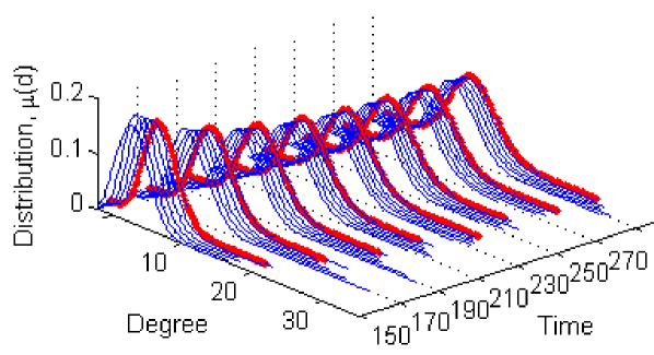
Figure 3: Coarse projective integration (CPI) with the degree distribution as the coarse variable. Results from CPI are plotted as (blue) thin lines every $2$ time steps during simulations, while results from direct simulation are plotted as (red) thick lines every $20$ time steps for comparison. Note that one time unit in the plot corresponds to $n=100$ iterations of the model.

The results of coarse-projective integration are shown as (blue) thin lines in Fig. 3 (note that degree distributions are plotted only when we collect simulation data, and not when we jump in time). The results from direct integration of the full model are plotted (red, thick lines) every $20$ time steps for comparison; the evolution of the degree distribution predicted by our coarse projective integration clearly coincides with the full detailed simulation.

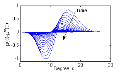
Figure 4: Decay of the degree distribution close to steady state: evolution of the difference between the instantaneous degree distribution $\mu(d)$ and the steady state degree distribution $\mu^{\infty}(d)$.

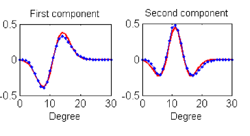
Figure 5: The first two PCA components of the ensemble of vectors $\mu(d)-\mu^{\infty}(d)$ shown in Fig. 4 are plotted as (blue) dotted lines. These components were found to be well-approximated by the analytical expressions $e^{(x-11)^{2}/20}(x-11)/5$ (first component, left) and $e^{(x-11)^{2}/20}(x-8)(x-14)/20$ (second component, right), plotted as (red) solid lines for reference.

We studied the rate of (temporal) convergence of discretized degree distribution as a given sample network evolution approaches steady (stationary) state. Fig. 4 shows the evolution of the difference between the instantaneous degree distribution $\mu(d)$ close to the steady state and the steady state degree distribution $\mu^{\infty}(d)$ itself. We used PCA to evaluate the first few principal components of the time sequence ($\mu(d)-\mu^{\infty}(d)$). The first two singular values were found to be $\approx 1.00$ and $0.0175$ respectively. The vectors corresponding to these first two singular values are plotted as (blue) dots in Fig. 5. These eigenvectors represent directions along which the decay of the degree distribution, from the given randomly chosen initial condition to the steady state, is the slowest. We found that the principal components were qualitatively similar for a wide variety of choices of initial graphs. For the specific example shown in the figure, the two principal components were found to be well-approximated by the analytical expressions $e^{(x-11)^{2}/20}(x-11)/5$ and $e^{(x-11)^{2}/20}(x-8)(x-14)/20$, which are plotted as (red) solid lines in the same figure. The relevance of the qualitative form of these principal components will be discussed later in Section V.

In addition to coarse projective integration, we also performed coarse fixed point computations. Instead of finding the (discretized) stationary degree distribution (coarse fixed point of the evolution) through direct simulation, one can also obtain it by solving the equation

$$F(\mu(d)):=\mu(d)-\Phi_{10}(\mu(d))=0,$$

where $\Phi_{t}$ is the coarse time-stepper over $t$ time steps. We find the roots of $F$ using a damped Newton-Krylov GMRES iteration scheme Saad86gmres: ; Kell95iterative . The standard Newton algorithm updates the value of $\mu(d)$ by $\mu_{n+1}(d)=\mu_{n}(d)+\Delta\mu(d)$, where $\Delta\mu(d)$ satisfying $[DF(\mu_{n}(d))]\Delta\mu(d)=-F(\mu_{n}(d)).$ Since $\Phi_{t}(\mu(d))$ is not explicitly available (but can be evaluated through the coarse time-stepper), its Jacobian cannot be obtained by analytical differentiation; in the Krylov-based approach the action of this Jacobian on known vectors (its matrix-vector products) are estimated through numerical directional derivatives. Thus, linear (and through them, nonlinear) equations are solved through iterative matrix-free computations; these methods are naturally suitable for equation-free computation, where explicit Jacobians are not available in closed form.

There are a couple of points worth mentioning about the use of this general methodology in the case where the unknowns solved for constitute a (discretized) distribution function $\mu(d)$: (a) the $\mu(d)$ vectors that arise should be non-negative and (b) they should integrate to $1$. At every iteration of the root-finding algorithm, these two properties should be preserved. These conditions on $\mu(d)$ can be stated as conditions on $\Delta\mu(d)$: $\Delta\mu(d)\leq-\mu_{n}(d)$ and $\Delta\mu(d)$ should integrate to $0$. We satisfy the first condition by using a damped Newton-Krylov method. The correction term $\Delta\mu(d)$ is scaled by a constant to ensure non-negativity of the result: $\mu_{n+1}(d)=\mu_{n}(d)+c\Delta\mu(d)$ for $c$ sufficiently small. The second condition is guaranteed by the structure of the Krylov method itself. When solving $[DF(\mu_{n}(d))]\Delta\mu(d)=-F(\mu_{n}(d))$ using a Krylov method, the solution $\Delta\mu(d)$ lies in the space spanned by $\{F(\mu_{n}(d)),[DF(\mu_{n}(d))]\cdot F(\mu_{n}(d)),...,[DF(\mu_{n}(d))]^{m}\cdot F(\mu_{n}(d))\}$ for some finite $m<n$. Because each of the spanning vectors has integral $0$, the update term $\Delta\mu(d)$ (and hence $c\Delta\mu(d)$, for any constant $c$) also has integral $0$. The convergence of this procedure can be shown by plotting $||\mu(d)-\phi(\mu(d))||$ at every iteration as in Fig. 6.

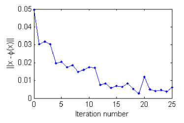
Figure 6: Convergence of the Newton-GMRES iterations in steady state computations: the norm of the function to be solved for via Newton-GMRES is plotted against the iteration number.

Coarse projective integration and coarse-fixed point algorithms are only two illustrations of equation-free computation: even though explicit coarse-grained evolution equations are not available, the assumption that they in principle exist helps solve the coarse-grained model through appropriately designed short bursts of detailed simulation (also through lifting and restriction). Many additional computational tasks (e.g. coarse continuation and bifurcation computations, coarse eigencomputations, coarse controller design and even optimization) also become possible in this framework Kevr09equation-free . Our computations so far provide numerical corroboration of the possibility of coarse-graining our network evolution model: a reduced model appears to close (accurately enough to be usefully predictive) in terms of only the (discretized) degree distribution. In what follows, we will provide certain theoretical results to support our choice of coarse variables and provide some intuition about the overall coarse-graining approach.

IV Theoretical justification

In this Section we discuss theoretical results that corroborate the observed separation of time scales between the evolution of our coarse variables (the discretized degree distribution) and higher order information about the evolving graph statistics (e.g. the distribution of triangles). Such information would support our ability to usefully close a coarse-grained model at the level of degree distributions.

For this simple graph evolution model, theoretical results for the evolution of edge density and vertex degrees can be easily derived using basic notions of probability; this was one of the reasons for choosing this model as our illustration. In general, for obtaining such results (including results for the evolution of triangles and more), one makes use of the notion of dense graph limits, which will be outlined later.

Recall that our model graphs evolve in discrete time steps according to the rules given in Section II. $G_{n}(T)$ denotes the graph in $n$ nodes at any discrete iteration, $T=0,1,...$ $G_{n}(T,i,j)$ is the entry in the corresponding adjacency matrix representing the edge between nodes $i$ and $j$. Let $E(G_{n}(T))$ represent the set of edges in the graph.

IV.1 Evolution of edge density

We denote by $e_{n}(T)=\left|{E(G_{n}(T))}\right|$ the number of edges in the graph at a given discrete time, $T$. Let $\bar{\rho}_{n}(T)$ be the edge density of the graph, $G_{n}(T)$ at time $T$:

$$\bar{\rho}_{n}(T):=\frac{e_{n}(T)}{\binom{n}{2}}.$$

Note that the evolution of $e_{n}(T)$ is itself a Markov chain, and that it is decoupled from the other variables:

$$\mathbf{P}\big{(}\,e_{n}(T\!+\!1)-e_{n}(T)=1\,\big{|}\,G_{n}(T)\,\big{)} =(1-\bar{\rho}_{n}(T))\cdot(1-r),$$ (1)

$$\mathbf{P}\big{(}\,e_{n}(T\!+\!1)-e_{n}(T)=0\,\big{|}\,G_{n}(T)\,\big{)} =(1-\bar{\rho}_{n}(T))\cdot r+\bar{\rho}_{n}(T)\cdot(1-r),$$ (2)

$$\mathbf{P}\big{(}\,e_{n}(T\!+\!1)-e_{n}(T)=-1\,\big{|}\,G_{n}(T)\,\big{)} =\bar{\rho}_{n}(T))\cdot r.$$ (3)

In order to study the evolution of $\bar{\rho}_{n}(T)$, we introduce the continuous time variable $t\in[0,\infty)$ and let $T=\lfloor\binom{n}{2}t\rfloor$, so that $T+1$ corresponds to $t+\mathrm{d}t$ with $\mathrm{d}t=\binom{n}{2}^{-1}$. Let $\rho_{n}(t):=\bar{\rho}_{n}(\lfloor\binom{n}{2}t\rfloor))$. It follows from (1), (2), (3) that we have

$$\mathbf{E}\big{(}\,\rho_{n}(t+\mathrm{d}t)-\rho_{n}(t)\,\big{|}\,\rho_{n}(t)\,\big{)} =(1-r-\rho_{n}(t))\mathrm{d}t,$$ (4)

$$\mathbf{D}^{2}\left(\rho_{n}(t+\mathrm{d}t)-\rho_{n}(t)\,\big{|}\,\rho_{n}(t)\right) =\big{(}(1-\rho_{n}(t))\rho_{n}(t)+r\cdot(1-r)\big{)}\binom{n}{2}^{-1}\mathrm{d}t.$$ (5)

Letting our process evolve for $T\asymp n^{2}$ steps (i.e. $t\asymp 1$), we obtain

$$\mathbf{E}\big{(}\,\rho_{n}(t)-\rho_{n}(0)\,\big{)} \stackrel{{\scriptstyle\eqref{edgedens_condexpect}}}{{\asymp}}T\cdot\mathrm{d}t\asymp 1,$$

$$\mathbf{D}^{2}\left(\rho_{n}(t)-\rho_{n}(0)\right) \stackrel{{\scriptstyle\eqref{edgedens_condvar}}}{{\asymp}}T\cdot\binom{n}{2}^{-1}\mathrm{d}t\asymp n^{-2}.$$

Since the variance of $\rho_{n}(t)-\rho_{n}(0)$ in the above formulas is much smaller than its expected value if $1\ll n$, we can replace $\rho_{n}(t)$ by $\mathbf{E}(\rho_{n}(t))$ in (4) without causing significant error. This leads to the deterministic equation

$$\frac{\mathrm{d}}{\mathrm{d}t}\rho(t)=(1-r)-\rho(t)$$ (6)

for $\rho(t)$, the limit $\rho_{n}(t)\to\rho(t)$ as $n\to\infty$, corresponding to (4). Thus

$$\rho(t)=(1-r)+(\rho(0)-(1-r))e^{-t}$$ (7)

and $\lim_{t\to\infty}\rho(t)=1-r$.

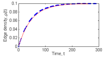
Figure 7: Coarse projective integration (CPI) of the edge density evolution: Results obtained from CPI using edge density as the coarse variable are plotted as blue dots (see text for details). The trajectory obtained from full direct simulation (red solid line) is plotted for reference. One time unit in this plot corresponds to $n=100$ iterations of the model.

From (6), it is clear that the evolution of edge density $\rho(t)$ is truly decoupled from the evolution of other quantities - one does not need the higher order statistics of the graph to get slaved to it over a short time period on a sort of slow manifold for the reduced model to close. As mentioned earlier, this represents one type of conditions for which reduced descriptions of the system become possible. In Section III we computationally implemented a reduced model using the entire degree distribution as the coarse observable(s). (6) represents an even more reduced description that meaningfully closes in terms of edge density. Similar to the degree distribution case, we implement coarse-projective integration using now only edge density as the coarse variable. The single scalar value of the edge density was observed and recorded during brief bursts of direct simulation; the time horizons for direct simulation and subsequent projection forward in time were again chosen to be $10$ time steps each. The lifting operation in this case involves creating graphs with a given value of edge density. Our particular implementation of this created graphs where every edge was selected to be present with a probability equal to the edge density. The results of coarse projective integration with the empty graph as initial condition, shown as (blue) dots in Fig. 7, agrees visually with the evolution of edge density as observed from direct simulations, shown as a (red) solid line. This corroborates the closure of a reduced description in terms of edge density only. We now proceed to derive results supporting our previous observation of closure of a reduced description at the more detailed (less coarse) level of degree distribution.

IV.2 Evolution of the degree of a vertex

Consider the time evolution of the degree of a node $i\in[n]$, i.e. the number of other vertices $i$ is connected to. The order of magnitude of the degree of $i$ is $n$. Define a normed degree, $D_{n}(t)$, of a vertex $i$ at scaled time $t$ as

$$D_{n}(t):=\frac{1}{n}\sum_{j=1}^{n}G_{n}(\lfloor t\binom{n}{2}\rfloor,i,j);$$ (8)

we omit the $i$-dependence from the $D_{n}(t)$ notation for the sake of simplicity. Following a derivation similar to the one used in Section IV.1, we obtain:

$$\mathbf{E}\big{(}\,D_{n}(t+\mathrm{d}t)-D_{n}(t)\,\big{|}\,G_{n}(t)\,\big{)} =\left(1-\left(1+\frac{r}{\rho_{n}(t)}\right)D_{n}(t)\right)\mathrm{d}t,$$ (9)

$$\mathbf{D}^{2}\left(D_{n}(t+\mathrm{d}t)-D_{n}(t)\,\big{|}\,G_{n}(t)\right) =\left(1-D_{n}(t)+r\frac{D_{n}(t)}{\rho_{n}(t)}\right)n^{-1}\mathrm{d}t.$$ (10)

Now (10) is of smaller order than (9) if $n\gg 1$, so that we may replace $D_{n}(t)$ by $\mathbf{E}(D_{n}(t))$. By analogy with the argument of subsection IV.1 we see that $D_{n}(t)\to D(t)$ as $n\to\infty$, where $D(t)$ solves the ODE

$$\frac{\mathrm{d}}{\mathrm{d}t}D(t)=1-\left(1+\frac{r}{\rho(t)}\right)D(t).$$ (11)

Substituting the explicit formula (7) into (11) and using the formula for the solution of inhomogenous linear ODEs, we obtain an explicit solution for $D(t)$:

$$D(t)=\rho(t)+{e}^{\frac{-t}{1-r}}{\rho(t)}^{\frac{-r}{1-r}}\left(\rho(0)^{\frac{r}{1-r}}D(0)-\rho(0)^{\frac{1}{1-r}}\right).$$ (12)

Clearly, $\lim_{t\to\infty}D(t)=\lim_{t\to\infty}\rho(t)=1-r$.

Note that the evolution of the degree of a given vertex depends both on its current degree and the current edge density of the graph as a whole. Yet, if the degree distribution of a graph is given, the edge density of the graph also follows from it. This clearly supports our observation that the system closes at the level described in Section III: in terms of the degree distribution. Approximate differential equations were derived so far to describe the evolution of (expected values of) the normed degree and of the edge density of graphs. The next step is to explore the dynamics and influence of higher order information, like triangles. In order to derive similar results for statistics of triangles, we take advantage of concepts from the theory of convergent dense graph sequences, of which a rigorous and formal introduction can be found in Lov06limits .

IV.3 Convergent dense graph sequences

Let $G_{n}(T)$ denote the adjacency matrices of our evolving graphs, and let the individual entry representing the existence of an edge between nodes $i\in[n]$ and $j\in[n]$ at time $T$ be denoted by $G_{n}(T,i,j)$. The notion of dense graph limits will be useful for describing the time evolution of the statistical properties of $G_{n}(T)$ when $n\gg 1$. The limit object of a convergent graph sequence is a so-called graphon $W$, where $W:[0,1]^{2}\to[0,1]$ is a measurable (but not necessarily continuous) function with the properties $W(x,y)=W(y,x)$ and $W(x,x)=0$. Assume that for each $n\in\mathbb{N}$ we have a graph $G_{n}$ with vertex set $[n]$. We now informally define the notion of convergence of the sequence $G_{n}$ to $W$, i.e. $G_{n}\to W$.

One might heuristically imagine the adjacency matrix of $G_{n}$ as a black-and-white television screen (a white pixel at position $(i,j)$ represents an edge between vertices $i$ and $j$); a convergent graph sequence becomes then a sequence of TV sets showing the same picture at higher and higher resolution. The limiting graphon $W$ will then be the picture seen on the “perfect TV” where each point $(x,y)\in[0,1]^{2}$ is a “pixel of infinitesimal size”; the local density of black/white pixels will then give us the impression of shades of grey. For the precise definition of the so-called cut-distance $\delta(G_{n},W)$ between a finite graph and a graphon, see (Lov09very, ; Lov09very1, , Section 4). Note that by (Lov09very, , Theorem 6.13) every graphon $W$ arises as a limit for a convergent graph sequence $G_{n}$.

Clearly, there exist many adjacency matrices corresponding to different labelings of the nodes of the same graph, and in the definition of $G_{n}\to W$ we are allowed to relabel the vertices of $G_{n}$ (i.e. to rearrange the pixels our TV set). Correspondingly, we are allowed to relabel $[0,1]$ using measure-preserving transformations in order to obtain equivalent forms of the graphon $W$ (see (Lov09very, , Section 3.1)). For the purposes of the present paper, accounting for rearrangements is not required.

If $F$ is the adjacency matrix of a small graph on $k$ nodes, then we define the homomorphism density $t(F,G_{n})$ by

$$t(F,G_{n}):=\frac{1}{{n\choose k}k!}\!\sum_{\varphi:[k]\to[n]}\!1{\hskip-2.5pt}\hbox{I}\left[\forall i,j\in[k]\!:\!F(i,j)\!\leq\!G_{n}(\varphi(i),\varphi(j))\right],$$ (13)

where we sum over all possible injective functions $\varphi$ from $[k]$ to $[n]$. $F$ is our test graph and $t(F,G_{n})$ the homomorphism density of $F$ in $G_{n}$.

We define the homomorphism density of $F$ in $W$ by

$$t(F,W)=\int_{0}^{1}\!\dots\!\int_{0}^{1}\!\prod_{1\leq i<j\leq k}\!W(x_{i},x_{j})^{F(i,j)}\mathrm{d}x_{1}\dots\mathrm{d}x_{n}.$$ (14)

Denote by $K_{k}$ the complete graph on $k$ vertices; for example, $K_{2}$ is an edge and $K_{3}$ is a triangle. Erasing an edge from a triangle gives a “cherry”, a simple graph with three vertices and two edges.

Now, denote by $\rho_{n}:=\frac{\left|{E(G_{n})}\right|}{\binom{n}{2}}$ the edge density of $G_{n}$. It follows from (Lov09very, , Section 6.2) that $G_{n}\to W$ implies $t(F,G_{n})\to t(F,W)$:

$$\rho_{W}:=\lim_{n\to\infty}\rho_{n}=\lim_{n\to\infty}t(K_{2},G_{n})=t(K_{2},W)=\int_{0}^{1}\int_{0}^{1}W(x,y)\mathrm{d}x\mathrm{d}y,$$ (15)

$$\lim_{n\to\infty}t(K_{3},H_{n})=t(K_{3},W)=\int_{0}^{1}\int_{0}^{1}\int_{0}^{1}W(x,y)W(y,z)W(z,x)\mathrm{d}x\mathrm{d}y\mathrm{d}z,$$ (16)

$$\lim_{n\to\infty}t(\text{cherry},H_{n})=t(\text{cherry},W)=\int_{0}^{1}\int_{0}^{1}\int_{0}^{1}W(x,y)W(y,z)\mathrm{d}x\mathrm{d}y\mathrm{d}z.$$ (17)

It is the ability to write such equations that makes working with graphons useful for our purposes. Once the graphon is identified, one can approximate the density of any test graph $F$ in $G_{n}$, $1\ll n$ using expressions similar to Equations (15), (16), (17).

IV.4 Evolution of the graphon

If we consider a convergent graph sequence $H_{n}\to W$, where $H_{n}$ is a graph on $n$ vertices, and for each $n$ we run our Markov process $G_{n}(T)$ with initial state $G_{n}(0)=H_{n}$, then

$$G_{n}(\lfloor\binom{n}{2}t\rfloor)\to W_{t},$$

where $W_{t}(x,y)$ is the solution of the following ODE:

$$\frac{\mathrm{d}}{\mathrm{d}t}W_{t}(x,y)=1-\left(1+\frac{r}{\rho(t)}\right)W_{t}(x,y).$$ (18)

The heuristic derivation (20) of this formula is based on

$$W_{t}(x,y)\approx\mathbf{P}\big{(}\,G_{n}(\lfloor\binom{n}{2}t\rfloor,\lfloor x\cdot n\rfloor,\lfloor y\cdot n\rfloor)=1\,\big{)}$$ (19)

where $T=\lfloor\binom{n}{2}t\rfloor$, $\mathrm{d}t=\binom{n}{2}^{-1}$, $i=\lfloor x\cdot n\rfloor$, $j=\lfloor y\cdot n\rfloor$. Note that $e(T)\approx\rho(t)\binom{n}{2}$.

$$W_{t+\mathrm{d}t}(x,y)-W_{t}(x,y)=\\ \mathbf{P}\big{(}\,G(T+1,i,j)=1\,\big{|}\,G(T,i,j)=0\,\big{)}\cdot(1-W_{t}(x,y))-\\ \mathbf{P}\big{(}\,G(T+1,i,j)=0\,\big{|}\,G(T,i,j)=1\,\big{)}\cdot W_{t}(x,y)=\\ \binom{n}{2}^{-1}\cdot(1-W_{t}(x,y))-\frac{r}{e(T)}\cdot W_{t}(x,y)=\\ \Big{(}1-\left(1+\frac{r}{\rho(t)}\right)W_{t}(x,y)\Big{)}\mathrm{d}t.$$ (20)

This results in (18).

By substituting the explicit formula (7) into (18) and using the integral formula for the solution of inhomogenous linear ODEs, we obtain an explicit solution for $W_{t}(x,y)$:

$$W_{t}(x,y)=\rho(t)+{e}^{\frac{-t}{1-r}}{\rho(t)}^{\frac{-r}{1-r}}\left(\rho(0)^{\frac{r}{1-r}}W_{0}(x,y)-\rho(0)^{\frac{1}{1-r}}\right).$$ (21)

We have $\lim_{t\to\infty}W_{t}(x,y)=\lim_{t\to\infty}\rho(t)=1-r$. Thus for $t\gg 1$ the graphon becomes almost constant with value $1-r$; (19) shows that the stationary state of our graph dynamics looks like an Erdős-Rényi graph with edge density $1-r$. In addition, (18) implies that an initially constant graphon will remain constant at future times. Thus, the family of Erdős-Rényi graphs is an invariant set of the dynamics of system.

Note that, given the explicit formula for $W_{t}(x,y)$ we may obtain an explicit formula for the density of triangles and cherries in $G_{n}(T)$ using (16) and (17). Differential equations for describing the evolution of triangles and cherry densities at time $t$ can be found directly by differentiating those equations.

IV.5 Evolution of cherry and triangle densities

Recalling (17) we have

$$t(\text{cherry},W_{t})=\int_{0}^{1}\int_{0}^{1}\int_{0}^{1}W_{t}(x,y)W_{t}(y,z)\mathrm{d}x\mathrm{d}y\mathrm{d}z.$$

Differentiating (17) with respect to time and using the graphon evolution result of (18), we get

$$\frac{\mathrm{d}}{\mathrm{d}t}t(\text{cherry},W_{t})=2\!\int_{0}^{1}\!\int_{0}^{1}\!\int_{0}^{1}\!\left(1-\left(\!1+\frac{r}{\rho(t)}\!\right)\!\!\!W_{t}(x,y)\right)W_{t}(y,z)\mathrm{d}x\mathrm{d}y\mathrm{d}z=\\ 2\rho(t)-2\left(1+\frac{r}{\rho(t)}\right)t(\text{cherry},W_{t}).$$ (22)

An ODE describing the time evolution of the density of triangles (in terms of the edge density and the cherry density) can be similarly derived:

$$\frac{\mathrm{d}}{\mathrm{d}t}t(K_{3},W_{t})=3~{}t(\text{cherry},W_{t})-3\left(\!1+\!\frac{r}{\rho(t)}\!\right)t(K_{3},W_{t}).$$ (23)

IV.6 Convergence rates

Now that we have equations describing the statistics of degrees, cherries and triangles, we can find out the rates at which these quantities converge to their steady (stationary) states. A function $a(t)$ converges to another function $b(t)$ at rate $\alpha$ if

$$\lim_{t\to\infty}\frac{1}{t}\log(\left|{a(t)-b(t)}\right|)=-\alpha.$$

In order to establish this, it is enough to prove that

$$\lim_{t\to\infty}\frac{1}{\left|{a(t)-b(t)}\right|}\frac{\mathrm{d}}{\mathrm{d}t}\left|{a(t)-b(t)}\right|=-\alpha.$$

From (7) we can directly see that the edge densities of our graphs converge to the steady state value of $1-r$ at a rate $\alpha=1$. This can also be shown by using (6) to write the following equation:

$$\frac{\mathrm{d}}{\mathrm{d}t}\left(\rho(t)-(1-r)\right)\;=\;-\left(\rho(t)-(1-r)\right).$$

We now show that the normed degree $D(t)$ of a vertex converges to $\rho(t)$ at a faster rate. From (6),(11) we obtain

$$\frac{\mathrm{d}}{\mathrm{d}t}\left(D(t)-\rho(t)\right)=-\left(1+\frac{r}{\rho(t)}\right)\left(D(t)-\rho(t)\right).$$ (24)

Thus $\alpha=\lim_{t\to\infty}\left(1+\frac{r}{\rho(t)}\right)=\frac{1}{1-r}$ in this case. Note that $\alpha=\frac{1}{1-r}$ also follows from the explicit formula (12). For example, if $r=0.9$ then $\alpha=10.$

From (18), we similarly obtain that for any $x,y\in[0,1]$ the function $W_{t}(x,y)$ converges to $\rho(t)$ at a rate $\alpha=\frac{1}{1-r}$.

If the graphon $W_{t}$ evolves according to (18) and $\rho(t)=\int_{0}^{1}\int_{0}^{1}W_{t}(x,y)\mathrm{d}x\mathrm{d}y$ then $\rho(t)$ solves (6). If we let $\hat{W}_{t}(x,y)=\rho(t)$ for any $x,y\in[0,1]$ then $\hat{W}_{t}$ also solves (18). Thus, the set of constant graphons is invariant under the dynamics. We now show evidence that this “invariant manifold” is actually attracting:

$$\frac{\mathrm{d}}{\mathrm{d}t}\left(t(\text{cherry},W_{t})-t(\text{cherry},\hat{W}_{t})\right)\stackrel{{\scriptstyle\eqref{cherrydens_111}}}{{=}}\frac{\mathrm{d}}{\mathrm{d}t}\left(t(\text{cherry},W_{t})-\rho(t)^{2}\right)\stackrel{{\scriptstyle\eqref{cherry_density_ode},\eqref{ode_edge_density1}}}{{=}}\\ 2\rho(t)-2\left(1+\frac{r}{\rho(t)}\right)t(\text{cherry},W_{t})-2\rho(t)(1-r-\rho(t))=\\ -2\left(1+\frac{r}{\rho(t)}\right)\left(t(\text{cherry},W_{t})-t(\text{cherry},\hat{W}_{t})\right).$$ (25)

This implies that $t(\text{cherry},W_{t})$ converges to $t(\text{cherry},\hat{W}_{t})$ at rate $\alpha=2\frac{1}{1-r}$. If $r=0.9$ then $\alpha=20$ for this case. Thus, if we evolve graphs that already possess the steady state values of their edge density, their cherries will converge to their steady state value twice as fast as the rate at which normed degrees evolve to their corresponding steady state.

We now consider triangle density evolution. Let $W^{1}$ and $W^{2}$ be two distinct graphons with the same values of edge and cherry densities:

$$t(K_{2},W^{1}\!)\!=\!t(K_{2},W^{2}\!)\text{ and }t(\text{cherry},W^{1}\!)\!=\!t(\text{cherry},W^{2}\!)$$

If we let $W^{1}_{t}$ and $W^{2}_{t}$ evolve according to the dynamics (18) with initial states $W^{1}$ and $W^{2}$, respectively, then by (6) and (22) we have

$$t(K_{2},W_{t}^{1}\!)\!=t(K_{2},W_{t}^{2}\!),\;t(\text{cherry},W_{t}^{1}\!)\!=\!t(\text{cherry},W_{t}^{2}\!)$$ (26)

for all $t\geq 0$. The fact that the density of edges and cherries coincide for $W^{1}_{t}$ and $W^{2}_{t}$ “helps” the densities of triangles in $W^{1}_{t}$ and $W^{2}_{t}$ to converge to each other even more rapidly:

$$\frac{\mathrm{d}}{\mathrm{d}t}\left(t(K_{3},W^{1}_{t})-t(K_{3},W^{2}_{t})\right)\stackrel{{\scriptstyle\eqref{triangle_density_ode}}}{{=}}-3\left(1+\frac{r}{\rho(t)}\right)\left(t(K_{3},W^{1}_{t})-t(K_{3},W^{2}_{t})\right).$$ (27)

Thus the rate of convergence of the relative triangle density is $\alpha=3\frac{1}{1-r}$: for $r=0.9$ this works out to be $30$. This result, in particular, explains why we observed an apparent slaving of the triangles, as discussed in in Fig. 2. The (blue) solid and (red) dotted curves there showed the evolution of two graphs with the same degree distribution. Graphs with the same degree sequence also have the same number of edges and cherries, which implies (26). The number of triangles in these two graphs (corresponding to the two cases in Fig.2) converge to each other three times as fast as the rate at which the degree distributions ultimately evolve.

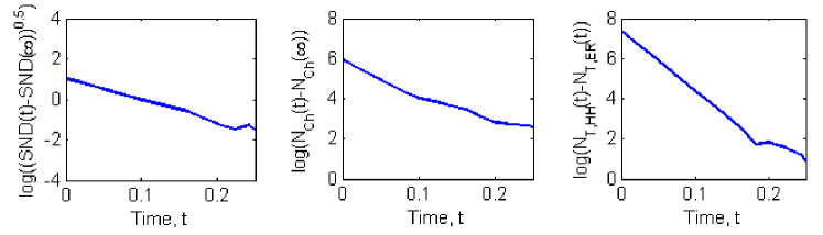
Figure 8: Evolution of the logarithms of quantities related to (a) degree, (b) cherries and (c) triangles. The initial conditions for the three cases are explained in the text. SND denotes the sum of squares of the normed sequence of degrees of all the $100$ nodes. $N_{Ch}$ denotes the number of cherries in the graph. $N_{T,ER}$ and $N_{T,HH}$ denote the number of triangles in two graph evolutions starting with an Erdős-Rényi random graph with $p=0.1$ and a graph created using the Havel-Hakimi algorithm respectively, both with the same degree distribution. Note that one time unit in this plot corresponds to $\binom{n}{2}=4950$ iterations of the model. Slopes of the three lines are $-10.44$, $-18.49$ and $-29.98$ respectively, which are in close agreement with theoretical results of $-10$, $-20$ and $-30$ respectively.

We now estimate convergence rates from direct simulation results, confirming the validity of our approach and approximations even for relatively small systems: in these results $n=100$ nodes and we simulate the model using a value of $0.9$ for the parameter $r$. Figure 8 shows how information about degrees, cherries and triangles converge to their corresponding steady (stationary) states. Note that, in all these cases, the time $t$ is scaled so that one time unit comprises $\binom{n}{2}$ iterations of the model. Logarithms of quantities (defined in the caption of the figure) related to these statistics are plotted in the y-axis versus time. For producing the first two plots (corresponding to degrees and cherries), the initial graphs were created by first sampling from a normal degree distribution with mean $10$ and standard deviation of $1$. For comparison, the steady state graphs have a degree distribution whose mean and standard deviation were evaluated to be $\approx 10$ and $\approx 3$ respectively. Thus, the initial graphs have the same mean degree (and hence the same edge density) as the steady state graphs, but differ from these steady state graphs in their actual detailed degree distribution. Since the graphs are initialized with the steady state edge density, this edge density remains close to its steady state value at all times. From (24) and (25), the convergence rates for the quantities in the first two figures are expected to be $10$ and $20$ respectively. This successfully matches the numerical convergence rates (the absolute values of the slopes of evolutions) of the terms related to degrees and cherries in the figure: they are seen to be $10.44$ and $18.49$ respectively. For the third plot, containing information about triangles, we simulate the model from two different initial graphs with the same degree distribution but different number of triangles. The first simulation is initialized with an Erdős-Rényi random graph with $p=0.1$. For the second case, we created initial graphs using the Havel-Hakimi algorithm, using the degree sequence of the first case as input. Since graphs with the same degree sequence also have the same number of edges and cherries, (26) is satisfied. Hence from (27), we expect a convergence rate of $30$ for the relative number of triangles between these two graphs, which successfully matches the numerically computed value of $29.98$. Thus, although the theoretical results are in principle accurate only at the limit of very large graphs, all the numerical values we computed using graphs with only $100$ nodes are remarkably close to the limiting theoretical values.

V Some additional theoretical results

V.1 An SDE for the degree of a vertex

In the previous section we approximated the evolution of the normed degree through a deterministic ODE, arguing for the relative smallness of the order of magnitude of the variance of what is really a stochastic process. In order to now describe the evolution of the stochastic process $D_{n}(t)$ at a finer level, we approximate it by a stochastic differential equation (SDE) rather than an ODE:

$$\mathrm{d}D_{n}(t)=\left(1-D_{n}(t)-r\frac{D_{n}(t)}{\rho_{n}(t)}\right)\mathrm{d}t+\sqrt{1-D_{n}(t)+r\frac{D_{n}(t)}{\rho_{n}(t)}}\cdot n^{-1/2}\mathrm{d}W_{t},$$ (28)

where $W_{t}$ now denotes the standard Brownian motion. To rationalize the choice of such an approximation, we observe that the solution of (28) satisfies (9) and (10) and that the $D_{n}(t)$ defined by (8) satisfies $|D_{n}(t+\mathrm{d}t)-D_{n}(t)|\leq\frac{1}{n}$, i.e. the trajectory of $D_{n}(t)$ is very close to being continuous. One can then suggest that it is appropriate (and even natural) to use the Brownian motion in (28) as a driving function. For rigorous results validating the SDE approximation of discrete stochastic processes, see Ispa10note .

We are interested in the fluctuations of $D_{n}(t)$ around its expected value $\tilde{D}_{n}(t)=\mathbf{E}\big{(}\,D(t)\,\big{)}$. Using (9) we can see that $\tilde{D}_{n}(t)$ approximately solves the ODE

$$\mathrm{d}\tilde{D}_{n}(t)=\left(1-\tilde{D}_{n}(t)-r\frac{\tilde{D}_{n}(t)}{\rho_{n}(t)}\right)\mathrm{d}t.$$ (29)

If we define $X(t):=n^{1/2}(D(t)-\tilde{D}_{n}(t))$ then by (28) and (29) $X(t)$ solves the SDE

$$\mathrm{d}X(t)=-\left(1+\frac{r}{\rho_{n}(t)}\right)X(t)\mathrm{d}t+\sqrt{1-D_{n}(t)+r\frac{D_{n}(t)}{\rho_{n}(t)}}\mathrm{d}W_{t}.$$ (30)

If $n$ is big enough, then ${\rho}_{n}(t)\approx\rho(t)$ and $D_{n}(t)\approx\tilde{D}_{n}(t)\approx D(t)$, so we may use the deterministic $\rho(t)$ and $D(t)$ in the right-hand side SDE of $X(t)$ without causing much error.

Since $\rho(t)$ and $D(t)$ are known and explicit (c.f. (7), (12)), (30) is a linear SDE, i.e. an Ornstein-Uhlenbeck process with time-dependent drift and diffusion coefficient. From this, it follows that $X(t)$ can be approximated by a Gaussian process with mean $0$ and an explicit formula for the variance at time $t$. If we let $t\to\infty$ then $\rho(t)\to 1-r$ and $D(t)\to 1-r$, so (30) becomes

$$\mathrm{d}X(t)=-\frac{1}{1-r}X(t)\mathrm{d}t+\sqrt{2r}\mathrm{d}W_{t},$$ (31)

an OU process. The variance of the stationary distribution of this Markov process can be expressed using the drift and diffusion coefficients and it is normally distributed:

$$X(\infty)\sim\mathcal{N}\left(m=0,\sigma^{2}=\frac{2r}{2\cdot\frac{1}{1-r}}\right)=\mathcal{N}\left(m=0,\sigma=\sqrt{(1-r)r}\right)$$ (32)

Now $D_{n}(t)=\bar{D}_{n}(t)+n^{-1/2}X(t)$, from which we get:

$$D_{n}(\infty)\sim\mathcal{N}\Big{(}m=1-r,\;\sigma=\frac{1}{\sqrt{n}}\sqrt{r(1-r)}\Big{)}$$ (33)

It is worth noting that similar results can be derived for the edge density by defining $Y(t):=\binom{n}{2}^{1/2}(\rho(t)-\tilde{\rho}(t))$. $Y(t)$ solves the SDE

$$\mathrm{d}Y(t)=-Y(t)\mathrm{d}t+\sqrt{(1-\rho(t))\rho(t)+r\cdot(1-r)}\mathrm{d}W_{t}$$ (34)

This is analogous to (30). If we let $t\to\infty$ then $\bar{\rho}(t)\to 1-r$, so (34) becomes the following OU process:

$$\mathrm{d}Y(t)=-Y(t)\mathrm{d}t+\sqrt{2r\cdot(1-r)}\mathrm{d}W_{t}.$$

V.2 A PDE for the evolution of the normed degree probability distribution

If we consider the SDE (31) and denote the probability density function of $X(t)$ by $P(t,x)$, then $P(t,x)$ solves the Fokker-Planck (or Kolmogorov-forward) equation:

$$\frac{\partial}{\partial t}P(t,x)=\frac{1}{1-r}\frac{\partial}{\partial x}\big{(}x\cdot P(t,x)\big{)}+r\frac{\partial^{2}}{\partial x^{2}}P(t,x).$$ (35)

A simple argument is that, when $1\ll n$, the trajectories of the evolving degrees of vertices $i$ and $j$ show little correlation, since the source of randomness for the degree evolution for distinct vertices is almost disjoint: they have at most one edge in common. It then follows that observations of the time evolution of the empirical degree distribution histograms (for the entire graph) may be well approximated by solutions of the Fokker-Planck equation (35) (for the degree probability density of a single node).

Solving the eigenvalue-eigenfunction problem corresponding to the differential operator on the right-hand side of (35) gives rise to the Hermite differential equation, whose eigenfunctions are the Hermite functions. In particular, the first three eigenvalues and eigenfunctions are

$$\begin{array}[]{rl}\lambda_{0}=0,&\quad f_{0}(x)=\exp\left(-\frac{1}{2}\frac{x^{2}}{r\cdot(1-r)}\right)\\ \lambda_{1}=-\frac{1}{1-r},&\quad f_{1}(x)=\exp\left(-\frac{1}{2}\frac{x^{2}}{r\cdot(1-r)}\right)\cdot x\\ \lambda_{2}=-\frac{2}{1-r},&\quad f_{2}(x)=\exp\left(-\frac{1}{2}\frac{x^{2}}{r\cdot(1-r)}\right)\cdot(r-\frac{x^{2}}{1-r})\\ \end{array}$$

• $f_{0}(x)$ is (a constant times) the density function of (32) which is also the stationary solution of (35).

• $f_{1}(x)$ represents the direction along which the decay of a generic initial distribution $P(0,x)$ to $P(\infty,x)$ is the slowest:

  $$\lim_{t\to\infty}\exp(\frac{t}{1-r})\cdot\left(P(t,x)-P(\infty,x)\right)=c\cdot f_{1}(x)$$

• $f_{2}(x)$ represents the direction along which the decay of $P(0,x)$ to $P(\infty,x)$ is the slowest, if $P(0,x)$ is a generic even function of $x$.

These formulas corroborate the plots in Fig. 5, even though the assumptions made in order to derive the theoretical results are valid only at the limit of very large graphs. It is interesting to note that the leading principal components of the decay of the empirical degree distribution histograms to steady state, which we found to be well approximated by the functions $e^{(x-11)^{2}/20}(x-11)/5$ and $e^{(x-11)^{2}/20}(x-8)(x-14)/20$, can also be very well matched to the Fokker-Planck eigenfunctions $f_{1}(x)$ and $f_{2}(x)$ by shifting and rescaling coordinates.

VI Summary and Conclusions

In this paper, we have demonstrated a computational framework for coarse-graining evolutionary problems involving networks. We illustrated our methodology using a specific model with simple, random evolution rules. The proposed methodology applies, in principle, to any network evolutionary model with an inherent separation of time scales between the evolutions of a few important coarse variables, and the remaining slaved variables (observables). For our illustrative model, we were able to analytically derive certain theoretical results, justifying our choice of coarse variables and quantifying the observed time scale separation. We used the notion of dense graph limits to formulate some of our arguments for successful computational coarse-graining. It is conceivable that some of the theoretical tools used here might be useful in deriving insights in other dynamic network models. We emphasize, however, that for the right problems our coarse-graining procedure will work irrespective of whether one is able to analytically derive such supporting theoretical results.

The generality of the approach raises other important general questions in the area of complex networks. We mentioned earlier that a critical step is the identification of suitable coarse variables. There are at least two open questions that need to be addressed in that regard:

1. How does one find the appropriate coarse variables for a given model?

2. Once suitable coarse variables are identified, how does one solve the problem of constructing networks with prescribed values of the chosen variables?

The second question is more concrete, and hence, we will address it first. For certain specific properties, there exist well-known algorithms to construct graphs with specified values of those properties. For instance, for constructing networks with a given degree distribution, we repeatedly used the Havel-Hakimi algorithm Have55remark ; Haki62realizability . Alternative approaches to construct graphs with a specified degree distribution include, among others, the configuration model Boll80probabilistic ; Worm80some , the Chung-Lu model Chun02connected , and a sequential importance sampling algorithm Blit06sequential . Beyond the degree distribution, there are only a few properties for which standard approaches have been established for constructing graphs with specified values of those properties. For example, algorithms that create graphs with the following properties can be found in the literature: given degree-degree distribution Doro02how , given degree distribution and average clustering coefficient Kim04performance , and given degree distribution and degree dependent clustering Serr05tuning . For other properties (or combinations of properties), more generalized mathematical programming approaches (e.g. Goun11generation ) could potentially be used to solve the network generation problem.

The first question, however, requires more new ideas. For the example presented here, coarse-graining was originally based on computational model observations, and preceded the derivation of theoretical results. In general, the motivation for good coarse variables can come from standard heuristics, intuition about the model under consideration or observations of evolution of statistical quantities of the model. However, smart use of data mining tools such as diffusion maps Nadl06diffusion ; Lafo06diffusion might provide answers in a more generic sense. This would require the definition of a useful metric quantifying the distance between nearby graphs (see e.g. Borg06counting ; Vis08graph ). Automatic data mining to extract good coarse variables from model observations is, in some sense, a holy grail of model reduction methods.

- (1) R. Albert and A. L. Barabási, Statistical mechanics of complex networks, Rev. Mod. Phys., 74 (2002), 47–97.
- (2) A. Arenas, A. Díaz-Guilera and C. J. Pérez-Vicente, Synchronization reveals topological scales in complex networks, Phys. Rev. Lett., 96 (2006), 114102.
- (3) A. Barrat, M. Barthelemy and A. Vespignani. “Dynamical processes on complex networks,” Cambridge University Press, 2008.
- (4) T. Binzegger, R. J. Douglas and K. A. C. Martin, Topology and dynamics of the canonical circuit of cat v1, Neural Networks, 22 (2009), 1071–1078.
- (5) J. Blitzstein and P. Diaconis, “A sequential importance sampling algorithm for generating random graphs with prescribed degrees,” Technical report, 2006. Available from: http://www.people.fas.harvard.edu/~blitz/BlitzsteinDiaconisGraphAlgorithm.pdf.
- (6) S. Boccaletti, V. Latora, Y. Moreno, M. Chavez and D.-U. Hwang, Complex networks: Structure and dynamics, Physics Reports, 424 (2006), 175–308.
- (7) K. A. Bold, Y. Zou, I. G. Kevrekidis and M. A. Hensonevrekidis, An equation-free approach to analyzing heterogeneous cell population dynamics, J. Math. Biol., 55 (2007), 331–352.
- (8) B. Bollobas, A probabilistic proof of an asymptotic formula for the number of labelled regular graphs, European J. Combin., 1 (1980), 311–316.
- (9) C. Borgs, J. Chayes, L. Lovász, V. Sós and K. Vesztergombi, “Topics in Discrete Mathematics: Algorithms and Combinatorics,” Springer, Berlin, 2006.
- (10) L. Chen, P. G. Debenedetti, C. W. Gear and I. G. Kevrekidis, From molecular dynamics to coarse self-similar solutions: a simple example using equation-free computation, J. Non-Newton Fluid, 120 (2004), 215–223,
- (11) F. Chung and L. Lu, Connected components in random graphs with given expected degree sequences, Ann. Comb., 6 (2002), 125–145.
- (12) S. N. Dorogovtsev, J. F. F. Mendes and A. N. Samukhin, How to construct a correlated net, eprint, arXiv:cond-mat/0206131.
- (13) M. Faloutsos, P. Faloutsos and C. Faloutsos, On power-law relationships of the internet topology, In SIGCOMM, (1999), 251–262.
- (14) C. Gounaris, K. Rajendran, I. Kevrekidis and C. Floudas, Generation of networks with prescribed degree-dependent clustering, Optim. Lett., 5 (2011), 435–451.
- (15) S. L. Hakimi, On realizability of a set of integers as degrees of the vertices of a linear graph. I, J. Soc. Ind. Appl. Math., 10 (1962), 496–506.
- (16) V. Havel, A remark on the existence of finite graphs. (czech), Casopis Pest. Mat., 80 (1955), 477–480.
- (17) M. Ispány and G. Pap, A note on weak convergence of random step processes, Acta Mathematica Hungarica, 126 (2010), 381–395.
- (18) C. T. Kelley, Iterative Methods for Linear and Nonlinear Equations, number 16 in Frontiers in Applied Mathematics, SIAM, Philadelphia (1995).
- (19) I. G. Kevrekidis, C. W. Gear and G. Hummer, Equation-free: The computer-aided analysis of complex multiscale systems, AIChE Journal, 50 (2004), 1346–1355.
- (20) I. G. Kevrekidis, C. W. Gear, J. M. Hyman, P. G. Kevrekidis, O. Runborg and C. Theodoropoulos, Equation-free, coarse-grained multiscale computation: enabling microscopic simulators to perform system-level analysis, Commun. Math. Sci., 1 (2003), 715–762.
- (21) I. G. Kevrekidis and G. Samaey, Equation-free multiscale computation: algorithms and applications, Annu. Rev. Phys. Chem., 60 (2009), 321–344.
- (22) B. J. Kim, Performance of networks of artificial neurons: the role of clustering, Phys. Rev. E, 69 (2004), 045101.
- (23) S. Lafon and A. B. Lee, Diffusion maps and coarse-graining: A unified framework for dimensionality reduction, graph partitioning and data set parameterization, IEEE T. Pattern Anal., 28 (2006), 1393–1403.
- (24) C. R. Laing, The dynamics of chimera states in heterogeneous kuramoto networks, Physica D, 238 (2009), 1569–1588.
- (25) L. Lovász, Very large graphs, eprint, arXiv:0902.0132.
- (26) L. Lovász, Very large graphs, in: Current Developments in Mathematics 2008, International Press, Somerville, MA, 2009.
- (27) L. Lovász and B. Szegedy, Limits of dense graph sequences, J. Comb. Theory Ser. B, 96 (2006), 933–957.
- (28) S. J. Moon, B. Nabet, N. E. Leonard, S. A. Levin and I. G. Kevrekidis, Heterogeneous animal group models and their group-level alignment dynamics: An equation-free approach, J. Theor. Biol., 246 (2007), 100–112.
- (29) B. Nadler, S. Lafon, R. R. Coifman and I. G. Kevrekidis, Diffusion maps, spectral clustering and reaction coordinates of dynamical systems, Appl. Comput. Harmon. A., 21 (2006), 113–127.
- (30) M. E. J. Newman, The structure and function of complex networks, SIAM Review, 45 (2003), 167–256.
- (31) M. E J Newman, D. J. Watts and S. H. Strogatz, Random graph models of social networks, Proc. Natl. Acad. Sci., 1 (2002), 2566–2572.
- (32) M. E. J. Newman, A. L. Barabási, and D. J. Watts, The Structure and Dynamics of Networks, Princeton University Press, 2006.
- (33) K. Rajendran and I. G. Kevrekidis, Coarse graining the dynamics of heterogeneous oscillators in networks with spectral gaps, Phys. Rev. E, 84 (2011), 036708.
- (34) Y. Saad and M. H. Schultz, GMRES: A generalized minimal residual algorithm for solving nonsymmetric linear systems, SIAM J. Sci. Stat. Comp., 7 (1986), 856–869.
- (35) M. A. Serrano and M. Boguná, Tuning clustering in random networks with arbitrary degree distributions, Phys. Rev. E, 72 (2005), 036133.
- (36) R. Toivonen, L. Kovanen, M. Kivelä, J. Onnela, J. Saramäki and K. Kaski, A comparative study of social network models: Network evolution models and nodal attribute models, Soc. Networks, 31 (2009), 240–254.
- (37) S. V. N. Vishwanathan, K. M. Borgwardt, I. Risi Kondor and N. N. Schraudolph, Graph Kernels, eprint, arXiv:0807.0093.
- (38) N. C. Wormald, Some problems in the enumeration of labelled graphs, B. Aust. Math. Soc., 21 (1980), 159–160.
- (39) Here, we discuss an alternative method of projection in time: For each of the three simulated discrete cumulative distributions (defined by ), the median degree (i.e., which corresponds to ) is evaluated and the shifted cumulative distribution is computed. Thus, we have the new vector at each of the three time steps. PCA (Principal Component Analysis) is then used to find the first two normalized principal components, and , of this ensemble of three vectors. The coefficients of the projection of our three vectors along these first two principal components are then computed - we denote them by and respectively. The median degree () and these two coefficients ( and ) are then (independently) projected forward (in a coarse projective forward Euler step) through the linear extrapolation described above. From these three projected values, the predicted discretized degree distribution at the projected time ( time steps down the line) can be constructed.