Directed transport in a classical lattice with a high-frequency driving

Abstract

We analyze the dynamics of a classical particle in a spatially periodic potential under the influence of a periodic in time uniform force. It was shown in [S.Flach, O.Yevtushenko, Y. Zolotaryuk, Phys. Rev. Lett. 84, 2358 (2000)] that despite zero average force, directed transport is possible in the system. Asymptotic description of this phenomenon for the case of slow driving was developed in [X. Leoncini, A. Neishtadt, A. Vasiliev, Phys. Rev. E 79, 026213 (2009)]. Here we consider the case of fast driving using the canonical perturbation theory. An asymptotic formula is derived for the average drift velocity as a function of the system parameters and the driving law. We show that directed transport arises in an effective Hamiltonian that does not possess chaotic dynamics, thereby clarifying the relation between chaos and transport in the system. Sufficient conditions for transport are derived.

Transport phenomena in nonlinear systems have attracted growing interest in the recent decades Reiner ; Turaev ; Casati ; Chaos ; Flach ; Flach2 . In particular, directed transport in periodic potentials $U(x+2\pi)=U(x)$ under the influence of an unbiased external force $E(t)$ has been subject of research in numerous papers recently. The studies of the transport are motivated, e.g., by its prospects for various technological applications Reiner . There is also much related activity in the quantum realm Alberti ; Holthaus ; Monteiro ; Kolovsky .

Let us concentrate on Hamiltonian systems (no dissipation). Symmetry analysis allows one to formulate necessary conditions of existence of directed motion in an ensemble of particles with zero average initial velocity Flach ; Flach2 . However, what are sufficient conditions to be imposed on $E(t)$ and $U(x)$ to guarantee the transport? What is the average velocity of transport in an arbitrary periodic potential $U(x)$ and force $E(t)$? Despite a lot of research and publications in this field, it seems that it is not possible to derive explicit analytical expressions for average velocity of a particle as a function of system’s parameters, apart from the two cases: slow or fast driving, where the frequency of perturbation is much smaller or faster than the unperturbed frequency of the system, respectively. In these cases, it is possible to apply methods of classical perturbation theory AKN . In Neish09 , classical adiabatic theory was applied to the case of slowly time-dependent force. Here we develop classical perturbation analysis of the opposite, high-frequency limit, which is more interesting from an experimental point of view. We derive a general formula for the average velocity of particles in a periodic potential under a high-frequency drive of an arbitrary form, which provides us with sufficient conditions for the transport.

We consider the system with the Hamiltonian

$$H=\frac{P^{2}}{2}+U(x)-xE(\omega t),$$ (1)

i.e. a particle in a spatially periodic potential ($U(x+2\pi)=U(x)$) influenced by a spatially uniform force $E(\omega t)$ which is periodic in time and has zero mean: $E(\omega t+2\pi)=E(\omega t)$. We assume the force is changing fast: $\epsilon\equiv\frac{1}{\omega}\ll 1$. Since the potential is defined up to a constant, we fix $\langle U(x)\rangle_{x}=0$, where $\langle..\rangle_{\mu}$ means averaging over the variable $\mu$. Equations of motion are $\dot{x}=P,\quad\dot{P}=-\partial U/\partial x+E(t/\epsilon).$

We apply canonical perturbation theory, shifting time-dependence to higher order terms in $\epsilon$. The main idea is to obtain an effective time-independent Hamiltonian, and then to determine how the initial distribution of phase points is located in the phase space of this new Hamiltonian. Importantly, the effective Hamiltonian does not possess chaotic dynamics.

We start with several preliminary transformations. Introducing the fast time $\tilde{t}=t/\epsilon$ ( $\frac{df}{d\tilde{t}}=\epsilon\dot{f}$), the new Hamiltonian is (the tilde over the new time is omitted from now on) $\epsilon H=\epsilon[\frac{P^{2}}{2}+U(x)-xE(t)].$

We make a canonical transformation $P,x\to p,x$ using a generating function $W_{1}(p,x,t)=x(p+\epsilon f(t))$. The new Hamiltonian is

$$\epsilon\hat{H}=\epsilon H+\epsilon\frac{\partial W_{1}}{\partial t}=\epsilon[\frac{(p+\epsilon f)^{2}}{2}+U(x)-x(E(t)-\frac{df}{dt})].$$

In the following, let us omit the hat over the Hamiltonian, which we denote as an ’intermediate’. We choose $f(t)=\{E\},$ where $\{..\}$ denotes an integrating operator: $\{F\}\equiv\int_{t_{0}}^{t}F(s)ds-\langle\int_{t_{0}}^{t}Fds\rangle_{t}$. Then, the intermediate Hamiltonian is

$$\epsilon H=\epsilon\Bigl{[}\frac{(p+\epsilon f(t))^{2}}{2}+U(x)\Bigr{]}.$$ (2)

We finally make a canonical transformation $(x,p)\to(\bar{x},\bar{p})$ using the generating function

$$W_{2}=x\bar{p}+\epsilon^{2}S(x,\bar{p},t)\equiv x\bar{p}+\epsilon^{2}S_{1}(x,\bar{p},t)+\epsilon^{3}S_{2}(x,\bar{p},t)+..,$$

where all functions $S_{i}$ (to be determined later) are periodic in time. Variables and the Hamiltonian are transformed as ($\frac{\partial S_{i}}{\partial p}$ denotes differentiation over new momentum $\bar{p}$):

$$\bar{x}=x+\epsilon^{2}\frac{\partial S_{1}}{\partial p}+\epsilon^{3}\frac{\partial S_{2}}{\partial p} + ..,\quad p=\bar{p}+\epsilon^{2}\frac{\partial S_{1}}{\partial x}+$$

$$+\frac{\partial S_{2}}{\partial x}+..,\qquad{\cal H}(\bar{p},\bar{x},\epsilon) = H(p,x,t,\epsilon)+\epsilon\frac{\partial S}{\partial t},$$ (3)

where the new Hamiltonian is $\epsilon{\cal H}$, and we denote it as an ’effective’. We now expand the effective ($\epsilon{\cal H}$) and the intermediate ($\epsilon H$) Hamiltonians in powers of $\epsilon$, and compare the terms with the same powers of $\epsilon$. This give us equations defining the generating function $S$ (see Supplementary information for details):

$${\cal H}(\bar{p},\bar{x},\epsilon) = {\cal H}_{0}(\bar{p},\bar{x})+\epsilon{\cal H}_{1}(\bar{p},\bar{x})+\epsilon^{2}{\cal H}_{2}(\bar{p},\bar{x})+..$$ (4)

$$= H(p,x,t,\epsilon)+\epsilon\frac{\partial S}{\partial t}=H_{0}(p,x,t)$$

$$+\epsilon(H_{1}(p,x,t) + \frac{\partial S_{1}}{\partial t})+\epsilon^{2}(H_{2}(p,x,t)+\frac{\partial S_{2}}{\partial t})+..$$

We obtain ${\cal H}_{1}={\cal H}_{2}={\cal H}_{3}=0$, ${\cal H}_{4}=\frac{1}{2}\langle v_{1}^{2}\rangle_{t}U^{\prime\prime}(x)$, where $v_{1}\equiv\{f\}$.

We see that the effective Hamiltonian coincides with the unperturbed one up to the fourth order of the perturbation theory. The expressions for all terms of the generating function up to the fourth order can be found in Supplementary information. These expressions are useful for studying various phenomena in periodic potentials with high-frequency driving.

Now, for studying directed transport, we consider an ensemble of particles distributed along two unperturbed symmetric trajectories with the same energy $E\equiv H_{0}={\cal E}_{0}$ (see Fig. 1a). Distribution of the particles is uniform in canonical ’angle’ variable of the unperturbed Hamiltonian (introducing action-angle variables, constant energy implies constant action and the uniform distribution over the ’angle’ variable seems to be natural). We abruptly apply (at a certain initial moment $t_{0}$) the perturbing force to this distribution. We shall now derive a formula for average velocity of particles in the ensemble, averaging over the initial time $t_{0}$ as well. Procedure for this is as following. After making the canonical transformations described above, we obtain the time-independent effective Hamiltonian where average velocity of each particle is easy to calculate. The transformations depend on the initial time $t_{0}$. Because of the asymmetries in the function $f(t)$, initial symmetric distribution will not be symmetric in the new variables. This will give us the transport velocity, nontrivial part of which will survive even after averaging over $t_{0}$. Quantitatively, we will have

$$\bar{v} = \frac{v_{+}+v_{-}}{2},\quad v_{\pm}=$$

$$= \int\limits_{0}^{2\pi}\int\limits_{0}^{2\pi}\Theta(E_{\pm}-E_{s})\mbox{sgn}[\bar{p}_{\pm}(x,{\cal{E}}_{0})]\frac{\bar{\omega}(E_{\pm})\omega_{0}({\cal{E}}_{0})}{(2\pi)^{2}|p(x,{\cal{E}}_{0})|}dtdx$$

Here, $v_{\pm}$ denote contributions from the unperturbed trajectories $H={\cal{E}}_{0}$ with positive and negative ’old’ momentum, correspondingly, $\bar{p}_{\pm}(x)$ are the new (transformed) momenta of the particles from these trajectories. $E_{\pm}$ are the new energies of these phase points $(E_{\pm}={\cal H})$ in the effective Hamiltonian, and $E_{s}$ is the energy of the separatrix of the new Hamiltonian dividing areas of bounded and unbounded motion; $\Theta(x)$ is the Heaviside step function (particles coming into the bounded region of phase space do not contribute to transport). Then, $\bar{\omega}$ is the frequency of canonical ’angle’ variable in the new Hamiltonian (which gives contribution to the transport velocity), while the term $\omega_{0}/|p(x,{\cal E}_{0})|$ gives us distribution of particles in $x-$coordinate (recall that we consider uniform distribution in ’angle’ variable of the unperturbed Hamiltonian). Both frequencies we define using ’old’ time, so that the drift velocity also is defined using ’old’ time.

For simplicity, we consider initial energies not very close to the separatrix, ${\cal{E}}_{0}-{\cal{E}}_{s}\gg\epsilon$. Then the integrand of Eq.(Directed transport in a classical lattice with a high-frequency driving) simplifies to $\pm\frac{\bar{\omega}(E_{\pm})\omega_{0}({\cal{E}}_{0})}{(2\pi)^{2}|p(x,{\cal{E}}_{0})|}$.

Expressions for $\bar{p},\bar{x}$ needed in Eq.(Directed transport in a classical lattice with a high-frequency driving) are given by Eq.(3), with terms up to 4th order being presented in Supplementary information. Expanding Eq.(Directed transport in a classical lattice with a high-frequency driving) in powers of $\epsilon$ and using the above-mentioned expressions, we get after double integration over $x$ and the initial time, in the lowest order in $\epsilon$,

$$\bar{v}=-\epsilon^{3}\langle f^{3}\rangle_{t}\omega_{0}({\cal E}_{0})\Bigl{[}\frac{1}{2}\frac{\partial^{2}\omega_{0}}{\partial{\cal E}^{2}}+\frac{1}{3}\frac{\partial^{3}\omega_{0}}{\partial{\cal E}^{3}}{\cal E}_{0}\Bigr{]}.$$ (6)

This is one of the main results of this Letter. For the particular case of $U(x)=-\cos x$ we obtain, explicitly,

$$\bar{v} = \frac{\epsilon^{3}\langle f^{3}\rangle_{t}\pi^{2}}{48(1+{\cal{E}}_{0})({\cal{E}}_{0}-1)^{3}\mbox{K}^{5}(\kappa)}\Bigl{[}-6(1+{\cal{E}}_{0})^{2}{\cal{E}}_{0}\mbox{E}^{3}(\kappa)$$

$$+ 6(1+{\cal{E}}_{0})(1+3{\cal{E}}_{0}^{2})\mbox{E}^{2}(\kappa)\mbox{K}(\kappa)$$

$$- {\cal{E}}_{0}(15+17{\cal{E}}_{0}^{2})\mbox{E}(\kappa)\mbox{K}^{2}(\kappa)+({\cal{E}}_{0}-1)(3+5{\cal{E}}_{0}^{2})\mbox{K}^{3}(\kappa)\Bigr{]},$$

where K,E are elliptic integrals of the first and second type, correspondingly, and $\kappa=\frac{2}{1+{\cal{E}}_{0}}$. The expression is valid for all initial energies not very close to the separatrix (not necessarily large ones). Let us compare this result with the earlier results of Flach (obtained for the same potential $U(x)=-\cos x$, but for large energies). In the limit of large energies, we have

$$\bar{v}\approx-\frac{15\epsilon^{3}\langle f^{3}\rangle_{t}}{16{\cal{E}}_{0}^{3}}.$$ (8)

For the perturbation used in Flach , $E=E_{1}\cos(\omega t)+E_{2}\cos(2\omega t+\alpha)$, one has $\langle f^{3}\rangle=-\frac{3}{8}E_{1}^{2}E_{2}\sin\alpha$ and we have

$$\bar{v}=\frac{45}{16}\frac{\epsilon^{3}E_{1}^{2}E_{2}\sin\alpha}{P_{0}^{6}},$$ (9)

which reproduces the result of Flach up to the constant factor, which is different (note that, in the limit of large energies, the distribution which is uniform in canonical ’angle’ becomes uniform in coordinate $x$).

Note that in the ’new’ (fast) time, the drift velocity is of the order of $\epsilon^{4}$. That is why we choose to use the fourth-order perturbation theory, even though in the final expressions (6,Directed transport in a classical lattice with a high-frequency driving) even $v_{1}$ is not needed. In the leading term, the force is entered only via $\langle f^{3}\rangle_{t}$, which provides a sufficient condition for the nonzero drift velocity of the third order of $\epsilon$: $\langle f^{3}\rangle_{t}\neq 0$ (at the energy level where $\Bigl{[}\frac{1}{2}\frac{\partial^{2}\omega_{0}}{\partial{\cal E}^{2}}+\frac{1}{3}\frac{\partial^{3}\omega_{0}}{\partial{\cal E}^{3}}{\cal E}_{0}\Bigr{]}=0$ transport will be strongly supressed, but this condition only influence certain specific trajectories). Meanwhile, the arguments based on symmetries of the perturbation can only give necessary conditions for non-vanishing transport.

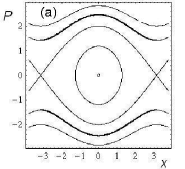
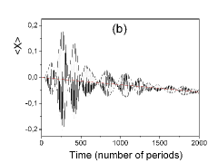
Figure 1: (a) Phase portrait of the unperturbed Hamiltonian and the initial distribution of particles (two segments of trajectories drawn in bold thick curves). (b) Drift of the average position of ensembles of particles with time in the potential $U(x)=-\cos x$ under the bichromatic perturbation described in the main text. We integrate 100 ensembles of particles, each ensemble contains 200 particles being distributed along two symmetric unperturbed trajectories with ${\cal{E}}_{0}=2.0$. Distribution is uniform in canonical ’angle’ variable of the unperturbed Hamiltonian. To each ensemble, we apply a force $E(t-t_{i})$, where $t_{i}$ is distributed uniformly on $(0,2\pi)$. Averaging over all ensembles gives us the average position $\bar{x}(t)$ (for convenience, a normalized position $\langle X\rangle=\bar{x}/2\pi\epsilon$ is shown, where the normalization is such that the slope of $\langle X\rangle(t)$, with time measured in units of fast periods, gives the average velocity). The inverse frequency $\epsilon=0.03$. After a certain transient period with beating oscillations of the average positions, the asymptotic regime is established.

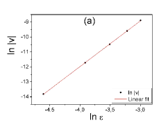
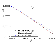
Figure 2: (a)Dependence of the average drift velocity on the inverse frequency $\epsilon$ for $U(x)=-\cos x$ and the perturbation described in the main text. Linear fitting give the coefficient $\alpha=3.05$ for the power-law $\ln|v|=\alpha\ln\epsilon$. Deviation from the asymptotic value $\alpha=3.0$ is partly due to the higher-order terms which are not so small in this range of $\epsilon$. (b) Average velocity as a function of $\epsilon^{3}$. Squares: integral formula of Eq. (Directed transport in a classical lattice with a high-frequency driving). Circles: numerical results. Triangles: asymptotic formula of Eq. (Directed transport in a classical lattice with a high-frequency driving). Lines are guides to the eye. Numerical results and the integral formula are almost indiscernible at this scale. The asymptotic formula deviates from numerics at larger values of $\epsilon$, where higher order terms become significant.

Numerically, we prepare a symmetric distribution of initial conditions in the phase space of the unperturbed Hamiltonian, and (abruptly) apply the force with an offset $t_{i}$. Applying the time-dependent force $E(t-t_{i})$, it is important to average over the initial phase $t_{i}$. Otherwise, one can obtain directed transport even in the case of harmonic driving Flach2 , as a function of the initial phase. In detail, our procedure is as follows. We prepare $N$ copies of a symmetric in coordinate and momentum initial phase-space distribution. Specifically, we choose as an initial distribution a collection of phase points distributed over two symmetric trajectories of the unperturbed Hamiltonian with the energy ${\cal E}={\cal{E}}_{0}$. To each copy, we apply at $t=0$ a force with an initial offset $t_{i}$: $E_{i}(t)=E(t-t_{i})$, where $E_{i}(t)$ is the force acting on the $i-$th copy of the phase space, and $t_{i}$ is an offset uniformly distributed on $(0,2\pi)$. We average over all phase points in all $N$ copies of the phase space. In other words, we average not only over initial phase-space distribution, but also over initial phase of the force.

For a numerical example, we consider the potential $U(x)=-\cos x$ and the following perturbation: $E(t)=-V_{1}\sin t-2V_{2}\sin(2t+\pi/4),$ where $V_{1}=3,\quad V_{2}=0.8$. This corresponds to

$$f(t)=V_{1}\cos t+V_{2}\cos(2t+\pi/4),$$ (10)

and we have: $v_{1}(t)=V_{1}\sin t+\frac{V_{2}}{2}\sin(2t+\frac{\pi}{4}),\quad\langle v_{1}^{2}\rangle_{t}=\frac{V_{1}^{2}}{2}+\frac{V_{2}^{2}}{8},$ $\langle f^{3}\rangle_{t}=\frac{3V_{1}^{2}V_{2}}{4\sqrt{2}}.$ We distribute particles along the trajectory of the unperturbed Hamiltonian with ${\cal E}_{0}=2$.

In Table I, we compare the numerical results for the average velocity with predictions of the integral formula (Directed transport in a classical lattice with a high-frequency driving) and the asymptotic formula (Directed transport in a classical lattice with a high-frequency driving). In Fig.1b, time evolution of the mean coordinate of ensembles of particles is shown for $\epsilon=0.03$. Slope of the fitted line gives the average velocity. In Fig.2a, the dependency of the average drift velocity on $\epsilon$ is shown. Note that the velocity is defined using ’old’, original time. In Fig. 2b, predictions of the integral formula (Directed transport in a classical lattice with a high-frequency driving), the asymptotic formula (Directed transport in a classical lattice with a high-frequency driving) and numerical calculations are compared.

Table 1: Average velocity from numerics and theory

$\epsilon$	Numerical result	Integral Eq. (Directed transport in a classical lattice with a high-frequency driving)	Asymptotic Eq. (Directed transport in a classical lattice with a high-frequency driving)
0.01	-1.004 $\cdot 10^{-6}$	-1.002 $\cdot 10^{-6}$	-9.987 $\cdot 10^{-7}$
0.02	-8.130 $\cdot 10^{-6}$	-8.099 $\cdot 10^{-6}$	-7.990 $\cdot 10^{-6}$
0.03	-2.784 $\cdot 10^{-5}$	-2.781 $\cdot 10^{-5}$	-2.697 $\cdot 10^{-5}$
0.04	-6.782 $\cdot 10^{-5}$	-6.756 $\cdot 10^{-5}$	-6.392 $\cdot 10^{-5}$
0.05	-1.372 $\cdot 10^{-4}$	-1.364 $\cdot 10^{-4}$	-1.248 $\cdot 10^{-4}$

To conclude, we derive the formula for average velocity of particles in a periodic potential under the influence of an unbiased high-frequency force. The average velocity is related to a certain integral momentum of the force, thereby the formula is useful for a wide range of perturbations including (but not limiting to) bichromatic or multichromatic harmonic driving, anharmonic driving, etc. Moreover, it provides sufficient conditions for directed transport, thereby conditions based on symmetry of the driving only give necessary conditions of existence of directed transport. Conceptual aspects of the phenomenon are clarified now. Indeed, applying classical perturbation theory of the 4-th order, one obtains an effective time-independent Hamiltonian. Although the Hamiltonian is symmetric in momentum, drift of particles occurs because the canonical transformation leading to the new Hamiltonian asymmetrically transforms original particle distribution into the distribution of particles in the new variables. A priori, it was not clear that mechanism of transport should be like this. In higher orders of the perturbation theory, one obtains an effective Hamiltonian with asymmetry in momentum Semenova . It might be possible that this asymmetry would be responsible for the transport, which is shown not to be the case: generally, transport arises within the 4th order of the perturbation theory. Importantly, the effective Hamiltonian does not possess chaotic dynamics. The full Hamiltonian has only a narrow stochastic layer on its phase space in the vicinity of the separatrix of unperturbed Hamiltonian. This layer becomes exponentially small in the high-frequency limit and cannot be described in any finite order of the perturbation theory. Since we consider energies not very close to the separatrix, this chaotic layer is completely irrelevant for the dynamics. In other words, chaos is not needed for the directed transport.

Procedure of the averaging used in our work is very important in the high-frequency case. Without averaging over the initial phase, it is not possible to catch the non-trivial part of the transport. That is, considering perturbation with a fixed initial phase and averaging only over the phase space, one gets directed transport even with the simple perturbation $E(t)=\cos(\omega t-\phi_{0})$. So far, experiments Renzoni only probed transport at fixed initial phase of the perturbation RenzoniPlus . We here reveal essential features of the nonlinear transport in the high-frequency regime that has not been probed in the experiments yet, and develop analytical theory for them. The theory can be probed in the experiments similar to Renzoni , but with a high-frequency perturbation. Our work can therefore inspire new experiments in this field.

This work was supported in part by RFBR 09-01-00333 and NSh-2519.2012.1 grants. The authors are grateful to L.Semenova for participation in the research on early stages, and to C. Petri, I.Brouzos, C.Morfonios, S.Flach, P.Schmelcher for useful discussions.

Supplementary information

We expand the effective Hamiltonian in series in $\epsilon$:

$${\cal H}(\bar{p},\bar{x},\epsilon) = {\cal H}_{0}(\bar{p},\bar{x})+\epsilon{\cal H}_{1}(\bar{p},\bar{x})+..$$

$$= {\cal H}(\bar{p},x+\epsilon^{2}\frac{\partial S}{\partial p},\epsilon)$$

$$= {\cal H}_{0}(\bar{p},x)+\frac{\partial{\cal H}_{0}}{\partial x}\Bigl{(}\epsilon^{2}\frac{\partial S_{1}}{\partial p}+\epsilon^{3}\frac{\partial S_{2}}{\partial p}+..\Bigr{)}+$$

$$+ \frac{1}{2}\frac{\partial^{2}{\cal H}_{0}}{\partial x^{2}}\Bigl{(}\epsilon^{2}\frac{\partial S_{1}}{\partial p}+\epsilon^{3}\frac{\partial S_{2}}{\partial p}+..\Bigr{)}^{2}+..$$

$$+ \epsilon{\cal H}_{1}(\bar{p},x)+\epsilon\frac{\partial{\cal H}_{1}}{\partial x}\Bigl{(}\epsilon^{2}\frac{\partial S_{1}}{\partial p}+\epsilon^{3}\frac{\partial S_{2}}{\partial p}+..\Bigr{)}+$$

$$+ \frac{1}{2}\epsilon\frac{\partial^{2}{\cal H}_{1}}{\partial x^{2}}\Bigl{(}\epsilon^{2}\frac{\partial S_{1}}{\partial p}+\epsilon^{3}\frac{\partial S_{2}}{\partial p}+..\Bigr{)}^{2}+..$$

$$+ \epsilon^{2}{\cal H}_{2}(\bar{p},x)+\epsilon^{2}\frac{\partial{\cal H}_{2}}{\partial x}\Bigl{(}\epsilon^{2}\frac{\partial S_{1}}{\partial p}+\epsilon^{3}\frac{\partial S_{2}}{\partial p}+..\Bigr{)}..$$

On the other hand, the effective and the intermediate Hamiltonians are related as

$${\cal{H}}(\bar{p},\bar{x},\epsilon) = H(p,x,t,\epsilon)+\epsilon\frac{\partial S}{\partial t}$$

$$= H_{0}(p,x,t)+\epsilon(H_{1}(p,x,t)+\frac{\partial S_{1}}{\partial t})$$

$$+ \epsilon^{2}(H_{2}(p,x,t)+\frac{\partial S_{2}}{\partial t})+..$$

$$= H_{0}(\bar{p},x,t)+\frac{\partial H_{0}}{\partial p}\Bigl{(}\epsilon^{2}\frac{\partial S_{1}}{\partial x}+\epsilon^{3}\frac{\partial S_{2}}{\partial x}+...\Bigr{)}$$

$$+ \frac{1}{2}\frac{\partial H_{0}^{2}}{\partial p^{2}}\Bigl{(}\epsilon^{2}\frac{\partial S_{1}}{\partial x}+\epsilon^{3}\frac{\partial S_{2}}{\partial x}+..\Bigr{)}^{2}$$

$$+ \epsilon(H_{1}(\bar{p},x,t)+\frac{\partial S_{1}}{\partial t})+\epsilon\frac{\partial H_{1}}{\partial p}\Bigl{(}\epsilon^{2}\frac{\partial S_{1}}{\partial x}+..\Bigr{)}$$

$$+ ...$$

We have

$H=\frac{p^{2}}{2}+U(x)+\epsilon pf(t)+\epsilon^{2}\frac{f(t)^{2}}{2},\quad$ $H_{0}=\frac{p^{2}}{2}+U(x),\quad H_{1}=pf(t),\quad H_{2}=\frac{f(t)^{2}}{2}.$

The term $\frac{f(t)^{2}}{2}$ does not influence the dynamics and can be safely omitted.

Comparing terms of the same order in $\epsilon$, we have (bars over $p$ are omitted):
The zero-order terms in $\epsilon$:

$$\epsilon^{0}:\quad{\cal H}_{0}(p,x)=H_{0}(p,x)=\frac{p^{2}}{2}+U(x),$$

The first-order terms in $\epsilon$:

$$\epsilon^{1}:\quad{\cal H}_{1} = H_{1}+\frac{\partial S_{1}}{\partial t},\quad{\cal H}_{1}=p\langle f\rangle_{t}=0,$$ (13)

$$S_{1} = -pv_{1}(t),\quad v_{1}(t)=\{f\}.$$

The second-order terms:

$$\epsilon^{2}:\quad{\cal H}_{2} + \frac{\partial H_{0}}{\partial x}\frac{\partial S_{1}}{\partial p}=H_{2}+\frac{\partial S_{2}}{\partial t}+\frac{\partial H_{0}}{\partial p}\frac{\partial S_{1}}{\partial x},$$

$$\quad{\cal H}_{2} = 0,\quad S_{2}=-v_{2}(t)U^{\prime}(x),$$

$$v_{2}(t) = \{v_{1}\}$$ (14)

The third-order terms:

$$\epsilon^{3}:\quad{\cal H}_{3}=0,\quad S_{3}=pv_{3}(t)U^{\prime\prime}(x),\quad v_{3}(t)=\{v_{2}\}$$ (15)

The fourth-order terms :

$$\epsilon^{4}:\quad{\cal H}_{4} + \frac{\partial{\cal H}_{0}}{\partial x}\frac{\partial S_{3}}{\partial p}+\frac{1}{2}\frac{\partial^{2}{\cal H}_{0}}{\partial x^{2}}\Bigl{(}\frac{\partial S_{1}}{\partial p}\Bigr{)}^{2}$$

$$= \frac{\partial S_{4}}{\partial t}+\frac{\partial H_{0}}{\partial p}\frac{\partial S_{3}}{\partial x}+\frac{\partial H_{1}}{\partial p}\frac{\partial S_{2}}{\partial x}+\frac{1}{2}\frac{\partial H_{0}^{2}}{\partial p^{2}}\Bigl{(}\frac{\partial S_{1}}{\partial x}\Bigr{)}^{2},$$

$$\quad{\cal H}_{4} = (-\langle fv_{2}\rangle_{t}-\frac{1}{2}\langle v_{1}^{2}\rangle_{t})U^{\prime\prime}(x)=\frac{1}{2}\langle v_{1}^{2}\rangle_{t}U^{\prime\prime}(x).$$

References

- (1) P.Reimann, Phys. Rep. 361, 57 (2002); P.Hanggi, F.Marchesoni, Rev. Mod. Phys. 81, 387 (2009).
- (2) D.Turaev et al, Phys. Rev. E 77, 065201 (2008); V. Gelfreich et al., Phys. Rev. Lett. 106, 074101 (2011); S. Bolotin, D. Treschev, Nonlinearity 12, 365 (1999); N. Brannstrom, V. Gelfreich, Physica D 237, 2913 (2008).
- (3) G.Casati, Chaos 15, 015120 (2005); T.Prosen, D.K.Campbell, ibid, 15, 015117 (2005).
- (4) A.P. Itin, R. de la Llave, A.I.Neishtadt, A.A. Vasiliev, Chaos 12, 1043 (2002).
- (5) S.Flach, O.Yevtushenko, Y. Zolotaryuk, Phys. Rev. Lett. 84, 2358 (2000).
- (6) O.Yevtushenko, S.Flach, K. Richter, Phys. Rev. E 61, 7215 (2000).
- (7) N. Strohmaier et al, Phys. Rev. Lett 99, 220601 (2007); A. Alberti et al, Nat. Phys. 5, 547 (2009); A. Zenesini et al. 102, 100403 (2009); A. Eckardt et al, Europhys. Lett. 89, 10010 (2010).
- (8) M. Holthaus, Phys. Rev. Lett. 69, 351 (1992); J. Karczmarek, M.Scott, M.Ivanov, Phys. Rev. A 60, R4225 (1999); S. Longhi, Phys. Rev. B 77, 195326 (2008); C.E. Creffield, F.Sols, Phys.Rev.Lett. 103, 200601 (2009); G. Benenti et al., Phys. Rev. Lett. 104, 228901 (2010).
- (9) K.Kudo, T. Boness, T.S. Monteiro, Phys. Rev. A 80, 063409 (2009); K.Kudo, T.S. Monteiro, Phys. Rev. A 83, 053627 (2011).
- (10) A. Kolovsky, E. Gomez, H.J. Korsch, Phys. Rev. A 81, 025603 (2010).
- (11) V.I. Arnold, V.V. Kozlov, and A.I. Neishtadt, Mathematical aspects of classical and celestial mechanics (Third Edition, Springer, Berlin, 2006).
- (12) X. Leoncini, A.I. Neishtadt, A.A. Vasiliev, Phys. Rev. E 79, 026213 (2009).
- (13) L.Semenova, unpublished (bachelor thesis).
- (14) M. Schiavoni et al, Phys. Rev. Lett. 90, 094101 (2003).
- (15) In Renzoni a bichromatic perturbation of the form was considered ( is a phase modulation of an optical lattice in the experiment which is equivalent to the uniform force in the system we discuss). Experiments were done at moderate frequencies, comparable to the frequency of unperturbed system. In this regime chaos is important and our analysis does not apply. By increasing the frequency of perturbation, one enters the regular regime which we describe, where there is no mixing and it is necessary to average over the initial phase to get the nontrivial part of the transport (i.e., to consider with different ).