Performance Evaluation of the Random Replacement Policy for Networks of Caches

Abstract

The overall performance of content distribution networks as well as recently proposed information-centric networks rely on both memory and bandwidth capacities. In this framework, the hit ratio is the key performance indicator which captures the bandwidth / memory tradeoff for a given global performance.
This paper focuses on the estimation of the hit ratio in a network of caches that employ the Random replacement policy. Assuming that requests are independent and identically distributed, general expressions of miss probabilities for a single Random cache are provided as well as exact results for specific popularity distributions. Moreover, for any Zipf popularity distribution with exponent $\alpha>1$, we obtain asymptotic equivalents for the miss probability in the case of large cache size.
We extend the analysis to networks of Random caches, when the topology is either a line or a homogeneous tree. In that case, approximations for miss probabilities across the network are derived by assuming that miss events at any node occur independently in time; the obtained results are compared to the same network using the Least-Recently-Used discipline, already addressed in the literature. We further analyze the case of a mixed tandem cache network where the two nodes employ either Random or Least-Recently-Used policies. In all scenarios, asymptotic formulas and approximations are extensively compared to simulations and shown to perform very well. Finally, our results enable us to propose recommendations for cache replacement disciplines in a network dedicated to content distribution. These results also hold for a cache using the First-In-First-Out policy.

1 Introduction

Communication networks use an ever increasing amount of data storage to cache information in transit from a source to a destination. Data caching is an auxiliary function, where a given piece of data is temporarily stored into a memory. The cache might then be queried at any time to provide an object that is possibly stored in that memory. Caches are typically located downstream a bandwidth bottleneck, e.g., a communication link with limited bandwidth or a shared bus in a network of chips. This storage then allows to increase the throughput of the data path and to decrease the rate of congestion events.

Many communication networks fall into such a model: the Internet, Content Delivery Networks (CDNs), Peer-To-Peer (P2P) as well as networks on chips. In fact, the increasing amount of content delivered to Internet users has pushed the use of Web caching into communication models based on distributed caching such as CDNs. New information-centric network architectures [17, 22, 25] have been recently proposed in order to have built-in network storage as a fundamental element of the underlying communication model. Content storage becomes a fundamental resource in such networks, aiming at minimizing content delivery time under an ever increasing demand that cannot simply be satisfied by increasing link bandwidth. Moreover, the use of network storage, enabling one to cache content in order to bypass bandwidth bottlenecks, appears cost effective as memory turns out to be cheaper than transmission capacity.

One of the fundamental operations of a cache is defined by its replacement policy which determines the object to be removed from the cache when the latter is full. Many replacement policies are based on content popularity, with significant cost for managing the sorted lists. This is the case, in particular, for the Least Frequently Used (LFU) policy and more sophisticated variants based on it. On the contrary, Most Recently Used (MRU), Least Recently Used (LRU), First-In-First-Out (FIFO) and Random (RND) policies have the compelling feature to replace cached objects with constant delay $O(1)$. In-network storage, as envisaged in the new architectures mentioned above, may require packet-level caching at line rate; current high-speed routers running complex replacement policies might not, however, sustain such high line rates [26]. In this framework, the RND and FIFO policies can therefore be seen as presenting the least possible complexity. In fact, RND and FIFO requires less memory access per packet than LRU or MRU, and it has been shown [26] that this advantage is critical for sustaining high-speed caching with current memory technology.

In this paper, we address performance issues of caching networks running the RND replacement policy. We mainly focus on the analytical characterization of the miss probabilities under the Independent Request Model (IRM) assumptions when the number of available objects is infinite. We first provide exact formula for the miss rate in the case of a light-tailed distribution content popularity, namely geometric, and for specific Zipf popularity distributions. Proposition 1 then proves that when the popularity distribution follows a general power-law with decay exponent $\alpha>1$, the miss probability is asymptotic to $A\rho_{\alpha}C^{1-\alpha}$ for large cache size $C$, where constants $A$ and $\rho_{\alpha}$ depend on $\alpha$ only. In Proposition 2, we extend that result to miss probabilities conditioned by the object popularity rank.

A second major contribution of the paper is given by Proposition 29, where we evaluate the performance of network of caches under the RND policy, for both linear and homogeneous tree networks and asymptotically Zipf popularity distributions. An approximate closed formula for the miss probability across the network is provided and compared to corresponding estimates for LRU cache networks. The analysis is also extended to the mixed tandem cache network where one cache employs LRU and the other one uses RND. Note that the choice of FIFO replacement policy instead of RND does not impact any result.

The specific focus on Zipf distributions, or more generally power-law distributions, made in this paper is motivated by numerous studies on Internet object popularity, starting from the late 90’s experiments on World Wide Web documents ([2],[3]), the content stored in enterprises media servers ([9],[11]) and to recent studies on Internet media content ([7], [24]). While other content popularity distributions might be considered, we do not provide here a complete review of the literature on Internet content popularity characterization; the above references confirm the pertinence of Zipf distributions for studying caching performance.

The remainder of the paper is organized as follows. Section 2 presents related work on the analytical performance evaluation of caching systems. Section 3 analyzes the RND cache replacement policy and its comparison to LRU for a single cache; these analytical results are compared with exact numerical and simulation results in Section 4. Section 5 reports the approximate analysis of the network of RND caches for two topologies, namely the line and the tree. Numerical and simulation results for the network case are reported in Section 6. Section 7 further evaluates the tandem cache system with one LRU and one RND cache, using numerical and simulation results. Section 8 concludes the paper (several proofs are detailed in the Appendix).

2 Related Work

There is a significant body of work on caching systems and their associated replacement policies that we will not attempt to review thoroughly. Here we only report the literature focusing on the analytical characterization of the performance of such systems.

The most frequently analyzed replacement policy is LRU whose performance is evaluated considering the move-to-front rule, consisting in putting the latest requested object in front of a list; a miss event for a LRU cache with finite size takes place when the position (also referred to as search cost) of an object in the list is larger than that size. Under the Independent Request Model, [23] calculates the expected search cost and its variance for finite lists. An explicit formula is given in [4, 16] for the probability distribution of that cost; such a formula is, however, impractical for numerical evaluation in case of large object population and large cache size. Integral representations obtained in [13, 14] using the Laplace transform of the search cost function reduce the problem to numerical integration.

An asymptotic analysis of LRU miss probabilities [18] for Zipf and Weibull popularity distributions provides simple closed formulas. Extensions to correlated requests are obtained in [10, 20], showing that short term correlation does not impact the asymptotic results derived in [18]; the case of variable object sizes is also considered in [21]. The analytical evaluation of the RND policy has been first initiated by [15] for a single cache where the miss probability is given by a general expression. To the best of our knowledge, its application to specific popularity distributions has, however, not yet been envisaged together with its numerical tractability for large object population and cache size.

We are aware of few papers that address the issue of networks of caches. A network of LRU caches has been analyzed by [28] using the approximation for the miss probability at each node obtained in [12], and assuming that the output of a LRU cache is also IRM; miss probabilities can then be obtained as the solution of an iterative algorithm that is proved to converge. The results of [18] are extended in [6] to a two-level request process where objects are segmented into packets, when assuming that the LRU policy applies to packets. The analysis is applied to line and tree topologies with in-path caching. Moreover, [5] extends [6] when network links have finite bandwidth.

3 Single cache model

In this section, we address the single cache system with RND replacement policy, deriving analytic expressions of the miss probability together with asymptotics for large cache size. To avoid technical results at first reading, the reader may quickly go through the notation of Section 3.1 and directly skip to main results given in Propositions 1 and 2.

3.1 Basic results

Consider a cache memory with finite size which is offered requests for objects. If the cache size is attained and a request for an object cannot be satisfied (corresponding to a miss event), the requested object is fetched from the repository server and cached locally at the expense of replacing some other object in the cache. The object replacement policy is assumed to follow the RND discipline, i.e.whenever a miss occurs, the object to be replaced is chosen at random, uniformly among the objects present in cache.

We consider a discrete time system: at any time $t\in\mathbb{N}$, the $t$-th requested object requested from the cache is denoted by $R(t)\in\{1,2,...,N\}$, where $N$ is the total number of objects which can be possibly requested (in the present analysis, the set of all possible documents is considered to be invariant in time). We assume that all $N$ objects are ordered with decreasing popularity, the probability that object $r$ is requested being $q_{r}$, $1\leq r\leq N$. In the following, we consider the Independent Reference Model, where variables $R(t)$, $t\in\mathbb{N}$, are mutually independent and identically distributed with common distribution defined by

$$\mathbb{P}(R=r)=q_{r},\;\;\;1\leq r\leq N.$$

Let $C\leq N$ be the cache capacity and denote by $\mathcal{N}_{C}$ the set of all ordered subsets $\{j_{1},...,j_{C}\}$ with $1\leq j_{k}\leq N$, $k\in\{1,...,C\}$, and $j_{k}<j_{\ell}$ for $k<\ell$. Define the cache state at time $t\in\mathbb{N}$ by the vector $\mathbf{S}(t)$; $\mathbf{S}(t)$ may equal any configuration $\mathbf{s}=\{j_{1},...,j_{C}\}\in\mathcal{N}_{C}$. In the following, we let

$$G(C)=\sum_{\{j_{1},...,j_{C}\}\in\mathcal{N}_{C}}\;q_{j_{1}}...q_{j_{C}}$$ (1)

with $G(0)=1$. Let $M(C)$ finally denote the stationary miss probability calculated over all possibly requested objects.
It is shown [15] that the cache configurations $(\mathbf{S}(t))_{t\in\mathbb{N}}$ define a reversible Markov process with stationary probability distribution given by

$$\mathbb{P}(\mathbf{S}=\mathbf{s})=\frac{1}{G(C)}\prod_{j\in\mathbf{s}}q_{j},\;\;\mathbf{s}\in\mathcal{N}_{C};$$ (2)

moreover ([15], Theorem 4), probability $M(C)$ equals

$$M(C)=\frac{\displaystyle\sum_{\{j_{1},...,j_{C}\}\in\mathcal{N}_{C}}q_{j_{1}}...q_{j_{C}}\sum_{r\notin\{j_{1},...,j_{C}\}}q_{r}}{\displaystyle\sum_{\{j_{1},...,j_{C}\}\in\mathcal{N}_{C}}q_{j_{1}}...q_{j_{C}}}.$$ (3)

In [15], it is also shown that the cache configuration stationary probability distribution and miss rate probability are identical in the case of a FIFO cache, hence our results apply for the FIFO policy as well.

Expression (3) can be actually written in terms of normalizing constants $G(C)$ and $G(C+1)$ only; this will give formula (3) a compact form suitable for the derivation of both exact and asymptotic expressions for $M(C)$.

Lemma 3.1

The miss rate $M(C)$ is given by

$$M(C)=(C+1)\frac{G(C+1)}{G(C)}$$ (4)

with $G(C)$ defined in (1).

Proof 3.2.

Any state $\mathbf{s}=\{j_{1},...,j_{C}\}\in\mathcal{N}_{C}$ corresponding to a unique sequence $1\leq j_{1}<j_{2}<...<j_{C}\leq N$ with $1\leq j_{k}\leq N$, the denominator of (3) therefore equals $G(C)$. The numerator of (3) can in turn be expressed as

$$\sum_{1\leq j_{1}<...<j_{C}\leq N}q_{j_{1}}...q_{j_{C}}\sum_{r\notin\{j_{1},...,j_{C}\}}q_{j}$$

$$=\sum_{1\leq j_{1}<...<j_{C}\leq N}q_{j_{1}}...q_{j_{C}}$$

$$\times\left(\sum_{1\leq r<j_{1}}q_{r}+...+\sum_{j_{C-1}<r<j_{C}}q_{r}+\sum_{j_{C}<r\leq N}q_{r}\right)$$

$$=(C+1)\sum_{1\leq r<j_{1}<...<j_{C}\leq N}q_{r}q_{j_{1}}...q_{j_{C}}=(C+1)G(C+1)$$

and expression (4) of $M(C)$ follows

The latter results readily extend to the case when the total number $N$ of objects is infinite, since the series $\Sigma_{j\geq 1}q_{j}$ is finite. The calculation of coefficients $G(C)$, $0\leq C\leq N$, is now performed through their associated generating function $F$ defined by

$$F(z)=\sum_{0\leq C\leq N}G(C)z^{C},\;\;z\in\mathbb{C},$$

for either finite or infinite population size $N$ (as $M(C)\leq 1$, Lemma 3.1 entails that $G(C+1)/G(C)\leq 1/(C+1)$ and the ratio test implies that the power series defining $F(z)$ has infinite convergence radius). We easily obtain the second preliminary result.

Lemma 3.3.

The generating function $F$ is given by

$$F(z)=\prod_{1\leq r\leq N}\left(1+q_{r}z\right)$$ (5)

for all $z\in\mathbb{C}$.

Proof 3.4.

Expanding the latter product and using definition (1) readily provide the result

To further study the single cache properties, let $M_{r}(C)$ denote the per-object miss probability, given that the requested object is precisely $r\in\{1,...,N\}$. Defining

$$G_{r}(C)=\sum_{1\leq j_{1}<...<j_{C}\leq N,\;r\notin\{j_{1},...,j_{C}\}}\;q_{j_{1}}...q_{j_{C}}$$ (6)

with $G_{r}(0)=1$, we then have $M_{r}(C)=\mathbb{P}(r\notin\mathbf{S})$ so that (2) and (6) yield

$$M_{r}(C)=\frac{G_{r}(C)}{G(C)}.$$ (7)

Lemma 3.5.

The per-object miss probability $M_{r}(C)$ for given $r\in\{1,...,N\}$ can be expressed as

$$M_{r}(C)=1+\sum_{\ell=0}^{C-1}(-q_{r})^{C-\ell}\frac{G(\ell)}{G(C)}.$$ (8)

The stationary probability $q_{r}(2)$, $r\in\{1,...,N\}$, that a miss event occurs for object $r$ is given by

$$q_{r}(2)=\frac{M_{r}(C)}{M(C)}q_{r}$$ (9)

where $M(C)$ is the averaged miss probability.

Proof 3.6.

By definition (6), the generating function $F_{r}(z)$ of coefficients $G_{r}(C)$, $0\leq C\leq N$, is given by

$$F_{r}(z)=\frac{F(z)}{1+q_{r}z},\;\;z\in\mathbb{C}.$$ (10)

Expanding the latter ratio as a powers series of $z$ gives

$$G_{r}(C)=\sum_{\ell=0}^{C}(-q_{r})^{C-\ell}G(\ell)$$

and provides (8) after using definition (7) for $M_{r}(C)$. Besides, letting $\mathcal{M}$ denote a miss event, Bayes formula entails

$$q_{r}(2) =\mathbb{P}(R=r\;|\;\mathcal{M})=\mathbb{P}(R=r)\frac{\mathbb{P}(\mathcal{M}\;|\;R=r)}{\mathbb{P}(\mathcal{M})}=q_{r}\frac{M_{r}(C)}{M(C)}$$

hence relation (9)

If the popularity distribution has unbounded support, then $\lim_{r\uparrow+\infty}q_{r}=0$ and formula (8) implies that the per-object probability $M_{r}(C)$ tends to 1 as $r\uparrow+\infty$ for fixed $C$; (9) consequently entails

$$q_{r}(2)\sim\frac{q_{r}}{M(C)},\;\;\;r\uparrow+\infty.$$ (11)

For given $C$, asymptotic (11) shows that the tail of distribution $(q_{r}(2))_{r\in\mathbb{N}}$ at infinity is proportional to that of distribution $(q_{r})_{r\in\mathbb{N}}$. The distribution $(q_{r}(2))_{r\in\mathbb{N}}$ describes the output process of the single cache generated by consecutive missed requests; it will serve as an essential ingredient to the further extension of the single cache model to network cache configurations considered in Section 5.

3.2 First applications

Coefficients $G(C)$, $C\geq 0$, and associated miss probability $M(C)$ can be explicitly derived for some specific popularity distributions. In the following, the total population $N$ of objects is always assumed to be infinite.

Corollary 3.7

Assume a geometric popularity distribution $q_{r}=(1-\kappa)\kappa^{r-1}$, $r\geq 1$, with given $\kappa\in\;]0,1[$. For all $C\geq 0$, the miss rate equals

$$M(C)=\frac{1-\kappa}{1-\kappa^{C+1}}(C+1)\kappa^{C}.$$ (12)

Proof 3.8.

Using Lemma 3.3, $F$ is readily shown to verify the functional identity $F(z)=(1+(1-\kappa)z)F(\kappa z)$ for all $z\in\mathbb{C}$. Expanding each side of that identity in power series of $z$ and identifying identical powers provides the value of the ratio $G(C+1)/G(C)$, hence result (12) by (4)

Let us now assume that the popularity distribution follows a Zipf distribution defined by

$$q_{r}=\frac{A}{r^{\alpha}},\;\;r\geq 1,$$ (13)

with exponent $\alpha>1$ and normalization constant $A=1/\zeta(\alpha)$, where $\zeta$ is the Riemann’s Zeta function. We now show how explicit rational expressions for miss rate $M(C)$ can be obtained for some integer values of $\alpha$.

Corollary 3.9

Assume a Zipf popularity distribution with exponent $\alpha$. For all $C\geq 0$, the miss probability equals

$$M(C) =\displaystyle\frac{3}{2C+3} \mathrm{if} \;\;\alpha=2,$$

$$=\displaystyle\frac{45}{(4C+5)(4C+3)(2C+3)} \mathrm{if} \;\;\alpha=4,$$

$$=\displaystyle\frac{9!}{3!}\frac{(C+1)}{\displaystyle\prod_{4\leq j\leq 9}{(6C+j)}} \mathrm{if} \;\;\alpha=6,$$

Proof 3.10.

When $\alpha=2$, the normalization constant equals $A=1/\zeta(2)=6/\pi^{2}$. From the infinite product formula [1]

$$F(z)=\prod_{j\geq 1}\left(1+\frac{u^{2}}{\pi^{2}j^{2}}\right)=\frac{\sinh u}{u}$$

and expanding the left hand side into powers of $u^{2}=Az\pi^{2}$ gives the expansion $F(z)=\Sigma_{C\geq 1}G(C)z^{C}$ where

$$G(C)=(\pi^{2}A)^{C}/(2C+1)!,\;\;C\geq 0.$$

Computing then ratio (4) with the above expression of $G(C)$ then provides $M(C)=3/(2C+3)$, as claimed. The cases when $\alpha=4$ or $\alpha=6$ follow a similar derivation pattern

The formulas of Corollary 3.9 do not seem, however, to generalize for integer values $\alpha=2p$ with $p\geq 4$; upper bounds can be envisaged and are the object of further study.

As also suggested by Corollary 3.9, the cache size corresponding to a target miss probability should be a decreasing function of $\alpha$. This property is generalized in Section 3.3 where an asymptotic evaluation of $M(C)$ is provided for large cache size $C$ and any Zipf popularity distribution with real exponent $\alpha>1$.

3.3 Large cache approximation

The specific popularity distributions considered in Corollaries 3.7 and 3.9 show that $M(C)$ is of order $Cq_{C}$ for $C$. In the present section, we derive general asymptotics for probabilities $M(C)$ and $M_{r}(C)$ for large cache size and apply them to the Zipf popularity distribution.

We first start by formulating a general large deviations result (Theorem 3.11) for evaluating coefficients $G(C)$ for large $C$. To apply the latter theorem to the Zipf distribution (13), we then state two preliminary results (Lemmas 3.12 and 3.13) on the behavior of the corresponding generating function $F$ at infinity. This finally enables us to claim our central result (Proposition 1) for the behavior of $M(C)$ for large $C$.

Theorem 3.11.

(See Proof in Appendix A)
(i) Given the generating function $F$ defined in (5), equation

$$zF^{\prime}(z)=CF(z)$$ (14)

has a unique real positive solution $z=\theta_{C}$ for any given $C\geq 0$;
(ii) Assume that there exists some constant $\sigma>0$ such that the limit

$$\lim_{C\uparrow+\infty}e^{s\sqrt{C}}\frac{F(\theta_{C}e^{-s/\sqrt{C}})}{F(\theta_{C})}=e^{\sigma^{2}s^{2}/2}$$ (15)

holds for any given $s\in\mathbb{C}$ with $\Re(s)=0$ and that, given any $\delta>0$, there exists $\eta\in]0,1[$ and an integer $C_{\delta}$ such that

$$\sup_{\delta\leq\mid y\mid\;\leq\pi}\left|\frac{F(\theta_{C}e^{iy})}{F(\theta_{C})}\right|^{1/C}\leq\eta$$ (16)

for $C\geq C_{\delta}$. We then have

$$G(C)\sim\frac{\exp(H_{C})}{\sigma\sqrt{2\pi C}}$$ (17)

as $C$ tends to infinity, with $H_{C}=\log F(\theta_{C})-C\log\theta_{C}$.

Following Theorem 3.11, the asymptotic behavior of $M(C)$ can then be derived from (17) together with identity (4). This approach is now applied to the Zipf popularity distribution (13); in this aim, the behavior of the corresponding generating function $F$ is first specified as follows.

Lemma 3.12.

(See Proof in Appendix B)
For $\alpha>1$ and large $z\in\mathbb{C}\setminus\mathbb{R}^{-}$, $\log F(z)$ expands as

$$\log F(z)=\alpha(\rho_{\alpha}Az)^{1/\alpha}-\frac{1}{2}\log(Az)+S_{\alpha}+o(1)$$ (18)

with $A=1/\zeta(\alpha)$ and $S_{\alpha}$ depending on $\alpha$ only and

$$\rho_{\alpha}=\left(\frac{\pi/\alpha}{\sin(\pi/\alpha)}\right)^{\alpha},$$ (19)

Lemma 3.13.

(See Proof in Appendix C)
For $\alpha>1$ and large $C$, the unique real positive solution $\theta_{C}$ of equation (14) verifies

$$\theta_{C}=\frac{C^{\alpha}}{A\rho_{\alpha}}+C^{\alpha-1}r_{C}$$ (20)

with $r_{C}=A_{1}+O(C^{-1})$ with $A_{1}=\alpha/2\rho_{\alpha}A$ if $\alpha\neq 2$ and $r_{C}=O(\log C)$ if $\alpha=2$.

We can now state our central result.

Proposition 1.

For a Zipf popularity distribution with exponent $\alpha>1$, the miss probability $M(C)$ is asymptotic to

$$M(C)\sim\rho_{\alpha}Cq_{C}=\frac{A\rho_{\alpha}}{C^{\alpha-1}}$$ (21)

for large $C$, with prefactor $\rho_{\alpha}$ given in (19).
Prefactor $\rho_{\alpha}$ verifies $\lim_{\alpha\uparrow+\infty}\rho_{\alpha}=1$ and $\rho_{\alpha}\sim 1/(\alpha-1)$ as $\alpha\downarrow 1$.

Proof 3.14.

As verified in Appendix D, the conditions of Theorem 3.11 are satisfied for a Zipf distribution. Using asymptotics (18) and (20) of Lemmas 3.12 and 3.13 to explicit the argument $H_{C}$ in (17) for large $C$, we then have

$$H_{C} =\log F(\theta_{C})-C\log\theta_{C}$$

$$=\alpha(\rho_{\alpha}A\theta_{C})^{1/\alpha}-\frac{1}{2}\log(A\theta_{C})+S_{\alpha}+o(1)-$$

$$\;\;\;\;C\log\left[\frac{C^{\alpha}}{A\rho_{\alpha}}+C^{\alpha-1}r_{C}\right]$$

so that $H_{C+1}-H_{C}=-\alpha\log C+k+o(1)$ with constant $k=\log\rho_{\alpha}+\log A$. Coming back to definition (4) of $M(C)$, the latter estimates enable us to derive that

$$M(C) =(C+1)\frac{G(C+1)}{G(C)}\sim C\exp[H_{C+1}-H_{C}]$$

$$\sim C\frac{e^{k}}{C^{\alpha}}=\rho_{\alpha}\;C\;q_{C}$$ (22)

as claimed

Remark 3.15.

Proposition 1 provides asymptotic (21) for $M(C)$ under the weaker assumption that the popularity distribution $q_{r}$, $r\geq 1$, has a heavy tail of order $r^{-\alpha}$ for large $r$ and some $\alpha>1$, without being precisely Zipf as in (13). In fact, all necessary properties for deriving Lemmas 3.12 and 3.13 are based on that tail behavior only.

To close this section, we now address the asymptotic behavior of $M_{r}(C)$ defined in (7).

Proposition 2.

For any Zipf popularity distribution with exponent $\alpha>1$ and given the object rank $r$, the per-object miss probability $M_{r}(C)$ is estimated by

$$M_{r}(C)\sim\frac{\rho_{\alpha}r^{\alpha}}{C^{\alpha}+\rho_{\alpha}r^{\alpha}}$$ (23)

for large $C$, with prefactor $\rho_{\alpha}$ defined in (19).

Proof 3.16.

The generating function $F_{r}$ of the sequence $G_{r}(C)$, $C\geq 0$, being given by (10), apply Theorem 3.11 to estimate coefficients $G_{r}(C)$ for large $C$. Concerning condition (i), the solution $\eta=\eta_{C}$ to equation $\eta F^{\prime}_{r}(\eta)=CF_{r}(\eta)$ reduces to equation (14) for $\theta=\theta_{C}$ where the term $q_{r}\theta/(1+q_{r}\theta)$ has been suppressed; but suppressing that term does not modify the estimate for $\theta_{C}$ with large $C$ so that $\eta_{C}\sim\theta_{C}$. On the other hand, condition (ii) is readily verified by generating function $F_{r}$ and we then obtain

$$G_{r}(C)\sim\frac{G(C)}{1+q_{r}\theta_{C}}.$$ (24)

By Lemma 3.13, we have $\theta_{C}\sim C^{\alpha}/A\rho_{\alpha}$ for large $C$; definition (7) of $M_{r}(C)$ and estimate (24) with $q_{r}=A/r^{\alpha}$ give

$$M_{r}(C)=\frac{G_{r}(C)}{G(C)}\sim\frac{1}{1+q_{r}\theta_{C}}\sim\frac{\rho_{\alpha}r^{\alpha}}{C^{\alpha}+\rho_{\alpha}r^{\alpha}}$$ (25)

and result (23) follows

For any value $\alpha>1$, (23) is consistent with the fact that $M_{r}(C)$ is an increasing function of object rank $r$ and a decreasing function of cache size $C$.

3.4 Comparing RND to LRU

Let us now compare the latter results with the LRU replacement policy investigated in [14, 18]. Recall that, for a Zipf popularity distribution with exponent $\alpha>1$, the miss probability $M(C)$ for LRU is estimated by

$$M(C)\sim\lambda_{\alpha}Cq_{C}$$

for large $C$, with prefactor

$$\lambda_{\alpha}=\frac{1}{\alpha}\left[\Gamma\left(1-\frac{1}{\alpha}\right)\right]^{\alpha}$$ (26)

where $\Gamma$ is Gamma function ([18], Theorem 3). $\lambda_{\alpha}$ is estimated by

$$\lambda_{\alpha}\sim\frac{e^{\gamma}}{\alpha},\;\;\;\;\lambda_{\alpha}\sim\dfrac{1}{\alpha-1}$$

as $\alpha\uparrow+\infty$ and $\alpha\downarrow 1$, respectively ($\gamma$ is Euler’s constant and $e^{\gamma}\approx 1,781...$). In view of Proposition 1, comparing asymptotics for coefficients $\lambda_{\alpha}$ and $\rho_{\alpha}$ shows that the difference $\rho_{\alpha}-\lambda_{\alpha}$ tends to 1 as $\alpha\uparrow+\infty$, thus illustrating that LRU discipline performs better than RND for large enough $\alpha$ (it can be formally shown that $\rho_{\alpha}>\lambda_{\alpha}$ for all $\alpha>1$). This difference diminishes, however, for smaller values of $\alpha$ since $\rho_{\alpha}$ and $\lambda_{\alpha}$ behave similarly as $\alpha$ is close to 1 (see Figure 1). Apart from that limited discrepancy, both disciplines provide essentially similar performance levels in terms of miss probabilities for large cache sizes.

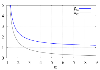
Figure 1: Prefactors $\rho_{\alpha}$ and $\lambda_{\alpha}$ with $\alpha>1$, for RND and LRU policies, respectively.

In contrast to heavy-tailed popularity distributions, we can consider a light-tailed distribution where

$$q_{r}=A\exp(-Br^{\beta}),\;\;r\geq 1,$$

with positive parameters $A,B,\beta$. It is shown in this case [18] that the miss probability for LRU is asymptotic to

$$M(C)\sim\frac{e^{\gamma}}{\beta B}C^{1-\beta}q_{C}$$

for large $C$. For a geometric popularity distribution (with $\beta=1$), the latter estimate shows that $M(C)=O(q_{C})$; on the other hand, formula (12) of Corollary 3.7 shows that $M(C)=O(Cq_{C})$ for RND discipline. This illustrates the fact that RND and LRU replacements provide significantly different performance levels if the popularity distribution is highly concentrated on a relatively small number of objects.

4 Numerical results: single cache

We here present numerical and simulation results to validate the preceding estimates for a single RND policy cache. In the following, when considering a finite object population with total size $N$, the Zipf popularity distribution is normalized accordingly. We also mention that the content popularity distribution obviously refers to document classes instead of individual documents. For comparison purpose with the existing LRU analysis, we represent these classes by a single index, as if they were a single document. In the following, cache sizes must accordingly be scaled up to the typical class size.

Simulations are performed using an ad-hoc simulator written in C. In every simulation, performance measures are collected after the transient phase, once the system has reached the stationary state. In this paper, transient behavior is not considered; note that the duration of the transient period obviously increases with the cache size.

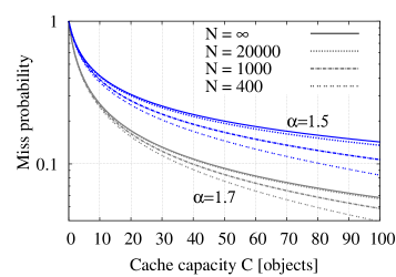
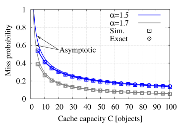
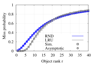
Figure 2: Single cache results: (a) exact formula for $M(C)$ with RND policy (b) asymptotic of $M(C)$ with RND policy (c) asymptotic of $M_{r}(C)$ with $C=25$, $\alpha=1.7$ for RND and LRU policies.

Besides, the most critical parameter in our simulation setting is the numerical value of $\alpha$. As the Zipf distribution flattens when $\alpha$ get closer to 1, much longer simulation runs are necessary to have good estimates of the miss rate. Small enough values of $\alpha$ must, nevertheless, be considered as they are more realistic. Estimates of $\alpha$ are reported, in particular, in [24] for web sites providing access to video content like www.metacafe.com for which $\alpha=1.43$, www.dailymotion.com and www.veoh.com for which $\alpha=1.72$ and $\alpha=1.76$, respectively. In the following, we hence fix $\alpha=1.5$ or $\alpha=1.7$ in our numerical experiments.

Fig. 2 first reports exact formula (3) for $M(C)=M(C;N)$ as a function of cache size $C$ and for increasing values of total population $N$, where $M(C;N)$ measures the total miss probability for a cache of size $C$ when the number of objects $N$ is finite. As expected, the convergence speed of $M(C;N)$ to $M(C;\infty)$ as $N\uparrow+\infty$ increases with $\alpha$. In the case $\alpha=1.5$ for instance, a population of $N=20\;000$ can be considered a good approximation for an infinite object population ($N=\infty$), whilst there is almost no difference between $M(C;N=20\;000)$ and $M(C;N=\infty)$ when $\alpha=1.7$.

In Fig. 2, we compare exact formula (3) for $M(C)$, asymptotic (21) and simulation results for the above scenario. Formula (3) for $N=\infty$ is computed with arbitrary precision and we used $N=20\;000$ for simulation as a good approximation for an infinite object population. Simulation and exact results are very close (especially for $\alpha=1.7$) while asymptotic (21) gives a very good estimation of the miss probability as soon as $C\geq 20$.

Fig. 2 presents the miss probability $M_{r}(C)$ as a function of the object rank $r$ for both RND and LRU policies with fixed $C=25$ and $\alpha=1.7$. Results are reported for the most popular classes and confirm the asymptotic accuracy of estimate (23) for RND and the corresponding one for LRU policy [19]. Beside the good approximation provided by the asymptotics, it is important to remark that RND and LRU performance are very close when object rank $r\geq 15$, while there is a slight difference for the most popular objects (say $r<15$). Moreover, comparing $M(C=25)$ for RND and LRU (respectively equal to 0.147 and 0.108), we observe only 4% less of miss probability using LRU with respect to RND policy. This may suggest RND as a good candidate for caches working at very high speed, where LRU may become too expensive in terms of computation due to its relative complexity.

5 In-network cache model

In order to generalize the single-cache model, networks of caches with various topologies can be considered.

5.1 Line topology

We first consider the tandem system defined as follows. Any request is addressed to a first cache $\sharp 1$ with size $C_{1}$; if it is not satisfied, it is addressed to a second cache $\sharp 2$ with size $C_{2}$:
- if this request is satisfied at cache $\sharp 2$, the object is copied to cache $\sharp 1$, with replacement performed according to the RND discipline;
- if this request is not satisfied at cache $\sharp 2$, the object is retrieved from a repository server and copied in caches $\sharp 1$ AND $\sharp 2$ according to the RND discipline.
Note that this replacement scheme, hereafter denoted by IPC for In-Path Caching, ignores any collaboration between the two caches and blindly copies objects in all caches along the path towards the requesting source.
We now fix some notation and properties for this tandem model. Let $R_{1}(t)\in\{1,2,...,N\}$ denote the object requested at cache $\sharp 1$ at time $t$; we still assume that variables $R_{1}(t)$, $t\in\mathbb{N}$, describe an IRM process with distribution defined by $\mathbb{P}(R_{1}=r)=q_{r}$, $1\leq r\leq N$. Denoting by $\mathbf{S}_{1}(t)$ (resp. $\mathbf{S}_{2}(t)$) the state vector of cache $\sharp 1$ (resp. $\sharp 2$) at time $t$, the bivariate process $(\mathbf{S}_{1}(t),\mathbf{S}_{2}(t))_{t\in\mathbb{N}}$ is easily shown to define a Markov process that, however, is not reversible. It is therefore unlikely that an exact closed form for the stationary distribution of process $(\mathbf{S}_{1},\mathbf{S}_{2})$ can be derived to evaluate the miss probability for the two-cache system.
Alternatively, we here follow an approach based on the approximation of the request process to cache $\sharp 2$. Let $t_{n}$, $n\in\mathbb{N}$, denote the successive instants when a miss occurs at first cache $\sharp 1$, and $R_{2}(n)$ be the object corresponding to that miss event at time $t_{n}$. First note that the common distribution of variables $R_{2}(n)$ is the stationary distribution $(q_{r}(2))_{r\in\mathbb{N}}$ introduced in Lemma 3.5, equation (9), with cache size $C$ replaced by $C_{1}$. In the following, we will further assume that

• the request process for cache $\sharp 2$ is an IRM, that is, all variables $R_{2}(n)$, $n\in\mathbb{N}$, are independent with common distribution

  $$\mathbb{P}(R_{2}=r)=q_{r}(2),\;\;r\in\mathbb{N}.$$

The simplifying assumption (H) neglects any correlation structure for the output process of cache $\sharp 1$ (that is, the input to cache $\sharp 2$) produced by consecutive missed requests. Recall also that the tail of distribution $(q_{r}(2))_{r\in\mathbb{N}}$, defined by (11), is proportional to that of distribution $(q_{r})_{r\in\mathbb{N}}$.

The latter 2-stage tandem model can be easily extended to a tandem network consisting in a series of $K$ caches ($K>2$) where any request dismissed at caches $\sharp 1,...,\sharp\ell$, $\ell\geq 1$, is addressed to cache $\sharp(\ell+1)$. As an immediate generalization of the IPC scheme, we assume that any requested document which experiences a miss at cache $\sharp j$, $1\leq j\leq\ell$, and an object hit at cache $\sharp(\ell+1)$ is copied backwards at all downstream caches $\sharp 1,...,\sharp\ell$. A request miss therefore corresponds to a miss event at each cache $1,2,...,K$. Furthermore, assumption (H) is generalized by saying that any cache $\sharp\ell$ considered in isolation behaves as a single cache with IRM input produced by consecutive missed requests at cache $\sharp(\ell-1)$. The size of cache $\sharp\ell$ is denoted by $C_{\ell}$.

In the following, the "global" miss probability $M_{r}(C_{1},\ldots,C_{\ell})$ (resp. "local" miss probability $M^{*}_{r}(C_{1},\ldots,C_{\ell})$) for request $r$ at cache $\ell$ is the miss probability for object $r$ over all caches $1,...,\ell$ (resp. the miss probability for object $r$ at cache $\ell$) so that

$$M_{r}(C_{1},\ldots,C_{\ell})=\prod_{j=1}^{\ell}M^{*}_{r}(C_{1},\ldots,C_{j})$$ (27)

(note that for a single cache, we have $M_{r}(C_{1})=M_{r}^{*}(C_{1})$). To simplify notation, we abusively write $M_{r}(\ell)$ (resp. $M^{*}_{r}(\ell)$) instead of $M_{r}(C_{1},\ldots,C_{\ell})$ (resp. instead of $M^{*}_{r}(C_{1},\ldots,C_{\ell})$). Finally, if $q_{r}(\ell)$, $r\geq 1$, defines the distribution of the input process at cache $\sharp\ell$, the averaged local miss probability $M^{*}(\ell)$ at cache $\sharp\ell$ is given by

$$M^{*}(\ell)=\sum_{r\geq 1}M_{r}^{*}(\ell)q_{r}(\ell)$$ (28)

for any $\ell\in\{1,...,K\}$.

Proposition 3.

(See Proof in Appendix E)
For the $K$-caches tandem system with IPC scheme, suppose that the request process at cache $\sharp 1$ is IRM with Zipf popularity distribution with exponent $\alpha>1$, and that assumption (H) holds for all caches $\sharp 2,...,\sharp K$.
For any $\ell\in\{1,...,K\}$ and large cache sizes $C_{1},...,C_{\ell}$, the global miss probability $M_{r}(\ell)$ (resp. local miss probability $M^{*}_{r}(\ell)$) is given by

$$M_{r}(\ell)\sim\frac{\rho_{\alpha}r^{\alpha}}{\displaystyle\rho_{\alpha}r^{\alpha}+\sum_{j=1}^{\ell}C_{j}^{\alpha}},\;\;\;M^{*}_{r}(\ell)\sim\frac{\displaystyle\rho_{\alpha}r^{\alpha}+\sum_{j=1}^{\ell-1}C_{j}^{\alpha}}{\displaystyle\rho_{\alpha}r^{\alpha}+\sum_{j=1}^{\ell}C_{j}^{\alpha}}.$$ (29)

Proposition 29 shows how the $K$-stage tandem system with IPC scheme improves the performance in terms of miss probability by adding a term $C_{j}^{\alpha}$ when the $j$-th cache is added to the path. From Propositions 29 and 1, it is readily derived that the average global miss probability $M(\ell)$ for all objects requested along the cache network is

$$M(\ell)=\sum_{r\geq 1}M_{r}(\ell)q_{r}\sim\frac{A\rho_{\alpha}}{\left(\displaystyle\sum_{j=1}^{\ell}C_{\ell}^{\alpha}\right)^{1-\frac{1}{\alpha}}}$$ (30)

for any $\ell\in\{1,...,K\}$ and large cache sizes $C_{1}$, …, $C_{\ell}$.

5.2 Tree topology

The previous linear network model can be easily extended to the homogeneous tree topology with Zipf distributed requests. By homogeneous, we mean that all leaves of the tree are located at a common depth of the root, and that the cache size for each node at a given level $i$ is equal to $C_{i}$ (where $C_{1}$ is the cache size of the leaves). An example of such a tree is a complete binary tree of given height.

Let $\Lambda_{1},\ldots,\Lambda_{J}$ be the $J$ leaves of the tree. We assume that all requests arrive at the leaves, following an IRM, that is, $\mathbb{P}(R(t)=r,\Lambda(t)=j)=p_{j}q_{r}$ for all $1\leq r\leq N$, $1\leq j\leq J$, where $\left(p_{1},\ldots,p_{J}\right)$ are positive values such that $\Sigma_{1\leq j\leq J}\;p_{j}=1$ and $\Lambda(t)$ denotes the leaf where the request $t$ arrives at time $t$. Requests are served according to the IPC rule, i.e., are forwarded upwards until the content is found, and the content is then copied in each cache between this location and the addressed leaf.

Corollary 5.1

Consider a homogeneous tree with IPC scheme and suppose that assumption (H) holds for all its internal nodes. The results of Proposition 29 then extend to that tree with IRM request process at leaves and Zipf popularity distribution with exponent $\alpha>1$.

Proof 5.2.

Only the order of requests in time matters since their precise timing is irrelevant; we can consequently assume that the requests arrive according to a Poisson process with intensity $1$. From the property of independent thinning and merging of Poisson processes, it follows that the requests for a given object $r$ at leaf $j$ is also a Poisson process of intensity $p_{j}q_{r}$, and that the request process at leaf $j$ is a Poisson process with intensity $p_{j}$ with a Zipf popularity distribution $q_{r}=A/r^{\alpha}$, $r\geq 1$. Now, using assumption (H) and applying the previous results for a single cache to each leaf, we deduce that at any leaf $j$, the miss sequence for object $r$ is a Poisson process with intensity $p_{j}q_{r}M_{r}^{*}(1)$. Merging these miss sequences from all children of a given second-level node, we deduce that the requests at this node follow a Poisson process and that the probability of request for an object $r$ is $q_{r}M_{r}^{*}(1)/M(1)=q_{r}(2)$. This process has the same properties as the IRM process with distribution $(q_{r}(2))_{r\in\mathbb{N}}$ used in the proof of Proposition 29, which therefore applies. Repeating recursively this reasoning at each level, we conclude that Proposition 29 holds in this context

Remark 5.3.

Corollary 5.1 is also valid for a homogeneous tree where different replacement policies are used at different levels $i$ (e.g. Random at first level and LRU at second one).

6 Numerical results: network of caches

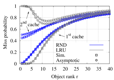
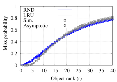
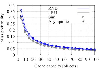
Figure 3: Tandem cache results: (a) asymptotics of $M^{*}_{r}(1)$, $M^{*}_{r}(2)$ (b) and of $M_{r}(2)$ for RND and LRU policies compared to simulation with $C_{1}=C_{2}=25$, $\alpha=1.7$ (c) Asymptotic for $M(2)=M(C_{1},C_{2})$ with $C_{1}=C_{2}\leq 100$, $\alpha=1.7$.

We here report numerical and simulation results to show the accuracy of the approximations presented in previous Section 5.

Fig. 3 first reports estimate (29) of $M_{r}^{*}(1)$ and $M_{r}^{*}(2)$ for both RND and LRU (the approximation for the tandem LRU are taken from [6]) with $C_{1}=C_{2}=25$. We focus on the second cache, as the performance of the first one has been largely analyzed in previous sections. We note a good agreement between the approximations evaluated in Section 5 and simulation results.

Moreover, while less popular objects are affected in the same way when employing either RND or LRU (in our specific example, $r\geq 15$), a significantly different behavior is detectable for popular objects ($r<15$). Local miss probabilities $M_{r}^{*}(1)$ and $M_{r}^{*}(2)$ help understanding where an object has been cached, conditioned on its rank. The combination of LRU and IPC clearly tends to favor stationary configurations where popular objects are likely to be stored in the first cache (see also [6] for a similar discussion). When using RND instead of LRU, however, the distribution of the content across the two caches is fairly different; in Fig. 3 for example, while the most popular objects are likely to be retrieved at the first cache when using either LRU or RND, only by using RND can such an object be also found in the second cache. It therefore appears that while both LRU and RND tend to store objects proportionally to their popularity, RND more evenly distributes objects across the whole path.

Fig. 3 reports the total miss probability at the second cache $M_{r}(2)=M^{*}_{r}(1)M^{*}_{r}(2)$, i.e., the probability to query an object of rank $r$ at the repository server. In this example, we see that objects with rank $r<15$ are slightly more frequently requested at the server when using RND rather than LRU, but RND is more favorable than LRU for objects with higher rank $r\geq 15$. In average, the total miss probability at the second cache $M(2)$, reported in Fig. 3, is very similar either using RND or LRU, with a slight advantage to LRU. $M(2)$ indicates the amount of data that is to be requested from the server.

With no claim of generality, we notice that the approximations calculated in Section 5 for RND and in [5], [6] for LRU are very accurate. Furthermore, the approximations work well for a large number of tests that we do not report here because of lack of space.

7 Mixture of RND and LRU

So far, we have considered networks of caches where all caches use the RND replacement policy. In practice, it is feasible to use different replacement algorithms in the same network. This section addresses the case of a tandem network, where one cache uses the RND replacement algorithm while the other uses the LRU algorithm. As in Section 5.2, these results also hold in the case of an homogeneous tree.

7.1 Large cache size estimates

We first provide estimates for miss probabilities in the case when cache sizes $C_{1}$ and $C_{2}$ are large.

Proposition 4.

For the $2$-caches tandem system with IPC scheme, suppose the request process at cache $\sharp 1$ is IRM with Zipf popularity distribution with exponent $\alpha>1$ and that assumption (H) for cache $\sharp 2$ holds.
I) When cache $\sharp 1$ (resp. cache $\sharp 2$) uses the RND (resp. LRU) replacement policy, the global (resp. local) miss probability $M_{r}(2)$ (resp. $M^{*}_{r}(2)$) on cache $\sharp 2$ is given by

$$M_{r}(2) \sim\frac{\rho_{\alpha}r^{\alpha}}{\displaystyle\rho_{\alpha}r^{\alpha}+C_{1}^{\alpha}}\exp\left(-\frac{\displaystyle\rho_{\alpha}C_{2}^{\alpha}}{\alpha\lambda_{\alpha}\left(\rho_{\alpha}r^{\alpha}+C_{1}^{\alpha}\right)}\right),$$

$$M^{*}_{r}(2) \sim\exp\left(-\frac{\displaystyle\rho_{\alpha}C_{2}^{\alpha}}{\alpha\lambda_{\alpha}\left(\rho_{\alpha}r^{\alpha}+C_{1}^{\alpha}\right)}\right)$$ (31)

for large cache sizes $C_{1}$, $C_{2}$ and constants $\rho_{\alpha}$, $\lambda_{\alpha}$ introduced in (19) and (26).
II) When cache $\sharp 1$ (resp. cache $\sharp 2$) uses the LRU (resp. RND) replacement policy, the global (resp. local) miss probability $M_{r}(2)$ (resp. $M^{*}_{r}(2)$) on cache $\sharp 2$ is given by

$$M_{r}(2) \sim\frac{\rho_{\alpha}r^{\alpha}}{\displaystyle\rho_{\alpha}r^{\alpha}\exp\left(\frac{C_{1}^{\alpha}}{\alpha\lambda_{\alpha}r^{\alpha}}\right)+C_{2}^{\alpha}},$$

$$M^{*}_{r}(2) \sim\frac{\rho_{\alpha}r^{\alpha}}{\displaystyle\rho_{\alpha}r^{\alpha}+C_{2}^{\alpha}\exp\left(-\frac{C_{1}^{\alpha}}{\alpha\lambda_{\alpha}r^{\alpha}}\right)}$$ (32)

for large cache sizes $C_{1}$, $C_{2}$.

Proof 7.1.

We follow the same derivation pattern as the proof of Proposition 29 detailed in Appendix E.
I) When cache $\sharp 1$ uses the RND replacement policy, we know from Appendix E that the request process at cache $\sharp 2$ is IRM with popularity distribution

$$q_{r}(2)=q_{r}\frac{M_{r}^{*}(1)}{M^{*}(1)}\sim\frac{C_{1}^{\alpha-1}}{C_{1}^{\alpha}+\rho_{\alpha}r^{\alpha}},\;\;r\geq 1,$$

and is asymptotically Zipf for large $r$. We then follow the proof of Proposition 6.2 of [6]. Let $S_{2}(0,t)$ be the number of different objects requested at cache $\sharp 2$ in the time interval $[0,t]$; it verifies

$$\mathbb{E}\left[S_{2}(0,t)\right]=\sum_{r\geq 1}\left(1-e^{-q_{r}(2)t}\right).$$

We then first deduce that

$$\mathbb{E}\left[S_{2}(0,t)\right]\geq\int_{1}^{+\infty}\left(1-e^{-q_{u}(2)t}\right)\mathrm{d}u.$$ (33)

Using the variable change $v=C_{1}^{\alpha-1}t/(C_{1}^{\alpha}+\rho_{\alpha}u^{\alpha})$ in the latter integral, we further obtain

$$\mathbb{E}\left[S_{2}(0,t)\right] \geq\left(\frac{C_{1}^{\alpha-1}t}{\rho_{\alpha}}\right)^{\frac{1}{\alpha}}\times$$

$$\int_{0}^{\frac{C_{1}^{\alpha-1}t}{C_{1}^{\alpha}+\rho_{\alpha}}}\frac{1}{\alpha}\left(1-e^{-v}\right)v^{-1-\frac{1}{\alpha}}\left(1-\frac{C_{1}v}{t}\right)^{\frac{1}{\alpha}-1}\mathrm{d}v\,.$$

Letting $t\uparrow+\infty$, the monotone convergence theorem for function $v\mapsto\left(1-C_{1}v/t\right)^{-1+1/\alpha}$ together with a further integration by parts yield

$$\lim_{t\uparrow+\infty}\frac{\mathbb{E}\left[S_{2}(0,t)\right]^{\alpha}}{t}\geq\left(\frac{C_{1}^{\alpha-1}}{\rho_{\alpha}}\right)\left[\Gamma\left(1-\frac{1}{\alpha}\right)\right]^{\alpha}.$$ (34)

Starting integral (33) from $u=0$ instead of $u=1$, the latter asymptotic bound is seen to hold also as an upper bound of $\mathbb{E}\left[S_{2}(0,t)\right]^{\alpha}/t$, thus showing that (34) actually holds as an equality. The local per-object miss rate on the second cache for an LRU cache is then

$$M_{r}^{*}(2) \sim\exp\left[-q_{r}(2)C_{2}^{\alpha}\left(\lim_{t\uparrow+\infty}\frac{\mathbb{E}\left[S_{2}(0,t)\right]^{\alpha}}{t}\right)^{-1}\right]$$

which proves expressions (31).
II) When cache $\sharp 1$ applies the LRU replacement policy, the local per-object miss rate at cache $\sharp 1$ is known [19] to equal

$$M_{r}^{*}(1)\sim\exp\left[-\frac{C_{1}^{\alpha}}{r^{\alpha}\left[\Gamma\left(1-\frac{1}{\alpha}\right)\right]^{\alpha}}\right]=\exp\left[-\frac{C_{1}^{\alpha}}{\alpha\lambda_{\alpha}r^{\alpha}}\right]$$

and that the local average miss rate is

$$M^{*}(1)\sim\frac{1}{\alpha}\left[\Gamma\left(1-\frac{1}{\alpha}\right)\right]^{\alpha}\frac{A}{C_{1}^{\alpha-1}}=\frac{\lambda_{\alpha}A}{C_{1}^{\alpha-1}}.$$

Using assumption (H), it then follows that the input process at cache $\sharp 2$ is IRM with popularity distribution given by

$$q_{r}(2)=q_{r}\frac{M_{r}^{*}(1)}{M^{*}(1)}\sim\frac{C_{1}^{\alpha-1}}{\lambda_{\alpha}r^{\alpha}}\exp\left[-\frac{C_{1}^{\alpha}}{\alpha\lambda_{\alpha}r^{\alpha}}\right],\;\;r\geq 1.$$

Note that this distribution is asymptotically Zipf for large $r$, with coefficient $A^{\prime}(2)=A/M^{*}(1)$. Applying estimate (25) to the above defined distribution $q_{r}(2)$, $r\geq 1$, it then follows that

$$M_{r}^{*}(2)\sim\left(1+q_{r}(2)\theta^{\prime}(2)\right)^{-1},$$

where the associated root $\theta^{\prime}(2)$ is easily estimated by $\theta^{\prime}(2)=C_{2}^{\alpha}/A^{\prime}(2)\rho_{\alpha}$ by using Lemma 3.13. We hence derive that

$$M_{r}^{*}(2)\sim\left(1+\displaystyle\frac{C_{2}^{\alpha}}{A^{\prime}(2)\rho_{\alpha}}\frac{AM_{r}^{*}(1)}{r^{\alpha}M^{*}(1)}\right)^{-1}$$

which leads to expressions (32)

7.2 Numerical results

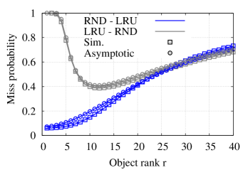
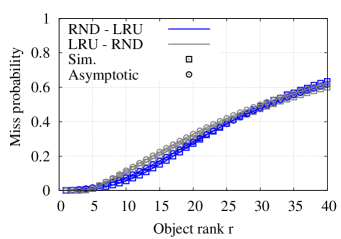
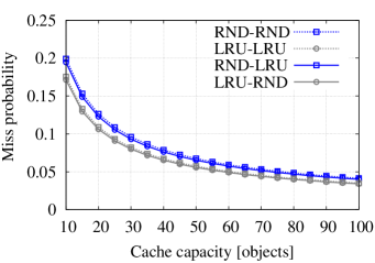
Figure 4: Mixed homogeneous tree cache results for mixed tree cache networks with $C_{1}=25,C_{2}=50$, $\alpha=1.7$: (a) asymptotic of $M^{*}_{r}(2)$ (b) asymptotic of $M_{r}(2)$ (c) Simulation of $M(2)=M(C_{1},C_{2})$ with $C_{1}=C_{2}\leq 100$, $\alpha=1.7$.

We here report numerical and simulation results for mixed homogeneous tree topologies to show the accuracy of the approximations presented in previous section, in order to derive some more general considerations about the mixture of RND and LRU in a network of caches. According to Section 5.2, we simulate in fact tree topologies, with 2 leaves with cache size $C_{1}$ and one root with cache size $C_{2}$.

Fig. 4 reports $M^{*}_{r}(2)$ for RND-LRU and LRU-RND homogeneous tree networks with asymptotics (31) and (32), respectively. We first note that the latter provide estimates with reasonable accuracy. Besides, we observe that the behavior of $M^{*}_{r}(2)$ is in strict relation to the policy used for cache $\sharp 1$. If cache $\sharp 1$ is RND then, $M^{*}_{r}(2)$ has a behavior similar to that observed in RND caches tandem; similarly, if cache $\sharp 1$ is LRU, $M^{*}_{r}(2)$ behaves as in the case of LRU caches in tandem.

This phenomenon has a natural explanation. RND and LRU act in the same way on objects ranked in the tail of the Zipf popularity distribution. However, the two replacement policies manage popular objects in a rather different way, as we already observed in Section 6. The second level caches see a local popularity that is shaped, by the first level of caches, in the body of the probability distribution. The portion of the distribution that is affected by such shaping process is determined by the cache size $C_{1}$ at first level. In the analysis reported in Fig. 4, the first level cache significantly determines the performance of the overall tandem system. In Fig. 4, we observe that the total miss probability $M_{r}(2)$ in the two mixed tandem caches is similar, while the distribution of the objects across the two nodes varies considerably.

Finally, in Fig. 4 we present simulation results of $M(2)=M(C_{1},C_{2})$ for all possible configurations in an homogeneous tree network in which $C_{1}=C_{2}\leq 100$. Observe that LRU-RND tree cache network achieve slightly better performance than the LRU-LRU system at least with Zipf shape parameter $\alpha=1.7$. This behaviour would suggest to prefer LRU at the first cache beacuse it performs better in terms of Miss probability and RND at the second one in order to save significant processing time.

8 Conclusion

The recent technological evolution of memory capacities, as illustrated by the deployment of CDNs and the proposition of new information-centric architectures where caching becomes an intrinsic network property, raise new interests on caching studies.

In this paper, we have studied the RND replacement policy, where objects to be removed are chosen uniformly at random. Assuming that the content popularity follows a Zipf law with parameter $\alpha>1$, and that content requests are IRM, we prove that for large cache size $C$, the miss rate is asymptotically equivalent to $A\rho_{\alpha}C^{1-\alpha}$ (see Lemma 3.12 and Proposition 1). This shows that the difference between LRU and RND caches is independent of the cache size and only depends on coefficient $A\rho_{\alpha}$. These results are extended to typical network topologies, namely tandems and homogeneous trees, under the assumption that requests are IRM at any node. The case of mixed policies (RND at one network level and LRU at the other one) is also considered. Simulations show that the IRM assumption applied to network topologies is reasonable and that provided estimates are accurate.

Our results suggest that the performance of RND is reasonably close to that of LRU. As a consequence, RND is a good candidate for high-speed caching when the complexity of the replacement policy becomes critical. In the presence of a hierarchy of caches, caches at deep levels (i.e. access networks) typically serve a relatively small number of requests per second which can be easily sustained by a cache running LRU; LRU policy should consequently be implemented at the bottom level since it provides the best performance. Meanwhile, higher-level caches see many aggregated requests and should therefore use the RND policy which yields similar performance (as to second-level cache) while being less computationally expansive.

We have assumed in this paper that the parameter $\alpha$ of the Zipf distribution is larger than $1$, and the total number of available objects is infinite. As an object of further study, we first intend to explore the case where $\alpha\leq 1$, with a finite number of objects. Besides, since Zipf popularity distributions do not represent all types of Internet traffic, we also intend to analyze the performance of RND caches when the content requests follow a light-tailed (e.g. Weibull) distribution. Finally, all results derived in this paper hold for i.i.d. content requests. Admittedly, actual traces show that requests are correlated, both in time and space. The definition of an accurate and realistic model which can take these correlations into account, as well as the extension of the present results to such a request model is also on our research agenda.

Appendix A Proof of Theorem 3.11

(i) Using (5), equation (14) reduces to $g(z)=C$ where

$$g(z)=z\frac{F^{\prime}(z)}{F(z)}=\sum_{j\geq 1}\frac{q_{j}z}{1+q_{j}z}.$$ (35)

Continuous function $g:z\in[0,+\infty[\;\rightarrow g(z)\in[0,+\infty[$ vanishes at $z=0$, is strictly increasing on $[0,+\infty[$ and tends to $+\infty$ when $z\uparrow+\infty$. Equation (14) has consequently a unique positive solution $\theta_{C}$. Note that $\theta_{C}$ tends to $+\infty$ with $C$ since $g(z)\leq\Sigma_{j\geq 1}(q_{j}z)=z$, hence $\theta_{C}\geq C$.
(ii) Consider the random variable $X_{C}$ with distribution

$$\mathbb{P}(X_{C}=x)=\frac{G(x)}{F(\theta_{C})}\theta_{C}^{x},\;\;x\geq 0,$$ (36)

where $\theta_{C}$ satisfies (14); note that definition (36) for $X_{C}$ is equivalent to

$$G(x)=\frac{F(\theta_{C})}{\theta_{C}^{x}}\mathbb{P}(X_{C}=x),\;\;x\geq 0.$$ (37)

Using definition (36), the generating function of random variable $X_{C}$ is $z\mapsto F(z\theta_{C})/F(\theta_{C})$; in view of (14), the expectation of variable $X_{C}$ is then

$$\mathbb{E}(X_{C})=\frac{\mathrm{d}}{\mathrm{d}z}\frac{F(z\theta_{C})}{F(\theta_{C})}\Big{|}_{z=1}=\theta_{C}\frac{F^{\prime}(\theta_{C})}{F(\theta_{C})}=C$$

so that random variables $Y_{C}=(X_{C}-C)/\sqrt{C}$, $C\geq 0$, are all centered. Besides, the Laplace transform of variable $Y_{C}$ is given by

$$\mathbb{E}(e^{-sY_{C}})=e^{s\sqrt{C}}\mathbb{E}(e^{-sX_{C}/\sqrt{C}})=e^{s\sqrt{C}}\frac{F(\theta_{C}e^{-s/\sqrt{C}})}{F(\theta_{C})}$$

for all $s\in\mathbb{C}$. By Lévy’s continuity theorem ([27], Theorem 4.2.4), assumption (15) entails that variables $Y_{C}$ converge in distribution when $C\uparrow+\infty$ towards a centered Gaussian variable with variance $\sigma^{2}$; moreover, assumption (16) ensures that the conditions of Chaganty-Sethuraman’s theorem ([8], Theorem 4.1) hold so that $\mathbb{P}(X_{C}=C)=\mathbb{P}(Y_{C}=0)$ is asymptotic to

$$\mathbb{P}(X_{C}=C)\sim 1/\sigma\sqrt{2\pi C}$$ (38)

as $C\uparrow+\infty$. Equation (37) for $x=C$ and asymptotic (38) together provide estimate (17) for $G(C)$ ∎

Appendix B Proof of Lemma 3.12

Let $q(x)=A/x^{\alpha}$ and $f_{z}(x)=\log(1+q(x)z)$ for any real $x\geq 1$ and $z\in\mathbb{C}$; definitions (5), (13) and the above notation then entail that

$$\log F(z)=\sum_{r\geq 1}f_{z}(r);$$

function $\log F$ is analytic in the domain $\mathbb{C}\setminus\mathbb{R}^{-}$. For given $z\in\mathbb{C}\setminus\mathbb{R}^{-}$ and integer $J\geq 1$, the Euler-Maclaurin summation formula [1] reads

$$\sum_{r=1}^{J}f_{z}(r)= \int_{1}^{J}f_{z}(x)\mathrm{d}x+\frac{1}{2}\left[f_{z}(J)+f_{z}(1)\right]+$$

$$\frac{1}{12}\left[f_{z}^{\prime}(J)-f_{z}^{\prime}(1)\right]+\frac{T_{z}(J)}{6}$$ (39)

with

$$T_{z}(J)=\int_{1}^{J}B_{3}(\{x\})f_{z}^{(3)}(x)\mathrm{d}x,$$

where $B_{3}(x)=x(x-1)(2x-1)/2$ is the third Bernoulli polynomial and $\{x\}$ denotes the fractional part of real $x$; derivatives of $f_{z}$ are taken with respect to $x$. Consider the behavior of the r.h.s. of (39) as $J$ tends to infinity. We first have $f_{z}(1)=\log(1+Az)$ and $f_{z}(J)=O(J^{-\alpha})$ for large $J$; differentiation entails

$$f_{z}^{\prime}(1)=-\frac{\alpha Az}{1+Az}$$

and $f_{z}^{\prime}(J)=O(J^{-\alpha-1})$ for large $J$. Differentiating twice again with respect to $x$ shows that the third derivative of $f_{z}$ is $O(x^{-\alpha-3})$ for large positive $x$, and is consequently integrable at infinity. Letting $J$ tend to infinity in (39) and using the above observations together with the boundedness of periodic function $x\geq 1\mapsto B_{3}(\{x\})$, we obtain

$$\log F(z)=\int_{1}^{+\infty}f_{z}(x)\mathrm{d}x+\frac{1}{2}\log(1+Az)+\frac{\alpha Az}{12(1+Az)}+\frac{T_{z}}{6}$$ (40)

where

$$T_{z}=\int_{1}^{+\infty}B_{3}(\{x\})f_{z}^{(3)}(x)\mathrm{d}x.$$ (41)

Now, considering the first integral in the r.h.s. of (40), the variable change $x=t(Az)^{1/\alpha}$ gives

$$\int_{1}^{+\infty}f_{z}(x)\mathrm{d}x =(Az)^{1/\alpha}\Big{[}L-\int_{0}^{1/(Az)^{1/\alpha}}\log\left(1+\frac{1}{t^{\alpha}}\right)\mathrm{d}t\Big{]}$$

$$=L(Az)^{1/\alpha}-\log(Az)-\alpha+o(1)$$ (42)

where $L$ is the finite integral [1]

$$L=\int_{0}^{+\infty}\log\left(1+\frac{1}{t^{\alpha}}\right)\mathrm{d}t=\frac{\pi}{\sin(\pi/\alpha)}=\alpha\rho_{\alpha}^{1/\alpha}$$ (43)

with $\rho_{\alpha}$ introduced in (19) for $\alpha>1$, and where

$$\int_{0}^{1/(Az)^{1/\alpha}}\log\left(1+\frac{1}{t^{\alpha}}\right)\mathrm{d}t=\frac{\log(Az)}{(Az)^{1/\alpha}}+\frac{\alpha}{(Az)^{1/\alpha}}+o(1).$$ (44)

Gathering (43) and (44) provides expansion (42). Using the explicit expression of $f^{(3)}_{z}$, the dominated convergence theorem finally shows that when $z\uparrow+\infty$, remainder $T_{z}$ in (41) tends to some finite constant $t_{\alpha}$ depending on $\alpha$ only. Gathering terms in (40)-(42), we are finally left with expansion (18) with constant $S_{\alpha}=-\alpha+\alpha/12+t_{\alpha}/6$. Some further calculations would provide $S_{\alpha}=-\alpha\log(2\pi)/2$, although this actual value does not intervene in our discussion ∎

Appendix C Proof of Proposition 3.13

Recall definition (35) of function $g$ and write equivalently

$$g(z)=\sum_{r\geq 1}g_{z}(r).$$

where we let $g_{z}(x)=Az(x^{\alpha}+Az)^{-1}$. The Euler-Maclaurin summation formula [1] applies again in the form

$$\sum_{r=1}^{J}g_{z}(r)= \int_{1}^{J}g_{z}(x)\mathrm{d}x+\frac{1}{2}\left[g_{z}(J)+g_{z}(1)\right]+$$

$$\frac{1}{12}\left[g_{z}^{\prime}(J)-g_{z}^{\prime}(1)\right]+\frac{W_{z}(J)}{6}$$ (45)

for given $z\in\mathbb{C}\smallsetminus\mathbb{R}^{-}$, integer $J\geq 1$ and where

$$\mid W_{z}(J)\mid\;\leq\frac{12}{(2\pi)^{2}}\int_{1}^{J}\mid g_{z}^{(3)}(x)\mid\mathrm{d}x$$

(derivatives of $g_{z}$ are taken with respect to variable $x$). Consider the behavior of the r.h.s. of (45) as $J$ tends to infinity. Firstly, $g_{z}(1)=Az/(Az+1)$ and $g_{z}(J)=O(J^{-\alpha})$ as $J\uparrow+\infty$; secondly, $g_{z}^{\prime}(1)=-A\alpha z(1+Az)^{-2}$ together with $g_{z}^{\prime}(J)=O(J^{-\alpha-1})$ for large $J$. Differentiating twice again shows that the third derivative of $g_{z}$ is $O(x^{-\alpha-3})$ for large positive $x$ and is consequently integrable at infinity. Letting $J$ tend to infinity in (45) therefore implies equality

$$g(z)=\int_{1}^{+\infty}g_{z}(x)\mathrm{d}x+\frac{1}{2}\frac{Az}{Az+1}+\frac{1}{12}\frac{A\alpha z}{(1+Az)^{2}}+\frac{W_{z}}{6}$$ (46)

where

$$\mid W_{z}\mid\;\leq\frac{12}{(2\pi)^{2}}\int_{1}^{+\infty}\mid g_{z}^{(3)}(x)\mid\mathrm{d}x.$$

Using the explicit expression of the derivative $g_{z}^{(3)}$, it can be simply shown that

$$\mid W_{z}\mid\;=O(z^{-2/\alpha}),\;\mid W_{z}\mid\;=O(z^{-1}\log z),\;\mid W_{z}\mid\;=O(z^{-1})$$ (47)

if $\alpha>2$, $\alpha=2$ and $1<\alpha<2$, respectively. Now, considering the first integral in the r.h.s. of (46), the variable change $x=t(Az)^{1/\alpha}$ gives

$$\int_{1}^{+\infty}g_{z}(x)\mathrm{d}x=I(Az)^{1/\alpha}-1+O\left(\frac{1}{z}\right)$$ (48)

where $I=L/\alpha=\rho_{\alpha}^{1/\alpha}$, with integral $L$ introduced in (43) for $\alpha>1$. Expanding all terms in powers of $z$ for large $z$, it therefore follows from (46) and (48) that

$$g(z)=\rho_{\alpha}^{1/\alpha}(Az)^{1/\alpha}-\frac{1}{2}+W_{z}$$

with $W_{z}$ estimated in (47). For large $C$, equation (35), i.e.$g(\theta_{C})=C$, then reads

$$A\theta_{C} =\left[\frac{C}{I}+\frac{1}{2I}+O(W_{\theta_{C}})\right]^{\alpha}$$

$$=\left(\frac{C}{I}\right)^{\alpha}+\frac{\alpha}{2I^{\alpha}}C^{\alpha-1}+O(C^{\alpha-2})$$ (49)

for $\alpha>2$ since (47) implies $W_{\theta_{C}}=O(\theta_{C}^{-2/\alpha})=O(C^{-2})$ in this case. The case $1<\alpha<2$ gives a similar expansion since the remainder is $W_{\theta_{C}}/C=O(C^{-\alpha}/C)=O(C^{-\alpha-1})$. Finally, the case $\alpha=2$ yields

$$A\theta_{C}=\left[\frac{C}{I}+\frac{1}{2I}+O(W_{\theta_{C}})\right]^{2}=\left(\frac{C}{I}\right)^{2}+O\left(\frac{\log C}{C}\right).$$ (50)

Gathering results (49)-(50) finally provides expansions (20) for $\theta_{C}$ ∎

Appendix D Proof of Proposition 1

We here verify that conditions (15) and (16) of Theorem 3.11 are satisfied in the case of a Zipf popularity distribution with exponent $\alpha>1$. Let us first establish convergence result (15). Using Lemma 3.12, we readily calculate

$$e^{s\sqrt{C}}\frac{F(\theta_{C}e^{-s/\sqrt{C}})}{F(\theta_{C})}=\;e^{s\sqrt{C}}\exp\Big{[}\alpha(\rho_{\alpha}A\theta_{C})^{1/\alpha}\times$$

$$\left(e^{-s/\alpha\sqrt{C}}-1\right)+\frac{s}{2\sqrt{C}}+\varepsilon(\theta_{C}e^{-s/\sqrt{C}})-\varepsilon(\theta_{C})\Big{]}$$ (51)

for any given $s\in\mathbb{C}$ with $\Re(s)=0$, $\mid\Im(s)\mid\;\leq a$ and where $\varepsilon(\theta)\rightarrow 0$ as $\theta\uparrow+\infty$. By Lemma 3.13, we further obtain $\alpha(\rho_{\alpha}A\theta_{C})^{1/\alpha}=\alpha C+\alpha\rho_{\alpha}r_{C}+o(r_{C})$ and the expansion of $e^{-s/\alpha\sqrt{C}}-1$ at first order in $1/C$ entails that

$$\alpha(\rho_{\alpha}A\theta_{C})^{1/\alpha}\left(e^{-s/\alpha\sqrt{C}}-1\right)=-s\sqrt{C}+\frac{s^{2}}{2\alpha}+O\left(\frac{1}{\sqrt{C}}\right);$$

letting $C$ tend to infinity, we then derive from (51) and the previous expansions that

$$e^{s\sqrt{C}}\frac{F(\theta_{C}e^{-s/\sqrt{C}})}{F(\theta_{C})}\rightarrow\exp\left(\frac{s^{2}}{2\alpha}\right)$$

so that assumption (15) is satisfied with $\sigma^{2}=1/\alpha$.
Let us finally verify boundedness condition (16). Rephrasing (51) for $s=-iy\sqrt{C}$, we have

$$\left(\frac{F(\theta_{C}e^{iy})}{F(\theta_{C})}\right)^{1/C}= \exp\Big{[}\frac{\alpha(\rho_{\alpha}A\theta_{C})^{1/\alpha}}{C}\left(e^{iy/\alpha}-1\right)-\frac{iy}{2C}$$

$$+\frac{\varepsilon(\theta_{C}e^{iy})-\varepsilon(\theta_{C})}{C}\Big{]}$$ (52)

for any $y\in\mathbb{R}$. But as above, $\alpha(\rho_{\alpha}A\theta_{C})^{1/\alpha}/C$ tends to the constant $\alpha$ when $C\uparrow+\infty$ so that

$$\left|\frac{F(\theta_{C}e^{iy})}{F(\theta_{C})}\right|^{1/C}\leq\mid h(y)\mid^{\beta}\times\Big{|}\exp\Big{[}\frac{\varepsilon(\theta_{C}e^{iy})-\varepsilon(\theta_{C})}{C}\Big{]}\Big{|}$$ (53)

for some positive constant $\beta$ and where

$$h(y)=\left|\exp\left(e^{iy/\alpha}-1\right)\right|=\exp\left(\cos\left(\frac{y}{\alpha}\right)-1\right).$$

Function $h$ is continuous, even and given $\delta>0$, $h$ is decreasing on interval $[\delta,\pi]$ since $\alpha>1$, hence $h(y)\leq h(\delta)=\eta_{\delta}<1$ for $\delta\leq y\leq\pi$. Using the estimates derived in Appendix B, it is further verified that, given any compact $\mathcal{K}\subset\mathbb{C}$ not containing the origin, we have $\lim_{C\uparrow+\infty}\varepsilon(\theta_{C}u)=0$ uniformly with respect to $u\in\mathcal{K}$; this entails that the exponential term in the right-hand side of (53) tends to 1 when $C\uparrow+\infty$ uniformly with respect to $u=e^{iy}$, $y\in[\delta,\pi]$. We finally conclude that condition (16) is verified ∎

Appendix E Proof of Proposition 29

Let $q_{r}(\ell+1)$, $r\geq 1$, denote the distribution of the input process at cache $\sharp(\ell+1)$, $\ell\geq 1$. By the same reasoning than that performed in Lemma 3.5, we can write

$$q_{r}(\ell+1)=q_{r}(\ell)\frac{M^{*}_{r}(\ell)}{M^{*}(\ell)}=q_{r}\frac{M^{*}_{r}(\ell)...M^{*}_{r}(1)}{M^{*}(\ell)...M^{*}(1)}$$ (54)

for all $r\in\mathbb{N}$, where $M^{*}_{r}(\ell)$ (resp. $M^{*}(\ell)$) is the local miss probability of a request for object $r$ at cache $\sharp\ell$ (resp. the averaged local miss probability for all objects requested at cache $\sharp\ell$) introduced in (28) and with notation $q_{r}=q_{r}(1)$. As $M_{r}^{*}(\ell^{\prime})\rightarrow 1$ for all $\ell^{\prime}\leq\ell$ when $r\uparrow+\infty$, we deduce from (54) that

$$q_{r}(\ell+1)\sim\frac{A(\ell)}{r^{\alpha}}$$

when $r\uparrow+\infty$, where $A(\ell)=A/M^{*}(1)M^{*}(2)...M^{*}(\ell)$. Apply then estimate (25) to obtain

$$M^{*}_{r}(\ell+1)\sim\frac{1}{1+\theta(\ell+1)q_{r}(\ell+1)}$$ (55)

where $\theta(\ell+1)\sim C_{\ell+1}^{\alpha}/A(\ell)\rho_{\alpha}$ and with $q_{r}(\ell+1)$ given by (54); using the value of $A(\ell)$ above and the definition $q_{r}=A/r^{\alpha}$, the product $\theta(\ell+1)q_{r}(\ell+1)$ reduces to

$$\theta(\ell+1)q_{r}(\ell+1) \sim\frac{C_{\ell+1}^{\alpha}}{A(\ell)\rho_{\alpha}}\cdot q_{r}\frac{M^{*}_{r}(\ell)...M^{*}_{r}(1)}{M^{*}(\ell)...M^{*}(1)}$$

$$=\frac{C_{\ell+1}^{\alpha}}{\rho_{\alpha}r^{\alpha}}M^{*}_{r}(\ell)...M^{*}_{r}(1).$$ (56)

Writing then $M_{r}(\ell+1)=M_{r}(\ell)M^{*}_{r}(\ell+1)$, asymptotics (55) and (56) together yield

$$M_{r}(\ell+1)\sim M_{r}(\ell)\left[1+\frac{C_{\ell+1}^{\alpha}}{\rho_{\alpha}r^{\alpha}}M^{*}_{r}(\ell)...M^{*}_{r}(1)\right]^{-1}$$

so that

$$\frac{1}{M_{r}(\ell+1)}\sim\frac{1}{M_{r}(\ell)}+\frac{C_{\ell+1}^{\alpha}}{\rho_{\alpha}r^{\alpha}}$$

since $\Pi_{j=1}^{\ell}M^{*}_{r}(j)=M_{r}(\ell)$ after (27); the latter recursion readily provides expression (29) for $M_{r}(\ell)$, $1\leq\ell\leq K$.
Using relation $M_{r}(\ell+1)=M_{r}(\ell)M^{*}_{r}(\ell+1)$ again together with expression (29) of $M_{r}(\ell)$ provides in turn expression (29) for $M^{*}_{r}(\ell)$, $1\leq\ell\leq K$ ∎

References

- [1] M. Abramowitz and I. Stegun. Handbook of Mathematical Functions with formulas, graphs and mathematical tables. Dover, 10th edition, 1972.
- [2] P. Barford, A. Bestavros, A. Bradley, and M. Crovella. Changes in web client access patterns: Characteristics and caching implications. World Wide Web, 2:15–28, January 1999.
- [3] L. Breslau, P. Cao, L. Fan, G. Phillips, and S. Shenker. Web caching and Zipf-like distributions: evidence and implications. In Proc. of IEEE INFOCOM, 1999.
- [4] J. Burville and J. F. C. Kingman. On a model for storage and search. Journal of Applied Probability, 10:697–701, September 1973.
- [5] G. Carofiglio, M. Gallo, and L. Muscariello. Bandwidth and storage sharing performance in information-centric networking. In Proc. of ACM SIGCOMM ICN, 2011.
- [6] G. Carofiglio, M. Gallo, L. Muscariello, and D. Perino. Modeling data transfer in content-centric networking. In Proc. of ITC23, 2011.
- [7] M. Cha, H. Kwak, P. Rodriguez, Y.-Y. Ahn, and S. Moon. I tube, you tube, everybody tubes: analyzing the world’s largest user generated content video system. In Proc. of ACM IMC, 2007.
- [8] N. R. Chaganty and J. Sethuraman. Multidimensional large deviations local limit theorems. Journal of Multivariate analysis, 20:190–204, 1986.
- [9] L. Cherkasova and M. Gupta. Analysis of enterprise media server workloads: access patterns, locality, content evolution, and rates of change. IEEE/ACM Transactions on Networking, 12(5):781 – 794, oct. 2004.
- [10] E. G. Coffman and P. R. Jelenković. Performance of the move-to-front algorithm with Markov-modulated request sequences. Operation Research Letters, 25(3):109–118, October 1999.
- [11] C. P. Costa, I. S. Cunha, A. Borges, C. V. Ramos, M. M. Rocha, J. M. Almeida, and B. Ribeiro-Neto. Analyzing client interactivity in streaming media. In Proc. of ACM WWW, 2004.
- [12] A. Dan and D. Towsley. An approximate analysis of the LRU and FIFO buffer replacement schemes. In Proc. of ACM SIGMETRICS, 1990.
- [13] J. A. Fill and L. Holst. On the distribution of search cost for the move-to-front rule. Random Structures and Algorithms, 8(3):179–186, 1996.
- [14] P. Flajolet, D. Gardy, and L. Thimonier. Birthday paradox, coupon collectors, caching algorithms and self-organizing search. Discrete Applied Mathematics, 39(3):207–229, 1992.
- [15] E. Gelenbe. A unified approach to the evaluation of a class of replacement algorithms. IEEE Transactions on Computer, 22(6):611–618, 1973.
- [16] W. J. Hendricks. The stationary distribution of an interesting Markov chain. Journal of Applied Probability, 9:231–233, 1972.
- [17] V. Jacobson, D. K. Smetters, J. D. Thornton, M. F. Plass, N. H. Briggs, and R. L. Braynard. Networking named content. In Proc. of ACM CoNEXT, 2009.
- [18] P. R. Jelenković. Asymptotic approximation of the move-to-front search cost distribution and least-recently-used caching fault probabilities. The Annals of Applied Probability, 9(2):430–464, 1999.
- [19] P. R. Jelenković and X. Kang. Characterizing the miss sequence of the LRU cache. ACM SIGMETRICS Performance Evaluation Review, 36:119–121, August 2008.
- [20] P. R. Jelenković and A. Radovanović. Least-recently-used caching with dependent requests. Theoretical Computer Science, 326(1–3):293–327, 2004.
- [21] P. R. Jelenković and A. Radovanović. Optimizing LRU caching for variable document sizes. Journal of Combinatorics, Probability and Computing, 13(4–5):627–643, 2004.
- [22] T. Koponen, M. Chawla, B.-G. Chun, A. Ermolinskiy, K. H. Kim, S. Shenker, and I. Stoica. A data-oriented (and beyond) network architecture. In Proc. of ACM SIGCOMM, 2007.
- [23] J. McCabe. On serial files with relocatable records. Operations Research, 12:609–618, July/August 1965.
- [24] S. Mitra, M. Agrawal, A. Yadav, N. Carlsson, D. Eager, and A. Mahanti. Characterizing web-based video sharing workloads. ACM Transactions on the Web, 5:8:1–8:27, May 2011.
- [25] Network of Information (NetInf). http://www.sail-project.eu/.
- [26] D. Perino and M. Varvello. A reality check for content-centric networking. In Proc. of ACM SIGCOMM ICN, 2011.
- [27] M. M. Rao and R. J. Swift. Probability Theory with Applications. Springer, 2nd edition, 2006.
- [28] E. J. Rosensweig, J. Kurose, and D. Towsley. Approximate models for general cache networks. In Proc. of IEEE INFOCOM, 2010.