Joint spectral-timing modelling of the hard lags in GX 339–4: constraints on reflection models

Abstract

The X-ray variations of hard state black hole X-ray binaries above 2 keV show ‘hard lags’, in that the variations at harder energies follow variations at softer energies, with a time-lag $\tau$ depending on frequency $\nu$ approximately as $\tau\propto\nu^{-0.7}$. Several models have so far been proposed to explain this time delay, including fluctuations propagating through an accretion flow, spectral variations during coronal flares, Comptonisation in the extended hot corona or a jet, or time-delays due to large-scale reflection from the accretion disc. In principle these models can be used to predict the shape of the energy spectrum as well as the frequency-dependence of the time-lags, through the construction of energy-dependent response functions which map the emission as a function of time-delay in the system. Here we use this approach to test a simple reflection model for the frequency-dependent lags seen in the hard state of GX 339–4, by simultaneously fitting the model to the frequency-dependent lags and energy spectrum measured by XMM-Newton in 2004 and 2009. Our model cannot simultaneously fit both the lag and spectral data, since the relatively large lags require an extremely flared disc which subtends a large solid angle to the continuum at large radii, in disagreement with the observed Fe K$\alpha$ emission. Therefore, we consider it more likely that the lags $>2$ keV are caused by propagation effects in the accretion flow, possibly related to the accretion disc fluctuations which have been observed previously.

1 Introduction

Black hole X-ray binaries (BHXRBs) have extensively been studied both in terms of their spectra (where a soft, multi-colour disc black-body and a harder power-law component play the main role) and in terms of their variability, which can be straightforwardly quantified using the common approach of computing the Power Spectral Density (PSD) of their signal. In combination with the time-averaged X-ray spectrum, this approach has enabled the variability to be studied as a function of spectral state, so that the hard power-law-dominated states can be associated with large variability amplitudes (tens of per cent fractional rms) and band-limited PSD shapes, while the soft disc-dominated states show much weaker variability and broadband power-law like PSD shapes.

Although they provide information on the global connection between the emitting components and the variability process, the PSD and mean energy spectra alone carry no information about the complex pattern of interlinkage between diverse regions in the accreting system that lead to transfer of variability from one physical component to another over a range of time-scales. In order to understand the causal connection between emission processes that show different relative strengths in two different energy bands, the time-lags between these two bands can be extracted as a function of Fourier frequency. To date, frequency-dependent lags have been studied mostly in the hard state of BHXRBs. There the lags ($\tau$) are ’hard’, in the sense that variations in harder bands lag behind variations in softer bands and depend on frequency as $\tau\propto\nu^{-0.7}$, albeit with some sharper ’steps’ in the lag-frequency relation (Miyamoto et al., 1988; Cui et al., 1997; Nowak et al., 1999). The general form of these lags has been explained by a variety of models, including Comptonisation in the extended corona (Kazanas et al., 1997) or a jet (Reig et al., 2003; Kylafis et al., 2008), spectral variability during coronal flares (Poutanen & Fabian, 1999), accretion fluctuations propagating through a power-law emitting region (e.g. a corona) with an energy-dependent radial emissivity profile (Kotov et al., 2001; Arévalo & Uttley, 2006), or light-travel times to an extended reflecting region (Kotov et al., 2001; Poutanen, 2002). Models invoking Comptonisation in the extended regions predict broader auto-correlation function for photons at higher energies, which suffer more scattering, which is opposite to what is observed (Maccarone et al., 2000; Poutanen, 2001).

Recent measurements of the lag (Uttley et al., 2011) between variations of the accretion disc blackbody emission and the power-law component strongly indicate that the variations are driven by fluctuations propagating through the disc (Lyubarskii, 1997) to the power-law emitting region, however this model cannot simply explain the hard lags between bands where the power-law dominates.

Models to generate frequency-dependent lags work by determining the response to an input signal of an emitting region which produces a hard spectral component, e.g. a compact coronal region sandwiching the disc, the upscattering region in the jet or an extended reflector. The input signal may be changes in the geometry, a fluctuation in accretion rate, seed photon illumination or illuminating primary continuum. The hard emitting region can only respond after a delay which, broadly speaking, is set by the time taken for the signal to propagate to and across the region. The delay time is determined by the signal speed (viscous time-scale or light-travel time) and the size scale of the hard emitting region. If the delay is large compared to the variability time-scale, the variations of the hard emitting region are smeared out and so the amplitude of variations of the lagging component is reduced. Thus the observed drop in lags with Fourier frequency can be reproduced.

In principle, models for the emitting regions which can reproduce the lags should also be able to reproduce the energy spectrum. Therefore, the combination of lag information with information on the X-ray spectral shape should provide much greater constraints on models for the emitting regions than either the commonly used spectral-fitting methods or the rarely-attempted fits to timing data. As a good proof-of-principle, the simplest models to attempt this joint lag and spectral-fitting are those where the lags are produced by reflection, i.e. so-called ‘reverberation’ lags. Evidence for small (few to tens of $R_{\rm g}$ light-crossing time) reverberation lags generated by reflection close to the black hole has been seen in Active Galactic Nuclei (Fabian & Ross, 2010; Zoghbi et al., 2010; de Marco et al., 2011; Emmanoulopoulos et al., 2011) and BHXRBs (Uttley et al., 2011), however the much larger lags we consider here require a larger scale reflector, perhaps from a warped or flaring outer-disc, which was originally considered by Poutanen (2002). Reflection of hard photons from a central corona off an accretion disc should produce both a reflection signature in the spectrum and a frequency-dependent time-lag, the shapes of which should depend on the exact geometry of the reflector as well as on the location of the corona itself (for a central, point-like corona, this would be the height above the disc). It has to be stressed that only non-flat disc geometries are expected to contribute a significant lag at low frequencies (Poutanen, 2002).

The CCD technology of the EPIC-pn camera onboard XMM-Newton provides a time resolution of 5.965 ms (frame readout time) in Timing mode with a 99.7% livetime and an energy resolution $\sim 125$ eV at 6 keV that combined, offer great potential for developing models that take into account energy and variability information together down to millisecond time-scales. Our aim in the present paper is to fit the spectra and time lags from an EPIC-pn Timing mode observation of a BHXRB simultaneously to discern whether reflection is the main driver of the observed hard-to-medium lags. In order to achieve this, we have developed reflags, a reflection model that assumes a flared accretion disc acting as reflector (assuming the constant density ionised disc reflection spectrum of Ballantyne et al. 2001), and is able to output for a given geometry either the resulting spectrum, or the expected lags as a function of frequency. We use this model to fit simultaneously the spectra and time-lags of the low-mass BHXRB GX 339–4 in the XMM-Newton observations of the hard state obtained in 2004 and 2009, and so determine whether the reflection model can explain the hard lags observed in these observations while also remaining consistent with the X-ray spectrum. In principle, this combined approach could yield much greater constraints on the outer disc geometry than can be obtained with spectral-fitting alone, since low velocities of the outer regions of the disc cannot be resolved with CCD detectors, although these regions should contribute significantly to the lags if they subtend a large solid angle as seen from the source.

We describe our model in Section 2 and the data reduction and extraction of spectra and time-lags in Section 3. In Section 4 we discuss the results from fitting the energy spectra and frequency-dependent time-lags of GX 339–4 together with our model, and also compare the expected optical/UV reprocessing signature of the inferred geometries with data from the Swift satellite. We discuss our results and the wider implications of our combined spectral-timing model-fitting approach in Section 5.

2 A flared accretion disc model

2.1 Model parameters

We consider a simple reflection model where the hard lags are produced by the light travel times from a variable power-law continuum source to the surface of a flared accretion disc which absorbs and reprocesses the incident radiation or scatters it producing a hard reflection spectrum (George & Fabian, 1991). Following the geometry described by Poutanen (2002), we have written reflags, an xspec model that can describe both the lags as a function of frequency and the mean spectrum, allowing simultaneous fitting by tying together the parameters from the spectral and lag fits. We assume that the accretion disc is axially symmetric but has a height of the disc surface above the mid-plane which depends on radius $r$ as a power-law

$$z(r)=H_{\rm out}\left(\frac{r}{R_{\rm out}}\right)^{\gamma},$$ (1)

where $H_{\rm out}$ is the height of the disc surface at the outermost radius $R_{\rm out}$ and $\gamma$ is the ‘flaring index’.

We place a point-like source of Comptonised photons at a certain height $H_{\textrm{src}}$ above the disc, located in the axis of symmetry of the system, and assume that the disc is truncated at some inner radius $R_{\rm in}$. Because the lags are proportional to the distances, while the spectral distortions due to rapid rotations are a function of radii in units of gravitational radius $R_{\rm g}=GM/c^{2}$, we have to specify the black hole mass, which we assume to be $M_{\rm BH}=10\mbox{M}_{\odot}$.

The amount of reflection of Comptonised photons that is expected to come from each region of the disc strongly depends on the value $\gamma$, and the only case where the contribution of outer radii to spectra and lags can be significant is for concave ($\gamma>1$) geometries (Poutanen, 2002).

The model also depends on the two parameters that describe the spectral shape: the incident power-law photon index $\Gamma$ and the ionisation parameter $\xi$. Due to computational constraints in the model evaluation, the latter is approximated to be constant throughout the disc. For computational purposes, the disc is also divided into 100 equally spaced azimuthal angles and 300 logarithmically spaced radii, to produce of a total of 30 000 cells.

The total energy-dependent power-law plus reflection luminosity per unit solid angle at a time $t$ that is emitted by a system whose geometry is described by the parameters above (represented by the set $\mathbf{\alpha}$) and seen at an inclination angle $i$ with respect to the axis of symmetry, equals:

$$\begin{split}L_{\rm tot}(E,t|\mathbf{\alpha},i)&=L_{\rm PL}(E,t)\\ &+a(E)\frac{\Omega_{\rm eff}}{2\pi}\sum_{l}L_{\rm PL}(E,t-\tau_{l})\kappa_{\mathbf{\alpha},l}(E,i),\end{split}$$ (2)

where the sum is performed over the index $l$ that represents a single disc cell, $L_{\rm PL}(E,t)$ is the luminosity per unit solid angle produced by power-law emission and $a(E)$ is the albedo function.

The factor $\kappa_{\mathbf{\alpha},l}(E,i)$ contains the several projection terms and solid angle corrections required for the $l$-th cell for the geometry described by $\mathbf{\alpha}$ (see Poutanen 2002), as well as relativistic Doppler and gravitational redshift corrections (following the same simplified approach as the diskline model, Fabian et al. 1989), and is normalised so that $\sum_{l}\kappa_{\mathbf{\alpha},l}(E,i)=1$. For a given geometry $\mathbf{\alpha}$ and inclination angle $i$, $\Omega_{\rm eff}$ then equals the solid angle subtended by the disc, corrected for the source inclination as seen by the observer. Finally, $\tau_{l}$ represents the time delay between observed direct power-law emission and reflected emission coming from the $l$-th cell.

2.2 System response and time-lags

For a direct power-law emission pulse (a delta-function) equation (2) can be rewritten as:

$$\begin{split}L_{\rm tot}(E,t|\mathbf{\alpha},i)&=L_{\rm PL}(E)\\ &\times\Big{(}\delta(t)+a(E)\frac{\Omega_{\rm eff}}{2\pi}\sum_{l}\kappa_{\mathbf{\alpha},l}(E,i)\delta(t-\tau_{l})\Big{)},\end{split}$$ (3)

and can be factorised as

$$L_{\rm tot}(E,t|\mathbf{\alpha},i)=L_{\rm PL}(E)T(E,t|\mathbf{\alpha},i),$$ (4)

where

$$T(E,t|\mathbf{\alpha},i)=\delta(t)+a(E)\frac{\Omega_{\rm eff}}{2\pi}\sum_{l}\kappa_{\mathbf{\alpha},l}(E,i)\delta(t-\tau_{l}).$$ (5)

The system response function $T(E,t|\mathbf{\alpha},i)$ contains the energy-dependent time redistribution of an input power-law luminosity as a function of time in a geometry $\mathbf{\alpha}$, as observed at an inclination $i$. Provided that the energy spectrum is averaged over a time significantly longer than the largest $\tau_{l}$, $\tau_{\rm max}$ (which in this case is of order 10 s), the spectrum is given simply given by: ${\rm const.}\times\int_{0}^{\tau_{\rm max}}T(E,t^{\prime}|\mathbf{\alpha},i){\rm d}t^{\prime}$. By taking the Fourier transform of equation (4):

$$\begin{split}\tilde{L}_{\rm tot}(E,\nu,i)&=\mathcal{F}\big{\{}L_{\rm PL}(E)T(E,t|\mathbf{\alpha},i)\big{\}}\\ &=L_{\rm PL}(E)\tilde{T}(E,\nu|\mathbf{\alpha},i).\end{split}$$ (6)

In general, the time-lags between two light curves $s(t)$ and $h(t)$ in the soft and hard bands can be calculated by computing their Fourier transforms $\tilde{S}(\nu)=\mathcal{F}[s(t)]$ and $\tilde{H}(\nu)=\mathcal{F}[h(t)]$ and forming the complex-valued quantity $C(\nu)=\tilde{S}^{*}(\nu)\tilde{H}(\nu)$, called the cross-spectrum (where the asterisk denotes complex conjugation). Its argument is the phase lag or phase difference between $\tilde{S}(\nu)$ and $\tilde{H}(\nu)$ (Nowak et al., 1999):

$$\phi(\nu)=\arg\big{[}C(\nu)\big{]}=\arg\big{[}\langle\tilde{S}^{*}(\nu)\tilde{H}(\nu)\rangle\big{]}$$ (7)

and therefore

$$\tau(\nu)=\frac{\phi(\nu)}{2\pi\nu}$$ (8)

equals the frequency-dependent time-lag.

The transfer function $\tilde{T}(E,\nu|\mathbf{\alpha},i)$ is equivalent to the response function $T(E,t|\mathbf{\alpha},i)$ in the Fourier-frequency domain. It is then possible to take the expression above to compute the cross-spectrum that will give the time-lags caused by reflection between two broad energy bands $s$ and $h$ and obtain the lags as above (the notation has been simplified):

$$C(\nu)=L_{\rm PL}(E_{\rm s})L_{\rm PL}(E_{\rm h})\tilde{T}^{*}(E_{\rm s},\nu)\tilde{T}(E_{\rm h},\nu),$$ (9)

$$\tau(\nu)=\frac{\arg\Big{[}\tilde{T}^{*}(E_{\rm s},\nu)\tilde{T}(E_{\rm h},\nu)\Big{]}}{2\pi\nu}.$$ (10)

3 Data reduction

3.1 Extraction of spectra, event files and instrumental response files

GX 339–4 was observed using the XMM-Newton X-ray satellite on 2004 March 16 and 2009 March 26 (ObsIds 0204730201 and 0605610201, respectively). In the present work, we will concentrate on the data taken using the EPIC-pn camera in Timing Mode, which allows for a fast readout speed, as opposed to imaging modes. This is done by collapsing all the positional information into one dimension and shifting the electrons towards the readout nodes, one macropixel row at a time, thus allowing a fast readout with a frame time of 5.965 ms (Kuster et al., 2002).

The raw Observation Data Files (ODFs) were obtained from the XMM-Newton Science Archive (XSA) and reduced using the XMM-Newton Science Analysis System version 10.0.0 tool epproc using the most recent Current Calibration Files (CCFs).

With the aid of evselect, the source event information was then filtered by column (RAWX in [31:45]), and pattern (PATTERN <= 4, corresponding to only single and double events), and only time intervals with a low, quiet background (where PI in [10000:12000]) were selected for the subsequent data analysis. The total exposure times are $\sim 164$ ks and $\sim 39$ ks for the 2004 and 2009 observations, respectively. The background spectrum was obtained from ObsId 0085680501 between columns 10 – 18 when the source was fainter so that the background is not contaminated by the source (see Done & Diaz Trigo (2010) for further details). rmfgen and arfgen were used to obtain the instrumental response files. To account for the effects of systematic uncertainties in the instrumentation, an additional 1% was added to the error bars.

In the present work, uncertainties in the estimation of the parameters are quoted at the 90% confidence level for one parameter of interest.

3.2 Extraction of the time-lags

When measuring the lags for real, noisy data one needs to first take the average of the cross-spectrum over many independent light curve segments (and also adjacent frequency bins). This is because observational noise adds a component to the cross-spectrum which has a phase randomly drawn from a uniform distribution (see e.g. Nowak et al. 1999). By averaging over many independent measures of the cross-spectrum, the contribution of these noise components can be largely cancelled out (the residual error provides the uncertainty in the lag). Therefore, the time-lags $\tau(\nu)$ were extracted from the argument of the cross spectrum averaged over many segments of the light curve as the exposure time and the dropouts due to telemetry saturation permit. Throughout this work we will take as the soft band the interval 2.0–3.5 keV and as a hard band the interval 4.0–10.0 keV.

We choose to have 8192 bins/segment for a total duration of $\sim 24.43$ seconds per segment, giving 6690 segments for 2004 and 1582 segments for 2009. This will also constrain the frequency ranges over which lags can be obtained. These frequencies have also been rebinned logarithmically with a step of $\Delta\ln\nu=0.14$ in order to improve the signal-to-noise per frequency bin.

The uncertainties on the lag measurements follow from the technique in Nowak et al. (1999) (see also Bendat & Piersol 2010). These scale as $\sqrt{NM}$ where $N$ is the number of segments used to average the cross-spectrum and $M$ is the number of frequencies averaged per bin. The lags are plotted on Fig. 1. Given the fact that, within the errors, the time-lag dependence on Fourier frequency is consistent between the two observations, we will sometimes assume that the time-lags for the two observations are equivalent and do not vary between the two observations as their shapes cannot be distinguished within the errors. This ‘substitution’ should in principle give us tighter constraints for our study in Section 4.

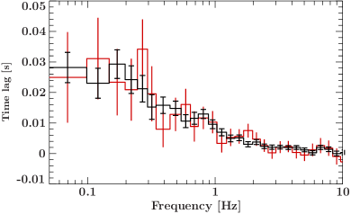
Figure 1: Time-lags between 4.0–10.0 and 2.0–3.5 keV energy bands as a function of frequency for the 2004 (black) and 2009 (red) observations.

4 Results

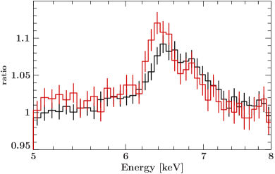
Figure 2: Ratio to a powerlaw after fitting the 2.0–5.0 keV and 7.0–10.0 keV continuum (black: 2004, red: 2009). The presence of the iron line is clear.

We test the model described in Section 2 using the 2004 and 2009 observations of GX 339–4, in order to understand the validity of the model and infer the geometrical parameters of the reflecting disc that is required to explain both the spectrum and the lags. To do this, the same model is concurrently fitted to the spectrum as well as the lag versus frequency data. Using this approach, it is possible to discern the importance of reflection to explain the observed lags, and whether or not an extra variability component to produce the lags is required.

In Fig. 2 we plot the ratio of the 2004 and 2009 spectra to a power-law fitted to the 2.0–10.0 keV interval excluding the region 5.0–7.0 keV. The iron line shape appears clearly different, with the 2004 dataset showing a more broadened profile that is skewed towards higher energies, while the 2009 line appears narrower and peaked at about 6.4 keV, the value expected for neutral or weakly-ionised emission.

We perform fits using the 2004 and 2009 spectra in the 3.0–10.0 keV band as well as their respective lags (we name these model fits A and B, respectively). These energy intervals are chosen in order to avoid contamination from the band dominated by the disc blackbody emission. Due to the small uncertainties on the spectral data, the weak steepening in spectral shape seen below 3 keV can skew the fit to the spectrum, hence we cut off the spectral fit at 3 keV. However, as shown by Uttley et al. (2011), the lags are not significantly affected by the disc at energies down to 2 keV, hence we include photons down to this energy in the lag determination, in order to increase signal-to-noise.

Parameter	Obs. A	Obs. B
$R_{\rm in}/R_{\rm g}$	$<130$	$<220$
$R_{\rm out}/R_{\rm g}$	$(16.8^{+2.4}_{-2.7})\times 10^{3}$	$(20^{+50}_{-8})\times 10^{3}$
$H_{\rm out}/R_{\rm out}$	$>0.83$	$>0.46$
$H_{\textrm{src}}/R_{\rm g}$	$>380$	$>330$
$\gamma$	$2.18^{+0.19}_{-0.24}$	$>1.69$
$i$	$39.7^{+0.4}_{-0.5}$	$29.8^{+1.8}_{-4.3}$
$\Gamma$	$1.481^{+0.003}_{-0.002}$	$1.468^{+0.004}_{-0.006}$
$\log\xi$	$2.05^{+0.03}_{-0.02}$	$2.03^{+0.02}_{-0.01}$
$\Omega^{\rm eff}/(2\pi)$	1.13	1.28
$\chi^{2}$ (spectrum)	1405	1305
$\chi^{2}$ (time-lags)	152	32
$\chi^{2}$/dof	1557 / 1417	1337 / 1416

Table 1: Spectral and lag fit parameters using the model reflags in the band 3–10 keV. Hereinafter, we quote the total $\chi^{2}$ as well as the contribution of the $\chi^{2}$ that corresponds to both the spectrum and lags, separately.

The best-fitting parameters for fits A and B are shown in Table 1. The corresponding model comparisons to the data, including the data-to-model ratios are plotted in Figs 3 and 4. These initial fits suggest that the model can represent the 2009 (B) data better. The upper limit on the disc inner radius is below 220 $R_{\rm g}$ in both cases. This value does not give us any information on whether the accretion disc in GX 339–4 is truncated or not (for discussions about disc truncation, see e.g. Tomsick et al. 2009).

As for the values of the outer radius, its value could reach up to $\sim 8\times 10^{4}$ $R_{\rm g}$ in B, much larger than what is found in A, indicating a larger contribution to the narrow iron line in this case. This is in agreement with the stronger core of the line in B as seen in the ratio plot (Fig. 2) as well as the difference between the solid angles. An extremely high value for the source height $H_{\rm src}$ and a high value for the $H_{\rm out}/R_{\rm out}$ ratio suggest that the fits are being driven by the lags, whose amplitude is strongly dependent on the distances to the furthest regions of the reflector, even if their contribution is small. The ionisation parameter remains consistent between the observations, although a visual inspection of the residuals and a clear difference in $\chi^{2}$ are indicative of a disc that can be described with a line of ionised iron, and whose contribution would likely come from the inner disc regions of the accretion disc where the ionisation could plausibly be larger. The blue wing of a relativistically broadened disc line could conceivably also contribute to the residuals which we fit with a narrow line, however since the inner disc radius is not strongly constrained by the lags, the model is already relatively free to fit this feature with relativistic emission, by being driven by the spectral data alone. The fact that it does not fit these residuals suggests that a more complex ionisation structure of the disc is likely (also see Wilkinson (2011)).

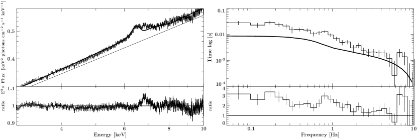
Figure 3: Obs. A (2004) spectrum (left) and lags vs frequency (right). The thick solid line represents the model for the best-fitting parameters (see Table 1, left column). In the spectrum, the thin solid line represents the direct continuum power-law. The lower panels show the ratio data/model.

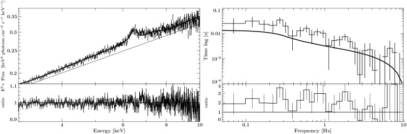
Figure 4: Obs. B (2009) spectrum (left) and lags vs frequency (right). The thick solid line represent the models reflags for the best-fitting parameters (see Table 1, right column).

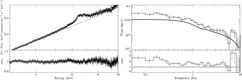
Figure 5: Obs. A (2004) spectrum (left) and lags vs frequency (right). The thick solid lines represent the model reflags (including a Gaussian component in the case of the spectrum) for the best-fitting parameters (see Table 2, left column).

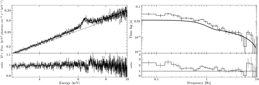
Figure 6: Obs. B’ (2009 spectrum, 2004 lags) spectrum (left) and lags vs frequency (right). The thick solid lines represent the model reflags for the best-fitting parameters (see Table 2, right column).

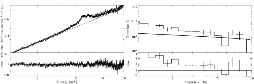
Figure 7: Obs. A (2004 spectrum (left) and lags vs frequency (right). The thick solid lines represent the model reflags (including a Gaussian component in the case of the spectrum) for the best-fitting parameters (see Table 3, left column), in the frequency range 1–10 Hz.

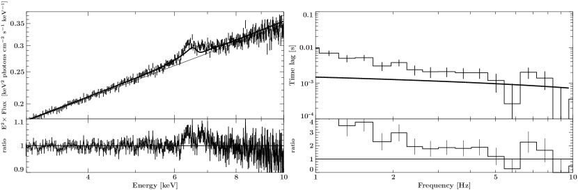
Figure 8: Obs. B’ (2009 spectrum, 2004 lags) spectrum (left) and lags vs frequency (right). The thick solid lines represent the model reflags for the best-fitting parameters (see Table 3, right column), in the frequency range 1–10 Hz.

However, as seen in the right panel of Fig. 3, the model is clearly under-predicting the lags that are observed by a factor of $\sim 2$, mainly at low frequencies that would correspond to a light-crossing time expected from distant reflection. Given that our focus is on the lags and our aim is to understand whether they are compatible with being caused by reflection, we test whether the lags are being constrained by the line shape by adding an extra Gaussian component of variable width to the spectral model for the 2004 data only, that corresponds to the dataset with higher signal-to-noise. In this way, we improve the fit ‘artificially’ so that the model can find the best-fitting contribution to the narrow 6.4 keV core which might originate at larger radii, and thus we allow the model more freedom to produce larger lags which better fit the data.

Parameter	Obs. A + extra line	Obs. B’
$R_{\rm in}/R_{\rm g}$	$<90$	$<120$
$R_{\rm out}/R_{\rm g}$	$(8.8^{+3.8}_{-1.6})\times 10^{3}$	$(11.0^{+2.6}_{-1.9})\times 10^{3}$
$H_{\rm out}/R_{\rm out}$	$0.84\pm 0.04$	$0.95^{+0.08}_{-0.14}$
$H_{\textrm{src}}/R_{\rm g}$	$430^{+90}_{-80}$	$>380$
$\gamma$	$2.22^{+0.21}_{-0.33}$	$2.62^{+0.36}_{-0.43}$
$i$	$48.9^{+1.0}_{-0.6}$	$42.3^{+1.3}_{-0.8}$
$\Gamma$	$1.479\pm 0.003$	$1.46\pm 0.05$
$\log\xi$	$1.50^{+0.12}_{-0.24}$	$1.65^{+0.08}_{-0.17}$
$E_{\rm c}$ [keV]	$6.92\pm 0.02$	$-$
$\sigma_{\rm c}$ [keV]	$0.17^{+0.03}_{-0.02}$	$-$
$\Omega^{\rm eff}/(2\pi)$	0.78	1.03
$\chi^{2}$ (spectrum)	1132	1335
$\chi^{2}$ (time-lags)	107	77
$\chi^{2}$/dof	1239 / 1414	1412 / 1417

Table 2: Spectral and lag fit parameters using the model reflags plus an extra Gaussian fitted to 2004 spectrum and lags (obs. A), and mixing the 2009 observation spectrum with the 2004 observation lags (obs. B’).

The best-fitting parameters after this procedure can be found in the first column of Table 2, and an improvement in $\chi^{2}$ is clear. The centroid energy for the additional emission line does not correspond to any ionised iron fluorescence transition, hence its value may come from a weighted mean of lines with a complex ionisation.

The decrease in the reflags solid angle is compatible with the addition of the extra line, i.e. the main model does not need to fit it anymore. Despite the attempt to artificially improve the spectral fit to allow the model to better fit the large scale reflection, the lags from the model are still too low (Fig. 5).

Parameter	Obs. A + extra line	Obs. B’
$R_{\rm in}/R_{\rm g}$	$<60$	$<22$
$R_{\rm out}/R_{\rm g}$	$(8.2^{+14.2}_{-3.6})\times 10^{3}$	$(9.1^{+12.2}_{-3.5})\times 10^{3}$
$H_{\rm out}/R_{\rm out}$	$>0.06$	$<0.05$
$H_{\rm src}/R_{\rm g}$	$>80$	$>80$
$\gamma$	$>1.1$	$>1.0$
$i$	$<31.0$	$<30.2$
$\Gamma$	$1.459\pm 0.003$	$1.4398^{+0.003}_{-0.009}$
$\log\xi$	$<1.34$	$<1.31$
$E_{\rm{c}}$ [keV]	$6.85\pm 0.02$	$-$
$\sigma_{\rm c}$ [keV]	$0.25\pm 0.03$	$-$
$\Omega^{\rm eff}/(2\pi)$	0.81	0.86
$\chi^{2}$ (spectrum)	1108	1449
$\chi^{2}$ (time-lags)	74	78
$\chi^{2}$/dof	1182 / 1402	1527 / 1405

Table 3: Spectral and lag fit parameters using the model reflags plus an extra Gaussian (column one), and mixing the 2009 observation spectrum with the 2004 observation lags in the range 1–10 Hz.

Given the fact that the lags in 2004 and 2009 are very similar despite a factor of 2 smaller error bars in 2004, we also try to fit the 2009 spectrum swapping 2009 and 2004 lags (B’, hereinafter). This worsens the fit with respect to fit B (Fig. 6, second column in Table 2), as the smaller error bars in the 2004 lags push the geometrical parameters to more extreme values, resulting in an increase of the residuals around the iron line and a slightly larger width of the line due to the increase of the flaring parameter accompanied by a decrease of the outer radius. These changes also increases the frequency at which the lag-frequency dependence becomes constant, which corresponds to the longest time-scale of variations in the response function).

The disc parameters in all these fits lead to a geometry where the source height, disc flaring as well as the $H_{\rm out}/R_{\rm out}$ ratio at the outer radius are extreme. This is due to the fact that the lags are driving the fits towards increased outer reflection to increase their amplitude, however the spectral model is not necessarily sensitive to small X-ray flux contributions from outer radii or the change in iron line shape that results (since the different line widths contributed by radii beyond a few thousand $R_{\rm g}$ cannot be resolved by the EPIC-pn detector).

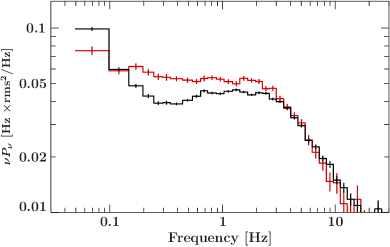
Figure 9: Power spectral densities for the 2004 (A, black) and 2009 (B, red) observations, in the energy range 2.0 – 10.0 keV.

In a scenario where the lags are caused by reflection only at higher frequencies (e.g. with a propagation model explaining the lower-frequency lags) the lags would correspond to reflecting regions close to the central source of direct emission. If this is the case, excluding the lags below a certain frequency would lead to a lower and more plausible $H_{\rm out}/R_{\rm out}$. We therefore exclude lags below 1 Hz from the fit (Table 3) , since this frequency roughly corresponds to the threshold frequency below which the lags relative to softer energies are consistent with being due to propagation of disc fluctuations (Uttley et al., 2011). In addition, this range approximately corresponds to a range in frequency of the PSD (Fig. 9) where the PSD has a similar shape in both observations. Figs 7 and 8 show that when lags at frequencies $<1$ Hz are excluded, the model cannot successfully reproduce either the lag shape or amplitude.

4.1 Consistency of the reflection lags model with optical/UV data

The parameters inferred for the best-fitting reflection model, which are quite extreme and still do not provide a good fit to the lags, can also be checked for the implied effect on optical and UV emission from GX 339–4. X-ray heating of the outer disc could in principle produce a large optical/UV flux if there is a large solid angle illuminated by the continuum, as is the case for the geometry inferred from our lag model fits. We can assume that each illuminated cell in the disc absorbs a fraction of the illuminating continuum equal to $1-a(E)$, so that the incident luminosity absorbed by each cell can be calculated for the best-fitting given continuum shape and model ionisation parameter. If we make the simplifying assumption that the absorbed luminosity dominates over any intrinsic blackbody emission, we can equate the luminosity that is re-emitted by the cell to the absorbed luminosity and so determine the temperature of blackbody radiation emitted by each cell, and hence determine the total reprocessed contribution to the Spectral Energy Distribution (SED).

To compare the predicted contribution to the optical/UV SED from the geometry required by the lags model, we have extracted Swift/UVOT (bands ubb, um2, uuu, uvv, uw1, uw2, uwh) spectra from a 1760 s observation of GX 339–4 made on 29 March 2009, two days after XMM-Newton observed the source. uvot2pha was used to extract spectra for source and background using a 6 arcsec radius, as well as extract response files. No additional aspect correction was required.

From the best-fitting spectral parameters found in fit B’ and assuming a high-energy cut-off at 100 keV (Motta et al., 2011), we derive an X-ray luminosity of $3.5\times 10^{37}$ erg s^-1 (assuming $d=8$ kpc; Zdziarski et al. 2004). This value can be used to predict the reprocessed fluxes that are consistent with the geometries inferred from the fits, accounting for interstellar extinction using the xspec model redden.

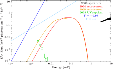
Figure 10: Comparison between expected reprocessed emission using 2009 spectrum with 2004 lags (red) and 2009 lags (orange) and power-law fits to the data with photon indices $-$0.97 (same as low energy tail of reprocessed spectra, in blue) and 1.0 (as expected from synchrotron emission coming from a jet, in light blue) after removing extinction. The data points from UVOT are shown in green.

Fig. 10 shows the expected reprocessed spectra for the two fits to the 2009 X-ray data (orange for B, red for B’, black is the 2009 X-ray spectrum). The photon index $\Gamma$ of the power-law that characterises the reprocessed spectra at the energies covered by the UVOT data is -0.97. In these energy ranges, dust extinction needs to be taken into account using the multiplicative model redden (Cardelli et al., 1989). E(B-V) = 0.933 is the value for the extinction calculated from IR dust maps along the line of sight towards our source. By fitting a power-law with a photon index of -0.97 to the UVOT data, one finds the unabsorbed intrinsic power-law depicted in blue, which has a normalisation in the UVOT energy range that is several decades larger than that expected from reprocessing, and requires E(B-V) = 1.587 for $\chi^{2}$/dof=0.8/4. Therefore the model severely underpredicts the observed flux. A more likely explanation for the optical/UV emission is flat-spectrum synchrotron emission from a compact jet (Maitra et al., 2009), or magnetised hot accretion flow (Veledina et al., 2011). Assuming a power-law photon index of 1.0 (spectral energy index of 0), one also obtains a good fit ($\chi^{2}$/dof=0.64/4) and a lower extinction than in the previous case, E(B-V) = 1.089 (light blue line). This is consistent with the results found by Maitra et al. (2009) for the same object, fitting broadband data using only synchrotron and inverse-Compton models. Therefore, the UVOT data cannot be explained solely by reprocessing in the flared disc envisaged by the lags model and is more likely to be produced by a synchrotron process. However, a small contribution from reprocessing cannot be ruled out.

5 Discussion

5.1 Physical implications

The analysis shown in Section 4 shows that extreme disc geometries are preferred for the model to reproduce the observed lags as closely as possible within the constraints given by the overall spectral shape, including the strength of the iron feature at 6.4 keV. There are several effects of the reprocessing geometry on the spectral and lag data that need to be highlighted to understand why the spectrum can be fitted well, whereas the lags cannot.

Firstly, while the amount of flux in the iron line is proportional to the solid angle subtended by the disc, the ability to determine how much of it is produced in the outer radii of the disc (where Doppler effects are weak) is limited by the resolution of the XMM-Newton EPIC-pn detector. Therefore, the description of the geometry that could be inferred by the spectral modelling alone is degenerate, since line emission from the largest radii (e.g. $\sim 10^{5}$ $R_{\rm g}$) cannot be resolved from that at more modest (but still large) radii (e.g. $\sim 10^{4}$ $R_{\rm g}$). The result of this effect is that the spectral fits are not sensitive to variations in the outer radius of the reflector at large radii.

On the other hand, the lags are very sensitive to the geometry at large radii. Firstly, the lags at low frequencies increase with both the solid angle and light-travel time to the reflector at large radii. A larger outer radius and more flared disc therefore corresponds to larger lags. However, the size-scale of the largest radius also corresponds to a characteristic low-frequency flattening in the lag versus frequency dependence. This is because the frequency-dependent drop in lags seen at higher frequencies is caused by smearing of the reflection variability on time-scales shorter than the light-travel size-scale of the reflector. The reflection variability amplitude is not smeared out for variability time-scales significantly longer than the light-travel time to the largest disc radii, and the lag at low frequencies quickly approaches the average light-travel delay from the reflector (diluted by the direct continuum emission which has zero intrinsic lag). The frequency of this characteristic flattening in the lag-frequency dependence is therefore a sensitive indicator of the size-scale of the reflector. However, it is not possible to reconcile the position of this flattening at frequencies $\sim 0.2$ Hz with the large amplitude of the lags at low frequencies, which imply an even larger reflector subtending an even greater solid angle to the continuum at large radii.

The result of these effects is that despite the already extreme inferred geometries the model is clearly underpredicting the lags. At this point, the maximum value of the lags is now constrained by the spectral modelling, which cannot place a tight constraint on the disc outer radius but does limit the solid angle of the reflector. It is instructive to consider the effects on the predicted spectral shape when the model is fitted to the 2004 lags alone (fixing $\Gamma=1.5$) and the same parameters are used to estimate the resulting spectrum. This yields $\chi^{2}$/dof=66.4/16=4.15 for the fit to the lags and yields an apparent solid angle $\Omega^{\rm eff}/2\pi=1.51$ subtended by the disc. The resulting spectral shape is compared to the data in Fig. 11. Therefore, even fitting the lag data alone with the model cannot produce a good fit, and the fit that is obtained shows that much larger solid angles of large-scale reflection are required than are permitted by the spectrum.

The lags cannot be explained solely by reflection, it is therefore necessary to invoke an additional mechanism to explain them. This result is perhaps not surprising, since we have previously found evidence that in hard state BHXRBs, fluctuations in the accretion disc blackbody emission are correlated with and precede the variations in power-law emission (Uttley et al., 2011). Although the disc variations seem to drive the power-law variations, this does not in itself explain the lags within the power-law band, which we consider in this paper, since the disc emission only extends up to $\sim 2$ keV. However, as we noted in Uttley et al. (2011), at frequencies $<1$ Hz, the lags of the power-law emission relative to the disc-dominated 0.5–0.9 keV band show a similar frequency-dependence to the lags seen within the power-law band (i.e. $\tau\propto\nu^{-0.7}$). This strongly suggests that the lags intrinsic to the power-law are somehow connected to the mechanism which causes the power-law to lag the disc, most probably due to the propagation of accretion fluctuations through the disc before reaching the power-law emitting hot flow.

One possibility is that the disc is sandwiched by the hot-flow/corona which produces power-law emission which becomes harder towards smaller radii, leading to hard lags as fluctuations propagate inwards (e.g. Kotov et al. 2001; Arévalo & Uttley 2006). This model can explain the hard lags in terms of propagation times in the flow, which are much larger than light-crossing times and so can produce relatively large lags which the reflection model struggles to produce without leading to solid angles of large-scale reflection. Reflection may also contribute to the lags at some level, but is not the dominant mechanism, at least at frequencies $<1$ Hz.

A more detailed analysis of the contribution of reflection to the observed lags could be performed using datasets with higher signal-to-noise, by e.g. searching for reflection signatures around the iron line investigated by Kotov et al. (2001). Lags vs. energy spectra for GX 339–4 are shown in Uttley et al. (2011) for the 2004 XMM-Newton observation, and demonstrate that the current quality of the data is not sufficient to detect these features.

It is also possible that multiple distinct components contribute to the lag, e.g. associated with the different Lorentzian features that contribute to the PSD. This possibility could explain the apparent ‘stepping’ of the lag vs. frequency that appears to be linked to the frequencies where the dominant contribution to the PSD changes from one Lorentzian component to another (Nowak, 2000).

5.2 Wider implications of combined spectral-timing models

In this work we have considered (and ruled out) a relatively simple model for the lags in terms of the light-travel times from a large scale reflector. However, it is important to stress the generalisability of our approach to other models. In particular, we have shown how it is possible to combine timing and spectral information to fit models for the geometry and spatial scale of the emitting regions of compact objects. Previous approaches to use the information from time-lags to fit models for the emitting region have focussed on fitting the lag data (e.g. Kotov et al. 2001; Poutanen 2002). However, since these models also make predictions for the spectral behaviour, it is possible to achieve stronger constraints on the models by fitting the lags together with the time-averaged energy spectrum, as done here, or with spectral-variability products such as the frequency-resolved rms and covariance spectra (Revnivtsev et al., 1999; Wilkinson & Uttley, 2009; Uttley et al., 2011).

In order to use these techniques more generally, one needs to calculate the energy-dependent response function for the emitting region, i.e. determine the emission as a function of time delay and energy. This approach can be used to test reverberation models for the small soft lags seen at high frequencies in AGN (Fabian et al., 2009; Zoghbi et al., 2010; de Marco et al., 2011; Emmanoulopoulos et al., 2011) and BHXRBs (Uttley et al., 2011), which offers the potential to map the emitting region on scales within a few gravitational radii of the black hole. Other models can also be considered, e.g. to test the propagation models for the low-frequency lags with the time-delay expressed in terms of propagation time through the accretion flow. Future, large-area X-ray detectors with high time and energy-resolution, such as the proposed ATHENA and LOFT missions, will allow much more precise measurements of the lags in combination with good spectral measurements, so that fitting of combined models for spectral and timing data could become a default approach for studying the innermost regions of compact objects. Future research in this direction is strongly encouraged.

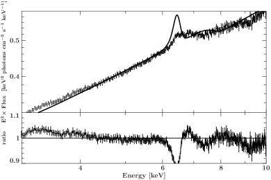
Figure 11: Spectral model (reflags) compared to 2004 spectrum using the parameters that are derived from fitting the 2004 lags alone. The lower panel shows the ratio data/model.

References

- Arévalo & Uttley (2006) Arévalo P., Uttley P., 2006, MNRAS, 367, 801
- Ballantyne et al. (2001) Ballantyne D. R., Iwasawa K., Fabian A. C., 2001, MNRAS, 323, 506
- Bendat & Piersol (2010) Bendat, J. S., Piersol, A. G., 2010, Random data: Analysis and measurement procedures. Wiley, New York
- Cardelli et al. (1989) Cardelli J. A., Clayton G. C., Mathis J. S., 1989, IAUS, 135, 5P
- de Marco et al. (2011) de Marco B., Ponti G., Uttley P., Cappi M., Dadina M., Fabian A. C., Miniutti G., 2011, MNRAS, 417, L98
- Cui et al. (1997) Cui W., Zhang S. N., Focke W., Swank J. H., 1997, ApJ, 484, 383
- Done & Diaz Trigo (2010) Done C., Diaz Trigo M., 2010, MNRAS, 407, 2287
- Emmanoulopoulos et al. (2011) Emmanoulopoulos D., McHardy I. M., Papadakis I. E., 2011, MNRAS, 416, L94
- Fabian et al. (1989) Fabian A. C., Rees M. J., Stella L., White N. E., 1989, MNRAS, 238, 729
- Fabian et al. (2009) Fabian A. C., et al., 2009, Nat, 459, 540
- Fabian & Ross (2010) Fabian A. C., Ross R. R., 2010, SSRv, 157, 167
- George & Fabian (1991) George I. M., Fabian A. C., 1991, MNRAS, 249, 352
- Kazanas et al. (1997) Kazanas D., Hua X.-M., Titarchuk L., 1997, ApJ, 480, 735
- Kotov et al. (2001) Kotov O., Churazov E., Gilfanov M., 2001, MNRAS, 327, 799
- Kuster et al. (2002) Kuster M., Kendziorra E., Benlloch S., Becker W., Lammers U., Vacanti G., Serpell E., 2002, arXiv:astro-ph/0203207
- Kylafis et al. (2008) Kylafis N. D., Papadakis I. E., Reig P., Giannios D., Pooley G. G., 2008, A&A, 489, 481
- Lyubarskii (1997) Lyubarskii Y. E., 1997, MNRAS, 292, 679
- Maccarone et al. (2000) Maccarone T. J., Coppi P. S., Poutanen J., 2000, ApJ, 537, L107
- Maitra et al. (2009) Maitra D., Markoff S., Brocksopp C., Noble M., Nowak M., Wilms J., 2009, MNRAS, 398, 1638
- Miyamoto et al. (1988) Miyamoto S., Kitamoto S., Mitsuda K., Dotani T., 1988, Nat, 336, 450
- Motta et al. (2011) Motta S., Belloni T., Homan J., 2009, MNRAS, 400, 1603
- Nowak et al. (1999) Nowak M. A., Vaughan B. A., Wilms J., Dove J. B., Begelman M. C., 1999, ApJ, 510, 874
- Nowak (2000) Nowak M. A., 2000, MNRAS, 318, 361
- Poutanen (2001) Poutanen J., 2001, Adv. Sp. Res., 28, 267
- Poutanen (2002) Poutanen J., 2002, MNRAS, 332, 257
- Poutanen & Fabian (1999) Poutanen J., Fabian A. C., 1999, MNRAS, 306, L31
- Reig et al. (2003) Reig P., Kylafis N. D., Giannios D., 2003, A&A, 403, L15
- Revnivtsev et al. (1999) Revnivtsev M., Gilfanov M., Churazov E., 1999, A&A, 347, L23
- Tomsick et al. (2009) Tomsick J. A., Yamaoka K., Corbel S., Kaaret P., Kalemci E., Migliari S., 2009, ApJ, 707, L87
- Uttley & McHardy (2001) Uttley P., McHardy I. M., 2001, MNRAS, 323, L26
- Uttley et al. (2011) Uttley P., Wilkinson T., Cassatella P., Wilms J., Pottschmidt K., Hanke M., Böck M., 2011, MNRAS, 414, L60
- Veledina et al. (2011) Veledina A., Poutanen J., Vurm I., 2011, ApJ, 737, L17
- Wilkinson (2011) Wilkinson T., 2011, PhD thesis, University of Southampton
- Wilkinson & Uttley (2009) Wilkinson T., Uttley P., 2009, MNRAS, 397, 666
- Zdziarski et al. (2004) Zdziarski A. A., Gierliński M., Mikołajewska J., Wardziński G., Smith D. M., Harmon B. A., Kitamoto S., 2004, MNRAS, 351, 791
- Zoghbi et al. (2010) Zoghbi A., Fabian A. C., Uttley P., Miniutti G., Gallo L. C., Reynolds C. S., Miller J. M., Ponti G., 2010, MNRAS, 401, 2419